Data-Driven Spectrum Cartography via
Deep Completion AutoencodersThanks: Emails: {yves.teganya, daniel.romero}@uia.no. This work was supported by the Research Council of Norway through the FRIPRO TOPPFORSK grant 250910/F20 and the INDNOR program under the LUCAT project. The authors thank Prof. Baltasar Beferull-Lozano for funding and administrative support.

Yves Teganya Affiliation: Dept. of Information and Communication Technology, University of Agder, Norway. Affiliation: Intelligent Signal Processing and Wireless Networks Laboratory (WISENET) Daniel Romero Affiliation: Dept. of Information and Communication Technology, University of Agder, Norway.

Abstract

Spectrum maps, which provide RF spectrum metrics such as power spectral density for every location in a geographic area, find numerous applications in wireless communications such as interference control, spectrum management, resource allocation, and network planning to name a few. Spectrum cartography techniques construct these maps from a collection of measurements collected by spatially distributed sensors. Due to the nature of the propagation of electromagnetic waves, spectrum maps are complicated functions of the spatial coordinates. For this reason, model-free approaches have been preferred. However, all existing schemes rely on some interpolation algorithm unable to learn from data. This work proposes a novel approach to spectrum cartography where propagation phenomena are learned from data. The resulting algorithms can therefore construct a spectrum map from a significantly smaller number of measurements than existing schemes since the spatial structure of shadowing and other phenomena is previously learned from maps in other environments. Besides the aforementioned new paradigm, this is also the first work to perform spectrum cartography with deep neural networks. To exploit the manifold structure of spectrum maps, a deep network architecture is proposed based on completion autoencoders.

I Introduction

Spectrum cartography constructs maps of RF channel metrics such as received signal power, interference power, power spectral density (PSD), electromagnetic absorption, or channel gain; see e.g. [1, 2, 3]. Besides applications like source localization [2] or radio tomography [4, 5], spectral maps find a myriad of applications in wireless communications such as network planning, interference coordination, power control, spectrum management, resource allocation, handoff procedure design, dynamic spectrum access, and cognitive ratio [6, 7, 8]. Spectrum maps are constructed from measurements acquired by spectrum sensors or mobile devices.

Most approaches are based on some interpolation algorithm. For example, power maps have been constructed through kriging [1, 9], dictionary learning [10, 11], compressive sensing [3], Bayesian models [12], matrix completion [13], and kernel methods [14, 15]. PSD maps have also been constructed by exploiting the sparsity of power across space and frequency [2] as well as by applying thin-plate spline regression [16] and kernel-based learning [8, 17]. Metrics other than power and PSD have also been mapped in the literature. For example, [18, 5, 19] are capable of constructing channel gain maps. Unfortunately, none of the existing approaches can learn from data. This means that they fail to learn the characteristics of the propagation phenomena and, therefore, a substantial performance improvement is expected if such knowledge can be incorporated.

To address this limitation, the first contribution of this work is a data-driven paradigm for spectrum cartography. Specifically, it proposes learning the spatial features of the relevant propagation phenomena such as shadowing, reflection, and diffraction using a data set of past measurements. Intuitively, leveraging these learned features can significantly reduce the number of measurements required to attain a target performance. This aspect is critical since all measurements need to be collected in a sufficiently short time since the mapped metric is subject to temporal variations in real-world scenarios. The second contribution comprises a spectrum cartography algorithm to construct PSD maps relying on a deep neural network. Although several approaches for applying this class of networks are discussed, the most natural one relies on a spatial discretization of the area of interest. The resulting tensor completion task is addressed by means of a completion network architecture with an encoder-decoder structure that capitalizes on the observation that spectrum maps lie close to a low-dimensional manifold embedded in a high-dimensional space. Our experiments reveal that the performance of such algorithm beats the state-of-the-art alternatives. Finally, all code, trained networks, and the data set constructed for this work will be posted at the authors’ web sites.

The novelty of this work is twofold. First, this is the first work to propose a data-driven spectrum cartography approach. Second, this is the first work to propose a deep learning algorithm for spectrum cartography.

The rest of this report is organized as follows. Sec. II describes the problem of PSD cartography. Sec. III presents the aforementioned data-driven spectrum cartography paradigm and proposes a deep neural network architecture based on completion autoencoders. Simulations and conclusions are respectively provided in Secs. IV and V.

Notation: $|\mathcal{A}|$ denotes the cardinality of set $\mathcal{A}$ . $[\bm{A}]_{i,j}$ is the $(i,j)$ -th entry of matrix $\bm{A}$ , whereas $[\bm{B}]_{i,j,k}$ is the $(i,j,k)$ -th entry of tensor $\bm{B}$ . Finally, $\bm{A}^{\top}$ is the transpose of matrix $\bm{A}$ .

II Model and Problem Formulation

Consider ${{\color[rgb]{0,0,0}S}}$ sources located in a geographical region of interest $\mathcal{X}\subset\mathbb{R}^{2}$ and operating on a certain frequency band. Let ${{\color[rgb]{0,0,0}\Upsilon}}_{{{\color[rgb]{0,0,0}s}}}(f)$ denote the transmit PSD of the ${{\color[rgb]{0,0,0}s}}$ -th source and let $H_{{{\color[rgb]{0,0,0}s}}}(\bm{x},f)$ represent the frequency response of the channel between the ${{\color[rgb]{0,0,0}s}}$ -th source and a sensor with an isotropic antenna located at $\bm{x}\in\mathcal{X}$ . For simplicity, assume that small-scale fading has been averaged out; see also Remark 1. Both ${{\color[rgb]{0,0,0}\Upsilon}}_{{{\color[rgb]{0,0,0}s}}}(f)$ and $H_{{{\color[rgb]{0,0,0}s}}}(\bm{x},f)$ are assumed to remain constant over time, a realistic assumption provided that the measurements described below are collected in an interval of shorter length than the channel coherence time and time scale of changes in ${{\color[rgb]{0,0,0}\Upsilon}}_{{{\color[rgb]{0,0,0}s}}}(f)$ .

If the ${{\color[rgb]{0,0,0}S}}$ signals are uncorrelated, the PSD at $\bm{x}\in\mathcal{X}$ is ${{\color[rgb]{0,0,0}\Psi}}(\bm{x},f)=\textstyle\sum_{{{\color[rgb]{0,0,0}s}}=1}^{{{\color[rgb]{0,0,0}S}}}{{\color[rgb]{0,0,0}\Upsilon}}_{{{\color[rgb]{0,0,0}s}}}(f)|H_{{{\color[rgb]{0,0,0}s}}}(\bm{x},f)|^{2}+\upsilon(\bm{x},f)$ with $\upsilon(\bm{x},f)$ the noise PSD of a generic sensor at location $\bm{x}$ , which models thermal noise, background radiation noise, and interference from remote sources. A certain number of devices, such as mobile users in a cellular communication network or spectrum sensors, collect PSD measurements $\{\tilde{{\color[rgb]{0,0,0}\Psi}}(\bm{x}_{n},f)\}_{n=1}^{N}$ at $N$ locations $\{\bm{x}_{n}\}_{n=1}^{N}\subset\mathcal{X}$ and finite set of frequencies $f\in\mathcal{F}$ ; see also Remark 2. These measurements can be obtained using e.g. periodograms or spectral analysis methods such as the Bartlett or Welch method [20].

These measurements are sent to a fusion center, which may be e.g. a base station, a mobile user, or a cloud server, depending on the application. Given $\{(\bm{x}_{n},\tilde{{\color[rgb]{0,0,0}\Psi}}(\bm{x}_{n},f)),~n=1,\ldots,N,~f\in\mathcal{F}\}$ , the fusion center must obtain an estimate $\hat{{{\color[rgb]{0,0,0}\Psi}}}(\bm{x},f)$ of ${{\color[rgb]{0,0,0}\Psi}}(\bm{x},f)$ at every location $\bm{x}\in\mathcal{X}$ and frequency $f\in\mathcal{F}$ . In spectrum cartography, function ${{\color[rgb]{0,0,0}\Psi}}(\bm{x},f)$ is typically referred to as the true map, whereas $\hat{{{\color[rgb]{0,0,0}\Psi}}}(\bm{x},f)$ is the estimated map or map estimate. The algorithm or rule that provides a map estimate, which in this work is a neural network, is termed map estimator. The challenge is to exploit the spatial structure of propagation phenomena so that the estimation error, quantified e.g. as $\sum_{f}\int_{\mathcal{X}}|{{\color[rgb]{0,0,0}\Psi}}(\bm{x},f)-\hat{{\color[rgb]{0,0,0}\Psi}}(\bm{x},f)|^{2}d\bm{x}$ , is minimized for a certain $N$ or, alternatively, the minimum $N$ required to guarantee a target estimation error is minimized.

To the best of our knowledge, all existing approaches to spectrum cartography are based on interpolation algorithms that do not learn from data. In contrast, the next section develops a novel data-driven methodology that learns the aforementioned structure from a data set.

Remark 1

Sensors must determine their locations $\{\bm{x}_{n}\}_{n}$ with an error sufficiently small relative to the scale of spatial variability of ${\color[rgb]{0,0,0}\Psi}(\bm{x},f)$ across $\mathcal{X}$ . Thus, estimating small-scale fading is more challenging than estimating shadowing since the coherence distance of the former is comparable to the wavelength and typical communication bands of interest have wavelengths in the order of centimeters.

Remark 2

The number of measurement locations may be significantly larger than the number of sensors if the sensors move. Measurements collected at different locations may be useful to estimate a spectrum map so long as the difference between measurement instants is small relative to the time scale of the variations of the PSD map. The latter is highly dependent on the specific application. For example, one expects significant variations in DVB-T bands to occur in the scale of several months, whereas PSD maps in LTE bands may change in the scale of milliseconds due to power control, mobility, and interference.

III Proposed Data-Driven Cartography

This section introduces a data-driven paradigm for spectrum cartography and develops a deep learning algorithm that abides by this principle. To this end, Sec. III-A starts by reformulating the problem at hand as a tensor-completion task amenable to application of deep neural networks. Subsequently, Sec. III-B addresses unique aspects of tensor/matrix completion via deep learning. Finally, Secs. III-C and III-D respectively describe how a deep neural network can be trained to learn the spatial structure of propagation phenomena and how this task can be addressed via the notion of completion autoencoders.

III-A Spectrum Cartography as a Tensor Completion Task

Observe that the value of $N$ depends on the number and movement of the sensors relative to the time-scale of temporal changes in ${{\color[rgb]{0,0,0}\Psi}}(\bm{x},f)$ ; cf. Sec. II. In principle, one could think of using a separate map estimator for each possible value of $N$ . Each estimator could be relatively simple since it would always take the same number of inputs. However, such an approach would be highly inefficient in terms of memory, computation, and prone to erratic behavior since each estimator is trained with a different data set. Thus, it is more practical to rely on a single estimator that can accommodate arbitrary values of $N$ . A customary approach in deep learning for coping with inputs of variable lengths is through recurrent neural networks [21],[22, Ch. 10]. Unfortunately, besides the difficulties of training these networks, it is unclear how such an approach could effectively exploit spatial information. For this reason, the selected approach in this work is to reformulate the cartography problem as a tensor completion task amenable to a solution based on a feedforward architecture [22, Ch. 6].

Refer to caption — Fig. 1: Model setup and area discretization.

To this end, one must discretize $\mathcal{X}$ , a trick already applied in radio tomographic imaging [23, 24] and spectrum cartography [13]. To introduce the appropriate notation, it will be briefly outlined next. Define an $N_{y}\times N_{x}$ rectangular grid over $\mathcal{X}$ , as depicted in Fig. 1. This grid comprises points ${{\color[rgb]{0,0,0}\bm{\xi}}}_{i,j}$ evenly spaced by $\Delta_{x}$ and $\Delta_{y}$ along the $x$ - and $y$ -axes respectively, that is, the $(i,j)$ -th grid point is given by ${{\color[rgb]{0,0,0}\bm{\xi}}}_{i,j}:=\left[i\Delta_{x},~j\Delta_{y}\right]^{\top}$ , with $~i=1,\ldots,N_{y},~j=1,\ldots,N_{x}$ . For future usage, define $\mathcal{A}_{i,j}\subset\{1,\ldots,N\}$ as the set containing the indices of the measurement locations assigned to the $(i,j)$ -th grid point by the criterion of minimum distance, i.e., $n\in\mathcal{A}_{i,j}$ iff $||{{\color[rgb]{0,0,0}\bm{\xi}}}_{i,j}-\bm{x}_{n}||\leq||{{\color[rgb]{0,0,0}\bm{\xi}}}_{i^{\prime},j^{\prime}}-\bm{x}_{n}||\forall i^{\prime},j^{\prime}$ with $i^{\prime}\neq i$ and $j^{\prime}\neq j$ .

This grid induces a discretization of ${\color[rgb]{0,0,0}\Psi}(\bm{x},f)$ along the $\bm{x}$ variable. One can therefore collect the true PSD values at the grid points in matrix $\bm{{\color[rgb]{0,0,0}\Psi}}(f)\in\mathbb{R}^{N_{y}\times N_{x}}$ , $f\in\mathcal{F}$ , whose $(i,j)$ -th entry is given by $\left[\bm{{\color[rgb]{0,0,0}\Psi}}(f)\right]_{i,j}={{\color[rgb]{0,0,0}\Psi}}({{\color[rgb]{0,0,0}\bm{\xi}}}_{i,j},f)$ . By letting $\mathcal{F}=\{f_{1},\ldots,f_{N_{f}}\}$ , it is also possible to stack these matrices along the third dimension to form the tensor $\bm{{\color[rgb]{0,0,0}\Psi}}\in\mathbb{R}^{N_{y}\times N_{x}\times N_{f}}$ , where $\left[\bm{{\color[rgb]{0,0,0}\Psi}}\right]_{i,j,n_{f}}={{\color[rgb]{0,0,0}\Psi}}({{\color[rgb]{0,0,0}\bm{\xi}}}_{i,j},f_{n_{f}})$ , $n_{f}=1,\ldots,N_{f}$ . For short, the term true map will either refer to ${{\color[rgb]{0,0,0}\Psi}}(\bm{x},f)$ or $\bm{{\color[rgb]{0,0,0}\Psi}}$ .

Similarly, one can collect the measurements in a tensor of the same dimensions. Informally, if the grid is sufficiently fine ( $\Delta_{x}$ and $\Delta_{y}$ are sufficiently small), it holds that $\bm{x}_{n}\approx{{\color[rgb]{0,0,0}\bm{\xi}}}_{i,j}$ $\forall n\in\mathcal{A}_{i,j}$ and, correspondingly, ${{\color[rgb]{0,0,0}\Psi}}(\bm{x}_{n},f)\approx{{\color[rgb]{0,0,0}\Psi}}({{\color[rgb]{0,0,0}\bm{\xi}}}_{i,j},f)$ $\forall n\in\mathcal{A}_{i,j}$ . It follows that, ${{\color[rgb]{0,0,0}\Psi}}({{\color[rgb]{0,0,0}\bm{\xi}}}_{i,j},f)\approx({1}/{|\mathcal{A}_{i,j}|)}\sum_{n\in\mathcal{A}_{i,j}}{{\color[rgb]{0,0,0}\Psi}}(\bm{x}_{n},f)$ whenever $|\mathcal{A}_{i,j}|\geq 1$ . Therefore, it makes sense to aggregate all the measurements assigned to ${{\color[rgb]{0,0,0}\bm{\xi}}}_{i,j}$ as¹¹ 1 For simplicity, the notation implicitly assumes that $\bm{x}_{n}\neq{{\color[rgb]{0,0,0}\bm{\xi}}}_{i,j}$ $\forall n,i,j$ , but this is not a requirement. $\tilde{{\color[rgb]{0,0,0}\Psi}}({{\color[rgb]{0,0,0}\bm{\xi}}}_{i,j},f){:=}({1}/{|\mathcal{A}_{i,j}|})\sum_{n\in\mathcal{A}_{i,j}}\tilde{{\color[rgb]{0,0,0}\Psi}}(\bm{x}_{n},f).$ Conversely, when $|\mathcal{A}_{i,j}|=0$ , there are no measurements associated with ${{\color[rgb]{0,0,0}\bm{\xi}}}_{i,j}$ , in which case one says that there is a miss at ${{\color[rgb]{0,0,0}\bm{\xi}}}_{i,j}$ . Upon letting $\Omega\subset\{1,\ldots,N_{y}\}\times\{1,\ldots,N_{x}\}$ be such that $(i,j)\in\Omega$ iff $|\mathcal{A}_{i,j}|>0$ , all (possibly aggregated) measurements $\tilde{{\color[rgb]{0,0,0}\Psi}}({{\color[rgb]{0,0,0}\bm{\xi}}}_{i,j},f)$ can be collected in $\tilde{\bm{{\color[rgb]{0,0,0}\Psi}}}(f)\in\mathbb{R}^{N_{y}\times N_{x}}$ , defined as $[\tilde{\bm{{\color[rgb]{0,0,0}\Psi}}}(f)]_{i,j}=\tilde{{\color[rgb]{0,0,0}\Psi}}({{\color[rgb]{0,0,0}\bm{\xi}}}_{i,j},f)$ if $(i,j)\in\Omega$ and $[\tilde{\bm{{\color[rgb]{0,0,0}\Psi}}}(f)]_{i,j}=0$ otherwise. Note that misses have been filled with zeroes, but other values can be used.

When $(i,j)\in\Omega$ , the values of $[\tilde{\bm{{\color[rgb]{0,0,0}\Psi}}}(f)]_{i,j}$ and $[{\bm{{\color[rgb]{0,0,0}\Psi}}}(f)]_{i,j}$ differ due to the error introduced by the spatial discretization as well as due to the measurement error incurred when measuring ${\color[rgb]{0,0,0}\Psi}(\bm{x}_{n},f),~n\in\mathcal{A}_{i,j}$ . The latter is caused mainly by the finite time devoted by sensors to take measurements.

As before, the matrices ${\tilde{\bm{{\color[rgb]{0,0,0}\Psi}}}}(f),~f=1,\ldots,N_{f}$ can be stacked along the 3rd dimension to form ${\tilde{\bm{{\color[rgb]{0,0,0}\Psi}}}}\in\mathbb{R}^{N_{y}\times N_{x}\times N_{f}}$ , where $[{\tilde{\bm{{\color[rgb]{0,0,0}\Psi}}}}]_{i,j,n_{f}}=[{\tilde{\bm{{\color[rgb]{0,0,0}\Psi}}}}(f_{n_{f}})]_{i,j}$ . For short, this tensor will be referred to as the sampled map.

The cartography problem stated in Sec. II can now be reformulated as, given $\Omega$ and ${\tilde{\bm{{\color[rgb]{0,0,0}\Psi}}}}$ , estimate $\bm{{\color[rgb]{0,0,0}\Psi}}$ .

III-B Feedforward Completion Networks

The previous section reformulated the spectrum cartography problem as a tensor completion task. Since conventional neural networks cannot directly accommodate input misses and set-valued inputs like $\Omega$ , this section explores the possibilities and motivates the adopted approach.

But before that, a quick refresh on deep learning is in order. A feedforward deep neural network is a function ${\color[rgb]{0,0,0}p_{\bm{w}}}$ that can be expressed as the composition ${\color[rgb]{0,0,0}p_{\bm{w}}}({{\color[rgb]{0,0,0}\bm{\Phi}}})={\color[rgb]{0,0,0}p}^{{\color[rgb]{0,0,0}(}{\color[rgb]{0,0,0}L}{\color[rgb]{0,0,0})}}_{\bm{w}_{{\color[rgb]{0,0,0}L}}}({\color[rgb]{0,0,0}p}^{{\color[rgb]{0,0,0}(}{\color[rgb]{0,0,0}L}-1{\color[rgb]{0,0,0})}}_{\bm{w}_{{\color[rgb]{0,0,0}L}-1}}(\ldots{\color[rgb]{0,0,0}p}^{{\color[rgb]{0,0,0}(}1{\color[rgb]{0,0,0})}}_{\bm{w}_{1}}({{\color[rgb]{0,0,0}\bm{\Phi}}})))$ of layer functions ${\color[rgb]{0,0,0}p}^{{\color[rgb]{0,0,0}(}{{\color[rgb]{0,0,0}l}}{\color[rgb]{0,0,0})}}_{\bm{w}_{{\color[rgb]{0,0,0}l}}}$ , where ${{\color[rgb]{0,0,0}\bm{\Phi}}}$ is the input. Although there is no commonly agreed definition of layer function, it is typically formed by concatenating simple scalar-valued functions termed neurons that implement a linear function followed by a simple non-linear function known as activation [22]. The term neuron stems from the resemblance between these functions and certain simple functional models for natural neurons. Similarly, there is no consensus on which values of ${\color[rgb]{0,0,0}L}$ qualify for ${\color[rgb]{0,0,0}p_{\bm{w}}}$ to be considered a deep neural network. With vector $\bm{w}_{{\color[rgb]{0,0,0}l}}$ containing the parameters of the ${{\color[rgb]{0,0,0}l}}$ -th layer, the parameters of the entire network can be collected in $\bm{w}{:=}[\bm{w}_{1}^{\top},\ldots,\bm{w}_{{\color[rgb]{0,0,0}L}}^{\top}]^{\top}\in\mathbb{R}^{N_{w}}$ . These parameters are learned using a training set in a process termed training.

The rest of this section as well as Sec. III-C carefully delineate how a deep neural network can be trained to perform data-driven spectrum cartography. Occasional references to works in areas such as collaborative filtering and image inpainting will provide insight and motivate the design decisions. On the other hand, Sec. III-D will address the design of ${\color[rgb]{0,0,0}p_{\bm{w}}}$ .

Although the training set construction is detailed in Sec. III-C, suppose by now that a set of $T$ training examples $\{({\tilde{\bm{{\color[rgb]{0,0,0}\Psi}}}}_{t},\Omega_{t})\}_{t=1}^{T}$ is given. Here, $\{{\tilde{\bm{{\color[rgb]{0,0,0}\Psi}}}}_{t}\}_{t}$ is a collection of sampled maps acquired in different environments and $\Omega_{t}$ the corresponding sampling set.

The desired estimator should obtain $\bm{{\color[rgb]{0,0,0}\Psi}}$ as a function of ${\tilde{\bm{{\color[rgb]{0,0,0}\Psi}}}}$ and $\Omega$ . But regular neural networks cannot directly accommodate set-valued inputs and missing entries. For this reason, [25] proposes filling the missing entries in ${\tilde{\bm{{\color[rgb]{0,0,0}\Psi}}}}$ by solving

	$\displaystyle\underset{\{{\color[rgb]{0,0,0}\bm{\chi}}_{t}\}_{t},\bm{w}}{\text{minimize}}\quad$	$\displaystyle\frac{1}{T}\sum_{t=1}^{T}\left\\|\mathcal{P}_{\Omega_{t}}\left({\color[rgb]{0,0,0}\bm{\chi}}_{t}-p_{\bm{w}}({\color[rgb]{0,0,0}\bm{\chi}}_{t})\right)\right\\|_{F}^{2},$		(1)
	$\displaystyle\mathop{\text{s.t.}}\quad$	$\displaystyle[{\color[rgb]{0,0,0}\bm{\chi}}_{t}]_{i,j,n_{f}}=[{\tilde{\bm{{\color[rgb]{0,0,0}\Psi}}}}_{t}]_{i,j,n_{f}}~\forall n_{f},\forall(i,j)\in\Omega_{t},$

where $||\bm{A}||_{F}^{2}{:=}\sum_{i,j,n_{f}}[\bm{A}]_{i,j,n_{f}}^{2}$ is the Frobenius norm of tensor $\bm{A}$ and $\mathcal{P}_{\Omega}(\bm{A})$ is defined as $\left[\mathcal{P}_{\Omega}(\bm{A})\right]_{i,j,n_{f}}=[\bm{A}]_{i,j,n_{f}}$ if $(i,j)\in\Omega$ and $\left[\mathcal{P}_{\Omega}(\bm{A})\right]_{i,j,n_{f}}=0$ otherwise. The map estimate produced by this method is directly the minimizer ${\color[rgb]{0,0,0}\bm{\chi}}_{t}$ of (1). Observe that if there exists a value of $\bm{w}$ for which ${\color[rgb]{0,0,0}p_{\bm{w}}}$ becomes the identity map, i.e. ${\color[rgb]{0,0,0}\bm{\chi}}=p_{\bm{w}}({\color[rgb]{0,0,0}\bm{\chi}}),~\forall{\color[rgb]{0,0,0}\bm{\chi}}$ , then the optimum of (1) is attained regardless of the value of the entries $[{\color[rgb]{0,0,0}\bm{\chi}}_{t}]_{i,j,n_{f}},~(i,j)\notin\Omega_{t}$ , which would render this estimator useless. Thus, some form of capacity/complexity control is necessary [26]. For instance, one can (i) impose constraints on $\bm{w}$ , (ii) add a regularization term to the objective function, or (iii) limit capacity through the design of the network architecture. Approach (iii) will be discussed further in Sec. III-D. To simplify the exposition, expressions in this report will not display constraints or regularizers, but it is understood that the user may include them if necessary.

After $\bm{w}={\hat{\bm{w}}}$ has been obtained by applying (1) with sufficiently large $T$ , one can complete further tensors ${\tilde{\bm{{\color[rgb]{0,0,0}\Psi}}}}_{t}$ by setting $\bm{w}$ in (1) to this learned vector ${\hat{\bm{w}}}$ and optimize only with respect to $\{{\color[rgb]{0,0,0}\bm{\chi}}_{t}\}_{t}$ , which is computationally simpler.

The number of optimization variables in (1) is $N_{w}+N_{x}N_{y}N_{f}T$ , where $N_{w}$ is the length of $\bm{w}$ . This number is prohibitive for high $T$ , as required for training deep neural networks. Besides, even with the aforementioned simplified approach that only optimizes with respect to $\{{\color[rgb]{0,0,0}\bm{\chi}}_{t}\}_{t}$ , a large number of forward and backward backpropagation passes [22, Ch. 6] are required to estimate each map. Thus, this approach is not suitable for real-time implementation, as required in spectrum cartography applications.

To alleviate this limitation, a simple alternative would be to just feed ${\tilde{\bm{{\color[rgb]{0,0,0}\Psi}}}}$ to the neural network and train by solving

\displaystyle\underset{\bm{w}}{\text{minimize}}\quad

\displaystyle\textstyle\frac{1}{T}\sum_{t=1}^{T}\left\|\mathcal{P}_{\Omega_{t}}\left({\tilde{\bm{{\color[rgb]{0,0,0}\Psi}}}}_{t}-p_{\bm{w}}({\tilde{\bm{{\color[rgb]{0,0,0}\Psi}}}}_{t})\right)\right\|_{F}^{2}.

(2)

Although the missing entries were filled with zeros in Sec. III-A, one can alternatively use other real numbers. After (2) is solved, ${\tilde{\bm{{\color[rgb]{0,0,0}\Psi}}}}$ can be completed just by evaluating $p_{\bm{w}}({\tilde{\bm{{\color[rgb]{0,0,0}\Psi}}}})$ , which requires a single forward pass. Besides, solving (2) involves just $N_{w}$ optimization variables. However, because the completion step $p_{\bm{w}}({\tilde{\bm{{\color[rgb]{0,0,0}\Psi}}}})$ does not involve $\Omega$ , poor performance is expected since the network cannot distinguish missing entries from measurements close to the filling value.

In the application at hand, one could circumvent this limitation by expressing the entries of ${\tilde{\bm{{\color[rgb]{0,0,0}\Psi}}}}$ in natural power units (e.g. Watt) and filling the misses with a negative number such as -1. Unfortunately, the usage of finite-precision arithmetic would introduce large errors in the map estimates and is problematic in our experience. For this reason, expressing ${\tilde{\bm{{\color[rgb]{0,0,0}\Psi}}}}$ in logarithmic units such as dBm is preferable. However, the problem of distinguishing missing entries persists since logarithmic units are not confined to be non-negative.

A more practical approach is to complement the input of the network with a binary mask that indicates which entries are observed, as proposed in the image inpainting literature [27]. In this case, the binary mask $\bm{{\color[rgb]{0,0,0}M}}_{\Omega}\in\{0,1\}^{N_{y}\times N_{x}}$ associated with the sampling set $\Omega$ is given by $[\bm{{\color[rgb]{0,0,0}M}}_{\Omega}]_{i,j}=1$ if $(i,j)\in\Omega$ and $[\bm{{\color[rgb]{0,0,0}M}}_{\Omega}]_{i,j}=0$ otherwise.

To simplify notation, let ${{\check{\bm{{\color[rgb]{0,0,0}\Psi}}}}}\in\mathbb{R}^{N_{y}\times N_{x}\times N_{f}+1}$ denote a tensor obtained by concatenating ${\tilde{\bm{{\color[rgb]{0,0,0}\Psi}}}}$ and $\bm{{\color[rgb]{0,0,0}M}}_{\Omega}$ along the third dimension. The neural network can therefore be trained as

\displaystyle\underset{\bm{w}}{\text{minimize}}\quad

\displaystyle\textstyle\frac{1}{T}\sum_{t=1}^{T}\left\|\mathcal{P}_{\Omega_{t}}\left({\tilde{\bm{{\color[rgb]{0,0,0}\Psi}}}}_{t}-p_{\bm{w}}({{\check{\bm{{\color[rgb]{0,0,0}\Psi}}}}}_{t})\right)\right\|_{F}^{2}

(3)

and, afterwards, a tensor ${\tilde{\bm{{\color[rgb]{0,0,0}\Psi}}}}$ can be completed just by evaluating $p_{\bm{w}}({{\check{\bm{{\color[rgb]{0,0,0}\Psi}}}}})$ . Then, this scheme is simple to train, inexpensive to test, and exploits information about the location of the misses.

III-C Learning in Real-World Scenarios

A key novelty in this work is to obtain map estimators by learning from data. This section describes how to construct a suitable training set in the application at hand.

The first consideration pertains to ill-conditioning issues arising when the number of frequencies $N_{f}$ in $\mathcal{F}$ is large, as will typically be the case. Suppose that the first layer of ${\color[rgb]{0,0,0}p_{\bm{w}}}$ is fully connected and has $N_{N}$ neurons. Its total number of parameters becomes $(N_{y}N_{x}N_{f}+1)N_{N}$ plus possibly additional parameters of the activation functions. Other layers will experience the same issue to different extents. Since $T$ must be comparable to the number of unknowns to train the network effectively, the impact of a large $N_{f}$ is to drastically limit the number of layers or neurons that can be used.

Previous approaches in spectrum cartography experienced similar issues, which were often addressed by the introduction of parametric models along the frequency domain; see e.g. [16, 8]. Although such an approach can be similarly adopted in the present work, thereby reducing the number of channels at the neural network input from $N_{f}+1$ to a much smaller number, it will be argued next that directly separating the problem across frequencies may be preferable when training a deep neural network. The idea is that propagation phenomena at similar frequencies are expected to be similar. Building upon this principle, ${\color[rgb]{0,0,0}p_{\bm{w}}}$ can operate separately at each frequency $f$ . This means that training can be accomplished through

\displaystyle\underset{\bm{w}}{\text{min.}}~

\displaystyle\frac{1}{TN_{f}}\sum_{t=1}^{T}\sum_{f\in\mathcal{F}}\left\|\mathcal{P}_{\Omega_{t}}\left({\tilde{\bm{{\color[rgb]{0,0,0}\Psi}}}}_{t}(f)-p_{\bm{w}}({{\check{\bm{{\color[rgb]{0,0,0}\Psi}}}}}_{t}(f))\right)\right\|_{F}^{2},

(4)

where ${{\check{\bm{{\color[rgb]{0,0,0}\Psi}}}}}_{t}(f)\in\mathbb{R}^{N_{y}\times N_{x}\times 2}$ is a tensor with first frontal slab given by ${\tilde{\bm{{\color[rgb]{0,0,0}\Psi}}}}_{t}(f)$ and second frontal slab given by $\bm{{\color[rgb]{0,0,0}M}}_{\Omega_{t}}$ .

Observe that the number of variables is now reduced by a factor of $N_{f}$ whereas the “effective” number of training examples has been multiplied by $N_{f}$ ; cf. number of summands in (4). This is a drastic improvement especially when $N_{f}$ takes values such as 512 or 1024, as customary in spectral analysis. Thus, such a frequency separation allows an increase in the number of neurons per layer or (typically more useful [22, Ch. 5]) the total number of layers for a given $T$ . Although such a network would not exploit structure across the frequency domain, the fact that it would be better trained is likely to counteract this limitation in many setups.

The next step is to construct the data set, for which three approaches are discussed next:

III-C1 Synthetic Training Data

Since collecting a large number of training maps may be slow or expensive, one can instead generate maps using a mathematical model or simulator that captures the structure of the propagation phenomena; see e.g. [28]. Fitting ${\color[rgb]{0,0,0}p_{\bm{w}}}$ to data generated by that model could, in principle, yield an estimator that effectively exploits the path loss and shadowing structure. The idea is therefore to generate $T$ maps $\{{{\color[rgb]{0,0,0}\Psi}}_{t}(\bm{x},f)\}_{t=1}^{T}$ together with $T$ sampling sets $\{\Omega_{t}\}_{t=1}^{T}$ . Afterwards, $\{{\tilde{\bm{{\color[rgb]{0,0,0}\Psi}}}}_{t}\}_{t=1}^{T}$ and $\{{{\check{\bm{{\color[rgb]{0,0,0}\Psi}}}}}_{t}\}_{t=1}^{T}$ can be formed as described earlier. It is possible to add artificially generated noise to the synthetic measurements in ${{\check{\bm{{\color[rgb]{0,0,0}\Psi}}}}}_{t}$ to model the effect of measurement error. This would train the network to counteract the impact of such error, along the lines of denoising autoencoders [22, Ch. 14]. The advantage of this approach is that one has access to the ground truth, i.e., one can use the true maps $\bm{{\color[rgb]{0,0,0}\Psi}}_{t}$ as targets. Specifically, the neural network can be trained on the data $\{({{\check{\bm{{\color[rgb]{0,0,0}\Psi}}}}}_{t},\bm{{\color[rgb]{0,0,0}\Psi}}_{t})\}_{t=1}^{T}$ by solving

\displaystyle\textstyle\text{min.}_{~\bm{w}}\quad\frac{1}{TN_{f}}\sum_{t=1}^{T}\sum_{f\in\mathcal{F}}\left\|\bm{{\color[rgb]{0,0,0}\Psi}}_{t}(f)-p_{\bm{w}}({{\check{\bm{{\color[rgb]{0,0,0}\Psi}}}}}_{t}(f))\right\|_{F}^{2}.

(5)

If the model or simulator is sufficiently close to the reality, completing a real-world map ${{\check{\bm{{\color[rgb]{0,0,0}\Psi}}}}}(f)$ as ${\color[rgb]{0,0,0}p_{\bm{w}}}({{\check{\bm{{\color[rgb]{0,0,0}\Psi}}}}}(f))$ should produce an accurate estimate.

III-C2 Real Training Data

In practice, real maps may be available for training. However, in most cases, it will not be possible to collect measurements at all grid points before the map changes. Besides, it is not possible to obtain the entries of $\bm{{\color[rgb]{0,0,0}\Psi}}$ but only measurements of it. This means that a real training set is of the form $\{{\check{\bm{{\color[rgb]{0,0,0}\Psi}}}}_{t},~t=1,\ldots,T\}$ .

For training, one can plug this data directly into (4). However, ${\color[rgb]{0,0,0}p_{\bm{w}}}$ may then focus on learning just the values $\{[{\tilde{\bm{{\color[rgb]{0,0,0}\Psi}}}}_{t}(f)]_{i,j},~(i,j)\in\Omega_{t}\}$ , as would happen e.g. when ${\color[rgb]{0,0,0}p_{\bm{w}}}$ is the identity mapping. To counteract this trend, one can use one part of the measurements as the input and another part as the output (target). For each $t$ , construct the $Q_{t}$ pairs of (not necessarily disjoint) subsets $\Omega_{t,q}^{(I)},\Omega_{t,q}^{(O)}\subset\Omega_{t}$ , $q=1,\ldots,Q_{t}$ , e.g by drawing a given number of elements of $\Omega_{t}$ uniformly at random without replacement. Using these subsets, subsample ${\tilde{\bm{{\color[rgb]{0,0,0}\Psi}}}}_{t}(f)$ to yield ${\tilde{\bm{{\color[rgb]{0,0,0}\Psi}}}}_{t,q}^{(I)}(f){:=}\mathcal{P}_{\Omega^{(I)}_{t,q}}({\tilde{\bm{{\color[rgb]{0,0,0}\Psi}}}}_{t}(f))$ and ${\tilde{\bm{{\color[rgb]{0,0,0}\Psi}}}}_{t,q}^{(O)}(f){:=}\mathcal{P}_{\Omega^{(O)}_{t,q}}({\tilde{\bm{{\color[rgb]{0,0,0}\Psi}}}}_{t}(f))$ . With these $TN_{f}\sum_{t}Q_{t}$ training examples, one can think of training as

\displaystyle\begin{split}\mathop{\text{minimize}}_{\bm{w}}&\textstyle\quad\frac{1}{TN_{f}\sum_{t}Q_{t}}\sum_{f\in\mathcal{F}}\sum_{t=1}^{T}\sum_{q=1}^{Q_{t}}\\ &\left\|\mathcal{P}_{\Omega_{t,q}^{(O)}}\left(\tilde{\bm{{\color[rgb]{0,0,0}\Psi}}}_{t,q}^{(O)}(f)-p_{\bm{w}}\left({{\check{\bm{{\color[rgb]{0,0,0}\Psi}}}}}_{t,q}^{(I)}(f)\right)\right)\right\|_{F}^{2},\end{split}

(6)

where ${{\check{\bm{{\color[rgb]{0,0,0}\Psi}}}}}_{t,q}^{(I)}(f)$ has $\tilde{\bm{{\color[rgb]{0,0,0}\Psi}}}_{t,q}^{(I)}(f)$ and $\bm{{\color[rgb]{0,0,0}M}}_{\Omega_{t,q}^{(I)}}$ as frontal slabs.

III-C3 Hybrid Training

In practice, one expects to have real data, but only in a limited amount. It makes sense to apply the notion of transfer learning [22, Ch. 15] as follows: first, learn an initial parameter vector ${\hat{\bm{w}}}$ by solving (5) with synthetic data. Second, solve (6) with real data, but using ${\hat{\bm{w}}}$ as initialization for the optimization algorithm. The impact of choosing this initialization is that the result of solving (6) in the second step will be closer to a “better” local optimum than if a worse initialization were adopted.

III-D Deep Completion Autoencoders

This section proposes a deep neural network architecture based on convolutional autoencoders [29].

A (conventional) autoencoder [22, Ch. 12] is a neural network ${\color[rgb]{0,0,0}p_{\bm{w}}}$ composed of two parts, an encoder ${\color[rgb]{0,0,0}\epsilon}_{{\color[rgb]{0,0,0}\bm{w}}}$ and a decoder ${\color[rgb]{0,0,0}\delta}_{{\color[rgb]{0,0,0}\bm{w}}}$ , which satisfy ${\color[rgb]{0,0,0}p_{\bm{w}}}({{\color[rgb]{0,0,0}\bm{\Phi}}})={\color[rgb]{0,0,0}\delta}_{{\color[rgb]{0,0,0}\bm{w}}}({\color[rgb]{0,0,0}\epsilon}_{{\color[rgb]{0,0,0}\bm{w}}}({{\color[rgb]{0,0,0}\bm{\Phi}}}))~\forall{{\color[rgb]{0,0,0}\bm{\Phi}}}$ . The output of the encoder ${\color[rgb]{0,0,0}\bm{\lambda}}{:=}{\color[rgb]{0,0,0}\epsilon}_{{\color[rgb]{0,0,0}\bm{w}}}({{\color[rgb]{0,0,0}\bm{\Phi}}})\in\mathbb{R}^{{\color[rgb]{0,0,0}N_{\lambda}}}$ is referred to as the code or vector of latent variables and is of a typically much lower dimension than the input ${{\color[rgb]{0,0,0}\bm{\Phi}}}$ . An autoencoder is trained so that ${\color[rgb]{0,0,0}\delta}_{{\color[rgb]{0,0,0}\bm{w}}}({\color[rgb]{0,0,0}\epsilon}_{{\color[rgb]{0,0,0}\bm{w}}}({{\color[rgb]{0,0,0}\bm{\Phi}}}))\approx{{\color[rgb]{0,0,0}\bm{\Phi}}}~\forall{{\color[rgb]{0,0,0}\bm{\Phi}}}$ , which forces the encoder to compress the information in ${{\color[rgb]{0,0,0}\bm{\Phi}}}$ into the ${\color[rgb]{0,0,0}N_{\lambda}}$ variables in ${\color[rgb]{0,0,0}\bm{\lambda}}$ . The selection of ${\color[rgb]{0,0,0}N_{\lambda}}$ will be addressed later.

A completion autoencoder adheres to the same principles as conventional autoencoders except for the fact that the encoder must determine the latent variables from a subset of the entries of the input. If a mask is used, the transfer function must satisfy ${{\color[rgb]{0,0,0}\bm{\Phi}}}\approx{\color[rgb]{0,0,0}\delta}_{{\color[rgb]{0,0,0}\bm{w}}}({\color[rgb]{0,0,0}\epsilon}_{{\color[rgb]{0,0,0}\bm{w}}}(\mathcal{P}_{\Omega}({{\color[rgb]{0,0,0}\bm{\Phi}}}),\bm{{\color[rgb]{0,0,0}M}}_{\Omega}))~\forall{{\color[rgb]{0,0,0}\bm{\Phi}}}$ and for a sampling set $\Omega$ that preserves sufficient information for reconstruction. If $\Omega$ does not satisfy this requirement, then reconstructing ${{\color[rgb]{0,0,0}\bm{\Phi}}}$ is impossible regardless of the technique used. 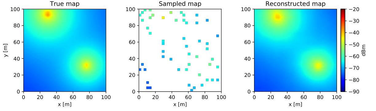In the application at hand and with the notation introduced in previous sections, the above expression becomes ${{\tilde{\bm{{\color[rgb]{0,0,0}\Psi}}}}}\approx{\color[rgb]{0,0,0}\delta}_{{\color[rgb]{0,0,0}\bm{w}}}({\color[rgb]{0,0,0}\epsilon}_{{\color[rgb]{0,0,0}\bm{w}}}({{\check{\bm{{\color[rgb]{0,0,0}\Psi}}}}}))$ .

As indicated earlier, autoencoders are useful only when most of the information in the input can be condensed in ${\color[rgb]{0,0,0}N_{\lambda}}$ variables, i.e., when the possible inputs lie close to a manifold of dimension ${\color[rgb]{0,0,0}N_{\lambda}}$ . To see that this is the case in spectrum cartography, an illustrating toy example is presented next. Suppose that there are two sources, each one with a fixed (yet possible different) power, that can be placed at arbitrary positions in $\mathcal{X}$ and suppose that propagation occurs in free space. All possible spectrum maps in this setup are defined by ${\color[rgb]{0,0,0}N_{\lambda}}=4$ quantities, which correspond to the x and y coordinates of the two sources. Fig. 2 illustrates this effect, where the left panel of Fig. 2 depicts a true map $\bm{{\color[rgb]{0,0,0}\Psi}}$ and the right panel shows its estimate using a completion autoencoder with ${\color[rgb]{0,0,0}N_{\lambda}}=4$ . The quality of the estimate clearly supports the aforementioned manifold hypothesis. Details about the network and simulation setup are provided in Sec. IV. In a real-world scenario, there may be more than two sources, their transmit power may not always be the same, and there are shadowing effects, which means that ${\color[rgb]{0,0,0}N_{\lambda}}\geq 4$ will be required. The rest of this section will describe the main aspects of the architecture developed in this work and summarized in Fig. 3.

Fig. 3: Autoencoder architecture.

TABLE I: Parameters of the proposed network.

Layers	Parameters
Conv2D/ Conv2DTranspose	Kernel size = $3\times 3$ , stride = 1, activation = PLReLU, 64 filters
AveragePooling2D	Pool size = 2, stride = 2
Upsampling2D	Up-sampling factor = $2$ , bilinear interpolation
Dense	64 neurons (encoder), 1024 neurons (decoder)

The encoder mainly comprises convolutional and pooling layers. The motivation for convolutional layers is three-fold: (i) relative to fully connected layers, they severely reduce the number of parameters to train and, consequently, the amount of data required. Despite this drastic reduction, (ii) convolutional layers are still capable of exploiting the spatial structure of maps and (iii) they result in shift-invariant transfer functions, a desirable property in the application at hand since moving the sources in a certain direction must be corresponded by the same movement in the estimated map. These layers compute

\displaystyle[{{\color[rgb]{0,0,0}\bm{\Phi}}}^{(O)}]_{i,j,{{\color[rgb]{0,0,0}c_{\text{out}}}}}=\sum_{{{\color[rgb]{0,0,0}c_{\text{in}}}}=1}^{{\color[rgb]{0,0,0}C_{\text{in}}}}\sum_{u=-k}^{k}\sum_{v=-k}^{k}[\bm{F}_{{\color[rgb]{0,0,0}c_{\text{out}}}}]_{u,v,{{\color[rgb]{0,0,0}c_{\text{in}}}}}[{{\color[rgb]{0,0,0}\bm{\Phi}}}^{(I)}]_{i-u,j-v,{{\color[rgb]{0,0,0}c_{\text{in}}}}},

where ${{\color[rgb]{0,0,0}\bm{\Phi}}}^{(O)}$ is the output tensor, ${{\color[rgb]{0,0,0}\bm{\Phi}}}^{(I)}$ is the input tensor, and $\bm{F}_{{\color[rgb]{0,0,0}c_{\text{out}}}}$ is the ${{\color[rgb]{0,0,0}c_{\text{out}}}}$ -th filter (or kernel), which is of size $2k+1\times 2k+1$ . Layer indices were omitted in order not to overload notation. The activation functions used here are parametric leaky rectified linear units (PLReLUs) [30] whose leaky parameter is also trained.

On the other hand, average pooling layers down-sample the outputs of convolutional layers, thereby condensing the information gradually in fewer features. Additionally, pooling features are approximately shift invariant as well [22, Ch. 9].

The last layer of the encoder is fully-connected. Since the previous layers were constrained to be convolutional or pooling layers, a final fully-connected layer is included in the encoder so that the latent variables can capture arbitrary relations among the shift invariant features obtained by the output of the second-to-last layer.

As usual in autoencoders, the decoder follows a “reverse” architecture relative to the encoder. Wherever the encoder has a convolutional layer, the decoder has a corresponding convolution transpose layer [31], sometimes called “deconvolutional” layer. Likewise, the pooling layers of the encoder are matched with up-sampling layers, which use bilinear interpolation in the architectures that we investigated. Finally, the fully connected layer of the encoder is paired with a fully connected layer in the decoder. The overall network architecture is summarized in Fig. 3 and Table I.

Fig. 5: Comparison with state-of-the-art alternatives. Even though the parameters of the competing algorithms were tuned for this specific experiment, the proposed network offers a markedly better performance.

Fig. 6: Performance comparison of the proposed scheme with that of the matrix completion algorithm in [32]. The number of grid points in

\mathcal{X}

N_{y}N_{x}=1024

IV Numerical Experiments

This section validates the proposed framework and network architecture through numerical experiments. Thus, $\mathcal{F}$ is set to the singleton $\mathcal{F}=\{900\text{ MHz}\}$ . $\mathcal{X}$ is a square area of side $100$ m, discretized into a grid with $N_{y}=N_{x}=32$ . The two considered transmitters have height 1.5 m and transmit power $11$ and $7$ dBm over a bandwidth of 5 MHz.

Two classes of maps are generated. First, $T=4\cdot 10^{5}$ maps are obtained where the two transmitters are placed uniformly at random and where propagation adheres to the Gudmundson model [33] with pathloss exponent 3, gain at unit distance $-30$ dB, and shadowing correlation $\mathop{\textrm{E}}\left\{H_{{\color[rgb]{0,0,0}s}}(\bm{x}_{1},f)H_{{\color[rgb]{0,0,0}s}}(\bm{x}_{2},f)\right\}=\sigma_{\text{sh}}^{2}0.95^{||\bm{x}_{1}-\bm{x}_{2}||}$ with $\sigma_{\text{sh}}^{2}=10$ dB². Sensors are distributed uniformly at random without replacement across the grid points. A separate set of maps is generated using Remcom’s Wireless InSite software in an urban scenario. Sensors are distributed uniformly at random without replacement across the grid points that lie on the streets. To better observe the impact of propagation phenomena, $\upsilon(\bm{x},f)$ is set to 0. Each measurement $\tilde{{\color[rgb]{0,0,0}\Psi}}({{\color[rgb]{0,0,0}\bm{\xi}}}_{i,j},f)$ is obtained by adding zero-mean Gaussian noise with standard deviation 1 dB to ${{\color[rgb]{0,0,0}\Psi}}({{\color[rgb]{0,0,0}\bm{\xi}}}_{i,j},f),~(i,j)\in\Omega$ .

The network proposed in Sec. III-D is implemented in TensorFlow and trained using the ADAM solver with learning rate $10^{-4}$ . In this work, one training approach is analyzed, in this case (5) with $\{({{\check{\bm{{\color[rgb]{0,0,0}\Psi}}}}}_{t},\bm{{\color[rgb]{0,0,0}\Psi}}_{t})\}_{t=1}^{T}$ the Gudmundson data set. The algorithm is compared against the state-of-the-art competitors described next, whose parameters were tuned to approximately optimize their performance in the second experiment. (i) The kriging algorithm in [1] with regularization parameter $10^{-5}$ and Gaussian radial basis functions with parameter $\sigma_{K}{:=}3\sqrt{{\Delta_{y}N_{y}\Delta_{x}N_{x}}/{|\Omega|}}$ , which is approximately 3 times the mean distance between two points at which measurements have been collected. (ii) The multikernel algorithm in [17] with 20 Laplacian kernels with parameter uniformly spaced between $[0.1\sigma_{K},\sigma_{K}]$ and regularization parameter $10^{-4}$ . (iii) The matrix completion via nuclear norm minimization in [32] with regularization parameter $10^{-5}$ . As a benchmark, (iv) the $K$ -nearest neighbors algorithm with $K=5$ is also shown.

The first experiment shows an estimated map using the proposed algorithm. The first panel of Fig. 4 depicts the true map, which was generated using the Remcom data set. The second panel shows ${\tilde{\bm{{\color[rgb]{0,0,0}\Psi}}}}$ whereas the third and fourth show map estimates using different numbers of measurements. Observe that with just $|\Omega|=52$ measurements, the estimate is already of a high quality. Note that details due to diffraction or the directivity of the antennas are not reconstructed because the Gudmundson model used to train the network does not capture them and therefore the network did not learn these features. This illustrates the need for training over data sets that model the reality as close as possible.

The second experiment compares the root mean square error $\text{RMSE}=\sqrt{{\mathbb{E}\{||\bm{{\color[rgb]{0,0,0}\Psi}}-\hat{\bm{{\color[rgb]{0,0,0}\Psi}}}||_{F}^{2}\}}/{(N_{y}N_{x})}},$ of the aforementioned algorithms, where ${\bm{{\color[rgb]{0,0,0}\Psi}}}$ is the true map, drawn at random from the Gudmundson data set, $\hat{\bm{{\color[rgb]{0,0,0}\Psi}}}$ is the estimated map, and $\mathbb{E}\{\cdot\}$ denotes expectation over maps, noise, and sensor locations. From Fig. 5, the proposed scheme performs approximately a 20 % better than the next competing alternative. The parameters of the competing algorithms were tuned for this specific experiment, so their performance as in Fig. 5 is optimistic. In practice one must expect a greater performance gap.

Due to poor performance of the matrix completion algorithm in [32] in the adopted range of $|\Omega|$ in the second experiment, the third experiment compares its RMSE with that of the proposed algorithm in another range of $|\Omega|$ where there exists a higher number of measurements. From Fig. 6, the proposed method clearly outperforms the scheme in [32] except when the number of measurements is very large, close to the total number of grid points.

V Conclusions

Learning propagation features from data yields spectrum cartography algorithms that require fewer measurements to attain a target performance. Deep neural networks can bring this idea into practice and offer a performance that beats the state-of-the-art. Future work will design more sophisticated network architectures relying on larger data sets.

References

[1] A. Alaya-Feki, S. B. Jemaa, B. Sayrac, P. Houze, and E. Moulines, “Informed spectrum usage in cognitive radio networks: Interference cartography,” in Proc. IEEE Int. Symp. Personal, Indoor Mobile Radio Commun., Cannes, France, Sep. 2008, pp. 1–5.
[2] J.-A. Bazerque and G. B. Giannakis, “Distributed spectrum sensing for cognitive radio networks by exploiting sparsity,” IEEE Trans. Signal Process., vol. 58, no. 3, pp. 1847–1862, Mar. 2010.
[3] B. A. Jayawickrama, E. Dutkiewicz, I. Oppermann, G. Fang, and J. Ding, “Improved performance of spectrum cartography based on compressive sensing in cognitive radio networks,” in Proc. IEEE Int. Commun. Conf., Budapest, Hungary, Jun. 2013, pp. 5657–5661.
[4] N. Patwari and P. Agrawal, “Effects of correlated shadowing: Connectivity, localization, and RF tomography,” in Int. Conf. Info. Process. Sensor Networks, St. Louis, MO, Apr. 2008, pp. 82–93.
[5] D. Romero, Donghoon Lee, and G. B. Giannakis, “Blind radio tomography,” IEEE Trans. Signal Process., vol. 66, no. 8, pp. 2055–2069, 2018.
[6] S. Grimoud, S. B. Jemaa, B. Sayrac, and E. Moulines, “A REM enabled soft frequency reuse scheme,” in Proc. IEEE Global Commun. Conf., Miami, FL, Dec. 2010, pp. 819–823.
[7] E. Dall’Anese, S.-J. Kim, G. B. Giannakis, and S. Pupolin, “Power control for cognitive radio networks under channel uncertainty,” IEEE Trans. Wireless Commun., vol. 10, no. 10, pp. 3541–3551, Aug. 2011.
[8] D. Romero, S-J. Kim, G. B. Giannakis, and R. López-Valcarce, “Learning power spectrum maps from quantized power measurements,” IEEE Trans. Signal Process., vol. 65, no. 10, pp. 2547–2560, May 2017.
[9] G. Boccolini, G. Hernandez-Penaloza, and B. Beferull-Lozano, “Wireless sensor network for spectrum cartography based on kriging interpolation,” in Proc. IEEE Int. Symp. Personal, Indoor Mobile Radio Commun., Sydney, NSW, Nov. 2012, pp. 1565–1570.
[10] S.-J. Kim, N. Jain, G. B. Giannakis, and P. Forero, “Joint link learning and cognitive radio sensing,” in Proc. Asilomar Conf. Sig., Syst., Comput., Pacific Grove, CA, Nov. 2011, pp. 1415 –1419.
[11] S.-J. Kim and G. B. Giannakis, “Cognitive radio spectrum prediction using dictionary learning,” in Proc. IEEE Global Commun. Conf., Atlanta, GA, Dec. 2013, pp. 3206 – 3211.
[12] D.-H. Huang, S.-H. Wu, W.-R. Wu, and P.-H. Wang, “Cooperative radio source positioning and power map reconstruction: A sparse Bayesian learning approach,” IEEE Trans. Veh. Technol., vol. 64, no. 6, pp. 2318–2332, Aug. 2014.
[13] G. Ding, J. Wang, Q. Wu, Y.-D. Yao, F. Song, and T. A Tsiftsis, “Cellular-base-station-assisted device-to-device communications in TV white space,” IEEE J. Sel. Areas Commun., vol. 34, no. 1, pp. 107–121, Jul. 2016.
[14] M. Hamid and B. Beferull-Lozano, “Non-parametric spectrum cartography using adaptive radial basis functions,” in Proc. IEEE Int. Conf. Acoust., Speech, Sig. Process., New Orleans, LA, Mar. 2017, pp. 3599–3603.
[15] Y. Teganya, D. Romero, L. M. Lopez-Ramos, and B. Beferull-Lozano, “Location-free spectrum cartography,” IEEE Trans. Signal Process., vol. 67, no. 15, pp. 4013–4026, Aug. 2019.
[16] J.-A. Bazerque, G. Mateos, and G. B. Giannakis, “Group-lasso on splines for spectrum cartography,” IEEE Trans. Signal Process., vol. 59, no. 10, pp. 4648–4663, Oct. 2011.
[17] J.-A. Bazerque and G. B. Giannakis, “Nonparametric basis pursuit via kernel-based learning,” IEEE Sig. Process. Mag., vol. 28, no. 30, pp. 112–125, Jul. 2013.
[18] S.-J. Kim, E. Dall’Anese, and G. B. Giannakis, “Cooperative spectrum sensing for cognitive radios using Kriged Kalman filtering,” IEEE J. Sel. Topics Sig. Process., vol. 5, no. 1, pp. 24–36, Jun. 2010.
[19] D. Lee, D. Berberidis, and G. B. Giannakis, “Adaptive Bayesian channel gain cartography,” in Proc. IEEE Int. Conf. Acoust., Speech, Sig. Process., Calgary, Canada, Apr. 2018, pp. 3555–3558.
[20] P. Stoica and R. L. Moses, “Spectral analysis of signals,” 2005.
[21] D. P. Mandic and J. Chambers, Recurrent neural networks for prediction: learning algorithms, architectures and stability, John Wiley & Sons, Inc., 2001.
[22] I. Goodfellow, Y. Bengio, and A. Courville, Deep learning, MIT press, 2016.
[23] D. Romero, D. Lee, and G. B. Giannakis, “Blind radio tomography,” IEEE Trans. Signal Process., vol. 66, no. 8, pp. 2055–2069, Apr. 2018.
[24] B. R. Hamilton, X. Ma, R. J. Baxley, and S. M. Matechik, “Propagation modeling for radio frequency tomography in wireless networks,” IEEE J. Sel. Topics Sig. Process., vol. 8, no. 1, pp. 55–65, Feb. 2014.
[25] J. Fan and T. Chow, “Deep learning based matrix completion,” Neurocomputing, vol. 266, pp. 540–549, Nov. 2017.
[26] V. Cherkassky and F. M. Mulier, Learning from Data: Concepts, Theory, and Methods, John Wiley & Sons, 2007.
[27] S. Iizuka, E. Simo-Serra, and H. Ishikawa, “Globally and locally consistent image completion,” ACM Trans. Graphics, vol. 36, no. 4, pp. 107, Jul. 2017.
[28] M. C Jeruchim, P. Balaban, and K. S. Shanmugan, Simulation of communication systems: modeling, methodology and techniques, Springer Science & Business Media, 2006.
[29] M. Ribeiro, A. E. Lazzaretti, and H. S. Lopes, “A study of deep convolutional auto-encoders for anomaly detection in videos,” Pattern Recognition Letters, vol. 105, pp. 13–22, Apr. 2018.
[30] K. He, X. Zhang, S. Ren, and J. Sun, “Delving deep into rectifiers: Surpassing human-level performance on imagenet classification,” in Proc. IEEE Int. Conf. Comput. Vision, Washington, DC, Dec. 2015, pp. 1026–1034.
[31] V. Dumoulin and F. Visin, “A guide to convolution arithmetic for deep learning,” arXiv preprint arXiv:1603.07285, 2016.
[32] G. Ding, J. Wang, Q. Wu, Y. Yao, F. Song, and T. A. Tsiftsis, “Cellular-base-station-assisted device-to-device communications in TV white space,” IEEE J. Sel. Areas Commun., vol. 34, no. 1, pp. 107–121, Jan. 2016.
[33] M. Gudmundson, “Correlation model for shadow fading in mobile radio systems,” Electron. Letters, vol. 27, no. 23, pp. 2145–2146, 1991.