Persistent current formation in double-ring geometries
Abstract
Quenching an ultracold bosonic gas in a ring across the Bose-Einstein condensation phase transition is known, and has been experimentally observed, to lead to the spontaneous emergence of persistent currents. The present work examines how these phenomena generalize to a system of two experimentally accessible explicitly two-dimensional co-planar rings with a common interface, or to the related lemniscate geometry, and demonstrates an emerging independence of winding numbers across the rings, which can exhibit flow both in the same and in opposite directions. The observed persistence of such findings in the presence of dissipative coupled evolution due to the local character of the domain formation across the phase transition and topological protection of the randomly emerging winding numbers should be within current experimental reach.
1 Introduction
At the critical point of a second order phase transition, the symmetry of a system is spontaneously broken, with both relaxation time and correlation length diverging [1]. In the transition region, the resulting state is not perfectly ordered, rather building a mosaic pattern of frozen coherent domains, with defects spontaneously emerging at their boundaries, thus becoming embedded within the system’s growing coherent global state. The study of emerging defect dynamics and their subsequent relaxation has been a topic of active research over the course of many years.
This effect was first discussed by Kibble in a cosmological context, setting an upper bound on the domain regions [2]. Zurek extended this by quantifying the emerging domain size on the basis of the universality of critical slowing down [1]. Consideration of the role of the quench timescale in finite-duration and linear quenches led to the universal Kibble-Zurek mechanism, which has been observed in a variety of complex systems [3], including liquid crystals [4], liquid helium [5, 6], superconducting loops [7, 8, 9, 10], ion chains [11], Bose-Einstein condensates (BECs) [12, 13, 14, 15, 16, 17, 18, 19, 20, 21], and, recently, in Rydberg lattices [22]. In ring geometries, like the original configuration considered by Zurek [1], the frozen phase of the wave function may lead to emergence of a supercurrent of integer topological charge , i.e. a phase winding along the ring. The focus of numerous previous studies has been to show how the supercurrent charge scales with the quench time through the phase transition [8, 9, 10, 17, 23, 24], thus verifying the applicability of the Kibble-Zurek scaling law. In particular, the numerical work of Ref. [23] provided a detailed visualization of, and highlighted, the role of local phase formation and subsequent evolution to a stable persistent current in the context of a one-dimensional model. Although such Kibble-Zurek scaling only applies to finite duration quenches, the underlying phenomenon of spontaneous symmetry breaking and generation of defects are at the heart of any crossing through a second-order phase transition, also including the numerically simpler instantaneous quenches, which provide crucial information for the formation dynamics of coherence in macroscopic systems and on the critical universal properties of the system.
Dynamical quenches (whether instantaneous or gradual) are in fact a critical ingredient of envisaged circuits in the emerging field of atomtronics, a highly-promising interdisciplinary field at the interface between matter-wave optics and the photonics/semiconductor technologies [25, 26], which has also been suggested as a potential platform for quantum-information devices, such as qubits [27]. The primary goal of atomtronics is to use the precise control, admitted by the ultracold quantum matter, to generate highly coherent circuits of neutral atoms, which are analogous to conventional solid-state systems, but with the potential to offer much improved and/or otherwise inaccessible technological applications [28, 29]. Available atomtronic circuits include, in particular, variable-resistance RLC schemes [30, 31, 32], Josephson-junction SQUIDs [33, 34, 35, 36], and diodes [37].
In this work, we explore the formation and structure of spontaneously generated supercurrents induced by an instantaneous crossing of the phase transition to the BEC state in a co-planar, side-by-side, double-ring geometry. This set-up has been chosen as a cold-atom analogue of a qubit made from adjacent superconducting loops, known as the Mooij-Harmans qubit [38, 39, 40]. Its operation relies on the use of coherent quantum-phase slips to coherently transport vortices through Josephson links. A theoretical proposal to implement this phenomenon in two-component quantum gases has been made [41], with Rabi coupling driving the phase slips with experimentally accessible spinor two-component gases [42] constituting a potential platform for such work. Gaining control over the tunnelling of persistent currents in a double-ring geometry would closer emulate the geometry of the original theoretical scheme. Recently, several proposals for two parallel/stacked rings have shown that the winding number can tunnel between rings due to the creation of fluxons at their boundary [43, 44], and at the single-particle level persistent current tunnelling has been predicted between arrays of adjacent rings and in similar configurations [45, 46, 47, 48].
The aim of this work is to explore the full two-dimensional (2D) formation dynamics of spontaneous supercurrents in such a side-by-side geometry, and demonstrate the resulting (perhaps somewhat counter-intuitive) independence of the two connected rings, despite their density overlap and coupled dynamics. After presenting our model, in the form of the commonly used stochastic projected Gross-Pitaevskii equation (SPGPE) in Sec. 2, we analyze the formation of persistent currents in the double-ring trap geometry (Sec. 3), and discuss the distribution of observable persistent-current states. We then explicitly demonstrate how the double-ring setting can be reduced to that for two independent 2D annuli (Sec. 4): doing so, we are able to draw analogies to Zurek’s arguments, and also demonstrate the extension of previous 1D SPGPE single-ring simulations to an explicitly 2D setting. Our findings for the double-ring structures are shown to be robustly insensitive to details of the geometry, by explicitly verifying the findings in the lemniscate (figure-of-eight) configurations in Sec. 5. Identifying regimes which are optimal for experimental observation paves the way for the use of such geometries for the design of potential qubit operations.
2 The theoretical model
Quench dynamics in quantum gases are well modelled by the above-mentioned stochastic (projected) GPE, which provides a numerically tractable effective field theory for low-lying ‘coherent’, or ‘classical’ modes of the system. First proposed in [49] to study the experimentally-observed reversible crossing of the BEC phase transition [50], it was developed independently with the addition a projection procedure in order to separate ‘coherent’ and ‘incoherent’ constituents of the dynamics [51, 52, 53, 54]. This approach has become the workhorse for modeling the condensate formation across different platforms [13, 20, 23, 55, 56, 57, 58, 59, 60, 61, 62, 63, 64, 65, 66, 67, 68, 69, 70, 71]. These include a number of simulations explicitly performed in a ring trap geometry [23, 62, 66], of direct relevance to the present analysis. Specifically, 1D SPGPE simulations by Das et al. [23], under controlled finite-duration quenches to condensation from noisy initial conditions, revealed very clearly the local character of the formation of phase, and its long-term dynamics leading to the spontaneous formation of persistent currents (in agreement with Kibble-Zurek). The same model was used to study spontaneous Josephson vortex formation across two linearly-coupled 1D ring traps [63]. In 2D rings, vortex decay and persistent-current formation were considered in the presence of external stirring [62], closely matching experimental data [72], while spontaneous emergence of persistent currents in 2D ring traps was discussed in Ref. [66], as a limiting factor in the study of controlled generation and stability of counter-propagating dark soliton pairs. As the SPGPE models the dynamics of the condensate and low-lying modes of the classical field , it does not include purely quantum effects like entanglement between persistent current states, which should be kept in mind when considering future atomtronic applications.
In our current implementation, building on our earlier works [20, 65, 70, 71], individual trajectories in the coherent sector of the dynamics are governed by the stochastic equation of motion [54],
| (1) |
describing their coupling to the incoherent sector, where
| (2) |
is the Gross-Pitaevskii operator, and is the atomic mass of atoms. Here, is the two-body interaction strength in the two-dimensional (2D) geometry, determined by the s-wave interaction strength , is the chemical potential, and is the transverse confinement scale imposed by the harmonic-oscillator trap . In our explicitly 2D study, we adopt tight transverse confinement Hz, in order to explicitly satisfy the quasi-2D condition . The complex Gaussian noise is characterized by correlations and , where is the bath temperature, is the growth rate, and the asterisk stands for the complex conjugate. In this work, we fix , and conclude via numerical testing that our steady-state results are insensitive to the exact value of , a statement which we have explicitly numerically confirmed here in the range , which constitute values consistent with both theoretical expectations [53, 54] and previous successful comparisons to experiments [20, 62, 70, 71]. Projector implements the energy cut-off, ensuring that the occupation of the largest included mode has average occupation of order unity. The energy cut-off is adopted as –derived by setting the Bose-Einstein distrubtion and solving for [73]– setting the spatial numerical grid for simulations with spacing [53]. The kinetic energy for a winding number around a ring of radius is given by , thus for the parameters we consider here the adopted energy cut-off limits the winding numbers to , far beyond the range we address in this work.
Focusing on experimentally relevant geometries for atoms (kg and ), we fix the chemical potential and temperature nK, chosen to be much lower than the critical temperature of the Berezinskii-Kosterlitz-Thouless (BKT) transition (in the thermodynamic limit) [74],
| (3) |
where [75]. In our parameter range, this amounts to , i.e. an essentially low-temperature setting.
To simulate the quench-induced dynamics, we simulated Eq. (1) using the software package XMDS [76], starting from initial condition , with a random realization of the initial noisy field , which is devoid of any phase coherence. This is akin to an input condition with atoms, all with the initial energy larger than the cut-off energy , which enter the cut-off region at a rate governed by until the gas reaches thermal equilibrium (actual values of are given below). This can be seen as an instantaneous thermal quench (cooling) from to nK. To confirm the broad validity of our findings, we have also explicitly verified that temperature quenches from pre-formed equilibrated 2D thermal clouds at temperatures (rather than from an initial noisy condition) yield the same qualitative findings and practically identical long-term winding number combinations (histograms; see subsequent Fig. 3(b)).
3 Instantaneous quench in the double-ring geometry
We consider the in-plane side-by-side double-ring (dr) configuration shown in Fig. 1(a). This structure is also known as the 2-torus. It is defined by the 2D potential
| (4) |
where , and the centres of the two rings with radius and width are set at
| (5) |
being a shift that separates the two side-by-side rings. The choice , for healing length , gives the rings 2D character and thus justifies the use of as a measure of critical temperature. Further, the height of the potential, , is fixed throughout the work. This potential is the double-ring extension of the single-ring trap used in Ref. [77]. However, as the 2-torus is not homeomorphic to the torus, due to the differing topology, one might expect the system dynamics within each section of the double-ring to be different from the single-ring case. We have verified that approximating the single-ring potential as , instead of the expression adopted in Eq. (4), does not conspicuously affect results presented below. Panel (i) in Fig. 1(a) shows potential (4) for m, m and , and the blue curve in (ii) shows a cross section along . These trap parameters are chosen to fit known experimental ranges, typically –m and –m [17, 78]. Experiments with even larger radii, reaching m, have been performed with time-averaged potentials; however the condensate was not coherent across the whole ring in this setup [79].
(a)

(b)

Following the instantaneous quench, the atomic density gradually grows to the equilibrium value, while the phase is relaxing to a steady-state configuration. The process is random, with each numerical run proceeding differently. Vortices, spontaneously created in the course of the growth of the condensate, eventually decay, potentially leaving a persistent current with winding numbers, and , in the left and right rings, respectively.
Figure 1(b) displays these dynamics, as the density equilibrates in panels (i)-(v), and the coalescence of the phase patterns is observed in (vi)-(x). For clarity’s sake, the phase plots are masked by the Heaviside function, , set at of the potential’s height, as shown by the gray shaded area in panel (ii) of Fig. 1(a). In this example, the final state evolves towards an equilibrium density with about atoms and with phase winding numbers , where we use the convention of positive winding numbers for clockwise circulation [62]. The temporal evolution of () is shown in blue (red) in Fig. 1(a)(iii), for a single numerical run. Each simulation leads to a random observation of winding numbers in the left and right rings, and we seek to quantify the effect that the presence of one ring has on the other through the stochastic distribution of these winding numbers. A movie of the time evolution for this example is provided as supplementary material to this work.

Extracting the winding number from the phase pattern is a two step-process. First, we apply high-pass filtering to the wave function in the momentum space, setting for , thus removing excitations with the spatial scale smaller than a healing length, , including sound waves, vortices, and thermal noise. Then, we extract the phase, , from the Madelung representation of the wave function, , at a radial distance , and count the number of jumps around the ring. An example is shown in Fig. 2(i)-(ii), where a clear jump is visible in the azimuthal phase of both rings. At early times the phase is random, as shown by the dotted and dashed lines, for both the azimuthal and radial phase profiles. At later times (after the thermalisation process) a smooth radial profile appears, whilst azimuthally the phase shows evidence of a phase winding of with a spatially varying gradient. The nonlinear gradient is evident in Fig. 2(i) around and (ii) around . As we will discuss, this effect is pronounced for larger winding numbers, and a more extreme example can be found in A and in the supplemental videos provided.
The code has been rigorously tested by manually imprinting persistent current states up to and comparing to the numerically obtained count. Of 10000 tests with varying degrees of numerical noise, none was counted incorrectly. Therefore we do not include any estimate of error in results that follow.
Experimentally, the winding number is usually measured through a variety of destructive techniques. In Ref. [80], a ring was populated by two hyperfine states of 87Rb, and the interference pattern between the rotating and non-rotating states was measured. A commonly employed method is to measure the size of the central hole after a time-of-flight expansion, either directly after removal of the trap [33, 77], or after transforming the ring trap into a simply connected sheet first, before turning off the trap [77, 80]. Recent advances in the application of this technique have been achieved by the inclusion of a small stationary BEC disk inside the annulus and measuring the interference pattern between the disk and annulus after the expansion [17, 24]. A minimally destructive technique has been employed to find the winding number through measuring the Doppler shift of standing phonon modes [81], allowing for repeated measurements in the course of one experiment. There is also a recent proposal to allow a small number of atoms tunnel into a linear waveguide adjacent to the ring to monitor the persistent current in time [82] (similar to the setup well known in optics, with a microring resonator coupled to a straight waveguide [83]).


We summarize results of the simulations by means of a 2D histogram of distributions of winding numbers for the double-ring geometry. To approximate the true winding number distribution, we have performed 5000 numerical runs, each with random initial noise. Figure 3(a) displays the result, which shows the probability of observing states with winding-number sets , white areas indicating states that were not produced by the simulations. The plots in (c)-(f) are examples of simulations contributing to particular points indicated on the histogram in (a). Highlighted are the states with winding-number sets . This histogram displays the supercurrent pairs measured at scaled time ms; in fact, panels (iii) in Figs. 3(c)-(f) show that stay constant at ms. The distribution of these winding numbers fits a bivariate normal form with no correlation between the left and right rings: this is seen through calculation of the sample Pearson correlation coefficient11 1 The sample Pearson correlation coefficient is defined as where is the probability of observing state , denotes the mean probability, and the the summation, with respect to index , is performed from to . with corresponding to an uncorrelated state, with our numerical data we find .
Despite the lack of correlation in the formation of persistent currents, an effect of the neighboring ring on the other one is still visible in velocity fields , seen in Fig. 3(ii) subplots. When the inter-ring shift in Eq. (5) is , the speed of atoms across the overlap region, where the two ring traps are abutting on each other, may be approximated by the relation
| (6) |
The validity of this relation is most easily observed in panel (ii) Fig. 3(d), with . The speed is clearly zero at the centre due to the counter-flow between the two rings; nevertheless, the total phase winding around each ring is still . We conclude that when, , atoms are quiescent at the centre due to the counter-flow. The atom fluxes flow along outside path, still maintaining the total phase winding around each ring.
However, when , there is a co-flow across the centre, with the speed doubled in the central reservoir. This scenario is shown in panel (ii) of Fig. 3(c), where the velocity for the case of is shown as a function of the angle around the ring. The velocity is indeed doubled across the overlap of the two rings, and correspondingly suppressed around the rest of the rings, such that values of the total phase windings are maintained in the system.
The atom flow for all other cases, with , leads to an exchange of atoms between the rings, determined by the magnitude of . Perhaps the most interesting case is displayed in panel (ii) of Fig. 3(f), where the supercurrent in the left ring remains zero, despite constantly exchanging atoms with the right counterpart. This is evidenced by the phase gradients present around the left ring, while the maintained total phase accumulation is zero.
The impact of these results is apparent when considering potential experimental measurements of the current. Destructive measurements are unlikely to be possible, given the close proximity of the two rings. However, the minimally destructive measurement techniques, currently applied to single-ring geometries, will be affected by the angular dependence of the velocity around each ring, shown in Fig. 3(ii). This will induce a spatial dependence on the Doppler shift of phonon modes [81] and the atom flux entering an adjacent linear waveguide [82].
3.1 Comparison to instantaneous thermal quenches
The use of a random noise initial condition is a numerically less demanding approximation to computing an instantaneous thermal quench. To justify our choice for the former, we compare the distribution obtained through a dynamical quench to that of one obtained from a random initial state. Performing a thermal quench simulation requires equilibrating to a thermal cloud with temperature nK, then instantaneously quenching to the target temperature nK at . As before, the winding numbers are measured at ms. Summing over the observed probabilities with fixed (or ) from the histogram yields a marginal distribution for (or ). Figure 3(b) shows that both methods produce practically identical results, and thus we choose to equilibrate from noise for the rest of this work. Error bars represent a 95% confidence interval containing the true probability, found by fitting with a Normal distribution.
4 Benchmarking against instantaneous quenches in a single ring
The observation of the formation of uncorrelated persistent currents in the two rings in both instantaneous quenches from noise or from a thermal initial state, despite the evident density overlap, suggests that such a distribution may in fact be explained in terms of well-known results for independent single-ring settings. In quenches from a noisy initial condition, this result might have been anticipated by extrapolation of the 1D findings of Das et al. [23], who highlighted the critical importance of local phase formation and evolution, over the global evolution around the ring. However in the present case, this was by no means a priori guaranteed for two reasons: firstly, the simulations in Ref. [23] were limited to an explicitly 1D ring, as opposed to the 2D rings numerically simulated here, which also account for the role of radial phase fluctuations (see Fig. 2 and movies); secondly, and most importantly, given that the 2-torus is not homeomorphic to the torus, the final results in the two cases need not be mappable onto each other. Indeed, while the overall distribution of winding numbers remains the same across the two non-homeomorphic cases, the actual azimuthal phase gradient is non-uniform in the case of the double ring, in stark contrast to the uniform phase gradient of a single ring. In the end, our explicit 2D numerical simulations confirm that the local character of phase evolution also dominates in the 2D case in the determination of the long-term winding number combinations across the two rings, while the short-term evolution is random.
To make a connection to the single-ring case, we consider a single ring, defined by potential
| (7) |
For ease of comparison, we keep here all parameters the same as in the previous section, and observe the distribution of winding numbers after an instantaneous quench in such a ring. In particular, for kept fixed, the arising atom number in the single trap is found to be . Our findings are presented in Fig. 4, showing explicitly the potential [panel 4(a)], and the equilibrium density at ms in panel (b).
The obtained distribution of winding numbers, , after 5000 numerical runs [Fig. 4(c)] reveals a (univariate) normal distribution , with within a 95% confidence interval; this is plotted as a red curve in the histogram of Fig. 4(c). There are several factors that can reduce the observed value of , including a trap’s tilt angle away from the azimuthal plane [23], a longer thermal quench time [17], and smaller chemical potentials [24].


Zurek’s original work considered how the thermal quench through a phase transition would leave behind a superfluid circulation in an annulus [1]. In the course of the phase transition, the condensate forms uniformly spaced, independent regions of coherent phase around the ring, with circumference and defect size . Taking [1] gives regions. Paraoanu derived [84] that for independent condensates with uniform phases, placed alongside one another, the maximum stable winding number is . Thus, for these parameters we would expect winding numbers , which is consistent with our finding of being the largest recorded winding number.
Further confidence in our methodology and presented numerical predictions is provided by explicitly comparing our numerical results to findings of a recent experiment with ultracold atoms on a single ring. Specifically, Corman et al. [17] considered finite-duration quenches on a quasi-2D ring, in a direct test of the Kibble-Zurek scaling law. Simulating such a finite-duration cooling quench protocol by means of the present scheme and starting from an initial thermal state, we obtain excellent agreement (see B).
To compare the results obtained in the framework of the double-ring geometry, to those considered in the single-ring geometry, we compare to the marginal distributions from Fig. 3. These results are practically identical to the distribution of the winding numbers for the single ring, as clearly seen in Fig. 4(d). We thus conclude that a robust property, inherent to each ring, is that, under quenched spontaneous condensate growth dynamics, the presence of the second ring does not alter the steady-state distributions of persistent currents in a given one, due to the prevailing importance of local phase formation and evolution even in a purely 2D setting. Despite the non-homeomorphic nature of the potentials, the close agreement between the final ‘steady-state’ results for the two rings and the single one is understood by the fact that the current is a topologically protected number associated with each ring (it may be thought of as having a ‘ghost’ vortex in the centre of the ring).
5 Dependence on the trap geometry


The robustness of the winding number can also be tested by replacing the two identical rings by the Bernoulli lemniscate, or figure-of-eight configuration [85]. It is defined by the in-plane potential
| (8) |
where and are described parametrically for as
| (9) |
The choice of an effective radius , where is the length from the origin to the foci, gives two rings of comparable radius to the work above.
The results corresponding to this geometry are shown in Fig. 5. Although the overlap area between the two ring-like structures is significantly different in this case, with flow from each ring structure in the central region directly passing through each other, we still observe that the winding numbers in each ring are completely uncorrelated. Although, in this geometry, the velocity fields show exchange of atoms between the two circulation loops, there is no transfer of persistent currents between them.
We also considered the case of a finite shift between the two coupled ring traps, i.e., in Eq. (5). In the case of co-flows (), patterns of the fluid flow are similar to those in the case of . However, for realizations exhibiting counter-flows () varying changes the interpretation of the flow circuit. At , the shear flow between the rings can create a vortex in the low-density overlap region, or several vortices, if the winding number is large enough. In this scenario, the Kelvin-Helmholtz instability may develop at the interface [86], as seen in simulations of the merger of two stacked rings with circulation [87, 88], see also [89]. An example of this for is shown in C.
All cases considered above uphold our conclusion that, in our geometry, the resulting winding numbers in both rings are produced by the random phase profiles spontaneously emerging in the course of the condensate growth, and the topological stability of the established states is maintained by the presence of persistent currents in each closed ring-shaped geometry.
6 Discussion
We have explored the spontaneous growth of persistent currents in a quenched 2D Bose gas in the co-planar side-by-side double-ring geometry. The emerging persistent currents are stable and long-lived, and do not transfer between the rings. The overall value of the winding number in each ring behaves independently, which can be directly attributed to the importance of the local nature of phase establishment in the azimuthal direction, an observation that remains valid even when allowing for radial random phase variations. While the distribution of winding numbers across the two rings can therefore be directly mapped onto the well-known results for the single-ring setting, it is important to note that the azimuthal phase gradient in each ring (for a given non-zero winding number) is not constant, in direct contrast to the constant phase gradient of the single ring case. This is more clearly visible in cases of large , examples of which are shown in A and movies of the real-time evolution of Figs. 1 and 6. This is one manifestation of the non-homeomorphism between a single torus and a 2-torus. Remarkably, however, this is not necessarily an impediment to potential future atomtronic devices, which could utilize the observed robust nature of the superfluid current configuration. The independence of the ring winding numbers and stability of the formed supercurrents may facilitate a well-controlled current transfer protocol between rings. Such deterministic transfer of winding numbers across multiple-loop atomtronic architectures is a promising direction for future research.
Varying the separation of the rings demonstrates the ability to modify the atom transfer between the rings and generate vortices between them. However, there is no sign of angular momentum transfer between the rings. The robustness of the persistent currents after the quench holds steadfast even against the change of trap geometry, such as replacement of the double ring by the lemniscate potential, where one might naïvely expect uncorrelated persistent currents in individual rings to be suppressed due to atomic motion along a“figure-of-eight” path. We also varied the phenomenological damping parameter in a broad range of values, and extended the simulation time, which produced no evidence of decay, confirming the efficiency of the topological protection of the spontaneously generated winding numbers.
A natural question suggested by the present results is the transfer of the winding numbers between the rings, which will be the subject of further work. The ability to control the transfer of winding numbers could be envisaged as a prototypical atomtronic switch, providing an avenue for controllable realization of coherent quantum phase slips required for the Mooij-Harmans qubit [38, 39]. A hot topic of current studies of toroidal BECs is the supercurrent decay mechanism, an understanding of which could help one to control the transfer of current states between the rings. The Gross-Pitaevskii equation and its many extensions [53, 54, 55] do not capture supercurrent decay, even at finite temperature, without an external barrier. However, due to roughness of the potential, the decay time for large winding numbers decay in experiments is on the order of seconds, whereas may be stable on times on the order of minutes [80]. Theoretical studies of the decay mechanism so far have all relied on effects along the annulus, caused by a repulsive barrier, the decay being visualized as vortices crossing the barrier region radially. In Ref. [90] it was shown that the temperature-induced decay does not fit the Caldeira-Leggett superconductivity model, i.e., the observed decay rate does not match simple models of quantum tunnelling and thermal activation of phase slips. Using a truncated Wigner approximation, Ref. [91] attributed some of the disagreements between the theory and experiment to thermal fluctuations, however exact identification of the decay mechanism remains an open question.
Data supporting this publication is openly available under an Open Data Commons Open Database License [92].
7 Acknowledgements
We would like to thank Fabrizio Larcher for his early involvement in this work. We thank I-Kang Liu, George Stagg and Jean Dalibard for discussions and Jérôme Beugnon for comments on the manuscript and providing us with the experimental data of Ref. [17]. TB thanks EPSRC Doctoral Prize Fellowship Grant No. EP/R51309X/1. We acknowledge financial support from the Quantera ERA-NET cofund project NAQUAS through the Engineering and Physical Science Research Council, Grant No. EP/R043434/1. The work of BAM who also acknowledges a Visiting Professorship held at Newcastle University is supported, in part, by the Israel Science Foundation through grant No. 1287/17.
Appendix A Nonlinear azimuthal phase gradient around the ring

We have shown that in co-planar two-ring geometries with large density overlap the phase gradient for a persistent current winding is not linear, but instead a function of the azimuthal angle around the ring. In Fig. 6 we illustrate this effect for the supercurrent combination . Crucially, the presence of the flow from the left ring is strong enough to reverse the direction of the flow in the right ring, as evidenced from the grey-shaded region pf overlap of the two rings. As explained in Sec. 3, this is possible due to the exchange of atoms between the rings. The time evolution of the density and phase (shown in the 2D plane, azimuthally and radially) can be seen in the supplemental material provided with this work.
Appendix B Comparison of experimental results and theoretical predictions
In 1985 Zurek considered how a thermal quench through a phase transition would leave behind a superfluid circulation in an annulus [1]. He postulated that during the phase transition the condensate forms independent regions of coherent phase around the ring, with circumference and defect size . In previous works, the resulting average winding number, calculated at the end of the thermal quench, has been shown to scale as
| (10) |
where we assume that the width of the ring is close to the defect’s size, [1].
B.1 Direct confirmation of Kibble-Zurek scaling for finite-duration quenches
In the related work of Das et al. [23] they tested the dependence of relation (10) on a linear temperature quench in time in an explicit 1D setting, and found excellent agreement. In this Appendix we carry out finite duration quenches from a high to a low temperature, in an explicitly 2D geometry, thus assessing the 2D nature through the radial width . In Fig. 7(a) it is seen that our analysis agrees with this prediction, indicating optimal experimental geometries for observing larger winding numbers. Specifically here we have chosen m and varied m using a finite duration quench with the ramp time s from an initial thermal state at nK () to nK ().
B.2 Comparison to experiment of Ref. [17]
Next we compare our results to the recent work by Corman et al. [17], which addressed temperature quenches with different ramp rates in the single-ring geometry with parameters m and m. We take to match the atom number . At the end of each temperature quench, the winding number was measured by turning off the trap potential and looking at the ensuing interference pattern, produced by the interplay of the ring with internal stationary disk. We have carried out simulations of one of those experiments, for the finite duration thermal quench from nK () down to nK (), with the ramp time s. The experiment was repeated times, with the aim to create a histogram of the resulting winding numbers. In Fig. 7 we compare the histograms representing the experimental findings and our numerical results (red and blue columns, respectively), the latter ones produced by simulations of the SPGPE. The figure demonstrates excellent agreement. Due to a relatively low number of experimental realizations, the respective histogram is not exactly symmetric about , although it features , confirming the stochasticity of the distribution. The experimentally produced average absolute winding number corresponding to this dataset is , while our simulations yield . The experiments did not feature winding numbers , while of our simulations yielded . It may be that still larger values are possible in this geometry, but with a probability . Comparing to the relation from Ref. [84], we expect that the maximum permitted value is , although this prediction does not account for the temperature ramp rate.
Appendix C Effect of finite ring separation distance on winding number histogram


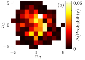

Addressing effects of the finite separation between the rings [ in Eq. (5)], in Fig. 8 we present results of simulations of the SPGPE with . The histogram of steady-state winding numbers does not display any significant difference from the case. This conclusion was verified by calculating the relative error between the two observed probability distributions, , the result being that the variation is . The correlation of the winding numbers between the two separated rings is still effectively zero (). Note that, in the limit of large , the rings become completely independent systems, for which the above results for the single ring are directly relevant.
For intermediate values of () the velocity fields are remarkably similar to those presented for . However, as stated in the main text, states with exhibit shear flow between the rings which may create vortices in the low density overlap region [86, 87, 88].
At the rings are spatially separated, with little density overlap. Recent works have found that, even in this case, the angular-momentum states (truncated to ) can couple to one another and tunnel, at the single-particle level [45, 46, 47, 48]. However, the nonlinearity in the Gross-Pitaevskii equation couples the setting to higher-order angular-momentum states, and destroys the simple picture. By tuning the nonlinearity to be negligible through the Feshbach resonance [93], it may be possible to create a superfluid state admitting tunnelling of angular-momentum states.
References
References
- [1] Zurek W H 1985 Nature 317 505
- [2] Kibble T W 1976 Journal of Physics A: Mathematical and General 9 1387
- [3] Kibble T 2007 Phys. Today 60 47
- [4] Chuang I, Durrer R, Turok N and Yurke B 1991 Science 251 1336–1342
- [5] Ruutu V, Eltsov V, Gill A, Kibble T, Krusius M, Makhlin Y G, Placais B, Volovik G and Xu W 1996 Nature 382 334
- [6] Bäuerle C, Bunkov Y M, Fisher S, Godfrin H and Pickett G 1996 Nature 382 332
- [7] Carmi R, Polturak E and Koren G 2000 Phys. Rev. Lett. 84 4966
- [8] Monaco R, Mygind J and Rivers R 2002 Phys. Rev. Lett. 89 080603
- [9] Monaco R, Mygind J and Rivers R J 2003 Phys. Rev. B 67 104506
- [10] Monaco R, Mygind J, Rivers R and Koshelets V 2009 Phys. Rev. B 80 180501
- [11] Ulm S, Roßnagel J, Jacob G, Degünther C, Dawkins S, Poschinger U, Nigmatullin R, Retzker A, Plenio M, Schmidt-Kaler F et al. 2013 Nat. Comm. 4 2290
- [12] Sadler L, Higbie J, Leslie S, Vengalattore M and Stamper-Kurn D 2006 Nature 443 312
- [13] Weiler C N, Neely T W, Scherer D R, Bradley A S, Davis M J and Anderson B P 2008 Nature 455 948
- [14] Lamporesi G, Donadello S, Serafini S, Dalfovo F and Ferrari G 2013 Nat. Phys. 9 656
- [15] Donadello S, Serafini S, Bienaimé T, Dalfovo F, Lamporesi G and Ferrari G 2016 Phys. Rev. A 94 023628
- [16] Navon N, Gaunt A L, Smith R P and Hadzibabic Z 2015 Science 347 167–170
- [17] Corman L, Chomaz L, Bienaimé T, Desbuquois R, Weitenberg C, Nascimbene S, Dalibard J and Beugnon J 2014 Phys. Rev. Lett. 113 135302
- [18] Chomaz L, Corman L, Bienaimé T, Desbuquois R, Weitenberg C, Nascimbène S, Beugnon J and Dalibard J 2015 Nat. Comm. 6 6162
- [19] Braun S, Friesdorf M, Hodgman S S, Schreiber M, Ronzheimer J P, Riera A, Del Rey M, Bloch I, Eisert J and Schneider U 2015 Proc. Natl. Acad. Sci. 112 3641–3646
- [20] Liu I K, Donadello S, Lamporesi G, Ferrari G, Gou S C, Dalfovo F and Proukakis N 2018 Commun. Phys. 1 24
- [21] Ko B, Park J W and Shin Y 2019 Nat. Phys. 15 1227
- [22] Keesling A, Omran A, Levine H, Bernien H, Pichler H, Choi S, Samajdar R, Schwartz S, Silvi P, Sachdev S, Zoller P, Endres M, Greiner M, Vuletić V and Lukin M 2019 Nat. Comm. 568 207
- [23] Das A, Sabbatini J and Zurek W H 2012 Scientific reports 2 352
- [24] Aidelsburger M, Ville J L, Saint-Jalm R, Nascimbène S, Dalibard J and Beugnon J 2017 Phys. Rev. Lett. 119(19) 190403 URL https://link.aps.org/doi/10.1103/PhysRevLett.119.190403
- [25] Seaman B, Krämer M, Anderson D and Holland M 2007 Phys. Rev. A 75 023615
- [26] Schlosser M, Tichelmann S, Kruse J and Birkl G 2011 Quantum Inf. Process 10 907
- [27] Aghamalyan D, Nguyen N, Auksztol F, Gan K, Valado M M, Condylis P, Kwek L C, Dumke R and Amico L 2016 New J. Phys. 18 075013
- [28] Amico L, Osterloh A and Cataliotti F 2005 Phys. Rev. Lett. 95 063201
- [29] Amico L, Birkl G, Boshier M and Kwek L C 2017 New J. Phys. 19 020201
- [30] Li A, Eckel S, Eller B, Warren K E, Clark C W and Edwards M 2016 Phys. Rev. A 94(2) 023626 URL https://link.aps.org/doi/10.1103/PhysRevA.94.023626
- [31] Eckel S, Lee J G, Jendrzejewski F, Lobb C J, Campbell G K and Hill W T 2016 Phys. Rev. A 93(6) 063619 URL https://link.aps.org/doi/10.1103/PhysRevA.93.063619
- [32] Gauthier G, Szigeti S S, Reeves M T, Baker M, Bell T A, Rubinsztein-Dunlop H, Davis M J and Neely T W 2019 Phys. Rev. Lett. 123 260402
- [33] Ramanathan A, Wright K, Muniz S R, Zelan M, Hill III W, Lobb C, Helmerson K, Phillips W and Campbell G 2011 Phys. Rev. Lett. 106 130401
- [34] Ryu C, Blackburn P, Blinova A and Boshier M 2013 Phys. Rev. Lett. 111 205301
- [35] Eckel S, Lee J G, Jendrzejewski F, Murray N, Clark C W, Lobb C J, Phillips W D, Edwards M and Campbell G K 2014 Nature 506 200
- [36] Mathey A C and Mathey L 2016 New J. Phys. 18 055016
- [37] Labouvie R, Santra B, Heun S, Wimberger S and Ott H 2015 Phys. Rev. Lett. 115(5) 050601 URL https://link.aps.org/doi/10.1103/PhysRevLett.115.050601
- [38] Mooij J and Harmans C 2005 New J. Phys. 7 219
- [39] Mooij J and Nazarov Y V 2006 Nat. Phys. 2 169
- [40] Astafiev O, Ioffe L, Kafanov S, Pashkin Y A, Arutyunov K Y, Shahar D, Cohen O and Tsai J 2012 Nature 484 355
- [41] Gallemí A, Mateo A M, Mayol R and Guilleumas M 2015 New J. Phys. 18 015003
- [42] Beattie S, Moulder S, Fletcher R J and Hadzibabic Z 2013 Phys. Rev. Lett. 110 025301
- [43] Richaud A and Penna V 2017 Physical Review A 96 013620
- [44] Oliinyk A, Yakimenko A and Malomed B 2019 J. Phys. B: At. Mol. Opt. Phys 52 225301
- [45] Polo J, Mompart J and Ahufinger V 2016 Phys. Rev. A 93 033613
- [46] Pelegrí G, Polo J, Turpin A, Lewenstein M, Mompart J and Ahufinger V 2017 Phys. Rev. A 95 013614
- [47] Pelegrí G, Marques A, Dias R, Daley A, Ahufinger V and Mompart J 2019 Phys. Rev. A 99 023612
- [48] Pelegrí G, Marques A, Dias R, Daley A, Mompart J and Ahufinger V 2019 Phys. Rev. A 99 023613
- [49] Stoof H T C and Bijlsma M J 2001 Journal of Low Temperature Physics 124 431–442 URL https://doi.org/10.1023/a:1017519118408
- [50] Stamper-Kurn D M, H-J Miesner, Chikkatur A P, Inouye S, Stenger J and Ketterle W 1998 Phys. Rev. Lett. 81 2194
- [51] Gardiner C W and Davis M J 2003 J. Phys. B: At. Mol. Opt. Phys 36 4731–4753
- [52] Bradley A S, Gardiner C W and Davis M J 2008 Phys. Rev. A 77(3) 033616 URL https://link.aps.org/doi/10.1103/PhysRevA.77.033616
- [53] Blakie P, Bradley A, Davis M, Ballagh R and Gardiner C 2008 Advances in Physics 57 363–455
- [54] Proukakis N P and Jackson B 2008 J. Phys. B: At. Mol. Opt. Phys 41 203002
- [55] Proukakis N, Gardiner S, Davis M and Szymańska M (eds) 2013 Quantum Gases: Finite Temperature and Non-Equilibrium Dynamics: 1 (Cold Atoms) (Singapore: World Scientific)
- [56] Proukakis N 2003 Las. Phys. 13 527
- [57] Proukakis N P, Schmiedmayer J and Stoof H T C 2006 Phys. Rev. A 73(5) 053603 URL https://link.aps.org/doi/10.1103/PhysRevA.73.053603
- [58] Cockburn S P and Proukakis N P 2009 Laser Physics 19 558–570
- [59] Zurek W H 2009 Phys. Rev. Lett. 102(10) 105702 URL https://link.aps.org/doi/10.1103/PhysRevLett.102.105702
- [60] Damski B and Zurek W H 2010 Phys. Rev. Lett. 104(16) 160404 URL https://link.aps.org/doi/10.1103/PhysRevLett.104.160404
- [61] Cockburn S P and Proukakis N P 2012 Phys. Rev. A 86(3) 033610 URL https://link.aps.org/doi/10.1103/PhysRevA.86.033610
- [62] Rooney S, Neely T, Anderson B and Bradley A 2013 Phys. Rev. A 88 063620
- [63] Su S W, Gou S C, Bradley A, Fialko O and Brand J 2013 Phys. Rev. Lett. 110(21) 215302
- [64] De S, Campbell D L, Price R M, Putra A, Anderson B M and Spielman I B 2014 Phys. Rev. A 89(3) 033631 URL https://link.aps.org/doi/10.1103/PhysRevA.89.033631
- [65] Liu I K, Pattinson R W, Billam T P, Gardiner S A, Cornish S L, Huang T M, Lin W W, Gou S C, Parker N G and Proukakis N P 2016 Phys. Rev. A 93(2) 023628 URL https://link.aps.org/doi/10.1103/PhysRevA.93.023628
- [66] Gallucci D and Proukakis N 2016 New J. Phys. 18 025004
- [67] Kobayashi, Michikazu and Cugliandolo, Leticia F 2016 EPL 115 20007 URL https://doi.org/10.1209/0295-5075/115/20007
- [68] Kobayashi M and Cugliandolo L F 2016 Phys. Rev. E 94(6) 062146 URL https://link.aps.org/doi/10.1103/PhysRevE.94.062146
- [69] Eckel S, Kumar A, Jacobson T, Spielman I B and Campbell G K 2018 Phys. Rev. X 8(2) 021021 URL https://link.aps.org/doi/10.1103/PhysRevX.8.021021
- [70] Ota M, Larcher F, Dalfovo F, Pitaevskii L, Proukakis N P and Stringari S 2018 Phys. Rev. Lett. 121(14) 145302 URL https://link.aps.org/doi/10.1103/PhysRevLett.121.145302
- [71] Comaron P, Larcher F, Dalfovo F and Proukakis N P 2019 Phys. Rev. A 100(3) 033618 URL https://link.aps.org/doi/10.1103/PhysRevA.100.033618
- [72] Neely T, Bradley A, Samson E, Rooney S, Wright E M, Law K, Carretero-González R, Kevrekidis P, Davis M and Anderson B P 2013 Phys. Rev. Lett. 111 235301
- [73] Rooney S, Bradley A and Blakie P 2010 Physical Review A 81 023630
- [74] Prokof’ev N, Ruebenacker O and Svistunov B 2001 Phys. Rev. Lett. 87 270402
- [75] Prokof’ev N and Svistunov B 2002 Phys. Rev. A 66 043608
- [76] Dennis G R, Hope J J and Johnsson M T 2013 Computer Physics Communications 184 201–208
- [77] Murray N, Krygier M, Edwards M, Wright K, Campbell G and Clark C W 2013 Phys. Rev. A 88 053615
- [78] Bell T A, Glidden J A, Humbert L, Bromley M W, Haine S A, Davis M J, Neely T W, Baker M A and Rubinsztein-Dunlop H 2016 New J. Phys. 18 035003
- [79] Sherlock B, Gildemeister M, Owen E, Nugent E and Foot C 2011 Phys. Rev. A 83 043408
- [80] Moulder S, Beattie S, Smith R P, Tammuz N and Hadzibabic Z 2012 Phys. Rev. A 86 013629
- [81] Kumar A, Anderson N, Phillips W, Eckel S, Campbell G and Stringari S 2016 New J. Phys. 18 025001
- [82] Safaei S, Kwek L C, Dumke R and Amico L 2019 Phys. Rev. A 100(1) 013621 URL https://link.aps.org/doi/10.1103/PhysRevA.100.013621
- [83] Poon J K, Scheuer J, Xu Y and Yariv A 2004 JOSA B 21 1665–1673
- [84] Paraoanu G S 2003 Phys. Rev. A 67(2) 023607 URL https://link.aps.org/doi/10.1103/PhysRevA.67.023607
- [85] This was suggested to us by J. Dalibard
- [86] Baggaley A and Parker N 2018 Phys. Rev. A 97 053608
- [87] Oliinyk A, Malomed B and Yakimenko A 2020 Communications in Nonlinear Science and Numerical Simulation 83 105113
- [88] Oliinyk A, Yatsuta I, Yakimenko A and Malomed B 2019 Symmetry 11 1312
- [89] Chen Z, Li Y, Proukakis N P and Malomed B A 2019 New Journal of Physics 21 073058
- [90] Kumar A, Eckel S, Jendrzejewski F and Campbell G K 2017 Phys. Rev. A 95 021602
- [91] Mathey A C, Clark C W and Mathey L 2014 Phys. Rev. A 90(2) 023604 URL https://link.aps.org/doi/10.1103/PhysRevA.90.023604
- [92] Newcastle University Data, http://dx.doi.org/10.25405/data.ncl.12012609
- [93] Stwalley W C 1976 Phys. Rev. Lett. 37 1628