Reduction of Qubits in Quantum Algorithm for Monte Carlo Simulation by Pseudo-random Number GeneratorPreprint: APS/123-QED

Applications of the quantum algorithm for Monte Carlo to high-dimensional integration in financial problems can be found in previous works, especially credit risk measurement in EggerEtAl. In the paper, independent random numbers necessary to obtain a value of integrand are represented by different quantum registers, so the number of required qubits $N_{\rm{qubit}}$ is proportional to the number of random numbers $N_{\rm{ran}}$. If $N_{\rm{ran}}$ is large as in the aforementioned cases, this can lead to shortage of qubits.

Let us see the method in more detail. The way to represent a random number by quantum register is as follows. For example, a qubit with state $\sqrt{1-p}\ket{0}+\sqrt{p}\ket{1}$ can be seen as a Bernoulli random number taking 1 with probability $p$. We can also represent a discretized approximation of a continuous random number like a normal random number on a quantum register Grover. Then, referring to these registers, the value of the integrand is computed into another register and its expectation value is estimated by methods such as Montanaro; Suzuki. Note that this procedure intends to make a superposition of all possible patterns of random numbers¹¹ 1 If a continuous random number is approximated discretely, ‘all patterns’ means those of the discretized value. and the integrand value and estimate the exact expectation value, which we hereafter write as $E_{\rm{true}}$.

In order to perform Monte Carlo enjoying quantum speed-up and reducing qubits, we first note that what we calculate in classical Monte Carlo is different from that in the quantum way. That is, we do not consider all patterns of random number values in the classical Monte Carlo. We sample only a part of patterns of the random numbers and the integrand and take a simple arithmetic average of the sampled integrand values as an approximation for $E_{\rm{true}}$. In other words, we calculate $E_{\rm{samp}}$, the expectation value under the sample space which consists of a part of samples and the probability measure under which equal probability is allocated to each sample. Besides, in most cases, we use a sequence of PRN on behalf of random numbers to calculate the integrand, since strict randomness is difficult to realize on a classical computer. More concretely, we usually generate a PRN sequence with $N_{\rm{samp}}N_{\rm{ran}}$ elements and divide them into $N_{\rm{samp}}$ subsequences with $N_{\rm{ran}}$ elements, then use each subsequence to calculate a sample value of the integrand²² 2 Mathematically, using such subsequences might raise a statistical concern for large $N_{\rm ran}$, in terms of homogeneity of the distribution of tuples of consecutive PRNs in a high dimensional space MT. However, such a way to use PRN is often adopted in practice in banks. We consider that using a tiny part in a large period PRN mitigates the concern Glasserman..

Our idea is that we estimate not $E_{\rm{true}}$ but $E_{\rm{samp}}$ using a quantum computer in the way similar to classical Monte Carlo. Before we describe the calculation flow in this method, let us state two assumptions necessary for it. The first assumption is that on the integrand. We assume that it takes $N_{\rm{ran}}$ random numbers as arguments and is sequentially computed in $N_{\rm{ran}}$ steps, each of which requires a random number and the output of the previous step as inputs. That is, using the intermediate functions $f_{n},n=1,...,N_{\rm ran}-1$, the value of the integrand $f_{N_{\rm{ran}}}$ for a given sequence $x_{1},...,x_{N_{\rm ran}}$ is calculated as

We also assume that $f_{N_{\rm{ran}}}$ is normalized so that $0\leq f_{N_{\rm{ran}}}(y,x)\leq 1$ for any $x,y$. Second, we assume that we can choose some PRNG which consumes $n_{\rm{PRN}}$ bits, including the random number itself and working space, and construct two types of quantum gate. One is $P_{\rm{PRN}}$, which progresses a PRN sequence by one step, that is³³ 3 Here and hereafter, a subscript of a ket basically denotes the qubit number of the register.,

where $x_{n}$ is the $n$-th element of the PRN sequence. The other is $J_{\rm{PRN}}$, which gives $x_{iN_{\rm ran}+1}$ for given $i$, that is,

where $n_{\rm{samp}}$ is an integer which satisfies $0<n_{\rm{samp}}<n_{\rm{PRN}}$. We show a concrete example of PRNGs which satisfies this assumption in section III.

Then, the calculation flow in our method is as follows. We take $N_{\rm{samp}}$, the number of samples, as $N_{\rm{samp}}=2^{n_{\rm{samp}}}$ for simplicity,

1. 1.

   Prepare a register $R_{\rm{samp}}$ with $n_{\rm{samp}}$ qubits and generate a superposition of $\ket{0},\ket{1},...,\ket{N_{\rm{samp}}-1}$ with equal amplitudes, that is, $\frac{1}{\sqrt{N_{\rm{samp}}}}\sum_{i=0}^{N_{\rm{samp}}-1}{\ket{i}_{n_{\rm{PRN}}}}$. This can be done by operating a Hadamard gate to each of the $n_{\rm{samp}}$ qubits.

2. 2.

   Operate $J_{\rm{PRN}}$, then the $(iN_{\rm{ran}}+1)$-th element of the sequence is set to the register $R_{\rm{PRN}}$, where $i$ is determined by the state of $R_{\rm{samp}}$. These are the starting points of subsequences.

3. 3.

   Perform a calculation step of the integral referring to $R_{\rm{PRN}}$ and reflect the result into a register $R_{\rm int}$. Here, we assume that the integrand is calculated step-by-step using each random number.

4. 4.

   Operate $P_{\rm{PRN}}$ to the register $R_{\rm{PRN}}$, then the PRN sequence progresses by one step.

5. 5.

   Perform a calculation step of the integral referring to $R_{\rm{PRN}}$ and reflect the result into a register $R_{\rm int}$.

6. 6.

   Iterate 4 and 5 until the calculation of the integrand ends. This corresponds to sequential generation of PRN and calculation using it. Finally, we obtain an equiprobable superposition of states, in each of which $R_{\rm{int}}$ holds a sampled integrand value.

7. 7.

   Prepare an ancilla qubit, which we call $R_{\rm ph}$, and encode the integrand value into the amplitude of $\ket{1}$ in $R_{\rm ph}$ using controlled rotations.

8. 8.

   Estimate the amplitude of the state where $R_{\rm ph}$ is $\ket{1}$ by the amplitude estimation methods like Bassard; Suzuki. This is an estimate for the arithmetic average of sampled integrand values, that is, $E_{\rm{samp}}$.

The flow of state transformation on $R_{\rm{samp}},R_{\rm{PRN}},R_{\rm{int}}$ and $R_{\rm ph}$ is as follows:

Here, $x^{(i)}_{n}=x_{iN_{\rm{ran}}+n}$ and this is the $n$-th element of the $i$-th subsequence. $n_{\rm{int}}$ is the qubit number of $R_{\rm{int}}$. $f^{(i)}_{1},..,f^{(i)}_{N_{\rm{ran}}}$ are the values of $f_{1},...,f_{N_{\rm{ran}}}$ for $x^{(i)}_{1},...,x^{(i)}_{N_{\rm ran}}$.

We present an outline of the quantum circuit for the above method in Figure 1. We also present that for the method in the previous papers for comparison. In our method, as shown in Figure 1, after the operation which create a superposition of $\ket{x^{(0)}_{1}},\ket{x^{(1)}_{1}},...,\ket{x^{(N_{\rm samp}-1)}_{1}}$ on $R_{\rm{PRN}}$ and the gate $f_{1}$, the first step of calculation of the integrand, we sequentially operate $P_{\rm{PRN}}$ and $f_{n}$, the $n$-th calculation step. The register which represents (pseudo) random numbers is only $R_{\rm{PRN}}$ and PRNs $x^{(i)}_{n}$ are sequentially generated on it. The intermediate value of the integrand $f^{(i)}_{n}$ is calculated into $R_{\rm{int}}$ using $x^{(i)}_{n}$ and $f^{(i)}_{n-1}$ as inputs and finally $f^{(i)}_{N_{\rm{ran}}}$ is reached. On the other hand, in the method in previous works, as shown in Figure 1, quantum registers $R_{{\rm RN},1},...,R_{{\rm RN},N_{\rm ran}}$ are prepared to represent all random numbers simultaneously and a superposition of numbers following the desired probability distribution (for example, normal) is generated on each register by the gate ’dist’ in Figure 1. Then, the integrand value is calculated using all of $R_{{\rm RN},1},...,R_{{\rm RN},N_{\rm ran}}$ at the same time.

Here we make some comments. The first one is about the probability distribution of random numbers. In the previous method, a random number under the desired distribution is generated on a register using the gate ’dist’. On the other hand, in the method of this paper, sequentially generated PRNs basically obey uniform distribution, since most PRNGs are for that distribution. Therefore, we have to convert uniform random numbers to random numbers obeying a desired distribution. Such a conversion is actually a common step in the classical Monte Carlo and there are many well-known methods, for example, the Box-Muller method for standard normal distribution. We assume such a conversion is implementable as a quantum gate and contained in $f_{n}$. Actually, implementation of trigonometric functions and logarithm, which are necessary to the Box-Muller method, has been investigated in previous papers Haner; Cao; Bhaskar.

The second comment is about how the distribution of the integrand value is taken into account in the method of this paper. In the previous method, the desired distribution of the integrand value is realized through the distribution of random numbers on registers. On the other hand, the distribution of the integrand value is generated through the PRNG in the method of this paper. Although the final state is a superposition of various integrand values with equal probability, the appearance pattern of the value reflects the distribution. For example, if the integrand value obeys distribution with a peak at some value $F$, the integrand values close to $F$ frequently appear on $R_{\rm{int}}$ in the set of states that compose the final superposition.

Finally, we comment on the integrand form such that it can be computed sequentially. As mentioned above, it is just an assumption, that is, not all functions can be written like this. However, in many cases, the integrand takes this form; for examples of use cases of Monte Carlo, see textbooks such as Glasserman. We here give two frequent cases which satisfy (1) and include some important problems. First, the integrand takes the form of (1) if, after fixing some random numbers, we can write contributions from remaining random numbers in a separable sum or product, that is, $f_{N_{\rm{ran}}}(x_{1},...,x_{N_{\rm ran}})=\sum_{j=d+1}^{N_{\rm{ran}}}g_{j}(x_{j};x_{1},...,x_{d})$ or $f_{N_{\rm{ran}}}(x_{1},...,x_{N_{\rm ran}})=\prod_{j=d+1}^{N_{\rm{ran}}}g_{j}(x_{j};x_{1},...,x_{d})$, where $d$ is a small natural number compared with $N_{\rm{ran}}$ and $g_{j},j=d+1,...,N_{\rm{ran}}$ are some functions. The credit portfolio risk measurement, which we will consider later, corresponds to this case. Second, when we simulate Markov processes, they can be calculated in the sequential way like above. Pricing of financial derivative, where the underlying assets are Markov in many cases, is a typical example of this. Thinking of these examples, we are well motivated to consider the case where (1) is satisfied.

Now, we roughly estimate the relationship between computational load and additive error in three methods: the quantum method we propose, the quantum method proposed in previous papers and the classical method. In this paper, we measure computational load by $N_{\rm orac}$, the number of times that we call the oracle in each method. Here, the oracle means the procedure to calculate the integrand. More concretely, it is the circuit (that in Figure 1, in the current case) and the subroutine to calculate the integrand for the quantum and classical method, respectively. In fact, in quantum methods, we have to repeatedly call the oracle circuit for amplitude estimation with the desired error level and this occupies the dominant part of the computation. On the other hand, the classical method requires the sufficient number of sampling to reduce the error and the computational time is almost proportional to the sample number.

First, let us consider our method. There are two sources of error. One is the difference between $E_{\rm samp}$ and $E_{\rm true}$, which we write as $\Delta_{\rm TrSm}$. The other is the estimation error of $E_{\rm samp}$, that is, the error of amplitude estimation, which we write as $\Delta_{\rm Est}$. $\Delta_{\rm TrSm}$ is equal to the statistical error in the classical Monte Carlo. For some fixed confidence level, it is at most $c\sigma_{f_{N_{\rm ran}}}N_{\rm samp}^{-1/2}=c\sigma_{f_{N_{\rm ran}}}2^{-n_{\rm{samp}}/2}$, where $\sigma_{f_{N_{\rm ran}}}$ is the standard deviation of $f_{N_{\rm ran}}$ and $c$ is a constant set according to the confidence level. Note that it depends on not $N_{\rm orac}$ but $n_{\rm{samp}}$. On the other hand, $\Delta_{\rm Est}$ is estimated as follows. The quantum algorithm in Bassard with $N_{\rm orac}$ oracle calls gives estimation for the amplitude (that is, $E_{\rm samp}$) which differs from the true value by at most $2\pi d\sqrt{E_{\rm samp}(1-E_{\rm samp})}N_{\rm orac}^{-1}$ with probability at least $1-\delta$. Here, we take only the leading term with respect to $N_{\rm orac}^{-1}$ and $d$ is some $O(1)$ constant depending only on $\log\delta$. In total, the error in our method is at most

If we desire the error level $\epsilon$, the following setting is sufficient. First, we set

or, equivalently,

so that $\Delta_{\rm TrSm}\sim\epsilon$. Then, we set

which leads to $\Delta_{\rm Est}\sim\epsilon$. Note that $N_{\rm orac}$ does not depend on $N_{\rm samp}$.

This is actually quadratic speed up compared with the classical Monte Carlo. In the classical method, the error is

as $\Delta_{\rm TrSm}$ in (5). Note that $N_{\rm orac}=N_{\rm samp}$ for the classical method. Then, the required $N_{\rm orac}$ in the method is

for the desired error $\epsilon$.

We also mention the error in the previous method of the quantum-based Monte Carlo. This method estimates $E_{\rm true}$ itself and the error is at most

for the oracle call number $N_{\rm orac}$. Note that this estimated error is nearly equal to $\Delta_{\rm Est}$ in (5). This is because the error of amplitude estimation is determined by the amplitude itself and $N_{\rm orac}$ only Bassard and the estimated amplitude is almost equal in both of the previous and our methods as long as $\Delta_{\rm TrSm}$ is small.

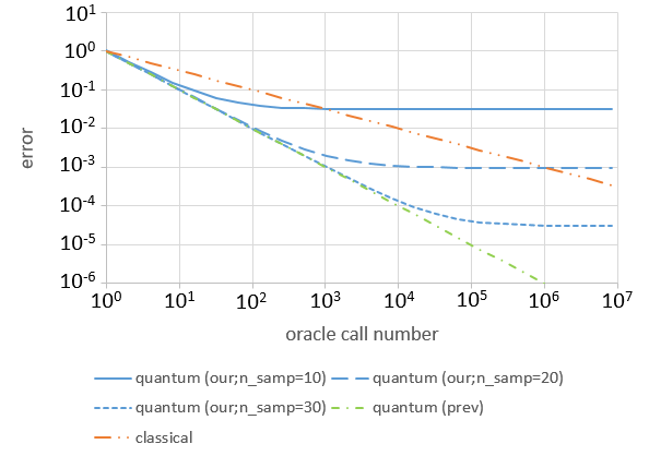
Figure 2 represents the relationship among these errors in some specific case. We plot $\Delta_{\rm our},\Delta_{\rm prev}$ and $\Delta_{\rm class}$ versus $N_{\rm orac}$. We here set the prefactors $c\sigma_{f_{N_{\rm ran}}},2\pi d\sqrt{E_{\rm samp}(1-E_{\rm samp})},2\pi d\sqrt{E_{\rm true}(1-E_{\rm true})}$ to 1. Besides, we set $n_{\rm samp}=10,20,30$, which correspond to $N_{\rm samp}=2^{10}(\approx 10^{3}),2^{20}(\approx 10^{6}),2^{30}(\approx 10^{9})$, respectively. $N_{\rm samp}=10^{6}$ is a typical value in the case of the credit risk measurement. When $\Delta_{\rm TrSm}\ll\Delta_{\rm Est},$ $\Delta_{\rm our}$ decreases faster than $\Delta_{\rm class}$ and similar to $\Delta_{\rm prev}$ as $N_{\rm orac}$ increases. After $\Delta_{\rm Est}$ becomes smaller than $\Delta_{\rm TrSm}$, $\Delta_{\rm our}$ asymptotically converges to $\Delta_{\rm TrSm}$. However, for sufficiently large $n_{\rm samp}$, $\Delta_{\rm our}$ reaches the same order of magnitude as $\Delta_{\rm class}$ for smaller $N_{\rm orac}$. For example, when $n_{\rm samp}\geq 20$, $\Delta_{\rm our}$ reaches the same order of magnitude as $\Delta_{\rm class}$ for $N_{\rm orac}=10^{6}$ only for $N_{\rm orac}=10^{3}$, smaller by three orders of magnitude. In such a region, our method has an advantage compared to the classical way.

We also note that increasing $n_{\rm{samp}}$ by a few leads to increase of $N_{\rm samp}$ and decrease of $\Delta_{\rm TrSm}$ by orders of magnitude. $N_{\rm ran}N_{\rm samp}$ cannot exceed $P$, the period of PRN, but we expect that it is unnecessary to concern such a upper bound, as long as we use a widely-used PRNG, which has a period, say $2^{64}$. At least in the case of the credit risk measurement, this is much longer than $N_{\rm ran}N_{\rm samp}$ in practice, since each of these is at most $10^{6}$ and the product is at most $10^{12}\sim 2^{40}$.

We next consider how to implement a PRNG on a quantum circuit, that is, the gates $P_{\rm PRN}$ and $J_{\rm PRN}$. Remembering the motivation of this work, reduction of qubits, PRNGs which require small working space are desirable. Besides, in order to decrease circuit depth as much as possible, we desire a simpler and shorter calculation step to progress PRN sequence. Of course, the longer period and better statistical property is preferred. We propose PCG PCG as a PRNG which satisfies these properties.

PCG is combination of linear congruential generator (LCG), a popular and elementary PRNG, and permutation of bit string. The $n$-th element of a PCG sequence $x_{n}$ is recursively defined as follows:

where $a,c$ and $m$ are integer parameters satisfying $a>0,c\geq 0,m>0$ and the seed $\tilde{x}_{0}$ is also given as an integer satisfying $0\leq\tilde{x}_{0}<m$. $\tilde{x}_{n}$ is the background sequence and defined by the LCG recurrence formula as above. $g$ is the permutation of a bit string, which is explained in detail later. Therefore, the calculation steps to progress a PCG sequence is the sequence of modular multiplication, modular addition and permutation. Besides, for LCG we can easily jump ahead by $k$ steps using the following formula:

Especially, we can obtain $\tilde{x}_{iN_{\rm ran}+1}$ from a seed $x_{0}$ as

Given the above formulas, we can construct quantum gates $P_{\rm PRN}$ and $J_{\rm PRN}$ for PCG. The rough images of the circuit diagrams are shown in Figure 3. To construct $P_{\rm PRN}$, we first get back PCG to LCG with the inverse of $g$, then progress LCG with the $f^{\rm prog}_{a,c,m}$ gate and finally perform the permutation $g$. The $f^{\rm prog}_{a,c,m}$ gate maps $\ket{x}$ to $\ket{f^{\rm prog}_{a,c,m}(x)}$ and is constructed as modular multiplication $\ket{x}\rightarrow\ket{ax\mod m}$ followed by modular addition $\ket{x}\rightarrow\ket{(x+c)\mod m}$. To construct $J_{\rm PRN}$, we first operate the $f^{\rm jump}_{a,c,m,\tilde{x}_{0},N_{\rm ran}}$ gate, which refers to the first register as an input and transforms the second register from $\ket{0}$ to $\ket{\tilde{x}_{iN_{\rm ran}+1}}$ if the first register is $\ket{i}$, then $g$ to the second register. The $f^{\rm jump}_{a,c,m,\tilde{x}_{0},N_{\rm ran}}$ gate is constructed as a combination of modular addition, subtraction, multiplication, division and exponentiation $\ket{k}\ket{x}\rightarrow\ket{k}\ket{a^{k}x\mod m}$. Implementation of (modular) adder, multiplier and exponentiator has been investigated in many papers, for example, Vedral; Beckman; Draper; Cuccaro; Takahashi; VanMeter; Draper2; Takahashi2; Portugal; AlvarezSanchez; Takahashi3; Thapliyal. Modular subtraction is the inverse of addition. Division by $a-1$ modulo $m$ is implemented as multiplication by an integer $b$ such that $(a-1)b\equiv 1\mod m$, which can be found by the extended Euclidean algorithm⁴⁴ 4 Such $b$ can be found if and only if $a-1$ and $m$ are coprime. This condition is satisfied for many of widely used combination of $a$ and $m$.Knuth.

There is a comment on implementation of $f^{\rm prog}_{a,c,m}$. It should be implemented not in the form that it output the result in the register other than the input register, that is, $\ket{x}\ket{0}\rightarrow\ket{x}\ket{f^{\rm prog}_{a,c,m}(x)}$, but in the form that it updates the input register itself into the resulting state, that is, $\ket{x}\rightarrow\ket{f^{\rm prog}_{a,c,m}(x)}$. This is because this gate is repeatedly used in the method of this paper, so the qubit number required for the entire calculation explodes if it is necessary to add a register in each calculation step. Most of the previous implementation of modular addition are the self-updating type, and so can be used with no change. On the other hand, some implementation of modular multiplication output the result into ancilla, $\ket{x}\ket{0}\rightarrow\ket{x}\ket{ax\mod m}$, but the trick described in Markov solves the problem as follows. First, using an integer $a^{\prime}$ such that $aa^{\prime}\equiv 1\mod m$, we construct a gate which performs $\ket{x}\ket{0}\rightarrow\ket{x}\ket{a^{\prime}x\mod m}$ and its inverse. Then, we can implement the following sequence:

Here, the first, second and third steps are modular multiplication by $a$, swap and the inverse of modular multiplication by $a^{\prime}$, respectively.

It is well-known that LCG suffers from some statistical flaws. PCG points out that performing permutation on LCG enhances its statistical properties. Here, permutation is transformation of binary representation of a PRN to another bit string. We here take some of the permutations described in PCG as examples and show how to implement them in a quantum circuit.

The first one is random rotation. We first divide a $n$-bit binary $x\in\mathbb{Z}_{2^{n}}$ into three parts: the top $t$ bits $x_{t}^{h}$, the middle $r$ bits $x_{r}^{m}$ and the bottom $n-t-r$ bits $x_{n-t-r}^{b}$, where $r$ is a power of 2 and $t=\log_{2}r$. Then random rotation is a map from $\mathbb{Z}_{2^{n}}$ to $\mathbb{Z}_{2^{r}}$ defined as

Here,

for an integer $k$ satisfying $0\leq k\leq r-1$, $y=y_{1}y_{2}...y_{r}\in\mathbb{Z}_{2^{r}}$ and $ab...$ represents a bit string whose first digit is $a\in\{0,1\}$, second digit is $b\in\{0,1\}$ and so on. In short, random rotation is clockwise rotation of middle digits of a binary where the rotation width is determined by the value of top digits. Only the middle digits $x_{r}^{m}$ are used to calculate the integrand as a $r$ bit random number. Especially, the bottom digits $x_{n-t-r}^{b}$ are discarded since their statistical properties are not good.

Random rotation is easily implemented in a quantum circuit using controlled swap gate (Fredkin gate). The circuit diagram is shown in Figure 4. The middle bits $\ket{x^{m}_{r}}_{r}$ is rotated by $2^{t-i}$ bits by ${\rm Rot}_{2^{t-i}}$ under the control of the top $i$-th bit, for $1\leq i\leq t$. This leads to $x_{t}^{h}$-bit rotation of $x_{r}^{m}$. We can construct the gate ${\rm Rot}_{2^{j}},j=0,1,...,t-1$ connecting qubits with swap gates (actually Fredkin gates since these gates are controlled) as follows. Setting $J=2^{j}$,

• •

  Connect $\ket{x_{t+(r/J-2)\cdot J+1}}$ and $\ket{x_{t+(r/J-1)\cdot J+1}}$, $\ket{x_{t+(r/J-3)\cdot J+1}}$ and $\ket{x_{t+(r/J-2)\cdot J+1}}$,…,$\ket{x_{t+1}}$ and $\ket{x_{t+J+1}}$

• •

  Connect $\ket{x_{t+(r/J-2)\cdot J+2}}$ and $\ket{x_{t+(r/J-1)\cdot J+2}}$,$\ket{x_{t+(r/J-3)\cdot J+2}}$ and $\ket{x_{t+(r/J-2)\cdot J+2}}$,…,$\ket{x_{t+2}}$ and $\ket{x_{t+J+2}}$

• •

  …

• •

  Connect $\ket{x_{t+(r/J-2)\cdot J+J}}$ and $\ket{x_{t+(r/J-1)\cdot J+J}}$,$\ket{x_{t+(r/J-3)\cdot J+J}}$ and $\ket{x_{t+(r/J-2)\cdot J+J}}$,…,$\ket{x_{t+J}}$ and $\ket{x_{t+J+J}}$

That is, there are $J$ groups containing $n/J$ qubits connected by $n/J-1$ swap gates. Note that $r/J$ is an integer.

The second type of permutation is xorshift. This is a map from $\mathbb{Z}_{2^{n}}$ to $\mathbb{Z}_{2^{n}}$ defined as follows:

Here, $s$ is an integer satisfying $1\leq s\leq n-1$ and typically comparable with $n$, for example, $n/2$ as proposed in PCG. Note that we do not need to take xorshift over the whole qubits in the PRN register. That is, we can take XOR between top qubits and middle qubits and discard bottom ones, as random rotation.

We can construct a gate which performs this permutation using CNOT gates. That is, put NOT on $\ket{x_{n-s+i}}$ under control by $\ket{x_{i}}$, for $i=1,...,s$, as shown in Figure 5. Note the order to set CNOT gates, that is, from bottom to top. This is necessary in the case where $s>n/2$ so that some middle qubits are used as both a target and a control. Such a qubit must work as a control before it becomes a target.

Here, we roughly estimate qubit number and depth of PCG circuits. We focus on $P_{\rm PRN}$, which is repeatedly used to progress PRN sequences. We consider PCG with $r$-bit output and $n$-bit background LCG. $n$ should be so large that the period, $2^{n}$ at most, is long enough and $r$ is typically comparable with $n$. For example, in many of the settings considered in PCG, $n=64$ and $r=32$.

The LCG part consists of modular addition and multiplication and dominant contribution comes from the latter. For $n$-bit operands, many of the proposed modular adder require $O(n)$ qubits including ancilla and $O(n)$ depth. On the other hand, modular multipliers basically require $O(n)$ qubits and $O(n^{2})$ depth, so this is dominant in the LCG part⁵⁵ 5 There are implementations which have depth proportional to smaller powers of $n$ than 2 but require ancilla proportional to larger powers of $n$ than 1 Portugal..

The permutation part does not require any ancillas; at least two examples are mentioned above. Circuit depth is found as follows. For random rotation on $r$ bits with $t=\log_{2}r$ control bits, which we considered above, we first note that depth of swap gates in ${\rm Rot}_{2^{j}}$ is $r/2^{j}-1$, since ${\rm Rot}_{2^{j}}$ consists of $2^{j}$ groups of $r/2^{j}$ qubits and $r/2^{j}-1$ swap gates, as explained above. Summing this up for $j=0,1,...,t-1$, it is found that the depth of Fredkin gates in the random rotation is $2r-\log_{2}{r}-2$, that is, $O(r)$. For xorshift with shift width $s$, it is obvious that the depth of CNOT gates is $s$ and if $s$ is comparable with $r$, say $s=r/2$ as considered in PCG, so is the depth.

In summary, in terms of both ancilla qubit number and circuit depth, dominant contribution comes from a multiplication and is $O(n)$ and $O(n^{2})$ respectively. Therefore, if each calculation step for integrand $f_{i}$ contains computations heavier than several multiplications, PRN generation makes subdominant contributions to qubit number and circuit depth.

Now, let us consider the application of the aforementioned method to the actual problem in finance. We take credit risk measurement, which is mentioned in the introduction, as an example. First, we briefly explain the Merton modelMerton, which is widely used in practice in many banks.

In this model, the stochastic loss amount $L$ in a credit portfolio consisting of $N_{\rm obl}$ obligors is given as follows:

The meaning of each symbol is as follows. $E_{i}$ is the exposure of the $i$ th obligor, that is, the loss arising if he defaults⁶⁶ 6 Here, we assume that loss given default is 1.. ${\bf 1}_{C}$ is the indicator function, which is 1 if the condition $C$ is satisfied and 0 otherwise. The stochastic variable $Z_{i}$ is interpreted as “the value of the firm” for the $i$ th obligor. We consider that he defaults if $Z_{i}$ becomes smaller than a threshold $z_{i}$. Usually, given a probability of default $p_{i}$ exogenously, $z_{i}$ is set as $z_{i}=\Phi_{\rm SN}^{-1}(p_{i})$, where $\Phi_{\rm SN}$ is the distribution function for standard normal distribution and $\Phi_{\rm SN}^{-1}$ is its inverse. $Z_{i}$ is given as a linear combination of two independent standard normal random variables $\epsilon_{\rm com}$ and $\epsilon_{i}$. $\epsilon_{\rm com}$ is common for all obligors and called a systematic risk factor, which is interpreted as a factor reflecting the situation of macro economy⁷⁷ 7 Although we consider the case there is a single systematic risk factor, we can extend the model with multiple ones.. $\epsilon_{i}$ is called an idiosyncratic risk factor and represents the effect of the matters unique to the $i$ th obligor on his credit. We take the coefficient $\alpha_{i}$ such that $0<\alpha_{i}<1$; therefore, $Z_{i}$ is also standard normal. $\alpha_{i}$ determines the correlation between $Z_{i}$ for different obligors: the larger $\alpha_{i}$ means stronger correlation and a larger probability of simultaneous defaults of many obligors.

Then, we describe how to calculate credit risk measures using a PRNG on a quantum circuit. What we have to develop is the circuit which calculates stochastic loss amount $L$. Once we develop the circuit which creates a superposition of states in which the value of the loss is encoded in some register, we can estimate VaR and CVaR as explained in EggerEtAl. The difference between the way in this paper and those in previous works is how to create such a superposition.

Seeing (19), we notice that the loss $L$ can be written as a sum of contributions from each obligor and takes the form of (1) as mentioned above. More concretely, precomputing $\epsilon_{\rm com}$ and defining

we can calculate $L$ as

using PRNs $x_{1},...,x_{N_{\rm obl}}$ as $\epsilon_{1},...,\epsilon_{N_{\rm obl}}$. Here, $Y_{i}(\epsilon_{\rm com})=M_{\rm PRN}P_{i}(\epsilon_{\rm com})$, where

is the conditional probability that the $i$-th obligor defaults given $\epsilon_{\rm com}$ and $M_{\rm PRN}$ is the maximum number that the PRN can take.

The concrete calculation flow to obtain one sample value of $L$ is as follows:

1. 1.

   Generate a standard normal random variable and let it be $\epsilon_{\rm com}$.

2. 2.

   Set $i=1$ and $L=0$.

3. 3.

   Set the first elements of the PRN sequence $x_{1}$.

4. 4.

   Calculate $Y_{i}(\epsilon_{\rm com})$.

5. 5.

   Compare $x_{i}$ with $Y_{i}(\epsilon_{\rm com})$. If the former is smaller than the latter, update $L\leftarrow L+E_{i}$.

6. 6.

   If $i=N_{\rm obl}$, finish. Otherwise, progress the PRN sequence to get $x_{i+1}$, update $i\leftarrow i+1$ and go to 4.

The above flow is performed by the circuit in Figure 6. As explained in Section II, we first create a superposition of $\ket{x^{(1)}_{1}}_{n_{\rm PRN}},...,\ket{x^{(N_{\rm samp}-1)}_{1}}_{n_{\rm PRN}}$ on $R_{\rm PRN}$ using $H^{\otimes n_{\rm{samp}}}$ and $J_{\rm PRN}$. These are starting elements of PRN sequences. Besides, we create a superposition of $x$, that is, numbers which obey the standard normal distribution in the register $R_{x}$. This is done by the method described in Grover and depicted as the gate ’SN’ in Figure 6. Then, progressing the PRN sequence by $P_{\rm PRN}$, $L$ is sequentially calculated by $f_{1},...,f_{N_{\rm obl}}$.

In $f_{i}$, at first, $x$ is converted to $Y_{i}(x)$ by the gate $Y_{i}$⁸⁸ 8 In practice, parameters such as $p_{i}$ and $\alpha_{i}$ are not set for each obligor individually. Instead, obligors are grouped in terms of industry sector or rating and the same parameter values are given in obligors in each group. In such a case, it is not necessary to operate $Y_{i}$ for each $i$, but sufficient to operate once per group.. We here simply assume that such a gate exists. In Woerner; EggerEtAl, several ways to calculate such a function on a quantum computer are proposed, for example, linear approximation or piecewise polynomial approximation Haner. Then $x_{i}$ is compared with $Y_{i}(x)$ and an ancillary qubit is set to 1 if $x_{i}>Y_{i}(x)$. Such a comparator has been presented in Oliveira. With the control by the ancilla, $E_{i}$ is added to the loss register $R_{L}$. The controlled adder is also presented in previous papers, such as Vedral. Finally, the inverses of $Y_{i}$ and comparison are performed to uncompute $R_{x}$ and the ancilla.

References

- (1) A. Montanaro, “Quantum speedup of Monte Carlo methods”, Proc. Roy. Soc. Ser. A, 471, 2181 (2015)
- (2) S. Woerner et al., “Quantum risk analysis,” npj Quantum Information 5, 15 (2019)
- (3) D. J. Egger et al., ”Credit Risk Analysis using Quantum Computers”, arXiv:1907.03044
- (4) P. Rebentrost et al., ”Quantum computational finance: Monte Carlo pricing of financial derivatives”, Phys. Rev. A 98, 022321 (2018)
- (5) N. Stamatopoulos et al., ”Option Pricing using Quantum Computers”, Quantum 4, 291 (2020).
- (6) R. C. Merton, ”On the pricing of corporate debt: The risk structure of interest rates”, J. Finance, 29, 449 (1974)
- (7) G. Bassard et al., “Quantum amplitude amplification and estimation”, Contemporary Mathematics, 305, 53 (2002)
- (8) Y. Suzuki et al., “Amplitude Estimation without Phase Estimation”, arXiv:1904.10246
- (9) M. E. O’Neill, “PCG: A Family of Simple Fast Space-Efficient Statistically Good Algorithms for Random Number Generation”, Harvey Mudd College Computer Science Department Tachnical Report (2014); http://www.pcg-random.org/
- (10) M. Matsumoto et al., ”Mersenne Twister: A 623-dimensionally Equidistributed Uniform Pseudo-random Number Generator”, ACM Transactions on Modeling and Computer Simulation (TOMACS) 8, 1 , 3 (1998)
- (11) L. Grover et al., “Creating superpositions that correspond to efficiently integrable probability distributions”, arXiv:quant-ph/0208112
- (12) P. Glasserman, ”Monte Carlo Methods in Financial Engineering”, Springer (2003)
- (13) T. Haner et al., ”Optimizing Quantum Circuits for Arithmetic”, arXiv:1805.12445
- (14) Y. Cao et al., ”Quantum algorithm and circuit design solving the Poisson equation”, New J. Phys. 15, 013021 (2013)
- (15) M. K. Bhaskar et al., ”Quantum Algorithms and Circuits for Scientific Computing”, Quantum Information and Computation, 16(3&4), 0197 (2016)
- (16) V. Vedral et al., “Quantum Networks for Elementary Arithmetic Operations”, Phys. Rev. A 54, 147 (1996)
- (17) D. Beckman et al., ”Efficient networks for quantum factoring”, Phys. Rev. A, 54, 1034 (1996)
- (18) T. G. Draper, ”Addition on a quantum computer”, arXiv:quant-ph/0008033
- (19) S. A. Cuccaro et al., ”A new quantum ripple-carry addition circuit”, arXiv:quant-ph/0410184
- (20) Y. Takahashi et al., ”A linear-size quantum circuit for addition with no ancillary qubits”, Quantum Information and Computation, 5(6), 440–448 (2005)
- (21) R. Van Meter et al., ”Fast quantum modular exponentiation”, Phys. Rev. A 71(5), 052320 (2005)
- (22) T. G. Draper et al., ”A logarithmic-depth quantum carry-lookahead adder”, Quantum Information and Computation, 6(4), 351 (2006)
- (23) Y. Takahashi et al., ”Quantum addition circuits and unbounded fan-out”, Quantum Information and Computation, 10(9&10), 0872 (2010)
- (24) L. A. B. Kowada, R. Portugal and C. M. H. Figueiredo, ”Reversible Karatsubas algorithm”, J. Univ. Comput. Sci. 12, 499 (2006).
- (25) J. J. Alvarez-Sanchez et al., ”A quantum architecture for multiplying signed integers”, Journal of Physics: Conference Series, 128(1), 012013 (2008)
- (26) Y. Takahashi et al., ”A fast quantum circuit for addition with few qubits”, Quantum Information and Computation, 8(6), 636 (2008)
- (27) H. Thapliyal et al., “Design of Efficient Reversible Logic Based Binary and BCD Adder Circuits”, J. Emerg. Technol. Comput. Syst. 9, 17, 1 (2013)
- (28) D. E. Knuth, ”The Art of Computer Programming, Volume 2: Seminumerical Algorithms”, Addison-Wesley (1981)
- (29) I. L. Markov et al., “Constant-Optimized Quantum Circuits for Modular Multiplication and Exponentiation”, Quantum Information and Computation, 12(5&6), 0361 (2012)
- (30) D. S. Oliveira and R. Ramos, Quantum bit string comparator: circuits and applications, Quantum Computers and Computing 7, 17 (2007).
- (31) G. Aleksandrowicz et al. Qiskit: An open-source framework for quantum computing (2019); https://qiskit.org/
- (32) P. W. Shor, “Fault-tolerant quantum computation,” in Proceedings of the 37th Annual Symposium on Foundations of Computer Science, FOCS ’96 (IEEE Computer Society, Washington, DC, USA, 1996) pp. 56
- (33) A. Y. Kitaev, “Fault-tolerant quantum computation by anyons,” Annals of Physics 303, 2 (2003)
- (34) A. G. Fowler et al., “Surface codes: Towards practical large-scale quantum computation”, Phys. Rev. A 86, 032324 (2012)
- (35) A. G. Fowler et al., “Low overhead quantum computation using lattice surgery”, arXiv:1808.06709