Example-Guided Scene Image Synthesis using Masked Spatial-Channel Attention and Patch-Based Self-Supervision

Haitian Zheng Haofu Liao Lele Chen Wei Xiong Tianlang Chen Jiebo Luo Affiliation: University of Rochester Affiliation: {hzheng15, hliao6, lchen63, wxiong5, tchen45, jluo}@cs.rochester.edu

Abstract

Example-guided image synthesis has been recently attempted to synthesize an image from a semantic label map and an exemplary image. In the task, the additional exemplar image serves to provide style guidance that control the appearance of the synthesized output. Despite the controllability advantage, the previous models are designed on datasets with specific and roughly aligned objects. In this paper, we tackle a more challenging and general task, where the exemplar is an arbitrary scene image that is semantically unaligned to the given label map. To this end, we first propose a new Masked Spatial-Channel Attention (MSCA) module which models the correspondence between two unstructured scenes via cross-attention. Next, we propose an end-to-end network for joint global and local feature alignment and synthesis. In addition, we propose a novel patch-based self-supervision scheme to enable training. Experiments on the large-scale CCOO-stuff dataset show significant improvements over existing methods. Moreover, our approach provides interpretability and can be readily extended to other tasks including style and spatial interpolation or extrapolation, as well as other content manipulation.

1 Introduction

Figure 1: The inputs to style-consistent scene image generation is a structurally uncorrelated and semantically unaligned segmentation map (column 1) and a reference image (column 2) that constraints the style of the output. The corresponding reference segmentation map is also taken as input. In spite of the complexity of the task, our model can generate high-quality scene images with a consistent style with the reference image.

Conditional generative adversarial network (cGAN) conditionalGAN has recently made substantial progresses in realistic image synthesis. In cGAN, a generator $\hat{x}=\G(c)$ aims to output a realistic image $\hat{x}$ with a constraint implicitly encoded by $c$ . Conversely, a discriminator $\D(x,c)$ learns such a constraint from ground-truth pairs $\langle x,c\rangle$ by predicting if $\langle\hat{x},c\rangle$ is real or generated.

The current cGAN models spade; pix2pixhd; pix2pix for semantic image synthesis aim to solve the structural consistency constraint where the output image $x$ is required to be aligned to a semantic label map $c$ . The limitation of the above generative process is that the styles of the image outputs are inherently determined by the model and thus cannot be controlled by users. To provide desired controllability over the generated styles, previous studies example_cvpr18; example_cvpr19 impose additional constraints and allow more inputs to the generator: $\hat{x}_{2\rightarrow 1}=\G(z,c_{1},x_{2})$ , where $x_{2}$ is an exemplar image that guides the style of $c_{1}$ . However, previous studies are designed on datasets such as face liu2015deep; rossler2018faceforensics, dancing example_cvpr19 or street view yu2018bdd100k, where the input images usually contain similar semantics and the spatial structures of $y$ and $c_{x}$ are usually similar as well.

Different from the previous studies, we propose to address a more challenging example-guided scene image generation task. As shown in Fig. 1, given a semantic label map $c_{1}$ (column 1) and an arbitrary scene image $x_{2}$ (column 2) with its semantic map $c_{2}$ (column 3) as the input, the task aims to generate a new scene image $\hat{x}_{2\rightarrow 1}$ (column 4) that matches the semantic structure of $c_{1}$ and the scene style of $x_{2}$ . The challenge is that scene images have complex semantic structures as well as diversified scene styles, and more importantly, the inputs $c_{1}$ and $x_{2}$ are structurally uncorrelated and semantically unaligned. Therefore, a mechanism is required to better match the structures and semantics for coherent outputs, e.g., the tree styles can be applied to mountains but cannot be applied to sky.

In this paper, we propose a novel Masked Spatial-Channel Attention (MSCA) module (Section 3.2) to propagate features across unstructured scenes. Our module is inspired by a recent work doubleattention for attention-based object recognition, but we apply a new cross-attention approach to model the semantic correspondence for image synthesis instead. To facilitate example-guided synthesis, we further improve the module by including: i) feature masking for semantic outlier filtering, ii) multi-scaling for global and local feature processing, and iii) resolution extending for image synthesis. As a result, our module provides both clear physical meaning and interpretability for the example-guided synthesis task.

We formulate the proposed approach under an unified synthesis network for joint feature extraction, alignment and image synthesis. We achieve this by applying MSCA modules to the extracted features for multi-scale feature domain alignment. Next, we apply a recent feature normalization technique, SPADE spade on the aligned features to allow spatially-controllable synthesis. To facilitate the learning of this network, we propose a novel patch-based self-supervision scheme. As opposed to example_cvpr19, our scheme requires only semantically parsed images for training and does not rely on video data. We show that a model trained with this approach generalizes over scales and across different scene semantics.

Our main contributions include the following:

•

A novel masked spatial-channel attention (MSCA) module to propagate features for unstructured scenes.
•

An unified synthesis network for joint feature extraction, alignment and image synthesis.
•

A novel patch-based self-supervision scheme that requires only annotated images for training.
•

Experiments on COCO-stuff cocostuff dataset that show significant improvements over existing methods. Moreover, our model provides interpretability and can be extended to other tasks of content manipulation.

2 Related work

Generative Adversarial Networks. Recent years have witnessed the progresses of generative adversarial networks (GANs) gan for image synthesis. A GAN model consists of a generator and a discriminator where the generator serves to produce realistic images that cannot be distinguished from the real ones by the discriminator. Recent techniques for realistic image synthesis include modified losses wasserstein; lsgan; improved, model regularization sn, self-attention sagan; largescalegan, feature normalization stylegan and progressive synthesis progressivegan.

Image-to-Image translation (I2I). I2I translation aims to translate images from a source domain to a target domain. The initial work of Isola et al. pix2pix proposes a conditional GAN framework to learn I2I translation with paired images. Wang et al. pix2pixhd improve the conditional GAN for high-resolution synthesis and content manipulation. To enable I2I translation without using paired data, a few works cyclegan; liu2017unsupervised; munit; drit; pairedcyclegan apply the cycle consistency constraint in training. Recent works on photo-realistic image synthesis take semantic label maps as inputs for image synthesis. Specifically, Wang et al. pix2pixhd extend the conditional GAN for high-resolution synthesis, Chen et al. CRN propose a cascade refine pipeline. More recently, Park et al. spade propose spatial-adaptive normalization for realistic scene image generation.

Example-Guided Style Transfer and Synthesis. Example guided style transfer image_analogies; Image_quilting aims to transfer the style of an example image to a target image. More recent works gatys2016image; adaptive_instance_normalization; phototransfer; johnson2016perceptual; deep_image_analogy; feature_shuffle; pairedcyclegan; video_style_transfer; wct2 utilize deep neural network features to model and transfer styles. Several frameworks munit; huang2018multimodal; example_iclr19 perform style transfer via image domain style and content disentanglement. In addition, domain adaptation pairedcyclegan applies a cycle consistency loss to cross-domain style transformation.

More recently, example-guided synthesis example_cvpr18; example_cvpr19 is proposed to transfer the style of an example image to a target condition, e.g. a semantic label map. Specifically, Lin et al. example_cvpr18 apply dual learning to disentangle the style for guided synthesis, Wang et al. example_cvpr19 extract style-consistent data pairs from videos for model training. In addition, Park et al. spade adopt I2I networks to self-encoding versions for example-guided style transfer. Different from example_cvpr18; example_cvpr19; spade, we address spatial alignment of complex scenes for better style integration in multiple regions of an image. Furthermore, our patch-based self-supervision learning scheme does not require video data and is a general version of self-encoding.

Correspondence Matching for Synthesis. Finding correspondence is critical for many synthesis tasks. For instance, Siarohin et al. Deformable apply the affine transformation on reference person images to improve pose-guided person image synthesis, Wang et al. vid2vid use optical flow to align frames for coherent video synthesis. However, the affine transformation and optical flow cannot adequately model the correspondences between two arbitrary scenes.

The recent self-attention wang2018non; sagan can capture general pair-wise correspondences. However, self-attention is computationally intensive at high-resolution. Later, Chen et al. doubleattention propose to factorize self-attention for efficient video classification. Inspired by doubleattention, we propose an attention-based module named MSCA. It is worth noting MSCA is based on cross-attention and feature masking for spatial alignment and image synthesis.

3 Method

The proposed approach aims to generate scene images that align with given semantic maps. Differ from conventional semantic image synthesis methods pix2pix; pix2pixhd; spade, our model takes an exemplary scene as an extra input to provide more controllability over the generated scene image. Unlike existing exemplar-base approaches example_cvpr18; example_cvpr19, our model addresses the more challenging case where the exemplary inputs are structurally and semantically unaligned with the given semantic map.

Our method takes a semantic map $c_{1}$ , a reference image $x_{2}$ and its corresponding semantic map $c_{2}$ as inputs and synthesizes an image $\hat{x}_{2\shortrightarrow 1}$ which matches the style of $x_{2}$ and structure of $x_{1}$ using a generator $\G$ , $\hat{x}_{2\shortrightarrow 1}=\G(c_{1},x_{2},c_{2})$ . As shown in Fig. 2, the generator $\G$ consists of three parts, namely i) feature extraction ii) feature alignment and iii) image synthesis. In Sec. 3.1, we describe the first part that extracts features from inputs of both scenes. In Sec. 3.2, we propose a masked spatial-channel attention (MSCA) module to distill features and discovery relations between two arbitrarily structured scene. Unlike the affine-transformation stn and flow-base warping vid2vid, MSCA provides a better interpretability to the scene alignment task. In Sec. 3.3, we introduce how to use the aligned features for image synthesis. Finally, in Sec. 3.4, we propose a patch-based self-supervision scheme to facilitate learning.

Figure 2: Our generator consists of three steps, namely i) feature extraction, ii) spatial feature alignment, and iii) image synthesis. We elaborate each step in its corresponding section, respectively.

3.1 Feature Extraction

Taking an image $x_{2}$ and label maps $c_{1},c_{2}$ as inputs, the feature extraction module extracts multi-scale feature maps for each input. Specifically, the feature map $F^{(i)}_{x,2}$ of image $x_{2}$ at scale $i$ is computed by:

\displaystyle\begin{aligned} F^{(i)}_{x,2}=W^{(i)}_{x}\ast F_{\text{vgg}}^{(i)}(x_{2}),\quad\text{for $i\in\{0,\dots,L\}$},\end{aligned}

(1)

where $\ast$ denotes the convolution operation, $F_{\text{vgg}}^{(i)}$ denotes the feature map extracted by VGG-19 vgg at scale $i$ , and $W^{(i)}_{x}$ denotes a $1\times 1$ convolutional kernel for feature compression. $L$ is the number scales and we set $L=4$ in this paper.

For label map $c_{1}$ , its feature $F^{(i)}_{c,1}$ is computed by:

\displaystyle F^{(i)}_{c,1}=\begin{cases}\relu(W^{(i)}_{c}\ast c^{(i)}_{1})&\text{for $i=L$},\\ \relu(W^{(i)}_{c}\ast[\Uparrow(F^{(i+1)}_{c,1}),c_{1}^{(i)}])&\text{otherwise},\end{cases}

(2)

where $\Uparrow(\cdot)$ denotes $\times 2$ bilinear interpolation, $c^{(i)}_{1}$ denotes the resized label map, $W^{(i)}_{c}$ denotes a $1\times 1$ convolutional kernel for feature extraction, and operation $[\cdot,\cdot]$ denotes channel-wise concatenation. Note that as scale $i$ decreases from $L$ down to $0$ , the feature resolutions in Eq. 2 are progressively increased to match a finer label maps $c^{(i)}_{1}$ .

Similarly, applying Eq. 2 with the same weights to label map $c_{2}$ , we can extract its features $F^{(i)}_{c,2}$ :

\displaystyle F^{(i)}_{c,2}=\begin{cases}\relu(W^{(i)}_{c}\ast c^{(i)}_{2})&\text{for $i=L$}\\ \relu(W^{(i)}_{c}\ast[\Uparrow(F^{(i+1)}_{c,2}),c_{2}^{(i)}])&\text{otherwise}\end{cases}.

(3)

3.2 Masked Spatial-channel Attention Module

Figure 3: The spatial-channel attention module for feature alignment. Our module takes image features map

F^{(i)}_{x,2}

and segmentation features map

F^{(i)}_{c,1}

F^{(i)}_{c,2}

as inputs to output a new image feature map

F^{(i)}_{x,1}

that is aligned to condition

c_{1}

As shown in Fig. 3, taking the image features $F^{(i)}_{x,2}$ and the label map features $F^{(i)}_{c,1}$ , $F^{(i)}_{c,2}$ as inputs¹¹ 1 We assume spatial resolution at scale $i$ being $H\times W$ and channel size of $F^{(i)}_{x,2}$ , $F^{(i)}_{c,1}$ , $F^{(i)}_{c,2}$ being $N,M_{1},M_{2}$ , respectively. , the MSCA module generates a new image feature map $F^{(i)}_{x,1}$ that has the content of $F^{(i)}_{x,2}$ but is aligned with $F^{(i)}_{c,1}$ . We elaborate the detailed procedures as follows:

Spatial Attention. Given feature maps $F^{(i)}_{x,2},F^{(i)}_{c,2}$ of the exemplar scene, the module first computes a spatial attention tensor $\alpha^{(i)}\in{[0,1]}^{K\cdot H\cdot W}$ :

\displaystyle\begin{aligned} \alpha^{(i)}=\softmax_{2,3}(\phi^{(i)}\ast[F^{(i)}_{x,2},F^{(i)}_{c,2}]),\end{aligned}

(4)

with $\phi^{(i)}\in\mathbb{R}^{(N+M_{2})\cdot K}$ denoting a $1\times 1$ convolutional filter and $\softmax_{2,3}$ denoting a 2D softmax function on spatial dimensions $\{2,3\}$ . The output tensor contains $K$ attention maps of resolution $H\times W$ , which serve to attend $K$ different spatial regions on image feature $F^{(i)}_{x,2}$ .

Spatial Aggregation. Then, the module aggregates $K$ feature vectors from $F^{(i)}_{x,2}$ using the $K$ spatial attention maps of $\alpha^{(i)}$ from Eq. 4. Specifically, a matrix dot product is performed:

\displaystyle\begin{aligned} \bm{V}^{(i)}&=\bm{F}^{(i)}_{x,2}(\bm{\alpha}^{(i)})^{T},\end{aligned}

(5)

with $\bm{\alpha}^{(i)}\in[0,1]^{K\cdot HW}$ and $\bm{F}^{(i)}_{x,2}\in\mathbb{R}^{C\cdot HW}$ denoting the reshaped versions of $\alpha^{(i)}$ and $F^{(i)}_{x,2}$ , respectively. The output $\bm{V}^{(i)}\in\mathbb{R}^{C\cdot K}$ stores feature vectors spatially aggregated from the $K$ independent regions of $F^{(i)}_{x,2}$ .

Feature Masking. The exemplar scene $x_{2}$ may contain irrelevant semantics to the label map $c_{1}$ , and conversely, $c_{1}$ may contain semantics that are unrelated to $x_{2}$ . To address this issue, we apply feature masking on the output of Eq. 5 by multiplying $\bm{V}^{(i)}$ with a length- $K$ gating vector at each row:

\displaystyle\begin{aligned} \widetilde{\bm{V}}^{(i)}&=(\bm{V}^{(i)})^{T}\circ\mlp([\gap(F^{(i)}_{c,1}),\gap(F^{(i)}_{c,2})]),\end{aligned}

(6)

where $\mlp(\cdot)$ denotes a 2-layer MLP followed by a sigmoid function, $\gap$ denotes a global average pooling layer, $\circ$ denotes broadcast element-wise multiplication, and $\widetilde{\bm{V}}^{(i)}$ denotes the masked features. The design of feature masking in Eq. 6 resembles to Squeeze-and-Excitation SEnet. Using the integration of global information from label maps $c_{1}$ and $c_{2}$ , features are filtered.

Channel Attention. Given feature $F^{(i)}_{c,1}$ of label map $c_{1}$ , a channel attention tensor $\beta^{(i)}\in{[0,1]}^{K\cdot H\cdot W}$ is generated as follows:

\displaystyle\begin{aligned} \beta^{(i)}=\softmax_{1}(\psi^{(i)}\ast F^{(i)}_{c,1}),\end{aligned}

(7)

with $\psi^{(i)}\in\mathbb{R}^{M_{1}\cdot K}$ denoting a $1\times 1$ convolutional filter and $\softmax_{1}$ denoting a softmax function on channel dimension. The output $\beta^{(i)}$ serves to dynamically reuse features from $\widetilde{\bm{V}}^{(i)}$ .

Channel Aggregation. With channel attention $\beta^{(i)}$ computed in Eq. 7, feature vectors at $HW$ spatial locations are aggregated again from $\widetilde{\bm{V}}^{(i)}$ via matrix dot product:

\displaystyle\begin{aligned} \bm{F}^{(i)}_{x,1}&=\widetilde{\bm{V}}^{(i)}(\bm{\beta}^{(i)})^{T},\end{aligned}

(8)

where $\bm{\beta}^{(i)}\in\mathbb{R}^{K\cdot HW}$ denotes the reshaped version of $\beta^{(i)}$ . The output $\bm{F}^{(i)}_{x,1}\in\mathbb{R}^{N\cdot HW}$ represents the aggregated features at $HW$ locations. The output feature map $F^{(i)}_{x,1}$ is generated by reshaping $\bm{F}^{(i)}_{x,1}$ to size $N\times H\times W$ .

Remarks. Spatial attention (Eq. 4) and aggregation (Eq. 5) attend to $K$ independent regions from feature $F^{(i)}_{x,2}$ , then store the $K$ features into $\bm{V}^{(i)}$ . After feature masking, given a new label map $c_{1}$ , channel attention (Eq. 4) and aggregation (Eq. 8) combine $\widetilde{\bm{V}}^{(i)}$ at each location to compute a output feature map. As results, each output location finds its correspondent regional features or ignored via feature masking. In this way, the feature of example scene is aligned. Note that when $K=1$ and $\alpha^{(i)}$ is constant, the above operations is essentially a global average pooling. We show in experiment that $K=8$ is sufficient to dynamically capture visually significant scene regions for alignment.

Figure 4: Our patch-based self-supervision scheme performs self-reconstruction and cross-reconstruction for two-patches from the same image.

Multi-scaling. Both global color tone and local appearances are informative for the style-constraint synthesis. Therefore, we apply MSCA modules at all scales $i\in\{0,\dots,L\}$ to generate global and local features $F^{(i)}_{x,1}$ .

Refer to caption — Figure 5: Visual comparisons with SPADE_VAE, and ours ablation models. Example-guided scene synthesis is performed between two retrieved scenes (rows 1,2) and two arbitrary scenes (rows 3,4). Columns 1 to 3 (blue) depict depict the target label maps, exemplar label maps and the associated images, respectively. Columns 4 to 8 in (red) depict different methods and our model (Columns 8). Columns 9 and 10 (green) respectively depict original images from target label map and synthesized ground truth using wct2 in the *retrieved* dataset (top of Table 1). In comparison, our method clearly produces the most style-consistent (with the exemplar!) and visually plausible images.

3.3 Image Synthesis

The extracted features $F^{(i)}_{c,1}$ in Sec. 3.1 capture the semantic structure of $c_{1}$ , whereas the aligned features $F^{(i)}_{x,1}$ in Sec. 3.2 capture the appearance style of the example scene. In this section, we leverage $F^{(i)}_{c,1}$ and $F^{(i)}_{x,1}$ as control signals to generate output images with desired structures and styles.

Specifically, we adopt a recent synthesis model, SPADE spade, and feed the concatenation of $F^{(i)}_{x,1}$ and $F^{(i)}_{c,1}$ to the spatially-adaptive denormalization layer of SPADE at each scale. By taking the style and structure signal as inputs, spatially-controllable image synthesis is achieved. We refer readers to appendix for more network details of the synthesis module.

3.4 Patch-Based Self-Supervision

Training a synthesis model requires style-consistent scene pairs. However, paired scenes are hard to acquire. To overcome the issue, we propose a patch-based self-supervision scheme which enables training.

Our basic assumption is that if patches $x_{p}$ and $x_{q}$ come from the same scene, they share the same style. Consequently, using patch $x_{p}$ as exemplar, both $x_{p}$ and the other patch $x_{q}$ can be reconstructed, i.e. self-reconstruction and cross-reconstruction. More formally, we sample non-overlapping patches $\langle x_{p},c_{p}\rangle$ and $\langle x_{q},c_{q}\rangle$ at locations $p$ and $q$ from a same scene $\langle x,c\rangle$ . To enable training, four images are synthesized in one training step:

\displaystyle\begin{aligned} \hat{x}_{p\shortrightarrow p}&=\G(c_{p},x_{p},c_{p}),\\ \hat{x}_{p\shortrightarrow q}&=\G(c_{q},x_{p},c_{p}),\\ \hat{x}_{q\shortrightarrow p}&=\G(c_{p},x_{q},c_{q}),\\ \hat{x}_{q\shortrightarrow q}&=\G(c_{p},x_{p},c_{p}),\end{aligned}

(9)

and compared against groundtruths $x_{p},x_{q},x_{p},x_{q}$ . An illustrative example is shown in Fig. 4. Note that patches $x_{p},x_{q}$ do not necessary share the same semantics and our model is required to complete example-missing regions with reasonable content through learning. Our training objective is adopted from to spade. However, we apply pixel domain $\ell_{1}$ loss to encourage color consistency. In our implementation, the generation processes in Eq. 9 share the same feature extraction, spatial attention, channel attention computation to reduce memory footprint during training.

4 Experiments

Dataset Our model is trained on the COCO-stuff dataset cocostuff. It contains densely annotated images captured from various scenes. We remove indoor images and images of random objects from the training/validation set, resulting in $21,648$ /499 scene images for training/testing.

During training, we resize images to $512\times 512$ then crop two non-overlapping $256\times 256$ patches to facilitate patch-based self-supervision. The two patches are cropped either in the left and right halves of the $512\times 512$ image, or alternatively in the top and bottom halves.

The COCO-stuff dataset does not provide ground-truth for example-guided scene synthesis, i.e. two scene images with the exact same styles. To qualitatively evaluate model performances, we require a model to transfer the style from $x_{2}$ to $x_{1}$ , where $x_{2}$ is the test image and $x_{1}$ is the generated image, in three ways: i) duplicating: we use the test image itself to test self-reconstruction, ii) mirroring: $x_{1}$ is generated by horizontally mirroring $x_{2}$ , iii) retrieving: $x_{1}$ is generated by finding the best match from the larger image pool. Specifically, we generate 20 candidate images from the training set with the smallest label histogram intersections. Out of the 20 images, the best-matching image $x_{1}$ is generated using SIFT Flow siftflow. Finally, since the color of $x_{1}$ and $x_{2}$ are not the same, we apply wct2 on image $x_{1}$ for color correction. Examples of the retrieving pairs are shown in Fig. 5, in columns 3 and 10.

Methods	PSNR $\uparrow$	SSIM $\uparrow$	LPIPS $\downarrow$	FID $\downarrow$
retrieving
SPADE_VAE spade	15.62	0.39	0.480	89.77
ours GAP	15.77	0.39	0.456	89.55
ours MSCA w/o att	11.76	0.27	0.524	98.35
ours MSCA w/o fm	15.64	0.40	0.455	89.58
our full	15.98	0.40	0.449	85.87
mirroring
SPADE_VAE spade	15.72	0.39	0.478	89.58
ours GAP	16.06	0.39	0.446	89.54
ours MSCA w/o att	12.13	0.28	0.512	98.02
ours MSCA w/o fm	16.52	0.42	0.442	88.40
our full	16.95	0.42	0.425	83.20
duplicating
SPADE_VAE spade	15.35	0.38	0.476	90.69
ours GAP	15.70	0.38	0.438	88.51
ours MSCA w/o att	11.92	0.28	0.508	102.24
ours MSCA w/o fm	15.91	0.40	0.437	89.44
our full	16.50	0.40	0.420	84.93

Table 1: Quantitative comparisons of different methods in terms of PSNR, SSIM, LPIPS lpips and Fréchet Inception Distance (FID) fid. Higher scores are better for metrics with uparrow (

\uparrow

), and vice versa.

Figure 6: Style interpolation and traverse at test stage. We perform style traverse along path

\texttt{grass}\shortrightarrow\texttt{dessert}\shortrightarrow\texttt{forest}\shortrightarrow\texttt{night}

. Please refer to the Interpolation part in Sec. 4 for details.

Implementation Details The number of attention maps $K$ for MSCA modules are set to $8,16,16,16,16$ from scale $0$ to $4$ . The learning rate is set to $0.0002$ for the generator and the discriminator. The weights of generator are updated every $5$ iterations. We adopt the Adam adam optimizer ( $\beta_{1}=0.9$ and $\beta_{2}=0.999$ ) in all experiments. Our synthesis model and all comparative models are trained for $20$ epochs to generate the results in the experiments.

During implementation, we pretrain the spatial-channel attention with a lightweight feature decoder to avoid the ineffective but extremely slow updating of SPADE parameters. Specifically, at each scale, the concatenation of $F^{(i)}_{x,1}$ and $F^{(i)}_{c,1}$ in Sec. 3.3 at each scale is fed into a $1\times 1$ convolutional layer to reconstruct the ground-truth VGG feature at the corresponding scale. The pretraining takes around $4$ % of the total training time to converge. More details of the pretraining procedure is provided in the appendix.

Quantitative Evaluation We compare our approach with an example-guided synthesis approach: variational autoencoding SPADE (SPADE_VAE) spade which is based on a self-reconstruction loss for training. Therefore, we directly use the resized $256\times 256$ images to train the model. We also attempt to train two example-guided synthesis models example_cvpr18 and example_cvpr19 (example_cvpr19 is trained using patch-based self-supervision) but cannot achieve visually good results. We leave the result of example_cvpr18; example_cvpr19 in the appendix. In addition, three ablation models are evaluated (see Ablation Study).

For quantitative evaluation, we apply low-level metrics including PSNR and SSIM ssim, and perceptual-level metrics including Perceptual Image Patch Similarity Distance (LPIPS) lpips and Fréchet Inception Distance (FID) fid on different models. For LPIPS, we use the linearly calibrated VGG model (see lpips for details).

As shown in Table 1, our method clearly outperforms the remaining methods. Improvements in low-level and perceptual-level measurements suggest that our model better preserves color and texture appearances. We observe that the performances of various approaches on the retrieving dataset are worse and less differentiated than their counterparts on the mirroring and duplicating datasets. It suggests that the retrieving dataset is harder and noisier, as one cannot retrieve images that have the exact same styles. On retrieving dataset, our approach achieves a moderate +0.36 PSNR gain over SPADE_VAE (from 15.62 to 15.98). By contrast, our approach achieves visually superior results over SPADE_VAE on duplicating and mirroring, e.g. +1.15 PSNR gain (from 15.35 to 16.50) on duplicating and +1.23 PSNR gain (from 15.72 to 16.95) in PSNR on mirroring.

Qualitative Evaluation Fig. 5 qualitatively compares our model against the remaining models on two retrieved scenes (rows 1-2) and two arbitrary scenes (rows 3-4). Our model achieves better style-consistent example-guided synthesis. Remarkably, in rows 3-4, even though the two scenes have very different semantics (indicated by the different colors of the corresponding label maps), our model can still maintain the styles of the exemplars while maintaining the correct semantics of the target label maps, e.g. generating “snow” rather than “grass” in row 4.

Also notice that sometimes our results are more style-consistent than the synthesized ground truths (last column). This further shows that the existing style transfer approach styletransfer; wct2; phototransfer cannot be directly applied to exemplar-guided scene synthesis for satisfactory results.

Ablation Study To evaluate the effectiveness of our design, we separately train three variants of our model: i) our GAP that replaces the MSCA module with global average pooling, ii) our MSCA w/o att that keeps MSCA moduels but replaces spatial and channel attention of MSCA by one-hot label maps from source and target domains, respectively. In such way, alignment is performed on regions with the same semantic labeling, and iii) our MSCA w/o fm that keeps MSCA modules but removes the feature masking procedures. In Table 1 and Fig. 5, our model clearly achieves the best quantitative and qualitative results. In comparison, in Fig. 5, our GAP produces similar appearances in each region, as GAP cannot distinguish local appearances. Our w/o att is less stable in training and cannot generate plausible results. We hypothesize that the label-level alignment will generate more misaligned and noisier feature maps, thus hurts training. our MSCA w/o fm cannot perform correct appearance transformation, for instance, transferring “sky” to “snow” (Fig. 5, last row).

The Effect of Attention To understand the effect of spatial-channel attention, we visualize the learned spatial and channel attention in Fig. 7. We observe that: a) spatial attention can attend to multiple regions of the reference image. For each reference region, channel attention finds the corresponding target region. b) spatial-channel attention can detect and utilize the semantic similarities between segments to transfer visual features. In the top row of Fig. 7, attention in channels $1,4$ respectively perform transformations: $\texttt{sky\_other}\shortrightarrow\texttt{clouds}$ , $\texttt{tree}\shortrightarrow\texttt{\lx@text@lbrace tree, hill\lx@text@rbrace}$ . In the bottom row, attention in channels $1,2,7$ respectively perform transformations: $\texttt{clouds}\shortrightarrow\texttt{clouds}$ , $\texttt{snow}\shortrightarrow\texttt{sand}$ and $\texttt{other}\shortrightarrow\texttt{\lx@text@lbrace surfboard,other\lx@text@rbrace}$ .

Figure 8: Spatially interpolate two styles in a single image at test stage. The styles of the synthesized images are deliberately changed from left to right.

Interpolation We can easily control the synthesized styles in the test stage by manipulating attentions. Here, we show how to interpolate between two styles using our trained model: given two example images $x_{2}$ and $x_{3}$ , we first compute their image features $F^{(i)}_{x,2},F^{(i)}_{x,3}$ and the spatial-attention maps $\alpha^{(i)}_{2},\alpha^{(i)}_{3}$ . Given an interpolating factor $\alpha\in[0,1]$ where $\alpha=1$ means ignoring the example scene $x_{3}$ , the spatial attention map of the first scene is modified by $\alpha^{(i)}_{2}\coloneqq\alpha^{(i)}_{2}+\log(\frac{\alpha^{(i)}_{2}}{1-\alpha^{(i)}_{2}})$ . Afterwards, both feature maps $F^{(i)}_{x,2},F^{(i)}_{x,3}$ and spatial attention $\alpha^{(i)}_{2},\alpha^{(i)}_{3}$ are concatenated along the horizontal axis. In addition, the masking score (output of the 2-layer MLP in Eq. 6) is also interpolated. With the remaining procedures unchanged, i.e., same spatial aggregation, feature masking, channel aggregation and synthesis, interpolation results are readily generated. As shown in Fig. 6, with slight modifications, our model can perform effective style interpolation. Specifically, the style traverses along the path $\texttt{grass}\shortrightarrow\texttt{dessert}\shortrightarrow\texttt{forest}\shortrightarrow\texttt{night}$ is achieved in Fig. 6.

Likewise, by manipulating the channel attention at each spatial location, it is possible to adaptively mix style to synthesize an output image, i.e. spatial styles interpolation. As shown in Figure 8, using the previous input, we interpolate between styles from left to right in a single image.

Extrapolation

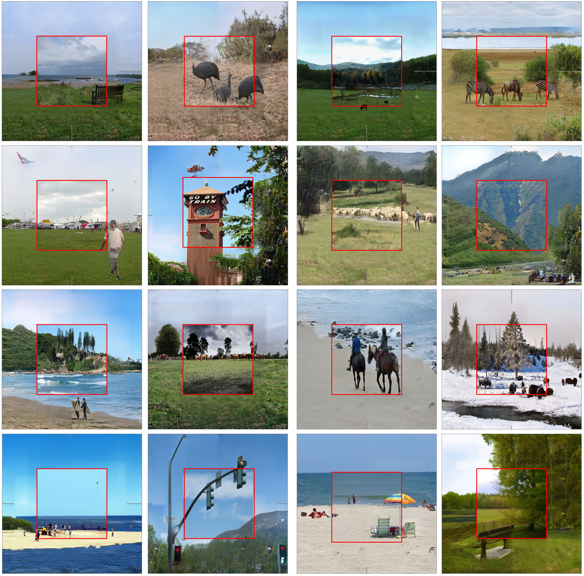
Given a scene patch at the center, our model can achieve scene extrapolation, i.e. generating beyond-the-border image content according to the semantic map guidance. A $512\times 512$ extrapolated images is generated by weighted combining synthesized $256\times 256$ patches at $4$ corners and $10$ other random locations. As shown in Fig. 9, our model generates visually plausible extrapolated images, showing the promise of our proposed framework for guided scene panorama generation.

Swapping Style Fig. 10 shows reference-guided style swapping on six distinctively different scenes. For the same segmentation mask, we generate multiple outputs using different reference images. Our approach can reasonably transfer styles among multiple scenes, including grassland, dessert, ocean view, ice land, etc. More results are included in the appendix.

5 Conclusion

We propose to address a challenging example-guided scene image synthesis task. To propagate information between structurally uncorrelated and semantically unaligned scenes, we propose an MSCA module that leverages decoupled cross-attention for adaptive correspondence modeling. With MSCA, we propose a unified model for joint global-local alignment and image synthesis. We further propose a patch-based self-supervision scheme that enables training. Experiments on the COCO-stuff dataset show significant improvements over the existing methods. Furthermore, our approach provides interpretability and can be extended to other content manipulation tasks.

References

(1) Martin Arjovsky, Soumith Chintala, and Léon Bottou. Wasserstein gan. arXiv preprint arXiv:1701.07875, 2017.
(2) Andrew Brock, Jeff Donahue, and Karen Simonyan. Large scale gan training for high fidelity natural image synthesis. arXiv preprint arXiv:1809.11096, 2018.
(3) Holger Caesar, Jasper Uijlings, and Vittorio Ferrari. Coco-stuff: Thing and stuff classes in context. In Proceedings of the IEEE Conference on Computer Vision and Pattern Recognition, pages 1209–1218, 2018.
(4) Huiwen Chang, Jingwan Lu, Fisher Yu, and Adam Finkelstein. Pairedcyclegan: Asymmetric style transfer for applying and removing makeup. In Proceedings of the IEEE Conference on Computer Vision and Pattern Recognition, pages 40–48, 2018.
(5) Qifeng Chen and Vladlen Koltun. Photographic image synthesis with cascaded refinement networks. In Proceedings of the IEEE International Conference on Computer Vision, pages 1511–1520, 2017.
(6) Yunpeng Chen, Yannis Kalantidis, Jianshu Li, Shuicheng Yan, and Jiashi Feng. Aˆ 2-nets: Double attention networks. In Advances in Neural Information Processing Systems, pages 352–361, 2018.
(7) Alexei A Efros and William T Freeman. Image quilting for texture synthesis and transfer. In Proceedings of the 28th annual conference on Computer graphics and interactive techniques, pages 341–346. ACM, 2001.
(8) Leon A Gatys, Alexander S Ecker, and Matthias Bethge. Image style transfer using convolutional neural networks. In Proceedings of the IEEE conference on computer vision and pattern recognition, pages 2414–2423, 2016.
(9) Leon A Gatys, Alexander S Ecker, and Matthias Bethge. Image style transfer using convolutional neural networks. In Proceedings of the IEEE conference on computer vision and pattern recognition, pages 2414–2423, 2016.
(10) Ian Goodfellow, Jean Pouget-Abadie, Mehdi Mirza, Bing Xu, David Warde-Farley, Sherjil Ozair, Aaron Courville, and Yoshua Bengio. Generative adversarial nets. In Advances in neural information processing systems, pages 2672–2680, 2014.
(11) Shuyang Gu, Congliang Chen, Jing Liao, and Lu Yuan. Arbitrary style transfer with deep feature reshuffle. In Proceedings of the IEEE Conference on Computer Vision and Pattern Recognition, pages 8222–8231, 2018.
(12) Aaron Hertzmann, Charles E Jacobs, Nuria Oliver, Brian Curless, and David H Salesin. Image analogies. In Proceedings of the 28th annual conference on Computer graphics and interactive techniques, pages 327–340. ACM, 2001.
(13) Martin Heusel, Hubert Ramsauer, Thomas Unterthiner, Bernhard Nessler, and Sepp Hochreiter. Gans trained by a two time-scale update rule converge to a local nash equilibrium. In Advances in Neural Information Processing Systems, pages 6626–6637, 2017.
(14) Jie Hu, Li Shen, and Gang Sun. Squeeze-and-excitation networks. In Proceedings of the IEEE conference on computer vision and pattern recognition, pages 7132–7141, 2018.
(15) Haozhi Huang, Hao Wang, Wenhan Luo, Lin Ma, Wenhao Jiang, Xiaolong Zhu, Zhifeng Li, and Wei Liu. Real-time neural style transfer for videos. In Proceedings of the IEEE Conference on Computer Vision and Pattern Recognition, pages 783–791, 2017.
(16) Xun Huang and Serge Belongie. Arbitrary style transfer in real-time with adaptive instance normalization. In Proceedings of the IEEE International Conference on Computer Vision, pages 1501–1510, 2017.
(17) Xun Huang, Ming-Yu Liu, Serge Belongie, and Jan Kautz. Multimodal unsupervised image-to-image translation. In Proceedings of the European Conference on Computer Vision (ECCV), pages 172–189, 2018.
(18) Xun Huang, Ming-Yu Liu, Serge Belongie, and Jan Kautz. Multimodal unsupervised image-to-image translation. In Proceedings of the European Conference on Computer Vision (ECCV), pages 172–189, 2018.
(19) Phillip Isola, Jun-Yan Zhu, Tinghui Zhou, and Alexei A Efros. Image-to-image translation with conditional adversarial networks. In Proceedings of the IEEE conference on computer vision and pattern recognition, pages 1125–1134, 2017.
(20) Max Jaderberg, Karen Simonyan, Andrew Zisserman, et al. Spatial transformer networks. In Advances in neural information processing systems, pages 2017–2025, 2015.
(21) Justin Johnson, Alexandre Alahi, and Li Fei-Fei. Perceptual losses for real-time style transfer and super-resolution. In European conference on computer vision, pages 694–711. Springer, 2016.
(22) Tero Karras, Timo Aila, Samuli Laine, and Jaakko Lehtinen. Progressive growing of gans for improved quality, stability, and variation. arXiv preprint arXiv:1710.10196, 2017.
(23) Tero Karras, Samuli Laine, and Timo Aila. A style-based generator architecture for generative adversarial networks. In Proceedings of the IEEE Conference on Computer Vision and Pattern Recognition, pages 4401–4410, 2019.
(24) Diederik P Kingma and Jimmy Ba. Adam: A method for stochastic optimization. arXiv preprint arXiv:1412.6980, 2014.
(25) Hsin-Ying Lee, Hung-Yu Tseng, Jia-Bin Huang, Maneesh Singh, and Ming-Hsuan Yang. Diverse image-to-image translation via disentangled representations. In Proceedings of the European Conference on Computer Vision (ECCV), pages 35–51, 2018.
(26) Jing Liao, Yuan Yao, Lu Yuan, Gang Hua, and Sing Bing Kang. Visual attribute transfer through deep image analogy. arXiv preprint arXiv:1705.01088, 2017.
(27) Jianxin Lin, Yingce Xia, Tao Qin, Zhibo Chen, and Tie-Yan Liu. Conditional image-to-image translation. In Proceedings of the IEEE Conference on Computer Vision and Pattern Recognition, pages 5524–5532, 2018.
(28) Ce Liu, Jenny Yuen, and Antonio Torralba. Sift flow: Dense correspondence across scenes and its applications. IEEE transactions on pattern analysis and machine intelligence, 33(5):978–994, 2010.
(29) Ming-Yu Liu, Thomas Breuel, and Jan Kautz. Unsupervised image-to-image translation networks. In Advances in neural information processing systems, pages 700–708, 2017.
(30) Ziwei Liu, Ping Luo, Xiaogang Wang, and Xiaoou Tang. Deep learning face attributes in the wild. In Proceedings of the IEEE international conference on computer vision, pages 3730–3738, 2015.
(31) Fujun Luan, Sylvain Paris, Eli Shechtman, and Kavita Bala. Deep photo style transfer. In Proceedings of the IEEE Conference on Computer Vision and Pattern Recognition, pages 4990–4998, 2017.
(32) Liqian Ma, Xu Jia, Stamatios Georgoulis, Tinne Tuytelaars, and Luc Van Gool. Exemplar guided unsupervised image-to-image translation with semantic consistency. arXiv preprint arXiv:1805.11145, 2018.
(33) Xudong Mao, Qing Li, Haoran Xie, Raymond YK Lau, Zhen Wang, and Stephen Paul Smolley. Least squares generative adversarial networks. In Proceedings of the IEEE International Conference on Computer Vision, pages 2794–2802, 2017.
(34) Mehdi Mirza and Simon Osindero. Conditional generative adversarial nets. arXiv preprint arXiv:1411.1784, 2014.
(35) Takeru Miyato, Toshiki Kataoka, Masanori Koyama, and Yuichi Yoshida. Spectral normalization for generative adversarial networks. arXiv preprint arXiv:1802.05957, 2018.
(36) Taesung Park, Ming-Yu Liu, Ting-Chun Wang, and Jun-Yan Zhu. Semantic image synthesis with spatially-adaptive normalization. In Proceedings of the IEEE Conference on Computer Vision and Pattern Recognition, 2019.
(37) Andreas Rössler, Davide Cozzolino, Luisa Verdoliva, Christian Riess, Justus Thies, and Matthias Nießner. Faceforensics: A large-scale video dataset for forgery detection in human faces. arXiv preprint arXiv:1803.09179, 2018.
(38) Tim Salimans, Ian Goodfellow, Wojciech Zaremba, Vicki Cheung, Alec Radford, and Xi Chen. Improved techniques for training gans. In Advances in neural information processing systems, pages 2234–2242, 2016.
(39) Aliaksandr Siarohin, Enver Sangineto, Stéphane Lathuilière, and Nicu Sebe. Deformable gans for pose-based human image generation. In Proceedings of the IEEE Conference on Computer Vision and Pattern Recognition, pages 3408–3416, 2018.
(40) Karen Simonyan and Andrew Zisserman. Very deep convolutional networks for large-scale image recognition. arXiv preprint arXiv:1409.1556, 2014.
(41) Miao Wang, Guo-Ye Yang, Ruilong Li, Run-Ze Liang, Song-Hai Zhang, Peter Hall, Shi-Min Hu, et al. Example-guided style consistent image synthesis from semantic labeling. arXiv preprint arXiv:1906.01314, 2019.
(42) Ting-Chun Wang, Ming-Yu Liu, Jun-Yan Zhu, Guilin Liu, Andrew Tao, Jan Kautz, and Bryan Catanzaro. Video-to-video synthesis. arXiv preprint arXiv:1808.06601, 2018.
(43) Ting-Chun Wang, Ming-Yu Liu, Jun-Yan Zhu, Andrew Tao, Jan Kautz, and Bryan Catanzaro. High-resolution image synthesis and semantic manipulation with conditional gans. In Proceedings of the IEEE conference on computer vision and pattern recognition, pages 8798–8807, 2018.
(44) Xiaolong Wang, Ross Girshick, Abhinav Gupta, and Kaiming He. Non-local neural networks. In Proceedings of the IEEE Conference on Computer Vision and Pattern Recognition, pages 7794–7803, 2018.
(45) Zhou Wang, Alan C Bovik, Hamid R Sheikh, Eero P Simoncelli, et al. Image quality assessment: from error visibility to structural similarity. IEEE transactions on image processing, 13(4):600–612, 2004.
(46) Jaejun Yoo, Youngjung Uh, Sanghyuk Chun, Byeongkyu Kang, and Jung-Woo Ha. Photorealistic style transfer via wavelet transforms. arXiv preprint arXiv:1903.09760, 2019.
(47) Fisher Yu, Wenqi Xian, Yingying Chen, Fangchen Liu, Mike Liao, Vashisht Madhavan, and Trevor Darrell. Bdd100k: A diverse driving video database with scalable annotation tooling. arXiv preprint arXiv:1805.04687, 2018.
(48) Han Zhang, Ian Goodfellow, Dimitris Metaxas, and Augustus Odena. Self-attention generative adversarial networks. arXiv preprint arXiv:1805.08318, 2018.
(49) Richard Zhang, Phillip Isola, Alexei A Efros, Eli Shechtman, and Oliver Wang. The unreasonable effectiveness of deep features as a perceptual metric. In Proceedings of the IEEE Conference on Computer Vision and Pattern Recognition, pages 586–595, 2018.
(50) Jun-Yan Zhu, Taesung Park, Phillip Isola, and Alexei A Efros. Unpaired image-to-image translation using cycle-consistent adversarial networks. In Proceedings of the IEEE international conference on computer vision, pages 2223–2232, 2017.

Appendix A The Synthesis Module

As shown in Fig. 11, our image synthesis module (the dash block on the right) takes the image features map $F^{(i)}_{x,1}$ and segmentation features map $F^{(i)}_{c,1}$ as inputs to output a new image $\hat{x}_{2\shortrightarrow 1}$ . Specifically, at each scale, a SPADE residue block spade with upsampling layer takes the concatenation of $F^{(i)}_{x,1}$ and $F^{(i)}_{c,1}$ as input to generate an upsampled feature map or image.

Figure 11: The details of the image synthesis module (the dash block on the right). The image synthesis module takes image features maps

F^{(i)}_{x,1}

and segmentation features maps

F^{(i)}_{c,1}

at all scale

i

as inputs to output a new image

\hat{x}_{2\shortrightarrow 1}

. Multiple SPADE residue blocks spade with upsampling layers are used to upsample the spatial resolutions.

Appendix B MSCA Pretraining

As shown in Fig. 12, an auxiliary feature decoder (the dash block on the right) is used to pretrain the feature extractors and the MSCA modules. Specifically, at each scale, the concatenation of $F^{(i)}_{x,1}$ and $F^{(i)}_{c,1}$ at each scale is fed into a $1\times 1$ convolutional layer to reconstruct the ground-truth VGG feature of $x_{1}$ at the corresponding scale. We weighted sum the L1 losses between predictions and ground-truth at each scales, then apply backpropagation to update weights of the whole model. We pretrain the model for $20$ epochs. Because of the light-weight design of the feature decoder, the pretraining step only takes around $12$ hours, and around $4$ % of the total training time.

Figure 12: The details of the auxiliary feature decoder for feature extractor and MSCA pretraining (dash block on the right). At each scale

i

, the image features map

F^{(i)}_{x,1}

and the segmentation features map

F^{(i)}_{c,1}

are concatenated and feed to a

1\times 1

convolution layer to predict the VGG-19 features map of

x_{1}

Appendix C Results of example_cvpr18; example_cvpr19

We provide additional results of conditional image-to-image translation (Conditional I2I) example_cvpr18 and style-guided synthesis example_cvpr19 in Fig. 13, column 9 and 10. To train the model of example_cvpr18, we resize images and semantic label maps to $64$ , the original resolution used in example_cvpr18. We test different learning rates and early stopping strategies to prevent the generator from model collapse. To implement example_cvpr19, we train the model of example_cvpr19 using our patch-based self-supervision. We test multiple learning rates and channel sizes of the generator. However, we could not achieves good results for example_cvpr18 and example_cvpr19. We believe the disentanglement strategy of example_cvpr18 is too challenging for the highly diversified COCO-stuff dataset. Meanwhile, input domain concatenation used in example_cvpr19 may not be sufficient to capture and fuse the style information for the more challenging scene image dataset. In addition, spatially-adaptive normalization spade might be required for example_cvpr19 to better utilize the captured style coding.

Appendix D More Style Swapping Results

We show style swapping results on $12$ diversified scenes in Fig. 14. As shown in the figure, our model can transfer styles to very different scene semantics and generate style consistent outputs given exemplar images.