Information recovery from pure state geometries in 3D
Abstract
It is a well-studied phenomenon in AdS3/CFT2 that pure states often appear ‘too thermal’ in the classical gravity limit, leading to a version of the information puzzle. One example is the case of a heavy scalar primary state, whose associated classical geometry is the BTZ black hole. Another example is provided by a heavy left-moving primary, which displays late time decay in chiral correlators.
In this paper we study a special class of pure state geometries which do not display such information loss. They describe heavy CFT states created by a collection of chiral operators at various positions on the complex plane. In the bulk, these take the form of multi-centered solutions from the backreaction of a collection of spinning particles, which we construct for circular distributions of particles. We compute the two-point function of probe operators in these backgrounds and show that information is retrieved.
We observe that the states for which our geometric picture is reliable are highly extended star-like objects in the bulk description. This may point to limitations of semiclassical microstate geometries for understanding the information puzzle and to the need for including quantum effects.
1 Introduction and summary
The question of how information is returned from evaporating black holes Hawking:1974sw in a unitary theory of quantum gravity continues to challenge standard notions of the horizon and the validity of effective field theory Mathur:2009hf; Almheiri:2012rt. For eternal black holes in Anti-de-Sitter (AdS) spacetimes, a simple manifestation of the information puzzle was pointed out in Maldacena:2001kr in the context of the AdS/CFT correspondence Maldacena:1997re. In this case, the black hole geometry gives a description of the thermofield double state, yet it is ‘too thermal’ to correctly capture the late-time behaviour of correlators in the thermofield double state. A related manifestation of information loss in the context of AdS3/CFT2 was investigated in Fitzpatrick:2016ive: the classical geometry associated to a heavy primary state is the BTZ black hole Banados:1992wn. This geometry is unreasonably thermal and leads to information-losing correlation functions which are not compatible with those of a pure state in a unitary CFT.
In this work we will simplify the setting even further by using two peculiarities of AdS3: the fact that the symmetry algebra splits in left- and right-moving parts and that in 2D CFTs there is a gap between particle-like and black-hole-like states set by the Virasoro central charge. This allows one to consider states in the CFT Hilbert space which are above the gap in the left-moving sector but below it in the right-moving sector. A primary state with these properties is naively described by an overrotating BTZ geometry with and : it formally describes a temperature for the left-movers . The boundary-to-boundary propagator for a particle with mass and spin in this geometry is, in the saddle point approximation, obtained by evaluating the particle worldline action proposed in Castro:2014tta. As we will show, the result is
| (1) |
In the late-time regime where and are large, this propagator decays exponentially for most values of the mass and spin, and in the chiral limit it is even identical to the propagator in a black hole with the same value of . This behaviour is again not compatible with a correlator probing a pure CFT state, leading to a left-moving version of the information puzzle. In Fitzpatrick:2016ive it was argued that the corrections which restore unitarity are non-perturbative effects in , whose bulk interpretation has so far remained mysterious.
In this paper we will construct a different class of geometries with and which do not display information loss. They represent non-primary states in the dual CFT which are created by acting on the vacuum with a collection of light left-moving primaries inserted at various points within the unit disk. As we shall see, these correspond in the bulk to multi-centered solutions from the backreaction of a collection of spinning particles. The particles move on geodesics and rotate at constant distance from the center of . Thus, in contrast to studies of the Vaidya metric Balasubramanian:2011ur; Balasubramanian:2012tu; Anous:2016kss they do not collapse on each other. Using the methods of Hulik:2016ifr; Hulik:2018dpl we construct the metric explicitly in the rotationally symmetric limit where the centers are distributed continuously on a circular shell. This geometry contains a throat region which is capped off inside the shell of matter. We analyze two-point functions in this background and show that they do not display the late-time decay characteristic of information loss. This suggests that for these pure CFT states, the semiclassical geometry does give an accurate description of the physics.
The idea of considering a shell of particles to mimic the black hole geometry has also been studied in a different context Lemos:2014eva; Lemos:2015xwa, Danielsson:2017riq; Danielsson:2017pvl and Crisostomo:2003xz. In Lemos:2014eva; Lemos:2015xwa the matter content of the shell is considered to be some fluid with pressure that stabilises the shell. In Crisostomo:2003xz using the junction conditions for the case of a collapsing shell it was derived that the shell gives rise to the BTZ geometry. The difference in our approach is that the particles are stabilised at fixed distance by angular momentum and that the consideration of the shell is only to make the problem analytically tractable. In principle one can have more complicated configurations with distinct particles placed at various distances from the center of .
We should also point out that our classical geometries representing pure states are similar to the microstate geometries studied within the fuzzball proposal for black holes Mathur:2005zp; Mathur:2009hf; Bena:2007kg; Bena:2015bea and that both approaches are qualitatively close in their description of information retrieval in the capped throat geometry (see Galliani:2016cai; Bombini:2017sge; Bena:2019azk for work on information retrieval in the fuzzball program). One point of difference with the microstate geometries picture, is that our multi-centered solutions are purely three-dimensional and as such somewhat more singular, having conical singularities corresponding to CFT vertex operator insertions. These singularities are expected to be resolved by quantum corrections in the UV completion of the theory. In the fuzzball paradigm on the other hand the microstate geometries are intrinsically higher dimensional, and feature the smoothening out of singularities11 1 Even so, conical singularities are still present in the fuzzball picture Lunin:2002bj. and the presence of nontrivial topology from the higher dimensional point of view. Inspiration for the current work also came from the black hole deconstruction proposal of Denef:2007yt, where microstates take the form of zero-entropy multi-centered D-brane configurations. Indeed, the particular D0-brane centers in a D6-anti-D6 background considered in Denef:2007yt lift to spinning particles in AdS3. In that setting, the backreaction on the non-gravitational fields in the 3D theory make the system hard to analyze Raeymaekers:2015sba; Raeymaekers:2017rdj.
Our results may also give some insight into the limit of validity of the description of microstates as semiclassical geometries. Indeed, we find that our information-preserving classical geometries are highly extended configurations in the bulk, spread out over distances larger than the scale set by the minimum size of the throat. If we extrapolate to the black hole regime, these would correspond to star-like configurations spread out over distances larger than the horizon, while microstate geometries are more tightly bound solutions whose size is about a Planck length greater than horizon Guo:2017jmi. This may point to limitations on the usefulness of microstate geometries for understanding the information puzzle (somewhat similar to those pointed out in Raju:2018xue), suggesting that typical microstates should rather be understood within the quantum regime. The importance of quantum effects has been stressed also within the fuzzball paradigm, see e.g. MathurFAQ.
The content of this paper is organised as follows. In section 2 we explain the general idea and introduce some necessary concepts. These are the eternal BTZ black hole, its AdS/CFT interpretation and the role of correlation functions as indicators for the loss or restoration of information. In section 3 we examine geometries with left temperature. We present how these chiral geometries fit into an ansatz involving a Liouville field, as well as their properties in terms of entropy and global geometry. We also examine the thermal behaviour of two-point functions, by evaluating the worldline action of spinning and spinless particles. In section 4 we construct a multi-centered solution with the same charges as the left-thermal geometry by considering a shell of particles. We derive the Einstein’s equations with spinning particle sources within the Liouville ansatz and examine the properties of the shell solution. In section 5 by examining geodesics we show how when the geodesic penetrates the shell information is restored. We present our conclusions in section 6.
2 Pure states and classical geometries
We start this section by recalling some aspects of the correspondence between CFT states and classical bulk geometries in AdS3/CFT2. We review how a heavy primary state appears unreasonably thermal in the classical gravity regime, leading to a version of the information puzzle. In this case quantum corrections are expected to significantly alter the classical geometrical picture. We then consider a different class of pure state geometries, which describe pure states created by a collection of primary operators inserted at widely separated points on the complex plane. We give a qualitative argument that such states lead to a geometry where the black hole throat is capped off and information should be returned. Though this argument is presently out of reach of computational verification, we will see in the following sections that a chiral version of the problem is in fact tractable, and demonstrate how information is preserved in a class of chiral pure states.
2.1 CFT vs geometry
Consider a correlation function of primary operators in a two-dimensional Euclidean CFT defined on the complex plane parametrized by :
| (2) |
The conformal Ward identities imply that the expectation value of the stress tensor22 2 To avoid carrying around factors of in what follows, our stress tensor is rescaled with respect to the standard normalization in the literature Belavin:1984vu: . Similarly, our in (4) is the rescaled conformal weight . In particular, of order one corresponds at large to a heavy operator with weight of order .
| (3) | |||||
| (4) |
and similarly for the antiholomorphic part . Upon conformally mapping to the cylinder and analytically continuing to Lorentzian signature, , we obtain the Lorentzian cylinder expectation value
| (5) |
and similarly for .
If the CFT under consideration has a holographic dual, meaning roughly that it has a large central charge and a sparse spectrum of low-lying states Heemskerk:2009pn, the above stress tensor expectation values translate into a classical AdS3 geometry due to Banados Banados:1998gg. The metric takes the form of an all-order Fefferman-Graham (FG) expansion,
| (6) |
Here and in the rest of the paper, we have set the AdS radius to one. The metric (6) solves the vacuum Einstein equations and satisfies asymptotic AdS3 boundary conditions; the boundary is a cylinder and the boundary stress tensor Balasubramanian:1999re computed from (6) is precisely . The coordinate system is valid near the boundary at . This geometry is expected to accurately capture the physics only if the two following approximations are valid:
- •
semiclassical approximation in the bulk, which corresponds to the limit of large central charge in the CFT.
- •
pure gravity approximation, where we neglect all fields in the bulk AdS3 besides gravity. In the dual CFT, this is justified if the contribution from the vacuum block in a specific channel dominates the amplitude, see Hartman:2013mia for details.
We will refer to this two-fold approximation as the ‘classical gravity approximation’. When valid, we can compute observables in the bulk by probing the metric (6). For example, the correlator in the presence of two additional insertions of a vertex operator , which is parametrically lighter so that it doesn’t backreact on the metric, is given by
| (7) |
Here, means the boundary-to-boundary propagator for the field dual to evaluated in the geometry (6). In the last equality we have indicated that in the saddle-point approximation, this propagator can be evaluated from the on-shell action of a worldline connecting the two boundary points. In what follows we will use bulk observables like (7) as a diagnostic to see whether the classical gravity approximation is justified, by comparing them with CFT expectations.
2.2 Two heavy scalar operators
Let us illustrate this classical gravity picture in the simple case where we consider the two-point function of a scalar operator of rescaled dimension ,
| (8) |
In this situation, fluctuations around the geometry (6) should probe the state created by . The stress tensor on the plane has second order poles in the origin and at infinity,
| (9) |
Plugging the latter into the Fefferman-Graham metric (6) yields a static, rotationally symmetric metric. Upon setting
| (10) |
and redefining the radial coordinate as
| (11) |
it reduces to the non-rotating BTZ metric Banados:1992wn
| (12) |
with mass parameter 33 3 Our dimensionless parameter is essentially the ADM mass in Planck units, namely .
| (13) |
In what follows it will be useful to use different coordinates where we go to conformal gauge on the constant time slices,
| (14) |
Then the vacuum Einstein equation implies that satisfies the Liouville equation:
| (15) |
One finds that the coordinates in (12) and (14) are related as
| (16) |
while the Liouville solution describing the BTZ metric (12) is
| (17) |
We can also build an (anti-)holomorphic ‘stress tensor’ from the Liouville field,
| (18) |
One easily checks that for the solutions (17) it takes the same form as the Euclidean boundary stress tensor
| (19) |
This formal equality of the Liouville stress tensor and the Euclidean boundary stress tensor holds generally in the class of metrics (14) Hulik:2016ifr. One should keep in mind that and were a priori quite different objects: the former characterizes the gravitational field in the interior of the Lorentzian bulk while the latter lives on the Euclideanized boundary plane. The relation (19) should therefore be seen as a boundary-bulk map44 4 In a similar vein, our bulk Liouville field is a priori different from the boundary Liouville field considered in Coussaert:1995zp; Martinec:1998wm which is associated to ; yet the relation (19) shows that they take the same form., which tells us for example how primary insertions on the boundary (second order poles in ) map to singularities in the gravitational field along worldline sources in the bulk. In section 3.2 below we will discuss a chiral version of the bulk-boundary map where we will make these statements more precise. This map will play an important role in the rest of the paper.
We can also compute observables in the state by probing the BTZ geometry (12). For example, by evaluating the worldline action of a particle of mass we obtain from (7) the saddle point approximation to the holographic two-point function of a light scalar primary operator of dimension (see Balasubramanian:1999zv or section 3.3 below for details of this calculation),
| (20) |
2.3 Particles vs. black hole microstates
We now describe in more detail the above classical gravity picture of the state in various regimes of and discuss its limitations. For above the black hole threshold, we will see that our classical geometry is not a very reliable guide to the physics and corrections are expected to be significant. This can be viewed as a manifestation of the breakdown of effective field theory near black holes Mathur:2005zp; Almheiri:2012rt in a simplified setting.
For the vacuum with (equivalently ), the geometry is global AdS3. For small enough in the range (equivalently ), the geometry is a conical defect at the centre of AdS and describes the backreaction of a spinless point particle Deser:1983nh. A three dimensional embedding of the spatial geometry is shown in Figure 1a.
While we do expect our classical gravity picture of this state to receive corrections near the conical singularity, observables computed in the naive geometry don’t show any obvious pathologies. A good test is to see whether probe correlation functions display any forbidden singularities. In Euclidean signature, the only singularities that arise in CFT correlators come from OPE limits, when some of the operators collide. Taking the result (20) for and continuing to Euclidean signature under which
| (21) |
we see that the correlator has only an allowed OPE singularity for , when the two probe vertex operators collide.
A quite different situation arises when we consider heavy states above the black hole threshold, in the regime or . The primary state is pure and is a black hole microstate, contributing to the microscopic entropy as counted by Cardy’s formula. The classical geometry (12) is the BTZ black hole metric with horizon at
| (22) |
In this case, one expects the corrections to the classical gravity picture to be significant for the following reasons.
First of all, the eternal black hole geometry does not satisfy the right boundary conditions to describe a state in the dual CFT on the boundary , since the full geometry extended beyond the coordinate singularity at in fact contains a second conformal boundary. This can be seen in the standard way by going to Kruskal-like coordinates, but we will discuss it here from the perspective of our Liouville parametrization (14). When , an important property of the conformal factor (17) is the periodicity in . The conformal boundary can be taken to correspond to the unit circle . The horizon then corresponds to ; this is the value for which the circle of constant reaches its smallest size. The geometry extends to smaller values of until one reaches the value where the conformal factor blows up; this can be shown to be a second conformal boundary. The Liouville solution (17) on the annulus describes the familiar Einstein-Rosen throat geometry of the eternal Schwarzschild black hole. Part of the throat geometry can be isometrically embedded in three dimensional Euclidean space and is shown in figure 1b.


Another reason for expecting significant corrections to the classical gravity approximation comes from looking at probe correlators. Considering again the 2-point function (20), for it becomes precisely the thermal two-point function of a CFT on the infinite real line Cardy:1986ie at temperature
| (23) |
which agrees with the Hawking temperature Hawking:1974sw of the BTZ black hole. At large timelike separations, taking , the correlator (20) tends to zero exponentially. This is a manifestation of the information puzzle Fitzpatrick:2016ive since, in a unitary CFT on the circle, the effects of the perturbation of the state at initial time should never get completely wiped out. This version of information loss is also closely related to the one discussed in Maldacena:2001kr in the context of the classical gravity description of the thermofield double state. A further sign of pathologies is the fact that the two-point function, when analytically continued to Euclidean signature using (21), has forbidden singularities at for .
As was emphasized in Fitzpatrick:2016ive, this overly thermal behaviour cannot arise in the exact four-point function of a unitary CFT on a compact space and with a finite amount of degrees of freedom. Therefore the corrections to our classical gravity approximation are guaranteed to arrest the late-time decay of the correlator and return information (or, in the Euclidean picture, to remove the forbidden singularities). From the CFT point of view, it was shown in Fitzpatrick:2014vua that the approximate thermal behaviour is due to the large- approximation to the vacuum conformal block. Furthermore it was argued in Fitzpatrick:2016ive that including corrections to the vacuum block which are nonperturbative in modifies the late-time decay at time scales of order . Although we presently lack an understanding of these quantum effects in terms of geometry, one would expect them to effectively cap off the Einstein-Rosen throat before the inner boundary at is reached. This constitutes a simple example where the semiclassical approximation breaks down in a region where one might naively expect it to be accurate.
Before going on to consider more general pure states it is also worth recalling Martinec:1998wm that the particle () and black hole () regimes of the classical metric (12) are distinguished by the type of Liouville solution describing the metric on spacelike slices. Any solution of the Liouville equation (15) gives rise to a 2D metric which can locally be transformed to the Poincaré disk metric
| (24) |
The map is however not single-valued in general and can have branch points. When encircling a branch point, undergoes a fractional linear transformation determined by a monodromy matrix in . The branch points are classified by the conjugacy class of into hyperbolic, parabolic or elliptic types.
In the particle regime of the solution (17) we have
| (25) |
Since the Liouville solution for this range of masses has elliptic monodromy.
On the other hand, above the black hole threshold we have:
| (26) |
Since , the Liouville solution in this class of the hyperbolic type. For the metrics with (global ) and the monodromy is trivial and of parabolic type respectively.
2.4 Classical caps for extended microstates?
In the previous section we argued that the naive classical geometry of a heavy primary should receive significant corrections. Before moving on to discuss non-primary states, we want to point out one further pathology of this classical description. The dual CFT has heavy primary operators inserted in and at . In the bulk, these map to sources in under the CFT-to-bulk map (19), yet these points ‘lie beyond the boundaries’ and are not part of the physical spacetime where (see Figure 2(a)). Therefore the points where energy is inserted in the CFT do not map to points in spacetime, indeed the black hole geometry does not have any localized sources. Hence the CFT region near the heavy vertex operator cannot be probed in the bulk. This is an additional reason to expect significant corrections to the classical picture.
So far we focused on primary states in the CFT but we can also consider non-primary heavy states. In the rest of the paper we want to look at pure states which are created by acting on the vacuum with a collection of primary operators inserted at various locations within the unit disk (see Figure 2(b)):
| (27) |
Using the OPE one sees that the resulting state is a highly complicated mix of primaries and descendants55 5 Recent work Datta:2019jeo has emphasized the importance of descendants as black hole microstates. (Figure 2(c)). We will take each of the primary vertex operators to satisfy so that each of the individual centers has a mass below the black hole threshold, yet such that the total mass is above the black hole threshold, . In terms of the Liouville field, such configurations would correspond to solutions with several elliptic singularities, such that the monodromy encircling all the singularities is of hyperbolic type66 6 It’s straightforward to verify that the product of elliptic elements can indeed be hyperbolic, see also e.g. Anderson. . From the above comments on the bulk-boundary map, one would expect that if these operators are inserted within the annulus roughly of size , they correspond to sources in points which are part of the bulk spacetime. These backreact classically on the geometry, producing a multi-centered solution with conical defect singularity at each center. In this situation, the Einstein-Rosen bridge is capped off through classical backreaction effects, and we should be able to study the return of information by doing classical computations in the bulk.
The above argument is of course rather sketchy and hard to make precise. For one, the static ansatz (14) will fail to describe such multi-centered solutions, since each of the centers will tend to fall toward the center of AdS3 due to the gravitational potential.77 7 It is amusing to see what happens when trying to describe multicentered solutions within the static ansatz Hulik:2016ifr: the equation for the lapse function is solvable only if the solution includes additional negative mass ‘spurious’ singularities (i.e. excess angles of multiples of ), which balance the attractive forces. Instead such bound states will be described by highly complicated time-dependent solutions. It might be possible to construct the solution in the Fefferman-Graham patch (6) provided one can determine the residues of the single poles in the boundary stress tensor (4). This amounts to knowledge of the CFT correlator; we hope to return to this approach in the future. We would also like to mention that similar ideas have been put forth in Jackson:2014nla, see also VerlindeCFTAdS.
In the rest of this paper we will instead consider the chiral version of the above idea, where we replace all the scalar CFT operators with purely chiral ones.
3 Left-chiral primaries and overspinning BTZ
In this section we will study the classical gravity geometry associated with a purely left-moving CFT primary, which is a BTZ geometry with angular momentum , in the ‘overspinning’ regime where . Though this geometry doesn’t have a horizon and is not a black hole, we will show that it nevertheless shares some features with a black hole. For one, the metric contains two conformal boundaries connected by a negative curvature throat. A second property is that a subset of correlation functions in this background behave ‘too thermally’ and display exponential late-time decay. For example the two-point function of chiral currents is the same as in a BTZ black hole with same temperature for the left-movers. These considerations lead to a chiral version of the information puzzle and the conclusion that quantum effects must significantly alter the classical geometry.
3.1 Overspinning BTZ metrics
We start by considering the classical geometry associated to the two-point function of a holomorphic primary current with left-moving dimension ,
| (28) |
where we take to be above the ‘chiral threshold’,
| (29) |
The stress tensor VEVs on the plane and the cylinder are
| (30) |
Plugging into the Fefferman-Graham metric (6) and redefining the radial coordinate we obtain an instance of the spinning BTZ metric with angular momentum :
| (31) |
The boundary stress tensor for the metric (31) is
| (32) |
and therefore (30) corresponds to
| (33) |
Note that we are in the overspinning regime where and where the geometry (31) does not have a horizon.
Since this regime of the BTZ metric is not often discussed, we first discuss some global aspects of the general overspinning BTZ metric. Without loss of generality we take
| (34) |
We restrict to so that is not below the global AdS3 vacuum value. The coefficient in (12), , is positive and finite in the range . The limit is a conformal boundary, while is a coordinate singularity where diverges. The metric components become regular there by passing to the coordinate
| (35) |
and one can show that the metric is regular in and can be extended to negative values of . Indeed, in Appendix A we describe the extended geometry, where is allowed to take values on the real line, as a quotient of global , and show that this quotient acts without fixed points, leading to a regular geometry. The overspinning regime in is therefore quite different from the one in higher dimensions where one encounters naked singularities. However the negative region does contains pathologies in the form of closed timelike curves, since the Killing vector generating the identification is timelike there.
A significant feature of this extended geometry is that when , a second conformal boundary is reached. This boundary is again a cylinder, yet now the periodic coordinate is a time coordinate while is a spatial coordinate. Despite these causal pathologies on the inner boundary, we can still ask the question if signals can be sent between the two boundaries. For this purpose we look for null geodesics which interpolate between the two conformal boundaries. The solution for , where is an affine parameter on the null geodesic, is
| (36) |
where and are the conserved charges due to and translation invariance respectively (to be identified with energy resp. angular momentum in the region). To interpolate between the to boundaries, the first term has to vanish so we need . In the overspinning regime (34) of interest only the
| (37) |
geodesics are real. It takes infinite affine parameter to go from one boundary to the other and consequently the boundaries are causally disconnected in this sense. It’s also interesting to look at the behaviour of , whose solution is
| (38) | |||||
| (39) |
The interpolating geodesics connect points with on each boundary with values shifted by .
Summarizing, the overspinning metric resembles a black hole in that the extended geometry contains a second conformal boundary. We will presently see that, as in the black hole regime, the two boundaries are connected by negative curvature throat geometry, though in this case it is embedded in the 3D geometry in a more subtle manner.
3.2 The Liouville throat
In this subsection we will see that the left-thermal geometries contain a submanifold with constant negative curvature which is conveniently described by a solution of Liouville theory Hulik:2016ifr; Hulik:2018dpl. For simplicity we will limit the discussion in this subsection to the regime of interest (33) where the right-movers are in the ground state, or , though it could easily be generalized to the regime where . It will be useful in what follows to keep left-moving stress tensor general for the moment and consider solutions with arbitrary . We will refer to this class of metrics as the chiral sector, since the right moving sector of the dual theory is in the ground state.
We first note that setting in the Fefferman-Graham metric (6) and changing to the coordinates , the metric in the chiral sector can be written as
| (40) |
In this form, time is fibered over a 2D base manifold. One now observes that the metric on the base, given by the last two terms in the above expression, has constant negative curvature. Therefore, if we make a coordinate transformation which brings this base metric in conformal gauge, i.e. such that
| (41) |
the field will satisfy Liouville’s equation (15). Summarizing, we have argued that the metrics in the chiral sector can be brought into the form
| (42) |
where satisfies Liouville’s equation (15). Without loss of generality, we can choose the coordinate such that the conformal boundary in (40) corresponds to . In Hulik:2016ifr, to which we refer for more details, it was shown that the AdS3 boundary conditions imply that the the holomorphic ‘stress tensor’ constructed out of the bulk Liouville field can be extended to the full complex plane so as to satisfy the reflection condition
| (43) |
The boundary stress tensor can be found to be
| (44) |
Analytically continuing to Euclidean signature and mapping the cylinder to the plane as in (21) with complex coordinate , we find that the holomorphic boundary stress tensor is formally identical to :
| (45) |
This should again be seen as a bulk-boundary map in the chiral sector, showing e.g. how CFT vertex operator insertions (producing second order poles in ) translate into sources for the bulk gravitational field. We will study these sources in more detail in the next Section.
Returning to the special case of the BTZ metric in the chiral sector, the transformation to the form (42) is accomplished by rewriting the metric (31) for in the fibered form
| (46) |
and transforming the base metric (i.e. the last two terms) to conformal gauge. Explicitly one finds
| (47) |
and the Liouville solution describing the chiral BTZ metric is
| (48) |
Also the holomorphic Liouville stress tensor is
| (49) |
As was the case for the static black hole, the overspinning geometry has a throat region described by a Liouville solution of hyperbolic type. The Liouville form (42) of the metric describes the fully extended solution including the region of negative , and the throat connects the outer boundary at or with the inner boundary at or . The narrowest point of the throat, where the horizon would be in the static black, is at or .
Another class of solutions within the chiral metrics (42), which will play an important role in what follows, are those where the Liouville field has an elliptic singularity. Here the base metric is as illustrated in figure 1a and has only one boundary and a conical singularity in the interior. We will show below that these solutions arise from the backreaction of a spinning particle source.
3.3 Late-time decay of two-point functions
A second feature that the overspinning metrics share with black holes is the late-time decay of correlation functions probing the state, at least for a subset of correlators.
Let us first recall some thermodynamics in the spinning BTZ black hole regime of the metric (31), when . One often formally defines the left- and right- moving temperatures
| (50) |
They are related to the Hawking temperature of the black hole as
| (51) |
and the entropies of the outer and inner horizons take a split form
| (52) |
Though the overspinning metric of interest (31) doesn’t have a horizon and is not in the black hole regime, we can from (50) formally associate a left-moving temperature to it. The aim in the rest of this section is to clarify what this statement means concretely in terms of physical observables in the theory.
3.3.1 Generic spacelike geodesics
To study the thermal behaviour from the bulk side we want to consider particle probes in the overspinning BTZ geometry that start and end at timelike separated points at the boundary, while in between capture the characteristics of the geometry by diving into the bulk. In Lorentzian signature, timelike geodesics don’t reach the boundary, and the desired geodesics are actually spacelike geodesics of infinite proper length Balasubramanian:2011ur.
Our starting point is the spinning BTZ metric (31) with the radial coordinate redefined to ,
| (53) |
We define
| (54) |
from which we infer the relations
| (55) |
For black holes are real, while in the overspinning regime they are complex and conjugate to each other.
We are interested in spacelike geodesics denoted by and parametrised by proper length such that
| (56) |
The BTZ metric has two killing vectors and from which get two conserved quantities
| (57) |
| (58) |
From (56), (57) and (58) we derive the corresponding differential equations
| (59) |
Solving these we find the spacelike geodesics
| (60) |
where we defined
| (61) |
Another class of solutions is similar to (60) but with replaced by . As we will see, in the black hole regime these solutions connect only spacelike separated points at the boundary. However they will be needed in the case of overspinning geometries. As long as are real, the above geodesics are real solutions both in the black hole and overspinning cases.
In the underspinning case (), are real and thus and blow up when the argument of arccoth becomes one. This can be regularized by considering complexified geodesics as in Balasubramanian:2012tu. However, in the overspinning case (), are complex and thus and remain finite. Thus no regularisation is needed and one can work with the geodesic equations as they are.
For AdS space:
We have , and
| (62) |
The and geodesics then simplify as
| (63) |
For the maximally overspinning case:
When , we have and
| (64) |
3.3.2 Evaluation of geodesic length
For spinless particles evaluating the worldline action amounts to finding the geodesic length
| (65) |
We calculate the proper length of geodesics starting and ending on the boundary at infinite . We regularise our computations by having the probe particle start and end at radial coordinate and take in the end. Also without loss of generality we will take . Thus we want to study geodesics between the points
| (66) |
After expanding in terms of and keeping terms up to order one we have
| (67) |
As explained in Balasubramanian:2011ur, this divergent quantity in the limit is to be renormalized by subtracting the divergent part in the global AdS geometry. After removing the regulator we then obtain
| (68) |
For this expression to make sense we must require
that the argument of the logarithm is greater than zero.
Our goal is to find the geodesic length as a function of . We have
| (69) |
which for the branch is
| (70) |
After solving the latter in terms of and expressing it in terms of we have
| (71) |
For the branch we find the above equation with the signs in reversed
| (72) |
Let us now use the above to express the argument of the logarithm in (68) as a function of . From (71) and (72) we have
| (73) |
where the plus sign is for the branch and the minus sign for the branch. Thus it is clear that in the black hole regime the above inequality is satisfied by the branch for timelike separated points, , and by the for spacelike separated points, .
In the overspinning case with the above equation becomes
| (74) |
In this case it is clear that once the sine becomes negative then we need to switch to the for the inequality to be satisfied. We also write the result for which will be useful later
| (75) |
3.3.3 Spin contribution to the two point function
Next we want to extend the above result for scalar particles to the computation of the probe two-point function of operators with spin. From the bulk point of view, in the saddle-point approximation this involves evaluating the worldline action for a spinning particle in the background. The motion of a point particle with intrinsic spin in general relativity is described by the Mathisson-Papapetrou-Dixon equations Mathisson:1937zz; Papapetrou:1951pa; Dixon:1970zza. In three dimensions, these equations can be derived from an action principle. This action was worked out in Castro:2014tta, and we will review it in more detail in section 4.1 below. For now it suffices to mention that in three dimensions, standard geodesics are still solutions of the equations of motion of the spinning particle. Therefore, to compute the spin dependence of the two-point function it suffices to evaluate the spin-dependent part of the action on the geodesics we constructed above. This spin-dependent part is given by
| (76) |
where is the spin of the particle and and are orthonormal vectors to the tangent vector ,
| (77) |
As shown in Castro:2014tta this spin term depends only on the boundary values of the normal vector and can be written as
| (78) |
where the vectors constitute a parallel transported frame normal to the geodesic and , . The spin term then measures how strongly the normal frame gets boosted with respect to the frame while being parallel transported from the starting point to the endpoint of the geodesic. For simplicity, we will explicitly compute the spin term (78) only in the black hole regime where and are real, and then analytically continue the result to the overspinning regime.
As argued in Castro:2014tta, the appropriate boundary condition to impose is to take and to be equal
| (79) |
In what follows we will take to take the form
| (80) |
This vector is not of unit length, however the formula (78) is scale invariant and so the normalization is not necessary. It can be shown that the choosing a different results in a constant factor in the two-point function which can be absorbed in the normalization of the operator.
The reference frame can be chosen arbitrarily in the initial point and then parallel transported to the final point. However, instead of finding a set of normal vectors in BTZ spacetime directly we use the fact that AdS and BTZ spaces are locally isomorphic via (180). Thus we can translate normal vectors from AdS to BTZ space.
In AdS space in lightcone Poincaré coordinates the parallel normal vectors are
| (81) | |||
| (82) |
where are the initial and final coordinates of the boundary interval and the parameter varies from in the initial point to in the final point. In particular the regularized initial and final values of are
| (83) | |||
| (84) | |||
| (85) | |||
| (86) |
To transform them into BTZ we need to substitute and for the endpoints. This maps the endpoints of the CFT interval to the interval at the boundary of BTZ spacetime with for the starting point and for the endpoint. Furthermore, and get transformed by the Jacobian
| (87) |
Now we can evaluate (78), which after simplifying the result and taking the exponential yields
| (88) |
Combining the results of the last two subsections we obtain the result for the probe two-point function of spinning operators in BTZ backgrounds anticipated in (1).
3.4 Further comments
We have argued in this section that the overspinning BTZ geometry shares some features with black holes, namely the presence of two boundaries and the thermal behaviour of certain correlators, leading to forbidden singularities in the Euclidean theory. As in the black hole case, this suggests a breakdown of the classical gravity approximation for the description of the pure state created by a heavy left-moving primary, and corrections are expected to be significant. Indeed, as in Fitzpatrick:2016ive, it can be argued that nonperturbative effects resolve the forbidden singularities in the correlator. In fact, the arguments presented to this effect in Fitzpatrick:2016ive also apply to the current chiral situation, since they rely on an analysis of Virasoro blocks which are holomorphically factorized.
Before moving on to analyze a class of pure states which have a reliable classical geometry with a capped throat which returns information, we end this section with some further comments and puzzles related to the overspinning BTZ geometry.
- •
As argued in Maldacena:2001kr, the extended BTZ black hole geometry can also be interpreted holographically as an (approximate) description of the thermofield double state Israel:1976ur. The properties of the overspinning BTZ geometry we discussed above suggest that it might allow a similar interpretation as a state in a product of two decoupled CFTs. In this case however the inner boundary has pathologies in the form of closed timelike boundary curves, which should be reflected in pathologies in the CFT living there. It’s an interesting open question whether a consistent double copy interpretation for the overspinning BTZ geometry is possible.
- •
Although, as we saw, the overspinning BTZ geometries behave thermally in some respects, the thermodynamics of these solutions is not so clear. They do not have a horizon and therefore no macroscopic entropy. To see this from the dual CFT side, we first note that we cannot apply Cardy’s formula
(89) since for the left-thermal solution is negative. As far as we are aware, there is no known universal expression for the degeneracy of chiral states of a holographic CFT in the limit of large dimension. However we can get some idea of the degeneracy from looking at examples. Consider the -th symmetric orbifold of a free seed CFT at large . The central charge of the orbifold CFT is . Purely chiral states which are in the right-moving ground state can come only from the untwisted sector (since the twisted sectors have non-vanishing right-moving zero-point energy) and can be seen to be in one-to-one correspondence with chiral states in the free seed theory. Their entropy is therefore
(90) and is down by a factor compared to the entropy carried by a BTZ black hole and counted by the Cardy formula.
4 Pure chiral states with a cap
In the previous section we discussed a form of the information paradox for chiral states: the classical geometry associated to a chiral primary state is ‘unreasonably thermal’ and is expected to receive significant corrections. In the rest of the paper, we will construct a class of chiral, non-primary, pure states which do not exhibit information loss in the classical gravity approximation. For this we will implement the chiral version of the idea outlined in section 2.4. The advantage of focusing on the chiral sector is that it is more tractable, since the bulk metric lies in the class of stationary metrics (42).
We want to study chiral, non-primary, pure states which are created by acting on the vacuum with a collection of primary chiral currents which are inserted at various locations within the unit disk,
| (91) |
where the rescaled weights satisfy so as to correspond to particle-like rather than black hole-like excitations. The classical bulk metric will be of the form (42) where the Liouville solution has elliptic singularities.
In the first part of this section, we will clarify the physical interpretation of these elliptic singularities in the bulk: they correspond to worldlines sources of spinning particles with equal mass and spin. In the second part, we will solve for the classical gravity metric for a circular array of operators in the limit where they form a continuous distribution. In the resulting metric, the Liouville throat region is capped off inside the matter shell. In the next section we will investigate whether correlation functions computed in this background display late-time decay.
4.1 Chiral current insertions from spinning particles
In this subsection we will show that insertions of chiral vertex operators with rescaled weights correspond to worldline sources of spinning particles in the bulk. The motion of a point particle with intrinsic spin in general relativity is described by the Mathisson-Papapetrou-Dixon equations Mathisson:1937zz; Papapetrou:1951pa; Dixon:1970zza. In three dimensions, these equations can be derived from an action principle, which can be used to derive the gravitational backreaction of spinning particles. This was worked out in Castro:2014tta, to which we refer for details.
The combined action for gravity and the spinning particles is (recall that we set )
| (92) | |||||
| (93) | |||||
| (94) |
Here, and are the mass and spin of the particle, describes the particle wordline and the covariant derivative on the worldline is defined as
| (95) |
The vectors are orthonormal to the velocity ,
| (96) |
Following Castro:2014tta, it is convenient to add Lagrange multiplier terms to the action which enforce these constraints.
The equations of motion from varying the total action with respect to the metric and the worldline variables are
| (97) | |||||
| (98) | |||||
| (99) |
Here, we defined reduced mass and spin parameters
| (100) |
and have chosen the worldline parameter to measure proper time, i.e. such that . The quantity is the spin tensor88 8 We normalized the -symbol such that .
| (101) |
Let us briefly comment on some important properties of these equations. First of all, the equation (99) for the particle trajectory is still solved by an ordinary geodesic : in three dimensions, spinning particles are still allowed to move on geodesics. There can also be non-geodesic solutions to (99), but we will not consider these in this work. It is also useful to note that, if the particle does move on a geodesic, the second term in (97) vanishes. A second remark concerns the fact that the spin-dependent source term (98) contains first derivatives of the delta function and is more singular than spinless particle sources. The inclusion of spin therefore leads to a more singular behaviour of the backreacted metric, as we will illustrate shortly.
Next we want to work out the equations (98) for the particular case of the backreaction of spinning particles in . We assume the metric ansatz (42)
| (102) |
and we want to backreact a particle on the trajectory at constant :
| (103) |
One easily shows that this trajectory is a geodesic, so that eq. (99) is satisfied, and that measures proper time. In global AdS3, the constant trajectories are curves which spiral around the center, see Figure 3.
Next we turn to the equations (98) for the backreacted geometry. One finds that, in order for the terms containing derivatives of delta functions to cancel, the gauge field strength should have a delta-function singularity99 9 Our delta-function is normalized such that , in particular we have .:
| (104) |
The remaining Einstein equations reduce to1010 10 Upon substituting (104) into Einstein’s equation, one obtains indeterminate terms which are contain factors like , which vanishes at the sources, multiplied by a singular factor from the square of the delta function. By writing the delta function as a limit of Gaussians one can show that these terms vanish. the Liouville equation with a source term
| (105) |
Near the source , the exponential term can be neglected for sufficiently small , and the stress tensor constructed from the Liouville field has a double pole
| (106) |
The equation (104) for the gauge potential can be solved in terms of to give, up to regular gauge transformations which can be reabsorbed in a redefinition of ,
| (107) |
The boundary stress tensor for such solutions, transformed to the Euclidean plane, is Hulik:2018dpl
| (108) |
From the second equality we see that ‘chiral’ particles, for which the mass and spin are equal:
| (109) |
do not excite the right-moving sector and produce a chiral metric in our earlier terminology. We will reσtrict our attention to such chiral particle sources in what follows. From the first equality in (108) and from (106) we see that inserting a chiral vertex operator in the CFT corresponds to adding a chiral particle source in the bulk.
The above comments on the backreaction of spinning particles provide a direct derivation in the metric formalism of properties which were derived in Hulik:2018dpl using Chern-Simons variables, where the coupling of spinning particles becomes particularly simple Castro:2014tta.
4.2 Solution for a shell of spinning particles
The discussion in the previous subsection generalizes in a straightforward manner to the inclusion of several spinning particle sources. We will presently derive the solution for a circular configuration of such particles in a continuum limit where they form a homogeneous shell.
We start from the Liouville equation (105) with sources from identical particles with mass and spin placed symmetrically on a circle of radius :
| (110) |
We take the continuum limit keeping fixed, in which the problem becomes rotationally symmetric and we can take to be a function of alone. The equation reduces to
| (111) |
where prime denotes a derivative with respect to , and is the mass per unit radial coordinate of the shell :
| (112) |
The solution to (111) will be of the matched form
| (113) |
with solutions of the Liouville equation without sources. The solution is the vacuum AdS3 solution. For the outside solution, we are interested in the case where it is above the black-hole-like threshold , so that is of the hyperbolic type and describes a chiral BTZ geometry. In what follows we will solve for the density of the shell in terms of the mass . Concretely, the inner and outer solutions are of the form:
| (114) |
The as yet undetermined positive parameter is introduced for the following reason: a priori the radial coordinates inside and outside of the shell are unrelated, and the shell could be at different values for the inside and outside radial coordinate. By adjusting the parameter we can assume that is continuous across the shell, which is located at both in the inside and outside coordinates.
Substituting (113) into (111) we obtain the equations
| (115) | |||||
| (116) |
These impose the continuity of across the shell and relate the jump in the radial derivative to the source density . Using the first equation to solve for we get
| (117) |
Here, we have chosen the appropriate branch for which is positive. The matching condition (116) reduces to
| (118) |
In these formulas, the shell radius should be taken to lie between the inner and outer boundaries of the throat geometry, i.e. in the range . One can show that, for fixed mass , is a positive, monotonically decreasing function of which interpolates between at the inner boundary and 0 at the outer boundary. Therefore for every shell radius in the range there is a unique value of the source density for which (111) is solved.
When embedded in 3D Euclidean space, the solutions look like a throat region glued to a cap along the shell of matter, see Figure 4. The deeper we make the throat, the greater is the required mass density of the shell. For fixed mass we can distinguish 3 cases, depending whether the geometry is capped off before, precisely at, or beyond the narrowest point of the throat. If we were describing, as in section 2, an actual black hole throat where the narrowest point is the horizon, the first case (Fig. 4(a)) would be a star-like configuration spread out over an area greater than the horizon, while the second case (Fig. 4(b)) would resemble1111 11 More precisely for a fuzzball the structure is argued Guo:2017jmi to appear just (i.e. about a Planck length) outside of the narrowest radius, though at the classical level it does not seem meaningful to make this distinction. a microstate geometry Mathur:2005zp. The last case (Fig. 4(c)), where the shell is placed beyond the narrowest point of the throat, does not have a stable counterpart in the black hole regime. We will argue below that in this case the classical gravity picture is unreliable and subject to significant corrections.
The Liouville stress tensor for the solution (114) is
| (119) |
Here, we have extended to the complex plane so as to satisfy the reflection condition (43). Due to the relation (45) this is also the expression for the stress tensor in the Euclidean CFT. It’s useful to rewrite it as
| (120) |
with
| (121) |
This form makes it clear that it is the stress tensor of a continuous distribution of vertex operators at and their images at . The fact that this results in an expression (119) which is only piecewise holomorphic is familiar from CFT studies of continuous vertex operator distributions Anous:2016kss. Note that by considering a rotationally symmetric configuration we were able to obtain an analytic solution, in particular it determined the accessory parameters and in (120). In less symmetric situations this would require solving a difficult monodromy problem Hulik:2016ifr.
To write down the full 3D metric (102) we also have to specify the one-form , which we can read off from (107) with :
| (122) | |||||
Using (116) we note that the gauge field (and hence the metric) is not continuous across the shell but jumps by a large gauge transformation:
| (123) |
Such a jump in the metric components does not occur in the more familiar case of thin shells of non-spinning matter Israel:1966rt, and is a consequence of the more-singular-than-usual source term from the spin part of the action (98).
In what follows we would also like to display the above shell solution in BTZ coordinates. In the outside part we can make the coordinate transformation (47). On the inside we make the transformation
| (124) |
where is a parameter similar to , to be tuned such that the radial coordinates properly match up at the shell. From the above discussion we know that this requires that the base metric is continuous across the shell (rather than the full 3D metric), which leads to
| (125) |
where is the location of the shell in BTZ coordinates. Solving for gives
| (126) |
In conclusion, in BTZ coordinates our shell geometry takes the form
| (127) |
where the inner metric applies to and the outer one to .
5 Two-point function in shell background
In this section we compute the boundary-to-boundary propagator in the shell background (127) and investigate its late-time behaviour. As before we work in the saddle-point approximation where we have to evaluate the worldline action of boundary-to-boundary geodesics. This leads to a straightforward qualitative picture: as long as the geodesic lies completely outside of the shell the correlator behaves thermally, while once it starts penetrating the shell the behaviour will start resembling more and more the periodic answer in global AdS.
Despite being conceptually straightforward, the details of the calculation reveal interesting subtleties which are due to the fact that several geodesics can connect the same endpoints in the presence of the shell. As we will see, these lead to ‘swallow-tail’ phenomena and different geodesics exchanging dominance in the correlator. These phenomena are more pronounced as the shell is placed deeper in the throat region. Similar features were observed in other thin-shell computations such as Albash:2010mv; Balasubramanian:2012tu.
One important property that can be derived almost without computation is the following: when the shell radius is below the value where the throat geometry is at its narrowest (i.e. case (c) in Figure 4), the geodesics never penetrate the shell and the correlator will still decay at late times. Indeed, it can be seen from (60, 61) that none of the geodesics penetrates deeper into the bulk than
| (128) |
which is reached by geodesics with . We will comment more on this result in the Discussion.
5.1 Simplifying assumptions
As we saw in the previous section, the presence of spinning matter on the shell results in jumps in the fiber (123), which makes the problem of matching geodesics across the shell nontrivial. Fortunately however, as we shall presently argue, symmetry arguments can be used to reduce the problem to a computation in the 2D base geometry in (127), where the metric is continuous. A first simplification we will make is to restrict our attention here to the boundary-to-boundary propagator of a scalar particle with ; recall from (1) that this correlator displays late-time decay in the overspinning BTZ background. Secondly, since the shell is comprised of particles with (or, in the CFT language, the inserted vertex operators are chiral), the -dependence of the two-point function should be the same as in the global AdS3 background, namely the oscillating factor
| (129) |
It is therefore the dependence on the separation, for large , which decides whether the correlator decays at late times or not. To extract this dependence, we may just as well restrict to the subset of geodesics which have a fixed value of . In what follows, we will restrict attention to
| (130) |
The correlator for general can the be obtained by multiplying our result with
| (131) |
From our expressions for the geodesics in the BTZ geometry, we find (70) that, both in the global AdS3 and in the overspinning geometries, the geodesics with are the ones with equal energy and angular momentum,
| (132) |
The geodesics with are also the ones which have in the shell geometry, for the following reason. Let’s fix and first consider a shell with sufficiently small such that the geodesic does not penetrate it; it lies completely in the outer geometry and hence has . Now let’s move the shell outward until it crosses the geodesic; as we have argued this operation should not change the -dependence of the two-point function which is still (129), and therefore we must still have .
Now we observe that the geodesics with have the property that they live entirely in the two-dimensional base geometry, as the pullback of the first term in the outside metric (127) vanishes:
| (133) |
and similarly on the inside of the shell (note that the shell preserves translation invariance and therefore and are conserved also in the shell background). It is therefore the two-dimensional throat geometry which controls the late-time behaviour of the correlator, and we can reduce the problem to that of computing geodesic lengths in this 2D geometry.
5.2 Geodesics in the throat
In view of the above considerations, we first study general geodesics on the Euclidean two-dimensional base manifold with coordinates , and with metric
| (134) |
This space has a Killing vector which results in the conserved quantity given by
| (135) |
Parametrizing the geodesics by their proper length we have which results in the equation
| (136) |
From (135) and (136) we find three branches of geodesics: one branch with in the radial geodesic and two branches with . The latter will be needed to study geodesics that cross the shell, so with some foresight we include them here. For the branch we have
| (137) |
where .
For the two branches we have
| (138) |
We observe that the branch is valid for , while the branches are valid for . The branch involves geodesics that start and end at the same boundary at for . However, the branches extend from one boundary for to the other boundary for . In the case of the shell though this picture breaks down as the geometry caps off and there is only one boundary.
For the moment, we are not yet considering the presence of the shell and we move forward by making use of the branch. Also the solutions that differ by an overall sign through are related by . Again these solutions seem trivial at this point but they will play a significant role when we examine the shell.
For a geodesic starting from the boundary with we have
| (139) |
Thus,
| (140) |
Similarly
| (141) |
Solving the latter for and substituting back in (140), after renormalizing as in Section 3.3.2 and letting , we get
| (142) |
This expression decays exponentially for large as expected for the thermal solution. As a check, we see that it indeed matches the three dimensional computation (73) for . In order to have timelike separated endpoints at the boundary we need which requires for the argument of the logarithm to be positive.
For the AdS case, where , the hyperbolic sine turns into a sine and the behaviour becomes oscillatory, as expected for pure states.
| (143) |
Once again it matches the three dimensional result (75) for . Again we need for timelike separate points at the boundary. The choice of depends on the sign of sine. For example we have for and for . Thus even though the sine has period in terms of , the overall proper length has period .
5.3 Geodesics in the presence of the shell
We now look at geodesics with endpoints on the boundary in the presence of the shell placed at radius . For the metric outside and inside of the shell we respectively have
| (144) |
where was given in (126).
Not all geodesics will cross the shell: for small enough endpoint separation the geodesic will lie completely outside of the shell. With increasing the geodesics reach deeper into the bulk and eventually approach a minimum radius less than . More precisely, the minimum radius a geodesic reaches can be read off from (137),
| (145) |
which because of (140) and (142) gives
| (146) |
As already mentioned, for the geodesics never penetrate the shell and the geometry behaves as a left-thermal one. For the geodesic goes through the shell at given by
| (147) |
Furthermore, the geodesic that touches the shell has charge
| (148) |
We have that which means that it is the branch of geodesics that initially crosses the shell.
5.4 Shell 2-point function
We now construct the geodesics crossing the shell, pictured schematically in Figure 5. We denote the parameter values where the geodesic enters and exits the shell by and respectively. Thus the presence of the shell splits the geodesic into three segments: 1) segment “I” is for parameters between and before the geodesic crosses the shell, 2) segment “II” is for parameters between and when the geodesic is inside the shell and 3) segment “III” is for parameters between and when the geodesic comes out of the shell.
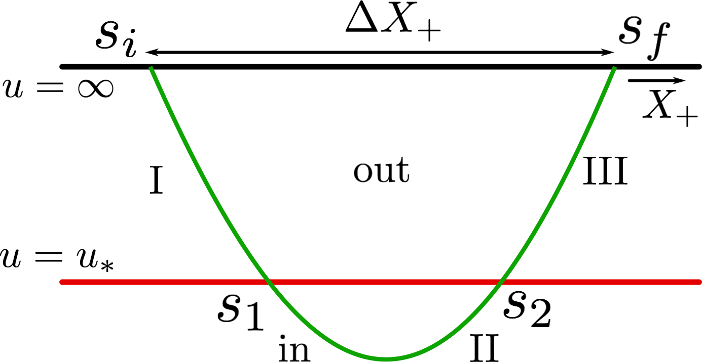
Since the presence of the shell preserves translation invariance, the associated conserved charge should be constant also in the presence of the shell, so that
| (149) |
As in Balasubramanian:2011ur this could be rewritten as a form of Snell’s law determining the refraction of geodesics when crossing the shell.
When all the segments of the geodesic are given by the branch and we have
| (150) |
For we have to use the branch but only in the segments of the geodesic outside the shell. Within the shell we always have and thus it is the branch that should be used. Furthermore, since we want the geodesic to start and end at the same boundary at , for sections and we should choose branches with different signs. Overall we have
| (151) |
and
| (152) |
For both cases without loss of generality we can choose the origin of such that . Regarding the sign coefficients, since outside the shell we should match the geodesics of a left-thermal geometry we choose . Inside the shell we keep the parameter , and we consider both signs similarly to pure AdS3.
Then, for each choice of , we overall we have ten parameters , which are fixed by the following ten boundary conditions and continuity equations.
The boundary conditions are
| (153) |
and the continuity equations are
| (154) |
Upon imposing these conditions we eventually find the geodesic length, renormalized as before in Section 3.3.2, for
| (155) |
and for
| (156) |
In the above expressions the first term is the result (142) for the left-thermal geometry, the second term subtracts out the length of the segment where in the left-thermal geometry, and the last term adds the length of the segment with in the AdS3 geometry. One can check that in the infinite shell limit we have
| (157) |
For the boundary separation of the endpoints we obtain
| (158) |
where is a integer and
| (159) |
Unlike in the geometry without shell, it is not possible to invert the dependence of on to find an analytic expression1212 12 It is possible to invert the dependence of on , by solving a cubic equation, and obtain , though the result is not very enlightening. for . In what follows we will rather parametrically plot in terms of using as a parameter. Before embarking into that, let us make here a few more analytical remarks.
Before crossing the shell the behaviour is that of a left thermal geometry and we have . At the geodesic touches the shell. At this point we have
| (160) |
However, (158) is defined only for . Thus after crossing the shell, as it can be seen from (158) and (159) we are confined to Within this range we see that (155) and (156) are well behaved finite functions. A possible pathological point seems to be for , but after carefully considering the limit we get
| (161) |
which is finite for . This point is a maximum for .
For we have the minimum for which is
| (162) |
The fact that the value of is bounded from below is already a sign of restoration of information. For the value of at this point we have for
| (163) |
and for
| (164) |
Overall taking into account the change in sign we have four different . Whether we use or depends on the value of the charge . Besides that we will parametrically plot as a function of for all possible signs and for all shifts. The actual contribution to will come from whichever term is more dominant for a specific value of .
5.5 Specific Examples
By setting specific values for the mass and radius of the shell we plot in fig.6 the logarithm of the two-point function as a function of . The different colours represent different branches of geodesics, see fig.7 for a colour legend. The leading saddle point approximation to the two-point function is obtained by selecting the branch with the highest value of for a given . We will see that these terms provide a suggestive picture about the shape of the geodesic and how much it penetrates the shell as we increase (fig.12).
Thermal and non-thermal behaviour:
Let us first discuss how the thermal behaviour of the two-point function is resolved in the shell geometry. For small values of the two-point function behaves as in the left-thermal geometry and is denoted with the gray line. At some point this thermal branch is crossed by one of the non-thermal branches. Beyond that point we observe oscillatory behaviour instead of the exponential decay in the left-thermal solution (dotted grey line).
Furthermore, for fixed shell mass, as we increase the radius of the shell, and bigger part of the geometry is AdS3, the crossing point and the maximum of are shifted higher as can be seen by comparing the plots fig.6, fig.8 and fig.9. In other words as we increase the radius of the shell, the behaviour of the geodesic length becomes more and more similar to what we would get in the case of pure AdS3 spacetime.
Cusps:
In the plots we observe several cusps or ‘swallow-tail’ phenomena (areas C1, C2, C3 in fig.6). While the geodesic length changes continuously as we change by moving along the coloured segments, the dominant contribution is discontinuous as we vary . However the total two-point function should be continuous. We believe this discrepancy is due to the saddle point approximation we adopted by studying geodesics. This effect has been observed elsewhere in literature both in the study of holographic thermalizationBalasubramanian:2011ur as well as in entanglement entropy Albash:2010mv.
We have two kinds of cusps in our plots. The first kind (C1 in fig.6) involves also the thermal branch which crosses over the non-thermal branches. A close up view is in fig.10. Although the geodesic touches the shell where the green and dashed lines meet, the contribution from geodesics entering the shell dominates already from an earlier value . This point is where red and gray lines intersect. As it can be seen from the plot the red branch is more dominant than the green one. Specifically at this cusp, due to the presence of the thermal branch, the dominant contribution is continuous. The second kind (C2) is depicted in fig.11. As we increase we move along the black line but the dominant branch jumps to the red line before the black line ends and overpassing the green line. A similar cusp, but with opposite orientation occurs when passing from the blue to the brown line, while overpassing the orange one (C3). As we will see in the next paragraph, this second kind of cusp involves transitioning from usual geodesics to geodesics with crossed external legs.
Behaviour of the non-thermal branches:
Let us now describe how the geodesic behaves (fig.12) as we move along the dominant part of the non-thermal branches of fig.6. At the cusps we also describe the behaviour at the non-dominant green and orange branches to present more accurately how the geodesic changes continuously and which shapes of geodesics are responsible for the discontinuity of the leading contribution at the cusp.
We start from the tip of the green line, which is the point the geodesic touches the shell (fig.12a) at , and . The geodesic goes deeper into the shell as we move along the green line and decreases (fig.12b). Then we reach the end of the green line, when , at the point where it meets the red line. The relevant geodesic is depicted by fig.12c. As we move along the red line the geodesic goes deeper into the shell (fig.12d), until we reach the minimum of where and (fig.12e). This brings us to the end of the red line.
Then the geodesic starts penetrating the shell less and less (blue line and fig.12f). We observe that after the point where , the legs of the geodesic for and appear to have been reversed, but that’s only because we are looking at the geodesic upside down. Then we reach the end of the blue line where it meets with the orange one at (fig.12g). Afterwards we reach the end of the orange line where it meets with the brown one at and . At this point the geodesic touches again the shell (fig.12h) as we have made a full angle on the shell.
However, there is still a that remains in order to reach at the on the boundary. To continue beyond this point one naively might expect that the geodesic exits the shell. That’s not what happens as the thermal branch at this point has decayed a lot and is far from being dominant. Instead this extra distance is covered by the branch with (brown line and ) and the external legs of the geodesic cross as seen in fig.12i. As we move towards the value we pass to the pink line () and the crossing point is moved closer to the boundary as seen in fig.12j. When we reach the crossing point has moved all the way to the boundary (fig.12k). This is the point where purple and pink lines meet in fig.6. The purple line represents another branch with but with .
As we keep increasing , the crossing point starts moving again towards the shell (purple and black lines and figures 12l and 12m respectively), until we reach the end of the black line, where it meets the green one and the geodesic touches the shell once more. At this point we have and . Then the legs of the geodesic stop crossing and the cycle starts again from the beginning.
6 Discussion and outlook
In this paper we examined the Lorentzian classical gravity geometries associated, à la Banados Banados:1998gg, to left-moving pure states in the dual CFT. To test the validity of the classical geometric picture, we compared the behaviour of the boundary-to-boundary two-point function evaluated in these geometries with CFT expectations.
For heavy primary states, we found that the geometry behaves as unreasonably thermal, leading to a chiral version of the information puzzle. One can argue, as in Fitzpatrick:2016ive, that nonperturbative effects should restore information.
We then studied a class of heavy, non-primary, pure states which are created by a dispersed collection of chiral vertex operators. The corresponding bulk geometry is a multi-centered solution with spinning particle sources, which is determined by a solution of classical Liouville theory with elliptic singularities. We constructed the metric in the rotationally symmetric case of a circular shell of particles. It contains a throat geometry which is capped off by the shell.
We then analyzed the probe two-point function in this background, whose late-time behaviour is governed by the capped throat geometry. When the shell is inserted before reaching the narrowest point of the throat (Fig. 4(a)), we found that information is returned when the relevant geodesics start exploring the geometry of the cap. However, when the shell is inserted beyond the narrowest point of the throat (Fig. 4(a)), the two-point function still decays. In the latter case, the classical geometry is not a reliable guide to the physics and finite corrections need to be considered to understand information recovery.
From these considerations we conclude that the states for which the semiclassical picture gives a reliable guide to information restoration are, from the bulk point of view, loosely bound states which are spread out over a distance larger than the scale set by the narrowest size of the throat. The states we considered in this work do not carry the quantum numbers of an actual black hole, being above the treshold only on the left-moving side of the CFT. Though we have not shown that it is valid to do so, if we extrapolate our findings to the black hole regime, the geometries for which we found information to be returned are star-like states spread out over super-horizon distances. As we discussed in Section 4.2, microstate geometries rather resemble the situation where the matter shell is just outside of the narrowest point of the throat as in Figure 4(b). In this case the geodesic grazes the shell without penetrating it and therefore we are at the limit where we can get an understanding of information recovery from the classical picture. This may point to limitations of the use of microstate geometries for understanding the return of information (somewhat similar to those raised in Raju:2018xue), suggesting that typical microstates should rather be understood within the quantum regime. The importance of quantum effects within the fuzzball paradigm has been stressed in e.g. MathurFAQ.
One possible caveat in the above is that some of the observed behaviour might be due the highly symmetric continuous distribution of particles operators we considered. This led to competing geodesics and swallow-tail phenomena which are especially significant when the shell is close to the narrowest point of the throat, making a complete analysis difficult in that case. It would therefore be interesting to get a handle on the less symmetric situation with discrete centers.
In continuing along the lines of the present work there are various open problems which we leave for the future. Specifically we would like to address the following:
- •
The most important issue to address is the generalisation of the constructions in the present work for spinning BTZ geometries with both sectors above the extremality bound. This would lead to the construction of classical microstates for non-extremal black holes within three-dimensional gravity.
- •
While the focus of this paper was on the bulk, it would be interesting to see how our results are reproduced by computations in the dual CFT at large . For two-point functions in the Vaidya geometry such an analysis was performed in Anous:2016kss. It would be particularly interesting to see how the CFT reproduces the various saddle points exchanging dominance; most likely this would come from a saddle point analysis of the integral that results from summing up contributions of the vacuum block from all points of the shell, as discussed in Anous:2017tza.
- •
As we mentioned above it would be interesting to explore less symmetric microstates consisting of several distinct particles in the bulk. An exact solution to such a problem is at the moment out of technical reach. However we believe one can gain some ground in this direction by using perturbative methods.
- •
As promoted in Castro:2018srf, there is an alternative method for evaluating the two-point function using Wilson lines. This method uses Chern-Simons variables which are more suitable for treating spinning probe particles. It should be interesting to perform the analysis of the shell solution using this alternative method and confirm the results presented here.
Appendix A Left-thermal geometries as quotients of global
To get more insight into the global properties of the overspinning BTZ metrics, it is useful to describe them as quotients of global AdS3. This is most conveniently achieved by embedding the geometry into a flat 4-dimensional ambient space with metric of signature :
| (165) |
Global is embedded as the submanifold
| (166) |
The embedding coordinates can be arranged in an group element
| (167) |
in terms of which the metric reads
| (168) |
We define the left-moving temperature and the parameter as
| (169) |
These are real and positive for the overspinning BTZ metrics of interest. The appropriate group element these metrics reads
| (170) |
where is given by
| (171) |
We note that is real and finite for all ; therefore the region (with CTCs) is part of the geometry. Substituting (170) into (168) we indeed find (31), where
| (172) |
Explicitly, the embedding coordinates are given by
| (173) |
We can now show that the overspinning geometries are regular quotients of AdS3. The periodic identification implies at the level of the group element
| (174) |
where and are constant matrices of boost resp. rotation type:
| (175) |
By inspecting the action on the embedding coordinates, one finds that the only fixed point is , which lies outside the AdS submanifold (166). We conclude that the overspinning BTZ geometry arises as a quotient of global AdS which acts without fixed points and is therefore completely smooth. The identification group is generated by where is the infinitesimal Killing vector. In terms of the Killing vectors of global AdS
| (176) |
where indices are lowered with , can be written as
| (177) |
To find out where this quotient belongs in the general classification of Banados:1992gq, we write the generator as and consider the eigenvalues of . These are purely imaginary and given by
| (178) |
and therefore the quotient giving rise to overspinning BTZ is of type in the classification of Banados:1992gq App. A (rather than of type as was conjectured there).
In conclusion, in contrast to the situation higher dimensions, the overspinning BTZ geometry is a smooth manifold. The metric does contain other pathologies in the form of closed timelike curves in the region where the generating Killing vector is timelike.
Appendix B Coordinate transformation between AdS and BTZ
AdS and BTZ spaces are locally isomorphic. Let us briefly recapitulate the coordinate transformation constituting this relation. In the Poincare coordinates the metric of AdS space reads
| (179) |
where we have set and defined . The desired coordinate transformation is
| (180) |
where are the left and right temperatures and are the boundary BTZ coordinates. Applying this coordinate transformation to the metric yields the BTZ metric.
Acknowledgements.
We would like to thank Dionysios Anninos, Tarek Anous, Roberto Oliveri, Iosif Bena and Nicholas Warner for valuable discussions and correspondence. This project was supported by the Grant Agency of the Czech Republic under the grant 17-22899S and by ESIF and MEYS (Project CoGraDS - CZ.02.1.01/0.0/0.0/15 003/0000437). O.V. would also like to thank the Erwin Schrodinger International Institute for Mathematics and Physics, for hospitality while this work was in progress.References
- (1) S. W. Hawking, “Particle Creation by Black Holes,” Commun. Math. Phys. 43 (1975) 199–220. [,167(1975)].
- (2) S. D. Mathur, “The Information paradox: A Pedagogical introduction,” Class. Quant. Grav. 26 (2009) 224001, arXiv:0909.1038 [hep-th].
- (3) A. Almheiri, D. Marolf, J. Polchinski, and J. Sully, “Black Holes: Complementarity or Firewalls?,” JHEP 02 (2013) 062, arXiv:1207.3123 [hep-th].
- (4) J. M. Maldacena, “Eternal black holes in anti-de Sitter,” JHEP 04 (2003) 021, arXiv:hep-th/0106112 [hep-th].
- (5) J. M. Maldacena, “The Large N limit of superconformal field theories and supergravity,” Int. J. Theor. Phys. 38 (1999) 1113–1133, arXiv:hep-th/9711200 [hep-th]. [Adv. Theor. Math. Phys.2,231(1998)].
- (6) A. L. Fitzpatrick, J. Kaplan, D. Li, and J. Wang, “On information loss in AdS3/CFT2,” JHEP 05 (2016) 109, arXiv:1603.08925 [hep-th].
- (7) M. Banados, C. Teitelboim, and J. Zanelli, “The Black hole in three-dimensional space-time,” Phys. Rev. Lett. 69 (1992) 1849–1851, arXiv:hep-th/9204099 [hep-th].
- (8) A. Castro, S. Detournay, N. Iqbal, and E. Perlmutter, “Holographic entanglement entropy and gravitational anomalies,” JHEP 07 (2014) 114, arXiv:1405.2792 [hep-th].
- (9) V. Balasubramanian, A. Bernamonti, J. de Boer, N. Copland, B. Craps, E. Keski-Vakkuri, B. Muller, A. Schafer, M. Shigemori, and W. Staessens, “Holographic Thermalization,” Phys. Rev. D84 (2011) 026010, arXiv:1103.2683 [hep-th].
- (10) V. Balasubramanian, A. Bernamonti, B. Craps, V. Keränen, E. Keski-Vakkuri, B. Müller, L. Thorlacius, and J. Vanhoof, “Thermalization of the spectral function in strongly coupled two dimensional conformal field theories,” JHEP 04 (2013) 069, arXiv:1212.6066 [hep-th].
- (11) T. Anous, T. Hartman, A. Rovai, and J. Sonner, “Black Hole Collapse in the 1/c Expansion,” JHEP 07 (2016) 123, arXiv:1603.04856 [hep-th].
- (12) O. Hulík, T. Procházka, and J. Raeymaekers, “Multi-centered AdS3 solutions from Virasoro conformal blocks,” JHEP 03 (2017) 129, arXiv:1612.03879 [hep-th].
- (13) O. Hulík, J. Raeymaekers, and O. Vasilakis, “Multi-centered higher spin solutions from conformal blocks,” JHEP 11 (2018) 101, arXiv:1809.01387 [hep-th].
- (14) J. P. S. Lemos and G. M. Quinta, “Entropy of thin shells in a (2+1)-dimensional asymptotically AdS spacetime and the BTZ black hole limit,” Phys. Rev. D89 no. 8, (2014) 084051, arXiv:1403.0579 [gr-qc].
- (15) J. P. S. Lemos, F. J. Lopes, and M. Minamitsuji, “Rotating thin shells in (2 + 1)-dimensional asymptotically AdS spacetimes: Mechanical properties, machian effects, and energy conditions,” Int. J. Mod. Phys. D24 no. 09, (2015) 1542022, arXiv:1506.05454 [gr-qc].
- (16) U. H. Danielsson, G. Dibitetto, and S. Giri, “Black holes as bubbles of AdS,” JHEP 10 (2017) 171, arXiv:1705.10172 [hep-th].
- (17) U. Danielsson and S. Giri, “Observational signatures from horizonless black shells imitating rotating black holes,” JHEP 07 (2018) 070, arXiv:1712.00511 [hep-th].
- (18) J. Crisostomo and R. Olea, “Hamiltonian treatment of the gravitational collapse of thin shells,” Phys. Rev. D69 (2004) 104023, arXiv:hep-th/0311054 [hep-th].
- (19) S. D. Mathur, “The Fuzzball proposal for black holes: An Elementary review,” Fortsch. Phys. 53 (2005) 793–827, arXiv:hep-th/0502050 [hep-th].
- (20) I. Bena and N. P. Warner, “Black holes, black rings and their microstates,” Lect. Notes Phys. 755 (2008) 1–92, arXiv:hep-th/0701216 [hep-th].
- (21) I. Bena, S. Giusto, R. Russo, M. Shigemori, and N. P. Warner, “Habemus Superstratum! A constructive proof of the existence of superstrata,” JHEP 05 (2015) 110, arXiv:1503.01463 [hep-th].
- (22) A. Galliani, S. Giusto, E. Moscato, and R. Russo, “Correlators at large c without information loss,” JHEP 09 (2016) 065, arXiv:1606.01119 [hep-th].
- (23) A. Bombini, A. Galliani, S. Giusto, E. Moscato, and R. Russo, “Unitary 4-point correlators from classical geometries,” Eur. Phys. J. C78 no. 1, (2018) 8, arXiv:1710.06820 [hep-th].
- (24) I. Bena, P. Heidmann, R. Monten, and N. P. Warner, “Thermal Decay without Information Loss in Horizonless Microstate Geometries,” SciPost Phys. 7 (2019) 063, arXiv:1905.05194 [hep-th].
- (25) O. Lunin, S. D. Mathur, and A. Saxena, “What is the gravity dual of a chiral primary?,” Nucl. Phys. B655 (2003) 185–217, arXiv:hep-th/0211292 [hep-th].
- (26) F. Denef, D. Gaiotto, A. Strominger, D. Van den Bleeken, and X. Yin, “Black Hole Deconstruction,” JHEP 03 (2012) 071, arXiv:hep-th/0703252 [hep-th].
- (27) J. Raeymaekers and D. Van den Bleeken, “Microstate solutions from black hole deconstruction,” JHEP 12 (2015) 095, arXiv:1510.00583 [hep-th].
- (28) J. Raeymaekers and D. Van den Bleeken, “Chiral boundary conditions for singletons and W-branes,” JHEP 07 (2017) 049, arXiv:1705.00881 [hep-th].
- (29) B. Guo, S. Hampton, and S. D. Mathur, “Can we observe fuzzballs or firewalls?,” JHEP 07 (2018) 162, arXiv:1711.01617 [hep-th].
- (30) S. Raju and P. Shrivastava, “Critique of the fuzzball program,” Phys. Rev. D99 no. 6, (2019) 066009, arXiv:1804.10616 [hep-th].
- (31) S. D. Mathur, “The fuzzball paradigm for black holes: Faq.” https://www.asc.ohio-state.edu/mathur.16/confusions2.pdf.
- (32) A. A. Belavin, A. M. Polyakov, and A. B. Zamolodchikov, “Infinite Conformal Symmetry in Two-Dimensional Quantum Field Theory,” Nucl. Phys. B241 (1984) 333–380. [,605(1984)].
- (33) I. Heemskerk, J. Penedones, J. Polchinski, and J. Sully, “Holography from Conformal Field Theory,” JHEP 10 (2009) 079, arXiv:0907.0151 [hep-th].
- (34) M. Banados, “Three-dimensional quantum geometry and black holes,” AIP Conf. Proc. 484 no. 1, (1999) 147–169, arXiv:hep-th/9901148 [hep-th].
- (35) V. Balasubramanian and P. Kraus, “A Stress tensor for Anti-de Sitter gravity,” Commun. Math. Phys. 208 (1999) 413–428, arXiv:hep-th/9902121 [hep-th].
- (36) T. Hartman, “Entanglement Entropy at Large Central Charge,” arXiv:1303.6955 [hep-th].
- (37) O. Coussaert, M. Henneaux, and P. van Driel, “The Asymptotic dynamics of three-dimensional Einstein gravity with a negative cosmological constant,” Class. Quant. Grav. 12 (1995) 2961–2966, arXiv:gr-qc/9506019 [gr-qc].
- (38) E. J. Martinec, “Conformal field theory, geometry, and entropy,” arXiv:hep-th/9809021 [hep-th].
- (39) V. Balasubramanian and S. F. Ross, “Holographic particle detection,” Phys. Rev. D61 (2000) 044007, arXiv:hep-th/9906226 [hep-th].
- (40) S. Deser and R. Jackiw, “Three-Dimensional Cosmological Gravity: Dynamics of Constant Curvature,” Annals Phys. 153 (1984) 405–416.
- (41) J. L. Cardy, “Operator Content of Two-Dimensional Conformally Invariant Theories,” Nucl. Phys. B270 (1986) 186–204.
- (42) A. L. Fitzpatrick, J. Kaplan, and M. T. Walters, “Universality of Long-Distance AdS Physics from the CFT Bootstrap,” JHEP 08 (2014) 145, arXiv:1403.6829 [hep-th].
- (43) S. Datta, P. Kraus, and B. Michel, “Typicality and thermality in 2d CFT,” JHEP 07 (2019) 143, arXiv:1904.00668 [hep-th].
- (44) J. Anderson, Hyperbolic Geometry. Springer, 2000.
- (45) S. Jackson, L. McGough, and H. Verlinde, “Conformal Bootstrap, Universality and Gravitational Scattering,” Nucl. Phys. B901 (2015) 382–429, arXiv:1412.5205 [hep-th].
- (46) H. Verlinde, “CFT/AdS and the Black Hole Interior, Talk at IAS, Princeton, June 19, 2014,”.
- (47) M. Mathisson, “Neue mechanik materieller systemes,” Acta Phys. Polon. 6 (1937) 163–2900.
- (48) A. Papapetrou, “Spinning test particles in general relativity. 1.,” Proc. Roy. Soc. Lond. A209 (1951) 248–258.
- (49) W. G. Dixon, “Dynamics of extended bodies in general relativity. I. Momentum and angular momentum,” Proc. Roy. Soc. Lond. A314 (1970) 499–527.
- (50) W. Israel, “Thermo field dynamics of black holes,” Phys. Lett. A57 (1976) 107–110.
- (51) W. Israel, “Singular hypersurfaces and thin shells in general relativity,” Nuovo Cim. B44S10 (1966) 1. [Nuovo Cim.B44,1(1966)].
- (52) T. Albash and C. V. Johnson, “Evolution of Holographic Entanglement Entropy after Thermal and Electromagnetic Quenches,” New J. Phys. 13 (2011) 045017, arXiv:1008.3027 [hep-th].
- (53) T. Anous, T. Hartman, A. Rovai, and J. Sonner, “From Conformal Blocks to Path Integrals in the Vaidya Geometry,” JHEP 09 (2017) 009, arXiv:1706.02668 [hep-th].
- (54) A. Castro, N. Iqbal, and E. Llabrés, “Wilson Lines and Ishibashi States in AdS3/CFT2,” arXiv:1805.05398 [hep-th].
- (55) M. Banados, M. Henneaux, C. Teitelboim, and J. Zanelli, “Geometry of the (2+1) black hole,” Phys. Rev. D48 (1993) 1506–1525, arXiv:gr-qc/9302012 [gr-qc]. [Erratum: Phys. Rev.D88,069902(2013)].