Breathing Comoving Hubble:
Initial Condition and Eternity in view of the trans-Planckian Censorship ConjecturePreprint: SUT/Physics-nnn
Abstract
In this paper we put forward the idea that the comoving Hubble horizon undergoes multiple stages of contraction (a.k.a. inflationary phase) and expansion. The observable inflation, that produces the CMB anisotropies and generates primordial gravitational waves, follows and is followed by multiple early and late inflations. The trans-Planckian censorship conjecture restricts the duration of each inflationary phases and determines their Hubble rates. Early inflations could start immediately after the universe emerges from the Planck era. It alleviates the initial condition problem for the lower-scale observable inflation. Late inflations collectively assist the observable inflation to accommodate the present horizon. Moreover, it makes eternal inflation possible and consistent with obserbvations.
I. Introduction
The paradigm of cosmic inflation was proposed to alleviate the fine-tuning problem in the initial conditions of the standard big bang model Starobinsky:1980te; Guth:1980zm; Linde:1981mu; Albrecht:1982wi. During inflation, the universe experiences an accelerated expansion so that its comoving Hubble horizon shrinks and physical scales are stretched. Without inflation, the present horizon would be composed of around causally disconnected patches at the time of recombination and about parts at the time of nucleosynthesis with no correlated past histories. It is in direct tension with the observed large scale homogeneities from the CMB and the LSS measurements. In principle, the big bang model can be applied immediately after the universe has emerged from the Planck epoch. Then the current horizon consists of around isolated pieces at the Planck time. The natural expectation is that inflation instantly takes over, provides the initial kick for Hubble expansion and expands a Planck size smooth patch to make the observed universe.
Furthermore when quantum effects are considered, inflations makes genuine predictions. It amplifies vacuum quantum fluctuations in scalar and gravitational fields Mukhanov:1981xt; Mukhanov:1982nu; Starobinsky:1982ee. Physical modes are stretched to superhorizon scales, classicalized and freeze. They re-enter the horizon at later stages of the cosmic evolution. Therefor, inflation predicts small inhomogeneities and primordial gravitational waves on the background. The former is actually observed as temperature anisotropies on the CMB. In the last 30 years, these anisotropies has been measured with high accuracy and provide a solid support for inflationary dynamics Bennett:1996ce; Hinshaw:2012aka; Akrami:2018vks. The latest results from the Planck satellite, in particular, favors a lower scale inflation with Hubble rate GeV Akrami:2018odb . The delayed phase of inflation, besides losing the beginning bang, reintroduce the initial condition problem Goldwirth:1989pr; Goldwirth:1991rj; Ijjas:2013vea . It needs to overcome inhomogeneities propagating inward the horizon and preclude inflation. The initial smooth patch of size around must span over to parts at the Planck time, for matter and radiation intervening epochs respectively (see Guth:2013sya; Linde:2014nna; Chowdhury:2019otk for supporting arguments).
Moreover under general assumptions, quantum fluctuations can take over classical dynamics and prevents inflation from termination Linde:1986fd; Starobinsky:1986fx; Aryal:1987vn; Vilenkin:1999pi; Guth:2000ka; Linde:2015edk. Once inflation began it never ends completely all over. Eternal inflation can populate vacua in the string landscape by the so-called pocket universes. Although there is no direct experimental handle to this prediction, this picture of multiverse offers a solution to fine-tuning of low energy parameters.
Inflation is a quasi-de Sitter (dS) state of the universe and is best understood in terms of an effective field theory (EFT) below the Planck scale. In general, it is difficult to incorporate the dS space in a theory of quantum gravity; both technically and conceptually. For instance, there are far fewer constructions of dS solutions than anti dS/Minkowski ones within string theory. It motivates to prepare a set of criteria that every low energy EFT (that induces positive cosmological constant) must fulfill in order to have UV completion in a quantum gravity Vafa:2005ui; ArkaniHamed:2006dz; Ooguri:2016pdq. Examples of these conditions, called the swampland conjectures, are the dS conjecture Obied:2018sgi (and a milder version Garg:2018reu; Ooguri:2018wrx ) and the distant conjecture Ooguri:2006in; Klaewer:2016kiy . There are no proofs yet but they have strong support form many examples in string theory (we refer the reader to a review Palti:2019pca of the vast literature).
The swampland conjectures have important consequences for inflation as the shape of potential and the field excursion is highly constrained (the literature is too extensive to be covered here, instead we refer to the pioneering studies Agrawal:2018own; Achucarro:2018vey; Kehagias:2018uem; Kinney:2018nny; Brahma:2018hrd; Das:2018hqy). Moreover, there are arguments that eternal inflation is not allowed Rudelius:2019cfh; Dvali:2018fqu; Dvali:2018jhn or is marginally happens but not consistent with observation Matsui:2018bsy; Dimopoulos:2018upl; Kinney:2018kew; Andrzejewski:2018pwq; Wang:2019eym as it cannot be followed by a normal inflation.
Recently, another swampland condition, the trans-Planckian censorship conjecture (TCC), was proposed in Bedroya:2019snp. Quantum modes with wavelength smaller than the Planck length belong to the theory of quantum gravity and cannot be describe by a low energy EFT below Planck scale. In an expanding background these modes are stretched and if they extend beyond the horizon then they freeze and classicalize. If these modes subsequently re-enter the horizon, they affect classical spacetime which is described by a low energy EFT like general relativity. The TCC proposes that an EFT never classicalizes sub-Planckian modes otherwise belong to the swampland. Immediate implications follow for the present status of the universe and during primordial inflation Bedroya:2019tba. In particular it constrain the number of e-folds or equivalently the Hubble rate (at the end) of expansion as
| (1) |
where it the scale factor and GeV is the reduced Planck mass. On the other hand, a minimum number e-folds are needed to explain the present horizon. If we assume a standard scenario with a single inflation, followed by an epoch with EoS parameter and Hubble parameter at the end of that epoch, then we find
| (2) |
The temperature at the onset of radiation domination is greater than about 10 MeV to initiate nucleosynthesis. For radiation and matter domination following inflation we find and , respectively (see Cai:2019hge; Tenkanen:2019wsd; Das:2019hto; Mizuno:2019bxy; Brahma:2019unn; Draper:2019utz; Dhuria:2019oyf; Torabian:2019zms; Cai:2019igo; Schmitz:2019uti; Kadota:2019dol; Berera:2019zdd; Brahma:2019vpl; Goswami:2019ehb; Okada:2019yne; Lin:2019pmj; Li:2019ipk; Kehagias:2019iem; Saito:2019tkc for further elaborations and refinements). Low scale Hubble parameter implies huge amount of fine-tuning in initial condition of inflation. The smooth patch at the onset of inflation includes or similar parts at the Planck time, for matter and radiation epochs respectively. Moreover, it implies no primordial gravitational waves will be detected in future observations.
Strong pieces of evidence imply that the universe has experienced at two stages of inflation. It is possible that the universe has followed many stages of inflation. In Torabian:2019zms we put forward the idea that the upper bound (2) can be relaxed multiple inflation happens
| (4) | |||||
where is the EoS parameters of intervening epoch with final expansion rate . The observable inflation has imprints on the CMB and the LSS observables and the following ones assist to explain the present horizon (multiple inflation was previously studied by different motivations Adams:1997de; Tetradis:1997kp; Burgess:2005sb; Kawasaki:2010ux; Cicoli:2014bja; Dimopoulos:2016yep). Moreover, it is possible that there are epochs of inflations preceding the observable one that prepare the smooth patch and alleviate the initial condition for it to happen. Additionally, eternal inflation is permitted as the follow-up slow-role inflations are made consistent with observations.
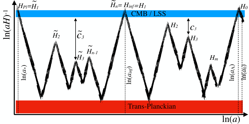
The initial condition and the eternity are the most debated subjects in the inflationary paradigm. In this note, we study these issues in the light of the TCC in the framework of multiple inflation. A generic scenario is illusterated in Fig. 1 and will be discussed in the following sections. The paper is structured as follows. In section II we see that a high scale observable inflation is consistent with the TCC. In section III we solve the initial condition problem for the observable inflation through introducing pre-inflations. In section IV we study power-law inflations precede and follow the plateau-like observable inflation. Finally, we conclude in section V.
II. Observable inflation at high-scale
In this section we study the case of high-scale observable inflation. First we compute the total number of e-folds needed to explain the horizon. Then, applying the TCC, we compute the Hubble rate for each inflationary epoch. In the end, we present a simple scenario.
The present horizon with multiple inflation
To address the the horizon problem, the present comoving Hubble horizon be inside the comoving horizon the the onset of observable inflation. If numerous inflations with scale happen then we find
| (6) | |||||
where index 1 indicates the observable inflation () and is the last one. In the third line we assume that a single stage with EoS parameter intervene between two inflations. For simplicity, we assume then the total number of e-folds satisfies
| (7) |
The upper bound on the Hubble parameters
We parametrize the ratio of the comoving horizon at the onset if each inflation to the present horizon as
| (8) |
The first inflation is assumed to be the observable one. It generates the CMB anisotropies and the gravitational waves. Thus, . On the other hand, the succedding inflations must not jeopardize the success of CMB observations which are in the range
| (9) |
Therefore, for . Moreover, if we happen to have a homogeneous patch before the onset of the first inflation, as the comoving Hubble volume never surpasses the initial one, the following inflations will follow without any further tuning.
For the final (th) stage of inflation we find that
| (10) | |||||
| (11) |
where in second line we assumed a single stage epoch. Applying the TCC inequality, we find an upper bound on the Hubble rate as
| (12) |
For the preceding inflations for , we find
| (13) | |||||
Similarly applying the TCC, we find an upper on
| (14) |
In particular, in the large limit, we find the upper bound on the observable inflation as
| (15) |
where we define the parameter . To see the importance of the above bound, we consider a special case with for . Assuming simple post-inflationary evolutions we find
| (16) |
A simple scenarion with high-scale inflation
If we take and assume matter-domination in between inflations , then
| (17) |
and (7) implies we need at least 48.8 e-folds. Applying (12) and (14) repeatedly we find
| (18) | |||||
| (19) | |||||
| (21) | |||||
| (22) |
Then, the Hubble rate of the final inflation is
| (23) |
(for MeV) and the number of e-folds is . Note that we would get the standard result of single inflation () so that GeV and .
The Hubble rate for the preceding one is
| (24) |
and the number of e-folds is bounded as . So far, we get e-folds. Note that, if this stage were the observable inflationary stage (), then we would have
| (25) |
and the number of e-folds would be bounded as . Thus the total number of e-folds is bounded by .
For the previous inflation we find
| (26) |
and the number of e-folds . It violates the bound from (17). Thus, it must be the observable (the first) inflation () with
| (27) |
and the number of e-folds . The total number of e-folds e-folds. This stage of inflation last for more than 7 e-folds and leave imprints on the CMB for scales spanning 3 orders of magnitude. Moreover, if the primordial gravitational waves are discovered in future measurements, then it can be accommodated in multiple-stage inflation.
III. Initial condition for the observable inflation
The scale of the observable inflation is at least three orders of magnitude below the Planck scale. If we define as the physical size of the smooth patch at the onset of inflation which is of order , and the corresponding length scale at the Planck time, then
| (28) |
In the above, is the EoS parameter of the fluid which takes over the Universe’s dynamics when it has emerged from the Planck era until the dawn of observable inflation. If we take GeV and then (unless ) the above equation implies that the physical volume of the Universe at the Planck time encompasses at least (for and for ) Hubble spheres with radius around Planck length. This is the initial condition for the observable inflation which must be granted if it is supposed to solve the initial condition problem of hot big bang model.
This problem can be alleviated via the very mechanism that solves the horizon problem of big bang model. After the Planck era, the universe follows an inflationary epoch with Hubble parameter close to the Planck scale. However, this inflation is not observable as we cannot observe modes that leave the horizon during this preiode. Besides, this cannot be prolonged as constrained by the TCC. In order to have a lower scale observable inflation with initial conditions set naturally at the Planck time without any fine-tuning we expect
| (29) |
Several epochs of inflation can happen in between the Planck scale one and the observable one. With a more convenient notation and , for stages of inflation we find
| (30) |
Assuming a simple inter-inflationary epoch we find
| (31) | |||||
| (32) |
where in the last line we assumed . Therefore,
| (33) |
and thus for matter-domination in intermediate stages (we would find around 4.6 e-folds for radiation domination).
To find the Hubble rates we parametrize the ratio of comoving horizon at the onset if each inflation () to the Planck horizon as
| (34) |
Then,
| (35) | |||||
| (36) |
Applying the TCC, we find a lower bound on the Hubble scale of the succeeding inflation as
| (37) |
If we assume the same EoS parameter for all inter-inflationary stages and parametrize () then we find the scale of succeeding inflation as follows
| (38) |
where
| (39) |
The number of e-folds for each stage of inflation is bounded by
| (40) |
for some arbitrary constant which turns the inequality in (38) into equality. The total number of e-folds, including the first one, is
| (41) |
where .
A simple sequence of pre-inflations
For matter domination and a simple model with , assuming we find , and which touches the Planck 2018 bound. Consequently, the TCC implies . Therefore, in order to set the initial conditions of the observable inflation, there need to be at least 3 epochs of inflation which in total provide around 3 e-folds. For radiation domination we find (), (). Although three inflations satisfy the lower bound (33), in order to satisfy the observational bound from non-detection of gravitations waves, we need at at least one more inflation before the observable one.
IV. Power-law assisting inflations
The lates results from the Planck satellite favors plateau-like (observable) inflation. However, as the other stages of inflations have no footprint on the CMB, they could be power-law in nature. In this section, we examine this scenario for early inflations and the late ones where the Universe is dominated by a fluid with EoS parameter . In this case, the Hubble rate the the beginning of inflation is not equal to the rate at the end of inflation . Therefore, using the dynamical equations in an expanding background, the TCC reads as follows
| (42) |
The results of this section match the results of the previous section for .It is convenient to define the following parameters
| (43) | |||||
| (44) |
where and and it can be large in the limit .
Inflation in early times
With power-law inflation, the minimum number of e-folds to set the initial smooth path of the observable inflation is computed as
| (46) | |||||
that can be compared to (31). For we find
| (47) |
For instance, for , in matter domination we obtain and in radiation domination we find . A stronger lower bound is obtained in the limit from below and from above.
To find the Hubble rates of power-law inflations, we parametrize the ratio of comoving Hubble horizons as
| (48) | |||||
| (49) |
Therefore, using the TCC relation (42) we find
| (50) |
We note that a single epoch of power-law inflation close to the Planck scale, with EoS can prepare the smooth patch of the observable inflation with Hubble rate 4 orders of magnitude less than the Planck scale. We parametrize and assum then
| (51) |
and the number of e-folds is . For and GeV we find (it never becomes more than ) .
Late times
To accommodate the present horizon with plateau-like observable inflation followed by multiple power-law ones we find a lower bound on the number of e-folds
| (53) | |||||
For the simple case we find the total number of e-folds as . It must obey (31).
For the final ( th) stage of inflation we find
| (54) | |||||
which after applying the TCC (42) implies
| (55) |
The Hubble rate for preceding inflations are bounded by
| (56) |
We recall that for the first stage .
We can model a simple two-stage inflation to explain the horizon. The observable one with EoS parameter is followed by a power-law inflation with EoS parameter determined by (56) as
| (57) |
The number of e-folds is bounded as
| (58) | |||||
| (59) |
For GeV we find that . The Hubble rate is around (less than) GeV. The number of e-folds is . Given that , the total number of e-folds is bounded as .
We find that a simple three stage inflation, starting from the Planck era, can happen naturally and explain the present horizon without any need of fine-tuning in initial conditions.
V. Conclusion
In this paper we revisit the framework of multiple inflationary scenario in light of the TCC. We found that high-scale inflations in the early times after the Planck era can prepare the initial conditions for the observable inflation. The observable inflation, can be of any scale and touch the Planck 2018 bound. If it is of high scale, then by the TCC, it cannot be prolonged and thus cannot solve the initial condition problem of the big bang model. However, we found that the succeeding inflations can explain the present horizon. All inflationary stages admit to the TCC. We also studied scenarios with a plateau-like observable inflation and supplementary power-law inflations. We found that in this scenario less number of inflations are needed provided that the EoS parameter during inflation is close to the critical value for the accelerated expansion. Eternal inflation is allowed in the framework of multi-inflation. We did not present any particular model and we describe the dynamics in terms of the effective EoS parameter of each epoch.
Acknowledgments
This work is supported by the research deputy of SUT.
∗ Electronic address: mahdi@physics.sharif.ir
References
- (1) A. A. Starobinsky, Phys. Lett. B 91 (1980) 99.
- (2) A. H. Guth, Phys. Rev. D 23 (1981) 347 [Adv. Ser. Astrophys. Cosmol. 3 (1987) 139]. doi:10.1103/PhysRevD.23.347
- (3) A. D. Linde, Phys. Lett. 108B, 389 (1982) [Adv. Ser. Astrophys. Cosmol. 3, 149 (1987)]. doi:10.1016/0370-2693(82)91219-9
- (4) A. Albrecht and P. J. Steinhardt, Phys. Rev. Lett. 48 (1982) 1220 [Adv. Ser. Astrophys. Cosmol. 3 (1987) 158]. doi:10.1103/PhysRevLett.48.1220
- (5) V. F. Mukhanov and G. V. Chibisov, JETP Lett. 33, 532 (1981) [Pisma Zh. Eksp. Teor. Fiz. 33, 549 (1981)].
- (6) V. F. Mukhanov and G. V. Chibisov, Sov. Phys. JETP 56, 258 (1982) [Zh. Eksp. Teor. Fiz. 83, 475 (1982)].
- (7) A. A. Starobinsky, Phys. Lett. 117B, 175 (1982). doi:10.1016/0370-2693(82)90541-X
- (8) C. L. Bennett et al., Astrophys. J. 464 (1996) L1 doi:10.1086/310075 [astro-ph/9601067].
- (9) G. Hinshaw et al. [WMAP Collaboration], Astrophys. J. Suppl. 208, 19 (2013) doi:10.1088/0067-0049/208/2/19 [arXiv:1212.5226 [astro-ph.CO]].
- (10) Y. Akrami et al. [Planck Collaboration], arXiv:1807.06205 [astro-ph.CO].
- (11) Y. Akrami et al. [Planck Collaboration], arXiv:1807.06211 [astro-ph.CO].
- (12) D. S. Goldwirth and T. Piran, Phys. Rev. Lett. 64 (1990) 2852. doi:10.1103/PhysRevLett.64.2852
- (13) D. S. Goldwirth and T. Piran, Phys. Rept. 214 (1992) 223. doi:10.1016/0370-1573(92)90073-9
- (14) A. Ijjas, P. J. Steinhardt and A. Loeb, Phys. Lett. B 723 (2013) 261 doi:10.1016/j.physletb.2013.05.023 [arXiv:1304.2785 [astro-ph.CO]].
- (15) A. H. Guth, D. I. Kaiser and Y. Nomura, Phys. Lett. B 733 (2014) 112 doi:10.1016/j.physletb.2014.03.020 [arXiv:1312.7619 [astro-ph.CO]].
- (16) A. Linde, doi:10.1093/acprof:oso/9780198728856.003.0006 arXiv:1402.0526 [hep-th].
- (17) D. Chowdhury, J. Martin, C. Ringeval and V. Vennin, Phys. Rev. D 100, no. 8, 083537 (2019) doi:10.1103/PhysRevD.100.083537 [arXiv:1902.03951 [astro-ph.CO]].
- (18) A. D. Linde, “Eternally Existing Selfreproducing Chaotic Inflationary Universe,” Phys. Lett. B 175 (1986) 395. doi:10.1016/0370-2693(86)90611-8
- (19) A. A. Starobinsky, “Stochastic De Sitter (Inflationary) Stage in the Early Universe,” Lect. Notes Phys. 246 (1986) 107. doi:10.1007/3-540-16452-9-6
- (20) M. Aryal and A. Vilenkin, “The Fractal Dimension of Inflationary Universe,” Phys. Lett. B 199 (1987) 351. doi:10.1016/0370-2693(87)90932-4
- (21) A. Vilenkin, Nucl. Phys. Proc. Suppl. 88 (2000) 67 doi:10.1016/S0920-5632(00)00755-6 [gr-qc/9911087].
- (22) A. H. Guth, Phys. Rept. 333, 555 (2000) doi:10.1016/S0370-1573(00)00037-5 [astro-ph/0002156].
- (23) A. Linde, Rept. Prog. Phys. 80, no. 2, 022001 (2017) doi:10.1088/1361-6633/aa50e4 [arXiv:1512.01203 [hep-th]].
- (24) C. Vafa, hep-th/0509212.
- (25) N. Arkani-Hamed, L. Motl, A. Nicolis and C. Vafa, JHEP 0706 (2007) 060 doi:10.1088/1126-6708/2007/06/060 [hep-th/0601001].
- (26) H. Ooguri and C. Vafa, Adv. Theor. Math. Phys. 21 (2017) 1787 doi:10.4310/ATMP.2017.v21.n7.a8 [arXiv:1610.01533 [hep-th]].
- (27) G. Obied, H. Ooguri, L. Spodyneiko and C. Vafa, arXiv:1806.08362 [hep-th].
- (28) S. K. Garg and C. Krishnan, JHEP 1911 (2019) 075 doi:10.1007/JHEP11(2019)075 [arXiv:1807.05193 [hep-th]].
- (29) H. Ooguri, E. Palti, G. Shiu and C. Vafa, Phys. Lett. B 788 (2019) 180 doi:10.1016/j.physletb.2018.11.018 [arXiv:1810.05506 [hep-th]].
- (30) H. Ooguri and C. Vafa, Nucl. Phys. B 766 (2007) 21 doi:10.1016/j.nuclphysb.2006.10.033 [hep-th/0605264].
- (31) D. Klaewer and E. Palti, JHEP 1701 (2017) 088 doi:10.1007/JHEP01(2017)088 [arXiv:1610.00010 [hep-th]].
- (32) E. Palti, Fortsch. Phys. 67 (2019) no.6, 1900037 doi:10.1002/prop.201900037 [arXiv:1903.06239 [hep-th]].
- (33) P. Agrawal, G. Obied, P. J. Steinhardt and C. Vafa, Phys. Lett. B 784 (2018) 271 doi:10.1016/j.physletb.2018.07.040 [arXiv:1806.09718 [hep-th]].
- (34) A. Achúcarro and G. A. Palma, JCAP 1902, 041 (2019) doi:10.1088/1475-7516/2019/02/041 [arXiv:1807.04390 [hep-th]].
- (35) A. Kehagias and A. Riotto, Fortsch. Phys. 66, no. 10, 1800052 (2018) doi:10.1002/prop.201800052 [arXiv:1807.05445 [hep-th]].
- (36) W. H. Kinney, S. Vagnozzi and L. Visinelli, Class. Quant. Grav. 36, no. 11, 117001 (2019) doi:10.1088/1361-6382/ab1d87 [arXiv:1808.06424 [astro-ph.CO]].
- (37) S. Brahma and M. Wali Hossain, JHEP 1903, 006 (2019) doi:10.1007/JHEP03(2019)006 [arXiv:1809.01277 [hep-th]].
- (38) S. Das, Phys. Rev. D 99, no. 8, 083510 (2019) doi:10.1103/PhysRevD.99.083510 [arXiv:1809.03962 [hep-th]].
- (39) G. Dvali and C. Gómez, Fortsch. Phys. 67 (2019) no.1-2, 1800092 doi:10.1002/prop.201800092 [arXiv:1806.10877 [hep-th]].
- (40) G. Dvali, C. Gómez and S. Zell, Fortsch. Phys. 67 (2019) no.1-2, 1800094 doi:10.1002/prop.201800094 [arXiv:1810.11002 [hep-th]].
- (41) T. Rudelius, JCAP 1908 (2019) 009 doi:10.1088/1475-7516/2019/08/009 [arXiv:1905.05198 [hep-th]].
- (42) H. Matsui and F. Takahashi, Phys. Rev. D 99 (2019) no.2, 023533 doi:10.1103/PhysRevD.99.023533 [arXiv:1807.11938 [hep-th]].
- (43) K. Dimopoulos, Phys. Rev. D 98 (2018) no.12, 123516 doi:10.1103/PhysRevD.98.123516 [arXiv:1810.03438 [gr-qc]].
- (44) W. H. Kinney, Phys. Rev. Lett. 122 (2019) no.8, 081302 doi:10.1103/PhysRevLett.122.081302 [arXiv:1811.11698 [astro-ph.CO]].
- (45) K. Andrzejewski and S. Prencel, Phys. Lett. B 782 (2018) 421 doi:10.1016/j.physletb.2018.05.072 [arXiv:1804.10979 [gr-qc]].
- (46) Z. Wang, R. Brandenberger and L. Heisenberg, arXiv:1907.08943 [hep-th].
- (47) A. Bedroya and C. Vafa, arXiv:1909.11063 [hep-th].
- (48) A. Bedroya, R. Brandenberger, M. Loverde and C. Vafa, arXiv:1909.11106 [hep-th].
- (49) Y. Cai and Y. S. Piao, arXiv:1909.12719 [gr-qc].
- (50) T. Tenkanen, arXiv:1910.00521 [astro-ph.CO].
- (51) S. Das, arXiv:1910.02147 [hep-th].
- (52) S. Mizuno, S. Mukohyama, S. Pi and Y. L. Zhang, arXiv:1910.02979 [astro-ph.CO].
- (53) S. Brahma, arXiv:1910.04741 [hep-th].
- (54) P. Draper and S. Farkas, arXiv:1910.04804 [hep-th].
- (55) M. Dhuria and G. Goswami, arXiv:1910.06233 [astro-ph.CO].
- (56) M. Torabian, arXiv:1910.06867 [hep-th].
- (57) R. G. Cai and S. J. Wang, arXiv:1910.07981 [astro-ph.CO].
- (58) K. Schmitz, arXiv:1910.08837 [hep-ph].
- (59) K. Kadota, C. S. Shin, T. Terada and G. Tumurtushaa, arXiv:1910.09460 [hep-th].
- (60) A. Berera and J. R. Calderón, arXiv:1910.10516 [hep-ph].
- (61) S. Brahma, arXiv:1910.12352 [hep-th].
- (62) G. Goswami and C. Krishnan, arXiv:1911.00323 [hep-th].
- (63) N. Okada, D. Raut and Q. Shafi, arXiv:1910.14586 [hep-ph].
- (64) W. C. Lin and W. H. Kinney, arXiv:1911.03736 [gr-qc].
- (65) H. H. Li, G. Ye, Y. Cai and Y. S. Piao, arXiv:1911.06148 [gr-qc].
- (66) A. Kehagias and A. Riotto, arXiv:1911.09050 [hep-th].
- (67) R. Saito, S. Shirai and M. Yamazaki, arXiv:1911.10445 [hep-th].
- (68) J. A. Adams, G. G. Ross and S. Sarkar, “Multiple Inflation,” Nucl. Phys. B 503 (1997) 405 doi:10.1016/S0550-3213(97)00431-8 [hep-ph/9704286].
- (69) N. Tetradis, Phys. Rev. D 57 (1998) 5997 doi:10.1103/PhysRevD.57.5997 [astro-ph/9707214].
- (70) C. P. Burgess, R. Easther, A. Mazumdar, D. F. Mota and T. Multamaki, JHEP 0505, 067 (2005) doi:10.1088/1126-6708/2005/05/067 [hep-th/0501125].
- (71) M. Kawasaki and K. Miyamoto, JCAP 1102 (2011) 004 doi:10.1088/1475-7516/2011/02/004 [arXiv:1010.3095 [astro-ph.CO]].
- (72) M. Cicoli, S. Downes, B. Dutta, F. G. Pedro and A. Westphal, JCAP 1412 (2014) 030 doi:10.1088/1475-7516/2014/12/030 [arXiv:1407.1048 [hep-th]].
- (73) K. Dimopoulos and M. Artymowski, Astropart. Phys. 94 (2017) 11 doi:10.1016/j.astropartphys.2017.06.006 [arXiv:1610.06192 [astro-ph.CO]].