跳到论文正文
W Papers独立论文阅读器 arXiv:1911.12042 论文正文 计算阅读时间 · 0%
引用这篇论文根据当前论文元数据生成,正式投稿前建议核对。


License: arXiv.org perpetual non-exclusive license
arXiv:1911.12042v1 [math.CO] 27 Nov 2019

Combinatorial model for mm-cluster categories in type EE

Bing Duan, Lisa Lamberti, Jian-Rong Li Address: Bing Duan, School of Mathematics and Statistics, Lanzhou University, Lanzhou, China Email address: duan890818@163.com Address: Lisa Lamberti, Department of Biosystems Science and Engineering, ETH Zürich, Basel, Switzerland; SIB Swiss Institute of Bioinformatics, Basel Switzerland Email address: lisa.lamberti@bsse.ethz.ch Address: Jian-Rong Li, Institute of Mathematics and Scientific Computing, University of Graz, Graz, Austria Email address: lijr07@gmail.com
Abstract.

In this paper, we revisit the geometric description of cluster categories in type EE in terms of colored diagonals in a polygon given in [17]. We then explain how the model generalizes to mm-cluster categories of the same type. As an application, we relate colored diagonals in a polygon to semi-standard Young tableaux, in type E6,E7,E8E_{6},E_{7},E_{8}. This provides a new compatibility description of semi–standard Young tableaux in Grassmannian cluster algebras in type E6,E8E_{6},E_{8} and in a sub-cluster algebra of type E7E_{7}.

1. Introduction

Understanding combinatorial patterns governing colored almost positive roots, i.e. copies of positive roots together with negative simple roots, in root systems is an interesting problem in the theory of cluster algebras. This problem has a wide range of implications, for instance, finding such descriptions allows to approximate similar patterns in larger root systems. The patterns we are referring to, are the ones arising in generalized cluster complexes and Coxeter combinatorics, or in mm-cluster categories (also called higher cluster categories) explored in a series of papers, see for example [8, 25, 28, 3, 4]. Despite various advancements in the field, to describe the usually infinite collection of maximally compatible sets of almost positive roots, resp.  of colored almost positive roots in general remains a difficult task, well understood only for classical type root systems.

In this paper, we make some progress in extending to the exceptional root systems in type EE and FF, combinatorial results obtained for the classical types A​B​C​DABCD. Specifically, in the first part (Section 3 and 4) we explore the link between colored almost positive roots in type EE and colored oriented mm-diagonals in polygons. In this way, we generalize to mm-cluster categories of type EE work of Thomas [25] and Baur–Marsh [3], relating mm-diagonals in a polytope to mm-cluster categories of type AA, and work of Lamberti [17] describing cluster categories of type EE in similar geometric terms.

In the second part, we revisit the relatively simple geometric model of colored diagonals suggested in [17] and related it to Young tableaux models. More specifically, Jensen, King, and Su in [13] gave a description of cluster variables in types E6,E8E_{6},E_{8} using some combinatorial objects called profiles. We describe cluster variables in types E6,E7,E8E_{6},E_{7},E_{8} using semi-standard Young tableaux, see Section 6. In particular, we present how the geometric model can be used to deduce compatibility of tableaux (Section 5 together with Section 6). Compatibility for almost positive roots is called cluster adjacency in physics, [7, 18, 20] and has important applications to the theory of scattering amplitude in physics.

Acknowledgements

B. Duan is supported by the National Natural Science Foundation of China (no. 11771191). L. Lamberti would like to thank B. Zhu for a question asked at the Korean Institute for Advanced Studies during a Conference on Cluster Algebras and Representation Theory in 2014 leading to the geometric model for mm-cluster categories presented in Section 3. J.-R. Li is supported by the Austrian Science Fund (FWF): M 2633-N32 Meitner Program.

2. Preliminaries on mm-cluster categories and Grassmannian cluster algebras

In this section we define orbit categories of representations of valued quivers following [28] closely. In this work, however, we will mostly focus on representations of ordinary simply-laced Dynkin quivers in types E6,E7E_{6},E_{7} and E8E_{8}. Results for mm-cluster categories in type F4F_{4} are deduced by a folding argument.

2.1. Definition of mm-cluster categories

Let (G,d)(G,d) be a valued graph. That is, a finite set of vertices [n]={1,…,n}[n]=\{1,\ldots,n\} together with nonnegative integers di​jd_{ij} for all pairs of vertices i,j∈[n]×[n]i,j\in[n]\times[n] such that di​i=0d_{ii}=0 and positive integers {ϵi}i∈G\{\epsilon_{i}\}_{i\in G} satisfying

di​j​ϵj=dj​i​ϵid_{ij}\epsilon_{j}=d_{ji}\epsilon_{i}

for all i,j∈[n]i,j\in[n]. An edge in (G,d)(G,d) is a pair {i,j}\{i,j\} with di​j≠0d_{ij}\neq 0. An orientation Σ\Sigma of (G,d)(G,d) is given by assigning to each edge in (G,d)(G,d) an order. Denote an oriented valued quiver by (G,Σ)(G,\Sigma). Throughout it is assumed that (G,Σ)(G,\Sigma) has no oriented cycles. Let Φ\Phi be the root system of the Kac–Moody Lie algebra corresponding to GG. If for each arrow in (G,Σ)(G,\Sigma) one has that ϵj=ϵi\epsilon_{j}=\epsilon_{i}, (G,Σ)(G,\Sigma) is an ordinary quiver, simply denoted by QQ.

Let kk be an algebraically closed field and let M=(Fi,Mji)i,j∈GM=(F_{i},{}_{i}M_{j})_{i,j\in G} be a reduced kk-species of (G,Σ)(G,\Sigma). That is, for all i,j∈[n]i,j\in[n], Mji{}_{i}M_{j} is an Fi−FjF_{i}-F_{j}-bimodule, where FiF_{i} and FjF_{j} are division rings which are finite dimensional vector spaces over kk and dim⁡(Mji)=di,j\mathrm{dim}({}_{i}M_{j})=d_{i,j} and dimkFi=ϵi\dim_{k}F_{i}=\epsilon_{i}. Let the category of finite-dimensional representations of (G,Σ,M)(G,\Sigma,M) be denoted by ℋ\mathcal{H}. Let 𝒟:=𝒟⁡(ℋ)\mathcal{D}:=\mathcal{D}(\mathcal{H}) be the bounded derived category of the abelian category ℋ\mathcal{H} endowed with shift functor Σ:𝒟→𝒟\Sigma:\mathcal{D}\rightarrow\mathcal{D} and Auslander–Reiten translation τ:𝒟→𝒟\tau:\mathcal{D}\rightarrow\mathcal{D}, defined as Hom𝒟​(X,−)∗≅Hom𝒟​(−,Σ​τ​X),\mathrm{Hom}_{\mathcal{D}}(X,-)^{*}\cong\mathrm{Hom}_{\mathcal{D}}(-,\Sigma\tau X), for all X∈𝒟X\in\mathcal{D}.

For m∈ℤ≥1m\in\mathbb{Z}_{\geq 1}, define the mm-cluster category of type Φ\Phi as the orbit category:

𝒞Φm=𝒟/⟨τ−1​Σm⟩.\mathcal{C}^{m}_{\Phi}=\mathcal{D}/\langle\tau^{-1}\Sigma^{m}\rangle.

Objects are the (τ−1​Σm)(\tau^{-1}\Sigma^{m})-orbits of objects in 𝒟\mathcal{D} and morphisms are defined by

Hom𝒞Φm​(X~,Y~)=⨁i∈ℤHom𝒟​((τ−1​Σm)i​X,Y)\mathrm{Hom}_{\mathcal{C}^{m}_{\Phi}}(\widetilde{X},\widetilde{Y})=\bigoplus_{i\in\mathbb{Z}}\mathrm{Hom}_{\mathcal{D}}\Big((\tau^{-1}\Sigma^{m})^{i}X,Y\Big)

where X~\widetilde{X} and Y~\widetilde{Y} are representatives of the τ−1​Σm\tau^{-1}\Sigma^{m}-orbits of XX and YY respectively. In the above, Σm\Sigma^{m} denotes the composition of Σ\Sigma with itself mm-times. It is known that 𝒞Φm\mathcal{C}^{m}_{\Phi} is again a triangulated category, [14, Theorem 1], with shift Σ\Sigma and Serre functor τ​Σ\tau\Sigma induced from 𝒟\mathcal{D}. Moreover, 𝒞Φm\mathcal{C}^{m}_{\Phi} is Krull-Schmidt with finite dimensional Hom\mathrm{Hom}-spaces and (m+1)(m+1)-Calabi Yau, see for instance [28, Prop 2.2].

2.2. Isomorphisms of stable translation quivers

A quiver Γ\Gamma without loops nor multiple edges, together with a bijective map τ:Γ→Γ\tau:\Gamma\rightarrow\Gamma, is a stable translation quiver (Γ,τ)(\Gamma,\tau), in the sense of [22], if τ\tau is such that for all vertices xx in Γ\Gamma the set of starting points of arrows which end in xx is equal to the set of end points of arrows which start at τ⁡(x)\tau(x). The map τ\tau is called translation. For a stable translation quiver (Γ,τ)(\Gamma,\tau) one defines the mesh category of (Γ,τ)(\Gamma,\tau) as the quotient category of the additive path category of Γ\Gamma by the mesh ideal, see [15] for details on this construction.

Let QQ be an ordinary quiver. Let (ℤ​Q,τ)(\mathbb{Z}Q,\tau) be the stable translation quiver given by the repetitive quiver of QQ, defined as in [12, I, 5.6]. Let τ:ℤ​Q→ℤ​Q\tau:\mathbb{Z}Q\rightarrow\mathbb{Z}Q be defined on the vertices (n,i)(n,i) of ℤ​Q\mathbb{Z}Q by τ⁡(n,i)=(n−1,i)\tau(n,i)=(n-1,i), for n∈ℤn\in\mathbb{Z}, ii a vertex in QQ.

We recall, the Auslander–Reiten quiver of any Krull–Schmidt category 𝒦\mathcal{K} is a quiver whose vertices are the (isomorphism classes of) indecomposable objects in 𝒦\mathcal{K}. The number of arrows between two vertices XX and YY is given by the dimension of the space of irreducible morphisms between XX and YY:

Irr𝒦​(X,Y):=rad⁡(X,Y)/rad2​(X,Y).\mathrm{Irr}_{\mathcal{K}}(X,Y):=\mathrm{rad}(X,Y)/\mathrm{rad}_{2}(X,Y).

Here rad⁡(X,Y)⊂Hom𝒦​(X,Y)\mathrm{rad}(X,Y)\subset\mathrm{Hom}_{\mathcal{K}}(X,Y) consists of all non-isomorphisms, and rad2​(X,Y)⊂rad⁡(X,Y)\mathrm{rad}_{2}(X,Y)\subset\mathrm{rad}(X,Y) consists of non-isomorphisms admitting a non-trivial factorization. Denote the Auslander–Reiten quiver of the orbit category 𝒞Φm\mathcal{C}^{m}_{\Phi} with Auslander–Reiten translation τ\tau by (ΓΦm,τ)(\Gamma_{\Phi}^{m},\tau). If m=1m=1, the index mm will be omitted.

For QQ of type E6E_{6} let ρ:ℤ​E6→ℤ​E6\rho:\mathbb{Z}{E_{6}}\rightarrow\mathbb{Z}{E_{6}} be the order two involution given by the horizontal reflexion along the center line of ℤ​E6\mathbb{Z}E_{6}. For m∈ℤ≥1,m\in\mathbb{Z}_{\geq 1}, let ρm\rho^{m} be the composition of ρ\rho with itself mm-times.

Lemma 2.1.

Let QQ be of type E6,E7,E8E_{6},E_{7},E_{8}, then the following are isomorphisms of stable translation quivers:

  • •

    (ΓE6m,τ)≅(ℤ​E6/τ−(6​m+1)​ρm,τ)(\Gamma_{E_{6}}^{m},\tau)\cong(\mathbb{Z}E_{6}/\tau^{-(6m+1)}\rho^{m},\tau)

  • •

    (ΓE7m,τ)≅(ℤ​E7/τ−(9​m+1),τ)(\Gamma_{E_{7}}^{m},\tau)\cong(\mathbb{Z}E_{7}/\tau^{-(9m+1)},\tau)

  • •

    (ΓE8m,τ)≅(ℤ​E8/τ−(15​m+1),τ)(\Gamma_{E_{8}}^{m},\tau)\cong(\mathbb{Z}E_{8}/\tau^{-(15m+1)},\tau)

Proof.

The claim follows from Happel’s result, see [12, I.5.5] together with the description of the induced action of the functors τ\tau and Σ\Sigma on ℤ​Q\mathbb{Z}Q, first given in [21, Chap. 4]. Specifically, the induced action of τ\tau on ℤ​Q\mathbb{Z}Q is always an horizontal shift to the left. The induced action of Σ\Sigma on ℤ​An\mathbb{Z}A_{n} can be described by a shift of n+12\frac{n+1}{2} steps to the right, composed with a reflection along the horizontal central line of ℤ​An\mathbb{Z}A_{n}. When nn is even, the steps are not required to be integer units. The action of Σ\Sigma on ℤ​E6\mathbb{Z}E_{6} coincides with the action of ρ​τ−6\rho\tau^{-6} on ℤ​E6\mathbb{Z}E_{6}. Moreover, Σ\Sigma acts as τ−9\tau^{-9} on ℤ​E7\mathbb{Z}E_{7}, and as τ−15\tau^{-15} on ℤ​E8\mathbb{Z}E_{8}. ∎

The case of (ΓF4m,τ)(\Gamma_{F_{4}}^{m},\tau) follows from (ΓE6m,τ)(\Gamma_{E_{6}}^{m},\tau) via a standard folding argument.

2.3. Cluster tilting theory in mm-cluster categories

Work of Thomas [25] (for simply laced cases) and of Zhu’s [28] (general case) describe the combinatorics of cluster tilting objects in mm-cluster categories associated to valued quivers. We now recollect a few results from [25, 28].

Definition 2.2.
  • •

    An object T∈𝒞ΦmT\in\mathcal{C}^{m}_{\Phi} is called mm-rigid if it is the direct sum of non isomorphic indecomposable objects T1,…,TtT_{1},\dots,T_{t} such that Ext𝒞Φmi​(Tj,Tk)=0\mathrm{Ext}^{i}_{\mathcal{C}^{m}_{\Phi}}(T_{j},T_{k})=0 for all 1≤i≤m,1\leq i\leq m, and 1≤j,k≤t1\leq j,k\leq t. It is called maximal mm-rigid if it is mm-rigid and maximal with respect to this property.

  • •

    An object T∈𝒞ΦmT\in\mathcal{C}^{m}_{\Phi} is an mm-cluster tilting object which is maximal mm-rigid and X∈add​TX\in\mathrm{add}T if and only if Ext𝒞Φmi​(T,X)=0\mathrm{Ext}^{i}_{\mathcal{C}^{m}_{\Phi}}(T,X)=0 for 1≤i≤m1\leq i\leq m.

To exhaustively search for mm-cluster tilting objects in mm-cluster categories, it is crucial to know how many objects of this type there are in a fixed mm-cluster category. The next result gives an explicit answer for mm-cluster categories associated to valued quivers.

Theorem 2.3 ([8, 28]).

Let QQ be an orientation of a connected Dynkin diagram and Φ\Phi the corresponding root system. The number of mm-cluster tilting objects in 𝒞Φm\mathcal{C}^{m}_{\Phi} is

∏im​h+ei+1ei+1\prod_{i}\frac{mh+e_{i}+1}{e_{i}+1}

where hh is the Coxeter number of Φ\Phi, and e1,…,ene_{1},\dots,e_{n} are the exponents of Φ\Phi.

Theorem 2.3 follows from [8, Prop. 8.4] as described in [28, Cor. 5.8]. The exponents in the next Table are extracted from [8].

Φ\Phi hh Exponents 22-cluster tilting objects
E6E_{6} 12 1,4,5,7,8,11 16.588
F4F_{4} 12 1,5,7,11 780
E7E_{7} 18 1,5,7,9,11,13,17 144.210
E8E_{8} 30 1,7,11,13,17,19,23,29 15.209.220

2.4. Colored almost positive roots

Let Φ\Phi be an irreducible root system of rank nn, associated to a valued graph, or quiver. Let II be an nn-element indexing set. Let Φ>0\Phi_{>0} be the set of positive roots and let {αi:i∈I}\{\alpha_{i}:i\in I\} be the set of simple roots in Φ\Phi. Following [8] we define the set of almost positive roots in Φ\Phi as

Φ≥−1=Φ>0∪{−αi:i∈I}.\Phi_{\geq-1}=\Phi_{>0}\ \cup\ \{-\alpha_{i}:i\in I\}.

For m∈ℤ>0m\in\mathbb{Z}_{>0}, the set of colored almost positive roots consists of mm-copies of the set Φ>0\Phi_{>0} together with one copy of the negative simple roots in Φ\Phi, i.e.:

Φ≥−1m=Φ>0∪…∪Φ>0⏟m−copies∪{−αi:i∈I}.\Phi^{m}_{\geq-1}=\underbrace{\Phi_{>0}\ \cup\ \dots\ \cup\ \Phi_{>0}}_{m-\textrm{copies}}\ \cup\ \{-\alpha_{i}:i\in I\}.

When m=1m=1, the index in Φ≥−1m\Phi^{m}_{\geq-1} is omitted. The compatibility degree of mm-colored almost positive roots is defined in [8, Def 3.1].

On the one side, work of Thomas [25, §.6] describes a correspondence between mm-colored almost positive roots and indecomposable objects in a geometrically defined mm-cluster category associated to Φ\Phi. The compatibility degree of mm-colored almost positive roots can then equivalently be computed via Ext\mathrm{Ext}-functors in mm-cluster categories [25, Prop. 2]. The non-simply laced case was described in work of Zhu [28, §.5] and [28, §.5, Def. 5.2]. When m=1m=1 and QQ is of finite Dynkin type, this property is shown in [5, Prop. 4.2], [27].

On the other side, work of Fomin–Reading [8, §.5] implies that there is a one-to-one correspondence between mm-diagonals in certain polygons Π\Pi and mm-colored almost positive roots Φ≥−1m\Phi_{\geq-1}^{m} of type A​B​C​DABCD. See also work of Tzanaki [26] for types A​B.AB.

In the above settings, two colored almost positive roots α\alpha and β\beta are compatible, if the corresponding mm-diagonals DαD_{\alpha} and DβD_{\beta} do not cross. When m=1,m=1, these descriptions coincide with the ones given in [10, §.3.5].

2.5. The mm-power of a translation quiver

Colored almost positive roots in a root system of type AA can be identified with a subset of almost positive roots in a larger root system of the same type, see for instance [25, 8, 26]. In [3] this relationship is described in terms of an mm-power operation. We now extend this approach to mm-cluster categories of type EE.

Definition 2.4.

Let (Γ,τ)(\Gamma,\tau) be a translation quiver. The quiver (Γ)m(\Gamma)^{m} whose vertices are the same as the ones from Γ\Gamma and whose arrows are sectional paths of length mm is called the mm-th power of Γ\Gamma. A path (x=x0→x1→…→xm−1→xm=y)(x=x_{0}\rightarrow x_{1}\rightarrow...\rightarrow x_{m-1}\rightarrow x_{m}=y) in Γ\Gamma is said to be sectional if τ​xi+1≠xi−1\tau x_{i+1}\neq x_{i-1} for i=1,…,m−1i=1,...,m-1 (for which τ​xi+1\tau x_{i+1} is defined).

Lemma 2.5.

If (Γ,τ)(\Gamma,\tau) is a stable translation quiver, then ((Γ)m,τm)((\Gamma)^{m},\tau^{m}) for τm:=τ∘…∘τ,\tau^{m}:=\tau\circ...\circ\tau, composed mm times, is again a stable translation quiver.

Proof.

This is shown in Theorem 6.1 in [3] and Corollary 6.2 in [3]. ∎

Let Tr,s,tT_{r,s,t} be an orientation of a finite connected graph with r+s+t+1r+s+t+1 vertices and three legs. Assume that one vertex of Tr,s,tT_{r,s,t} has three neighbors and that the legs of Tr,s,tT_{r,s,t} have rr, resp. ss, resp. tt vertices. A tree Tr,s,tT_{r,s,t} is symmetric if two legs have the same number of vertices.

Below, for i∈{6,7,8}i\in\{6,7,8\}, let (ΓEim,τ)(\Gamma_{E_{i}}^{m},\tau) be as described in Lemma 2.1.

Proposition 2.6.

The following quivers are connected components of the mm-power of the given stable translation quivers:

  • •

    (ΓE6m,τm)⊆(ℤ​T2​m−1,2​m,2​m/τ−(6​m+1)​ρm)m(\Gamma_{E_{6}}^{m},\tau^{m})\subseteq(\mathbb{Z}T_{2m-1,2m,2m}/\tau^{-(6m+1)}\rho^{m})^{m}

  • •

    (ΓE7m,τm)⊆(ℤ​T2​m−1,2​m,3​m/τ−(9​m+1))m(\Gamma_{E_{7}}^{m},\tau^{m})\subseteq(\mathbb{Z}T_{2m-1,2m,3m}/\tau^{-(9m+1)})^{m}

  • •

    (ΓE8m,τm)⊆(ℤ​T2​m−1,2​m,4​m/τ−(15​m+1))m(\Gamma_{E_{8}}^{m},\tau^{m})\subseteq(\mathbb{Z}T_{2m-1,2m,4m}/\tau^{-(15m+1)})^{m}

Proof.

Lemma 2.1 describes the shapes of the quiver (ΓEim,τ)(\Gamma_{E_{i}}^{m},\tau), for i∈{6,7,8}i\in\{6,7,8\}. Reversing the mm-power procedure, by adding meshes in the quivers ΓEim\Gamma_{E_{i}}^{m}, for i∈{6,7,8}i\in\{6,7,8\} gives rise to the larger quivers in the claim. ∎

2.5.1. Geometric categories associated to tree diagrams

Let Tr,s,tT_{r,s,t} be a fixed tree diagram. For n≥max⁡{r+s+1;r+t+1}n\geq\mathrm{max}\{r+s+1;r+t+1\} let Πr,s,t\Pi_{r,s,t} be a regular (n+3)(n+3)-gon with vertices numbered in the clockwise order by the group ℤ/(n+3)​ℤ\mathbb{Z}/(n+3)\mathbb{Z}.

For the vertices i,j,ki,j,k in Πr,s,t\Pi_{r,s,t} we write i≤j≤ki\leq j\leq k if the vertex jj is between ii and kk in the clockwise order. A diagonal in Πr,s,t\Pi_{r,s,t} joining the vertices ii and jj is denoted by (i,j)(i,j) and an oriented diagonal in Πr,s,t\Pi_{r,s,t} starting at ii and ending in jj is denoted by [i,j][i,j]. Boundary segments are not considered.

Following [17], we associate to each leg in Tr,s,tT_{r,s,t} a set of diagonals in Πr,s,t\Pi_{r,s,t}. To do so, we double the set of all oriented diagonals in Πr,s,t\Pi_{r,s,t}, and distinguish them with colors, red and blue, and subscripts RR, BB. Specifically, for every vertex ii in Πr,s,t\Pi_{r,s,t} we then form (r+1)(r+1) pairs of colored oriented diagonals:

[i,i+2]P=\displaystyle[i,i+2]_{P}= [i+2,i]P:={[i,i+2]R,[i+2,i]B}\displaystyle[i+2,i]_{P}:=\{[i,i+2]_{R},[i+2,i]_{B}\}
[i,i+3]P=\displaystyle[i,i+3]_{P}= [i+3,i]P:={[i,i+3]R,[i+3,i]B}\displaystyle[i+3,i]_{P}:=\{[i,i+3]_{R},[i+3,i]_{B}\}
…\displaystyle\dots
[i,i+r+2]P=\displaystyle[i,i+r+2]_{P}= [i+r+2,i]P:={[i,i+r+2]R,[i+r+2,i]B}.\displaystyle[i+r+2,i]_{P}:=\{[i,i+r+2]_{R},[i+r+2,i]_{B}\}.

As before, coordinates are viewed as elements of ℤ/(n+3)​ℤ.\mathbb{Z}/(n+3)\mathbb{Z}. Once colored oriented diagonals are paired, they stop existing as single diagonals in Πr,s,t\Pi_{r,s,t}. In the following, we color paired diagonals in green.

Next, one defines a subset of the diagonals of Πr,s,t\Pi_{r,s,t} consisting of (r+1)​(n+3)(r+1)(n+3) paired, s⁡(n+3)s(n+3) single red and t⁡(n+3)t(n+3) single blue oriented diagonals:

Pr,s,t:={\displaystyle P_{r,s,t}:=\bigg\{ [i,i+2]G,…,[i,i+r+2]G,\displaystyle[i,i+2]_{G},\dots,[i,i+r+2]_{G},
[i,i+r+3]R,…,[i,i+r+s+2]R,\displaystyle[i,i+r+3]_{R},\dots,[i,i+r+s+2]_{R},
[i+r+3,i]B,…,[i+r+t+2,i]B, i vertex of Πr,s,t}.\displaystyle[i+r+3,i]_{B},\dots,[i+r+t+2,i]_{B},\hskip 8.5359pt\textrm{ $i$ vertex of }\Pi_{r,s,t}\bigg\}.

The set of red, blue and green diagonals of Πr,s,t\Pi_{r,s,t} are disjoint. Consequently, orientations can now be omitted. Elements in Pr,s,tP_{r,s,t} are henceforth called colored diagonals.

2.5.2. Automorphisms on the set of colored diagonals

Let ρ,τ0\rho,\tau_{0} and τ\tau be automorphisms acting on the set of colored diagonals Pr,s,tP_{r,s,t} of Πr,s,t\Pi_{r,s,t} associated to a tree Tr,s,tT_{r,s,t}. The first two automorphisms are non-trivial only when Tr,s,tT_{r,s,t} is symmetric. While the automorphism τ:Pr,s,t→Pr,s,t\tau:P_{r,s,t}\rightarrow P_{r,s,t} is always given as the anti-clockwise rotation through 2​πn+3\frac{2\pi}{n+3} around the center of Π\Pi.

For c∈{R,B,G}c\in\{R,B,G\}, let ρ:Pr,t,t→Pr,t,t\rho:P_{r,t,t}\rightarrow P_{r,t,t} be the automorphism of order two given by

ρ⁡([i,j]c):={[j,i]Bif ​c=R,[j,i]Rif ​c=B,[i,j]Gotherwise.\rho\big([i,j]_{c}\big):=\begin{cases}[j,i]_{B}&\textrm{if }c=R,\\ [j,i]_{R}&\textrm{if }c=B,\\ [i,j]_{G}&\textrm{otherwise.}\end{cases}

The definition of τ0:Pr,t,t→Pr,t,t\tau_{0}:P_{r,t,t}\rightarrow P_{r,t,t} is designed to accommodate the action of the shift functor on the mm-cluster category of type E6E_{6}:

τ0​([i,j]c):={ρ⁡([i−1,j−1]c) if ​[i,j]c∈Pr,t,t|1[i−1,j−1]c otherwise.\tau_{0}([i,j]_{c}):=\begin{cases}\rho\big([i-1,j-1]_{c}\big)&\textrm{ if }[i,j]_{c}\in P_{r,t,t}|_{1}\\ [i-1,j-1]_{c}&\textrm{ otherwise.}\end{cases}

Here Pr,t,t|1⊂Pr,t,tP_{r,t,t}|_{1}\subset P_{r,t,t} denotes the set of diagonals starting, resp. ending, at the fixed vertex i=1i=1.

2.5.3. Minimal clockwise rotations

The definition of minimal clockwise rotation of elements of Πr,s,t\Pi_{r,s,t} changes in the presence of ρ\rho. First, consider the case where Tr,s,tT_{r,s,t} is not symmetric, or when Tr,t,tT_{r,t,t} is symmetric and τ\tau is the standard anti-clockwise rotation. Then the minimal clockwise rotations are the standard ones. That is, for k,jk,j non-neighboring vertices and for c∈{R,B,G}c\in\{R,B,G\}, the minimal clockwise rotation among diagonals in Pr,s,tP_{r,s,t} is defined by: [k,j]c→[k,j+1]c[k,j]_{c}\rightarrow[k,j+1]_{c} and [k,j]c→[k+1,j]c[k,j]_{c}\rightarrow[k+1,j]_{c} and if j∈{k+r+2,k+r+3}j\in\{k+r+2,k+r+3\} by:

    [k,k+r+3]R          [k,k+r+2]G               [k+1,k+r+3]G.   [k+r+3,k]B          .\lx@xy@svg{\hbox{\raise 2.5pt\hbox{\kern 3.0pt\hbox{\ignorespaces\ignorespaces\ignorespaces\hbox{\vtop{\halign{\entry@#!@&&\entry@@#!@\cr&&&&\cr&&&\cr&&&&\crcr}}}\ignorespaces{\hbox{\kern-3.0pt\raise 0.0pt\hbox{\hbox{\kern 0.0pt\raise 0.0pt\hbox{\hbox{\kern 3.0pt\raise-2.5pt\hbox{$\textstyle{}$}}}}}}}{\hbox{\kern 40.00066pt\raise 0.0pt\hbox{\hbox{\kern 0.0pt\raise 0.0pt\hbox{\hbox{\kern 3.0pt\raise-2.5pt\hbox{$\textstyle{}$}}}}}}}{\hbox{\kern 83.16277pt\raise 0.0pt\hbox{\hbox{\kern 0.0pt\raise 0.0pt\hbox{\hbox{\kern 3.0pt\raise-2.5pt\hbox{$\textstyle{[k,k+r+3]_{R}\ignorespaces\ignorespaces\ignorespaces\ignorespaces}$}}}}}}}\ignorespaces\ignorespaces\ignorespaces{}\ignorespaces\ignorespaces{\hbox{\lx@xy@drawline@}}\ignorespaces{\hbox{\kern 157.15964pt\raise-6.69522pt\hbox{\hbox{\kern 0.0pt\raise 0.0pt\hbox{\lx@xy@tip{1}\lx@xy@tip{-1}}}}}}\ignorespaces\ignorespaces{\hbox{\lx@xy@drawline@}}\ignorespaces{\hbox{\lx@xy@drawline@}}{\hbox{\kern 198.16026pt\raise 0.0pt\hbox{\hbox{\kern 0.0pt\raise 0.0pt\hbox{\hbox{\kern 3.0pt\raise-2.5pt\hbox{$\textstyle{}$}}}}}}}{\hbox{\kern 251.16089pt\raise 0.0pt\hbox{\hbox{\kern 0.0pt\raise 0.0pt\hbox{\hbox{\kern 3.0pt\raise-2.5pt\hbox{$\textstyle{}$}}}}}}}{\hbox{\kern-3.0pt\raise-14.0pt\hbox{\hbox{\kern 0.0pt\raise 0.0pt\hbox{\hbox{\kern 3.0pt\raise-2.5pt\hbox{$\textstyle{}$}}}}}}}{\hbox{\kern 9.0pt\raise-14.0pt\hbox{\hbox{\kern 0.0pt\raise 0.0pt\hbox{\hbox{\kern 3.0pt\raise-2.5pt\hbox{$\textstyle{[k,k+r+2]_{G}\ignorespaces\ignorespaces\ignorespaces\ignorespaces\ignorespaces\ignorespaces\ignorespaces\ignorespaces}$}}}}}}}\ignorespaces\ignorespaces\ignorespaces{}\ignorespaces\ignorespaces\ignorespaces{\hbox{\kern 83.16277pt\raise-6.42581pt\hbox{\hbox{\kern 0.0pt\raise 0.0pt\hbox{\lx@xy@tip{1}\lx@xy@tip{-1}}}}}}\ignorespaces\ignorespaces{\hbox{\lx@xy@drawline@}}\ignorespaces\ignorespaces\ignorespaces\ignorespaces{}\ignorespaces\ignorespaces{\hbox{\lx@xy@drawline@}}\ignorespaces{\hbox{\kern 83.00131pt\raise-21.57689pt\hbox{\hbox{\kern 0.0pt\raise 0.0pt\hbox{\lx@xy@tip{1}\lx@xy@tip{-1}}}}}}\ignorespaces\ignorespaces{\hbox{\lx@xy@drawline@}}\ignorespaces{\hbox{\lx@xy@drawline@}}{\hbox{\kern 114.08047pt\raise-14.0pt\hbox{\hbox{\kern 0.0pt\raise 0.0pt\hbox{\hbox{\kern 3.0pt\raise-2.5pt\hbox{$\textstyle{}$}}}}}}}{\hbox{\kern 157.15964pt\raise-14.0pt\hbox{\hbox{\kern 0.0pt\raise 0.0pt\hbox{\hbox{\kern 3.0pt\raise-2.5pt\hbox{$\textstyle{[k+1,k+r+3]_{G}.}$}}}}}}}{\hbox{\kern-3.0pt\raise-28.0pt\hbox{\hbox{\kern 0.0pt\raise 0.0pt\hbox{\hbox{\kern 3.0pt\raise-2.5pt\hbox{$\textstyle{}$}}}}}}}{\hbox{\kern 40.00066pt\raise-28.0pt\hbox{\hbox{\kern 0.0pt\raise 0.0pt\hbox{\hbox{\kern 3.0pt\raise-2.5pt\hbox{$\textstyle{}$}}}}}}}{\hbox{\kern 83.00131pt\raise-28.0pt\hbox{\hbox{\kern 0.0pt\raise 0.0pt\hbox{\hbox{\kern 3.0pt\raise-2.5pt\hbox{$\textstyle{[k+r+3,k]_{B}\ignorespaces\ignorespaces\ignorespaces\ignorespaces}$}}}}}}}\ignorespaces\ignorespaces\ignorespaces{}\ignorespaces\ignorespaces{\hbox{\lx@xy@drawline@}}\ignorespaces{\hbox{\kern 157.15964pt\raise-21.34775pt\hbox{\hbox{\kern 0.0pt\raise 0.0pt\hbox{\lx@xy@tip{1}\lx@xy@tip{-1}}}}}}\ignorespaces\ignorespaces{\hbox{\lx@xy@drawline@}}\ignorespaces{\hbox{\kern 198.16026pt\raise-28.0pt\hbox{\hbox{\kern 0.0pt\raise 0.0pt\hbox{\hbox{\kern 3.0pt\raise-2.5pt\hbox{$\textstyle{}$}}}}}}}{\hbox{\kern 251.16089pt\raise-28.0pt\hbox{\hbox{\kern 0.0pt\raise 0.0pt\hbox{\hbox{\kern 3.0pt\raise-2.5pt\hbox{$\textstyle{}$}}}}}}}\ignorespaces}}}}\ignorespaces.

Second, when Tr,t,tT_{r,t,t} is symmetric and the translation is τ0\tau_{0}, the minimal clockwise rotations are defined as before except when [k,j]c[k,j]_{c}, [k,k+r+2]G[k,k+r+2]_{G} are in τ0​(Pr,t,t|1)\tau_{0}(P_{r,t,t}|_{1}), then one combines the minimal clockwise rotation with ρ\rho.

2.5.4. Quivers of single and paired colored oriented diagonals

Let Γr,s,tn+3\Gamma^{n+3}_{r,s,t} be the quiver whose vertices are the elements of Pr,s,tP_{r,s,t}. An arrow between two vertices of Γr,s,tn+3\Gamma^{n+3}_{r,s,t} is drawn whenever there is a minimal clockwise rotation linking them. No arrow is drawn otherwise. In this way Γr,s,tn+3\Gamma^{n+3}_{r,s,t} lies on a cylinder, unless when s=ts=t and the translation is given by τ0\tau_{0}. Then Γr,t,tn+3\Gamma^{n+3}_{r,t,t} lies on a Möbius strip.

Lemma 2.7.

[17, Lemma 4.1] The quivers (Γr,s,tn+3,τ)(\Gamma_{r,s,t}^{n+3},\tau) and (Γr,t,tn+3,τ0)(\Gamma_{r,t,t}^{n+3},\tau_{0}) are stable translation quivers. ∎

2.5.5. Folded quiver Γr,tn+3\Gamma^{n+3}_{r,t}

When the quiver (Γr,t,tn+3,τ)({\Gamma}^{n+3}_{r,t,t},\tau), resp.  (Γr,t,tn+3,τ0)({\Gamma}^{n+3}_{r,t,t},\tau_{0}), are symmetric along its horizontal central line, folding produces a new translation quiver which we denote by (Γr,tn+3,τ)(\Gamma^{n+3}_{r,t},\tau). More precisely, consider again the graph automorphism ρ\rho. The vertices of Γr,tn+3\Gamma^{n+3}_{r,t} are the ρ\rho-orbits of vertices of Γr,t,tn+3\Gamma^{n+3}_{r,t,t}. The arrows in Γr,tn+3\Gamma^{n+3}_{r,t} are always single and coincide with minimal clockwise rotation around a common vertex of Πr,t,t\Pi_{r,t,t} linking pairs of colored diagonals. The translation τ\tau on Γr,tn+3\Gamma^{n+3}_{r,t} is the induced one and given by the anti clockwise rotation through 2​πn+3\frac{2\pi}{n+3} around the center of Πr,t,t\Pi_{r,t,t}.

2.6. Semi-standard Young tableaux and the BFZMS twist

Denote the set of semi-standard Young tableaux of rectangular shape with nn rows and with entries in [m]={1,…,m}[m]=\{1,\dots,m\} by SSYT⁡(n,[m]){\rm SSYT}(n,[m]). We will write a tableau as a matrix.

In [6], it is shown that every cluster variable in ℂ⁡[Gr⁡(n,m)]\mathbb{C}[{\rm Gr}(n,m)] corresponds to some tableau T∈SSYT⁡(n,[m])T\in{\rm SSYT}(n,[m]). Note that not every tableau T∈SSYT⁡(n,[m])T\in{\rm SSYT}(n,[m]) corresponds to some cluster variable. The tableaux corresponding to cluster variables form a proper subset of SSYT⁡(n,[m]){\rm SSYT}(n,[m]). We denote the cluster variable corresponding to TT by ch⁡(T){\rm ch}(T). An explicit formula for ch⁡(T){\rm ch}(T) is given in [6]. We recall the formula ch⁡(T){\rm ch}(T).

In this paper, we are interested in computing the BFZMS twist (removing all frozen factors) of a cluster variable. It is proved in [11, Theorem 6], [19] that the Auslander–Reiten translation τ\tau corresponds to a twist map (we call it BFZMS twist and denote it also by τ\tau) on ℂ⁡[Gr⁡(n,m)]\mathbb{C}[{\rm Gr}(n,m)] defined by Berenstein, Fomin, and Zelevinsky in [1, 2] and Marsh and Scott in [19]. Therefore it suffices to use the following version of the formula for ch⁡(T){\rm ch}(T).

Denote by ℂ[Gr(n,m,∼)]\mathbb{C}[{\rm Gr}(n,m,\sim)] the quotient of ℂ⁡[Gr⁡(n,m)]\mathbb{C}[{\rm Gr}(n,m)] by the inhomogeneous ideal

(1) ⟨Pi,i+1,…,i+n−1−1,i∈[m−n+1]⟩.\displaystyle\langle P_{i,i+1,\ldots,i+n-1}-1,\quad i\in[m-n+1]\rangle.

For S,T∈SSYT⁡(n,[m])S,T\in{\rm SSYT}(n,[m]), we denote by S∪TS\cup T the row-increasing tableau whose iith row is the union of the iith rows of SS and TT (as multi-sets). It is shown in [6] that S∪TS\cup T is semi-standard if S,TS,T are semi-standard.

We call SS a factor of TT and write S⊂TS\subset T if the iith row of SS is contained in that of TT (as multi-sets), for every i∈{1,…,n}i\in\{1,\ldots,n\}. A tableau T∈SSYT⁡(n,[m])T\in{\rm SSYT}(n,[m]) is called trivial if each entry of TT is one less than the entry below it.

An equivalence relation ∼\sim on SSYT⁡(n,[m]){\rm SSYT}(n,[m]) is defined in [6] as follows. For any T∈SSYT⁡(n,[m])T\in{\rm SSYT}(n,[m]), we denote by TredT_{\text{red}} the tableau with the minimal number of columns such that T=Tred∪ST=T_{\text{red}}\cup S for a trivial tableau SS. For S,T∈SSYT⁡(n,[m])S,T\in{\rm SSYT}(n,[m]), define S∼TS\sim T if Sred=TredS_{\text{red}}=T_{\text{red}}. We use the same notation for a tableau TT and its equivalence class.

For a Plücker coordinate P=Pi1,…,in∈ℂ⁡[Gr⁡(n,m)]P=P_{i_{1},\ldots,i_{n}}\in{\mathbb{C}}[\Gr(n,m)], the gap weight of PP is defined as ∑j=2n(ij−ij−1−1)\sum_{j=2}^{n}(i_{j}-i_{j-1}-1), [6]. The gap weight of a tableau TT is the sum of the gap weights of PTiP_{T_{i}}, i∈{1,…,k}i\in\{1,\ldots,k\}, where TiT_{i}’s are columns of TT. A tableau T∈SSYT⁡(n,[m])T\in{\rm SSYT}(n,[m]) has small gap if each of its columns has gap weight exactly 11. For every T∈SSYT⁡(n,[m])T\in{\rm SSYT}(n,[m]), there is a unique small gap tableau T′∈SSYT⁡(n,[m])T^{\prime}\in{\rm SSYT}(n,[m]) such that T∼T′T\sim T^{\prime}.

Given T∈SSYT⁡(n,[m])T\in{\rm SSYT}(n,[m]) with gap weight kk, let T′∈SSYT⁡(n,[m])T^{\prime}\in{\rm SSYT}(n,[m]) be the small gap tableau equivalent to TT. Let 𝐢T=i1≤i2​⋯≤ik{\bf i}_{T}=i_{1}\leq i_{2}\dots\leq i_{k} be the entries in the first row of T′T^{\prime}. Then the aath column of T′T^{\prime} has content [ia,ia+n]∖{ra}[i_{a},i_{a}+n]\setminus\{r_{a}\} for some rar_{a}. Let 𝐣T=j1≤j2≤⋯≤jk{\bf j}_{T}=j_{1}\leq j_{2}\leq\dots\leq j_{k} be the elements r1,…,rkr_{1},\dots,r_{k} written in weakly increasing order. There is a unique maximal length wT∈Skw_{T}\in S_{k} such that {[iwT​(a),iwT​(a)+n]∖{ja}}a∈{1,…,k}\{[i_{w_{T}(a)},i_{w_{T}(a)}+n]\setminus\{j_{a}\}\}_{a\in\{1,\ldots,k\}} are the entries of columns of T′T^{\prime}.

Let TT be a small gaps tableau with kk columns, with 𝐢=𝐢T,𝐣=𝐣T∈ℤk{\bf i}={\bf i}_{T},{\bf j}={\bf j}_{T}\in{\mathbb{Z}}^{k} the weakly increasing sequences just defined. For u∈Sku\in S_{k}, define Pu;T∈ℂ⁡[Gr⁡(n,m)]P_{u;T}\in{\mathbb{C}}[\Gr(n,m)] as follows. If ja∈[iu⁡(a),iu⁡(a)+n]j_{a}\in[i_{u(a)},i_{u(a)}+n] for all a∈[k]a\in[k], then the tableau α⁡(u,T)\alpha(u;T) is the semi-standard tableau whose columns have content [iu⁡(a),iu⁡(a)+n]∖{ja}[i_{u(a)},i_{u(a)}+n]\setminus\{j_{a}\} for a∈[k]a\in[k], and Pu;T=Pα⁡(u,T)∈ℂ⁡[Gr⁡(n,m)]P_{u;T}=P_{\alpha(u;T)}\in{\mathbb{C}}[\Gr(n,m)] to be the corresponding standard monomial. If ja∉[iua,iu⁡(a)+n]j_{a}\notin[i_{u_{a}},i_{u(a)}+n] for some aa, then the tableau α⁡(u,T)\alpha(u;T) is undefined and Pu;T=0P_{u;T}=0.

Let T∈SSYT⁡(n,[m])T\in{\rm SSYT}(n,[m]) with gap weight kk and let T′∼TT^{\prime}\sim T be the small gap tableau equivalent to TT. Then

(2) ch⁡(T)=∑u∈Sk(−1)ℓ⁡(u​wT)​pu​w0,wT​w0​(1)​Pu;T′,\displaystyle{\operatorname{ch}}(T)=\sum_{u\in S_{k}}(-1)^{\ell(uw_{T})}p_{uw_{0},w_{T}w_{0}}(1)P_{u;T^{\prime}},

where pu,v​(q)p_{u,v}(q) is the Kazhdan–Lusztig polynomial [16].

There is an order “≥\geq” called dominance order on the set of partitions. For two partitions λ=(λ1,…,λℓ)\lambda=(\lambda_{1},\dots,\lambda_{\ell}) and μ=(μ1,…,μℓ)\mu=(\mu_{1},\dots,\mu_{\ell}) with λ1≥λ2≥⋯≥λℓ≥0\lambda_{1}\geq\lambda_{2}\geq\cdots\geq\lambda_{\ell}\geq 0 and μ1≥μ2≥⋯≥μℓ≥0\mu_{1}\geq\mu_{2}\geq\cdots\geq\mu_{\ell}\geq 0, λ≥μ\lambda\geq\mu if and only if ∑j≤iλj≥∑j≤iμj\sum_{j\leq i}\lambda_{j}\geq\sum_{j\leq i}\mu_{j} for i=1,…,ℓi=1,\dots,\ell.

For a tableau TT, let sh⁡(T){\rm sh}(T) denote the shape of TT. For i∈[m]i\in[m], denote by T⁡[i]T[i] the restriction of T∈SSYT⁡(n,[m])T\in{\rm SSYT}(n,[m]) to the entries in {1,…,i}\{1,\ldots,i\}. There is a natural order on the set SSYT⁡(n,[m]){\rm SSYT}(n,[m]): for T,T′∈SSYT⁡(n,[m])T,T^{\prime}\in{\rm SSYT}(n,[m]),

(3) T≥T′​ if and only if for i=1,…,m, ​sh​(T⁡[i])≥sh⁡(T′​[i])\displaystyle T\geq T^{\prime}\text{ if and only if for $i=1,\dots,m$, }{\rm sh}(T[i])\geq{\rm sh}(T^{\prime}[i])

in the dominance order on partitions.

For a one-column tableau TT, denote by PTP_{T} the Plücker coordinate with indices which are the entries of TT. For T∈SSYT⁡(n,[m])T\in{\rm SSYT}(n,[m]) with columns T1,…,TkT_{1},\dots,T_{k}, let PT∈ℂ⁡[Gr⁡(n,m)]P_{T}\in\mathbb{C}[{\rm Gr}(n,m)] denote the monomial in Plücker coordinates PT1⋯PTkP_{T_{1}}\cdots P_{T_{k}}.

The monomials {PT}\{P_{T}\}, where T∈SSYT⁡(n,[m])T\in{\rm SSYT}(n,[m]), are a basis for ℂ⁡[Gr⁡(n,m)]\mathbb{C}[{\rm Gr}(n,m)] known as the standard monomial basis [24]. Thus any x∈ℂ⁡[Gr⁡(n,m)]x\in\mathbb{C}[{\rm Gr}(n,m)] can be written as x=∑TcT​PTx=\sum_{T}c_{T}P_{T} for some T∈SSYT⁡(n,[m])T\in{\rm SSYT}(n,[m]) and cT∈ℂ×c_{T}\in{\mathbb{C}}^{\times}. It is shown in [6] that the map Top⁡(x){\rm Top}(x) taking the largest tableaux in x=∑TcT​PTx=\sum_{T}c_{T}P_{T}:

Top⁡(x)=max⁡{T:T​ appears in ​x=∑TcT​PT}{\rm Top}(x)=\max\{T:T\text{ appears in }x=\sum_{T}c_{T}P_{T}\}

is well defined.

Example 2.8.
Top⁡(P124​P356−P123​P456)=(132546).\displaystyle{\rm Top}(P_{124}P_{356}-P_{123}P_{456})=\left(\begin{array}[]{cc}1&3\\ 2&5\\ 4&6\end{array}\right).

For v1,…,vk−1∈ℂkv_{1},\ldots,v_{k-1}\in\mathbb{C}^{k}, the generalized cross product v1×⋯×vk−1v_{1}\times\cdots\times v_{k-1} is the unique vector in ℂk\mathbb{C}^{k} such that

(v1×⋯×vk−1)Tv=det(v1,…,vk−1,v).\displaystyle(v_{1}\times\cdots\times v_{k-1})^{T}v=\det(v_{1},\ldots,v_{k-1},v).

Marsh and Scott defined a twist map τ\tau on ℂ⁡[Gr⁡(n,m)]\mathbb{C}[{\rm Gr}(n,m)], [19]. For a n×mn\times m matrix pp, the twist p′p^{\prime} of pp is the n×mn\times m matrix whose iith column vector is

(p′)i=ϵi⋅(pσk−1​(i)×pσk−2​(i)×⋯×pσ⁡(i)),\displaystyle(p^{\prime})_{i}=\epsilon_{i}\cdot(p_{\sigma^{k-1}(i)}\times p_{\sigma^{k-2}(i)}\times\cdots\times p_{\sigma(i)}),

where σ:{1,…,n}→{1,…,n}\sigma:\{1,\ldots,n\}\to\{1,\ldots,n\} is the map given by i↦i−1(modn)i\mapsto i-1\pmod{n} and

ϵi={(−1)i⁡(k−i),i≤k−1,1,i≥k.\epsilon_{i}=\begin{cases}(-1)^{i(k-i)},&i\leq k-1,\\ 1,&i\geq k.\end{cases}

The twist map on the set of n×mn\times m matrices induces a twist map τ\tau on ℂ⁡[Gr⁡(n,m)]\mathbb{C}[{\rm Gr}(n,m)]. It is shown in [19, Proposition 8.10] that τ\tau sends a cluster variable to a cluster variable (possibly multiply by some frozen variables).

All mutations in a Grassmannian cluster algebra can be described using tableaux, [6]. Starting from the initial seed of ℂ[Gr(n,n+ℓ+1,∼)]{\mathbb{C}}[\Gr(n,n+\ell+1,\sim)], at each mutation step, when one mutates at the vertex kk with a cluster variable ch⁡(Tk){\operatorname{ch}}(T_{k}), one obtains a new cluster variable ch⁡(Tk′){\operatorname{ch}}(T^{\prime}_{k}), where

ch(Tk)ch(Tk′)=∏k→ich(Ti)+∏i→kch(Ti),Tk′=Tk−1max{∪i→kTi,∪k→iTi},\displaystyle{\operatorname{ch}}(T_{k}){\operatorname{ch}}(T^{\prime}_{k})=\prod_{k\to i}{\operatorname{ch}}(T_{i})+\prod_{i\to k}{\operatorname{ch}}(T_{i}),\quad T^{\prime}_{k}=T_{k}^{-1}\max\{\cup_{i\to k}T_{i},\cup_{k\to i}T_{i}\},

and max\max is to take the largest tableau with respect to “≤\leq” defined in (3) and A−1​BA^{-1}B is the tableau obtained by deleting the elements in the jjth row of AA from that of BB (as multi-sets), j∈[n]j\in[n].

3. Geometric mm-cluster categories of type F4F_{4}, E6E_{6}, E7E_{7}, E8E_{8}

The geometric model we propose in this section relates to the geometric model for mm-cluster categories of type AA given by Thomas in [25] and independently by Baur–Marsh in [3].

We then describe how colored almost positive roots associated to the mm-cluster categories of type EE relate to both almost positive roots of cluster categories associated to larger tree diagrams and to almost positive roots associated to repetitive cluster categories of type AA. In this way, we find new links among the geometric models describing the above categories.

3.1. The quiver of mm-diagonals

Consider the set P1,k1,k2n+3,m⊆Pr,s,tP_{1,k_{1},k_{2}}^{n+3,m}\subseteq P_{r,s,t} of mm-colored diagonals given by

P1,k1,k2n+3,m:={\displaystyle P_{1,k_{1},k_{2}}^{n+3,m}:=\bigg\{ [i,i+r+2−m]G,[i,i+r+2]G,\displaystyle[i,i+r+2-m]_{G},[i,i+r+2]_{G},
[i,i+r+2+m]R,[i,i+r+2+2​m]R,…,[i,i+r+2+k1​m]R,\displaystyle[i,i+r+2+m]_{R},[i,i+r+2+2m]_{R},\dots,[i,i+r+2+k_{1}m]_{R},
[i+r+2+m,i]B,[i+r+2+2​m,i]B​…,[i+r+2+k2​m,i]B:\displaystyle[i+r+2+m,i]_{B},[i+r+2+2m,i]_{B}\dots,[i+r+2+k_{2}m,i]_{B}:
i vertex of Πr,s,t}.\displaystyle\textrm{ $i$ vertex of }\Pi_{r,s,t}\bigg\}\kern 5.0pt.

As before, coordinates are viewed as elements of ℤ/(n+3)​ℤ\mathbb{Z}/(n+3)\mathbb{Z}. For m∈ℤ>0m\in\mathbb{Z}_{>0}, let Γ1,k1,k2n+3,m\Gamma^{n+3,m}_{1,k_{1},k_{2}} be the quiver with vertices given by the elements of P1,k1,k2n+3,mP_{1,k_{1},k_{2}}^{n+3,m} and with arrows induced from Γr,s,tn+3{\Gamma}^{n+3}_{r,s,t}. Let τm:Γ1,k1,k2n+3,m→Γ1,k1,k2n+3,m\tau^{m}:\Gamma^{n+3,m}_{1,k_{1},k_{2}}\rightarrow\Gamma^{n+3,m}_{1,k_{1},k_{2}}, resp. τ0m:Γ1,k1,k1n+3,m→Γ1,k1,k1n+3,m\tau_{0}^{m}:\Gamma^{n+3,m}_{1,k_{1},k_{1}}\rightarrow\Gamma^{n+3,m}_{1,k_{1},k_{1}} be the translation induced from (Γr,s,tn+3,τ)({\Gamma}^{n+3}_{r,s,t},\tau), resp. from (Γr,t,tn+3,m,τ0).(\Gamma^{n+3,m}_{r,t,t},\tau_{0}).

Lemma 3.1.

The following are isomorphisms of stable translation quivers:

  • •

    (Γ1,2,26​m+1,m,τ0m)≅(ℤ​E6/τ−(6​m+1)​ρm,τ)(\Gamma_{1,2,2}^{6m+1,m},\tau_{0}^{m})\cong(\mathbb{Z}E_{6}/\tau^{-(6m+1)}\rho^{m},\tau)

  • •

    (Γ1,2,39​m+1,m,τm)≅(ℤ​E7/τ−(9​m+1),τ)(\Gamma_{1,2,3}^{9m+1,m},\tau^{m})\cong(\mathbb{Z}E_{7}/\tau^{-(9m+1)},\tau)

  • •

    (Γ1,2,415​m+1,m,τm)≅(ℤ​E8/τ−(15​m+1),τ)(\Gamma_{1,2,4}^{15m+1,m},\tau^{m})\cong(\mathbb{Z}E_{8}/\tau^{-(15m+1)},\tau)

∎

Denote the mesh category associated to the translation quiver (Γ,τ)(\Gamma,\tau) by 𝒞⁡(Γ,τ)\mathcal{C}(\Gamma,\tau).

Theorem 3.2.

The following are equivalences of additive categories:

𝒞⁡(Γ1,2,26​m+1,m,τ0m)→𝒞E6m\displaystyle\mathcal{C}(\Gamma_{1,2,2}^{6m+1,m},\tau_{0}^{m})\rightarrow\mathcal{C}^{m}_{E_{6}}
𝒞⁡(Γ1,2,39​m+1,m,τm)→𝒞E7m\displaystyle\mathcal{C}(\Gamma_{1,2,3}^{9m+1,m},\tau^{m})\rightarrow\mathcal{C}^{m}_{E_{7}}
𝒞⁡(Γ1,2,415​m+1,m,τm)→𝒞E8m.\displaystyle\mathcal{C}(\Gamma_{1,2,4}^{15m+1,m},\tau^{m})\rightarrow\mathcal{C}^{m}_{E_{8}}.
Proof.

Given Lemma 2.7 all we need to show is that there is an isomorphism of stable translation quivers between (Γr,s,tn+3,m,τlm)({\Gamma}^{n+3,m}_{r,s,t},\tau_{l}^{m}) and the Auslander–Reiten quiver of 𝒞Eum\mathcal{C}^{m}_{E_{u}}, for the appropriate values of l,n,r,s,tl,n,r,s,t and u∈{6,7,8}u\in\{6,7,8\}. For the shape of the Auslander–Reiten quiver of 𝒞Eum\mathcal{C}^{m}_{E_{u}}, see Lemma 2.1. ∎

Remark 3.3.

When m=1m=1, Theorem 3.2 becomes Theorem 4.3 in [17].

Two slices from the quivers 𝒞⁡(Γ1,2,27,τ0)\mathcal{C}(\Gamma_{1,2,2}^{7},\tau_{0}), 𝒞⁡(Γ1,2,310,τ)\mathcal{C}(\Gamma_{1,2,3}^{10},\tau) and 𝒞⁡(Γ1,2,416,τ)\mathcal{C}(\Gamma_{1,2,4}^{16},\tau) are illustrated in Figure 1 and Figure 2. The remaining slices are obtained from these by applying the translation map.

[1,6]R\textstyle{[1,6]_{R}\ignorespaces\ignorespaces\ignorespaces\ignorespaces}[2,7]R\textstyle{[2,7]_{R}}[1,5]R\textstyle{[1,5]_{R}\ignorespaces\ignorespaces\ignorespaces\ignorespaces\ignorespaces\ignorespaces\ignorespaces\ignorespaces}[2,6]R\textstyle{[2,6]_{R}\ignorespaces\ignorespaces\ignorespaces\ignorespaces\ignorespaces\ignorespaces\ignorespaces\ignorespaces}[2,4]G\textstyle{\ignorespaces\ignorespaces\ignorespaces\ignorespaces[2,4]_{G}}[2,5]G\textstyle{\ignorespaces\ignorespaces\ignorespaces\ignorespaces[2,5]_{G}\ignorespaces\ignorespaces\ignorespaces\ignorespaces\ignorespaces\ignorespaces\ignorespaces\ignorespaces}[3,5]G\textstyle{[3,5]_{G}\ignorespaces\ignorespaces\ignorespaces\ignorespaces}[3,6]G\textstyle{[3,6]_{G}}[5,1]B\textstyle{[5,1]_{B}\ignorespaces\ignorespaces\ignorespaces\ignorespaces\ignorespaces\ignorespaces\ignorespaces\ignorespaces}[6,2]B\textstyle{[6,2]_{B}\ignorespaces\ignorespaces\ignorespaces\ignorespaces\ignorespaces\ignorespaces\ignorespaces\ignorespaces}[6,1]B\textstyle{[6,1]_{B}\ignorespaces\ignorespaces\ignorespaces\ignorespaces}[7,2]B\textstyle{[7,2]_{B}}

Figure 1. Two slices of the Auslander–Reiten quiver of 𝒞E6\mathcal{C}_{E_{6}}

[10,6]R\textstyle{[10,6]_{R}\ignorespaces\ignorespaces\ignorespaces\ignorespaces}[1,7]R\textstyle{[1,7]_{R}\ignorespaces\ignorespaces\ignorespaces\ignorespaces}[1,6]R\textstyle{[1,6]_{R}\ignorespaces\ignorespaces\ignorespaces\ignorespaces\ignorespaces\ignorespaces\ignorespaces\ignorespaces}[2,7]R\textstyle{[2,7]_{R}}[1,5]R\textstyle{[1,5]_{R}\ignorespaces\ignorespaces\ignorespaces\ignorespaces\ignorespaces\ignorespaces\ignorespaces\ignorespaces}[2,6]R\textstyle{[2,6]_{R}\ignorespaces\ignorespaces\ignorespaces\ignorespaces\ignorespaces\ignorespaces\ignorespaces\ignorespaces}[2,4]G\textstyle{\ignorespaces\ignorespaces\ignorespaces\ignorespaces[2,4]_{G}}[2,5]G\textstyle{\ignorespaces\ignorespaces\ignorespaces\ignorespaces[2,5]_{G}\ignorespaces\ignorespaces\ignorespaces\ignorespaces\ignorespaces\ignorespaces\ignorespaces\ignorespaces}[3,5]G\textstyle{\ignorespaces\ignorespaces\ignorespaces\ignorespaces[3,5]_{G}}[3,6]G\textstyle{[3,6]_{G}}[5,1]B\textstyle{[5,1]_{B}\ignorespaces\ignorespaces\ignorespaces\ignorespaces\ignorespaces\ignorespaces\ignorespaces\ignorespaces}[6,2]B\textstyle{[6,2]_{B}\ignorespaces\ignorespaces\ignorespaces\ignorespaces\ignorespaces\ignorespaces\ignorespaces\ignorespaces}[6,1]B\textstyle{[6,1]_{B}\ignorespaces\ignorespaces\ignorespaces\ignorespaces}[7,2]B\textstyle{[7,2]_{B}}


[16,7]R\textstyle{[16,7]_{R}\ignorespaces\ignorespaces\ignorespaces\ignorespaces}[1,8]R\textstyle{[1,8]_{R}}[16,6]R\textstyle{[16,6]_{R}\ignorespaces\ignorespaces\ignorespaces\ignorespaces\ignorespaces\ignorespaces\ignorespaces\ignorespaces}[1,7]R\textstyle{[1,7]_{R}\ignorespaces\ignorespaces\ignorespaces\ignorespaces\ignorespaces\ignorespaces\ignorespaces\ignorespaces}[1,6]R\textstyle{[1,6]_{R}\ignorespaces\ignorespaces\ignorespaces\ignorespaces\ignorespaces\ignorespaces\ignorespaces\ignorespaces}[2,7]R\textstyle{[2,7]_{R}}[1,5]R\textstyle{[1,5]_{R}\ignorespaces\ignorespaces\ignorespaces\ignorespaces\ignorespaces\ignorespaces\ignorespaces\ignorespaces}[2,6]R\textstyle{[2,6]_{R}\ignorespaces\ignorespaces\ignorespaces\ignorespaces\ignorespaces\ignorespaces\ignorespaces\ignorespaces}[2,4]G\textstyle{\ignorespaces\ignorespaces\ignorespaces\ignorespaces[2,4]_{G}}[2,5]G\textstyle{\ignorespaces\ignorespaces\ignorespaces\ignorespaces[2,5]_{G}\ignorespaces\ignorespaces\ignorespaces\ignorespaces\ignorespaces\ignorespaces\ignorespaces\ignorespaces}[3,5]G\textstyle{\ignorespaces\ignorespaces\ignorespaces\ignorespaces[3,5]_{G}}[3,6]G\textstyle{[3,6]_{G}}[5,1]B\textstyle{[5,1]_{B}\ignorespaces\ignorespaces\ignorespaces\ignorespaces\ignorespaces\ignorespaces\ignorespaces\ignorespaces}[6,2]B\textstyle{[6,2]_{B}\ignorespaces\ignorespaces\ignorespaces\ignorespaces\ignorespaces\ignorespaces\ignorespaces\ignorespaces}[6,1]B\textstyle{[6,1]_{B}\ignorespaces\ignorespaces\ignorespaces\ignorespaces}[7,2]B\textstyle{[7,2]_{B}}

Figure 2. Two slices of the Auslander–Reiten quiver of 𝒞E7\mathcal{C}_{E_{7}} (on the left) and of 𝒞E8\mathcal{C}_{E_{8}} (on the right).

3.2. Colored almost positive roots, and colored mm-diagonals

In Prop. 3.4 we explain how the non-crossing property of mm-diagonals in polygons, resp. of compatibility of colored almost positive roots in type AA, translates to geometric mm-cluster categories of type EE. From this result, it will follow that maximal sets of non-crossing mm-colored diagonals describe only a subset of all possible maximal compatible sets of colored almost positive roots in type EE. To describe the remaining sets is much more difficult. In Section 4 and Section 5 further descriptions of these sets will be provided.

Proposition 3.4.

For any pair of mm-colored almost positive real Schur roots α,β\alpha,\beta of type Φ∈{E6,E7,E8}\Phi\in\{E_{6},E_{7},E_{8}\} the compatibility degree (α||β)𝒞Φm(\alpha||\beta)_{\mathcal{C}^{m}_{\Phi}} agrees with the number of mm-curves of DαD_{\alpha} intersecting with DβD_{\beta}.

Proof.

(Sketch). For type E6E_{6} and when m=1m=1 the claim is shown in [17, Prop.5.3]. For mm-cluster categories every such root corresponds to an indecomposable object in 𝒞Φm\mathcal{C}^{m}_{\Phi}. The compatibility degree of α,β\alpha,\beta then agrees with the dimension of Ext𝒞Φm​(Iα,Iβ)\mathrm{Ext}_{\mathcal{C}^{m}_{\Phi}}(I_{\alpha},I_{\beta}) as described in [25, Prop. 2]. Here Iα,Iβ∈𝒞ΦmI_{\alpha},I_{\beta}\in\mathcal{C}^{m}_{\Phi} are the indecomposable objects parametrized by α,β\alpha,\beta. The dimension of these groups can then be found by computing the support of Ext𝒞Φm​(−,−)\mathrm{Ext}_{\mathcal{C}^{m}_{\Phi}}(-,-) on the AR-quiver of 𝒞Φm\mathcal{C}_{\Phi}^{m}. This is done via starting, resp. ending functions, as described in [5, §.8.]. By Thm. 3.2 the AR-quiver of 𝒞Φm\mathcal{C}_{\Phi}^{m} is isomorphic to the quiver of mm-diagonals. This implies that there is a geometric description of the support of the Ext\mathrm{Ext}-functor. This amounts in specifying rotations for the mm-diagonal DαD_{\alpha} through curves and generalizes the approach of [17, §.5] to the setting of mm-diagonals. ∎

For a regular (n+3)(n+3)-gon Π,\Pi, n≥max⁡{r+s+1;r+t+1},n\geq\mathrm{max}\{r+s+1;r+t+1\}, let (Γr,s,tn+3,τ)({\Gamma}^{n+3}_{r,s,t},\tau) be the stable translation quiver of diagonals associated to colored diagonals in Π\Pi defined above.

Theorem 3.5.

The following quivers are connected components of the mm-power of the given stable translation quivers:

  • •

    (ΓE6m,τ0m)⊆(Γ2​m−1,2​m,2​m(6​m+1),τ0)m(\Gamma_{E_{6}}^{m},\tau_{0}^{m})\subseteq(\Gamma_{2m-1,2m,2m}^{(6m+1)},\tau_{0})^{m}

  • •

    (ΓE7m,τm)⊆(Γ2​m−1,2​m,3​m(9​m+1),τ)m(\Gamma_{E_{7}}^{m},\tau^{m})\subseteq(\Gamma_{2m-1,2m,3m}^{(9m+1)},\tau)^{m}

  • •

    (ΓE8m,τm)⊆(Γ2​m−1,2​m,4​m(15​m+1),τ)m(\Gamma_{E_{8}}^{m},\tau^{m})\subseteq(\Gamma_{2m-1,2m,4m}^{(15m+1)},\tau)^{m}

Proof.

The claim follows by combining Prop. 2.6 with Lemma 3.1. Notice that the components need not to be unique. ∎

Two observations are in order. First, Theorem 3.5 implies that colored almost positive roots in type E6,E7E_{6},E_{7} and E8E_{8} relate to almost positive roots in type

T2​m−1,2​m,2​m,T2​m−1,2​m,3​m,T2​m−1,2​m,4​m.T_{2m-1,2m,2m}\ ,\ T_{2m-1,2m,3m}\ ,\ T_{2m-1,2m,4m}\ .

Second, colored almost positive roots in type E6,E7E_{6},E_{7} and E8E_{8} also relate to almost positive roots in larger roots system of type AA, in the following sense. On the one hand, colored almost positive roots in type E6,E7E_{6},E_{7} and E8E_{8} correspond to mm-colored diagonals in a certain polygon Π\Pi, via Thm. 3.2. Such mm-colored diagonals are obtained by judiciously combining two sets of oriented mm-diagonals in Π\Pi. By definition oriented mm-diagonals are a subset of all oriented diagonals in Π\Pi. On the other hand, it is shown in [17, §2.5] that oriented diagonals in any polygon Π\Pi, together with minimal rotations among them, define a 2-repetitive cluster category of type AA. Generally, a pp-repetitive cluster category of type Φ\Phi is the triangulated orbit category:

𝒞p​Φ=𝒟/⟨(τ−1​Σ)p⟩,\mathcal{C}_{p\Phi}=\mathcal{D}/\langle(\tau^{-1}\Sigma)^{p}\rangle,

first defined in [29]. Since indecomposable objects in 𝒞p​Φ\mathcal{C}_{p\Phi} correspond to pp-copies of almost positive roots of type Φ\Phi and the claim follows.

Example 3.6.

Let Φ\Phi be a root system of type E6E_{6} and let Ψ\Psi be a root system of type A10A_{10}. The set of two-colored almost positive roots of type E6E_{6} by definition is

Φ≥−12={−α1,−α2,…,−α6}∪Φ0∪Φ0,\Phi^{2}_{\geq-1}=\{-\alpha_{1},-\alpha_{2},\dots,-\alpha_{6}\}\cup\Phi_{0}\cup\Phi_{0},

where Φ0\Phi_{0} is the set of positive roots in Φ\Phi. By the above argument, the set Φ≥−12\Phi^{2}_{\geq-1} is contained in four copies (two for the red oriented diagonals, two for the blue oriented diagonals) of the set

Ψ≥−1={−α1,−α2,…,−α10}∪{αi+⋯+αj∣ 1≤i≤j≤10}\Psi_{\geq-1}=\{-\alpha_{1},-\alpha_{2},\dots,-\alpha_{10}\}\cup\{\alpha_{i}+\cdots+\alpha_{j}\,\mid\,1\leq i\leq j\leq 10\}

of almost positive roots of type A10:A_{10}:

{Ψ≥−1∪Ψ≥−1}∪{Ψ≥−1∪Ψ≥−1}.\big\{\Psi_{\geq-1}\cup\Psi_{\geq-1}\big\}\cup\big\{\Psi_{\geq-1}\cup\Psi_{\geq-1}\big\}.

The roots in {Ψ≥−1∪Ψ≥−1}\big\{\Psi_{\geq-1}\cup\Psi_{\geq-1}\big\} are in one-to-one correspondence with the indecomposable objects in a 22-repetitive cluster category of type A10.A_{10}.

4. Examples of small mm-cluster categories

4.1. The 2-cluster category of type E6E_{6}

Let m=2m=2 and let Π13\Pi^{13} be a regular 1313-gon with vertices numbered as above by the group ℤ/13​ℤ\mathbb{Z}/13\mathbb{Z}. First, for i∈ℤ/13​ℤi\in\mathbb{Z}/13\mathbb{Z}, let Πi12\Pi^{12}_{i} be a regular 1212-gon inside Π13\Pi^{13} with vertices numbered by i,i+2,i+2+1,…,i+12i,i+2,i+2+1,\dots,i+12. A diagonal (i,j)(i,j) of Π13\Pi^{13} is called an 22-diagonal, if (i,j)(i,j) is an 22-diagonal inside Πi12⊂Π13.\Pi^{12}_{i}\subset\Pi^{13}. This convention is similar to the one adopted in the DnD_{n} case in [4]. Second, we double the set of all 22-diagonals of Π\Pi and distinguish the sets using colors, red and blue, and subscripts RR, BB. E.g. (i,j)R=(j,i)R(i,j)_{R}=(j,i)_{R} denotes a red 22-diagonal of Π13\Pi^{13} linking the vertex ii to jj. Third, for every vertex ii of Π13\Pi^{13} we form the following green colored 22-diagonals:

(i,i+4)G=\displaystyle(i,i+4)_{G}= (i+4,i)G:={(i,i+4)R,(i+4,i)B}\displaystyle(i+4,i)_{G}:=\{(i,i+4)_{R},(i+4,i)_{B}\}
(i,i+6)G=\displaystyle(i,i+6)_{G}= (i+6,i)G:={(i,i+6)R,(i+6,i)B}\displaystyle(i+6,i)_{G}:=\{(i,i+6)_{R},(i+6,i)_{B}\}

Let Γ1,2,213\Gamma^{13}_{1,2,2} be the quiver whose vertices are the 22-diagonals of Π13\Pi^{13} and an arrow between two vertices is drawn whenever there is a minimal clockwise rotation linking them. No arrow is drawn otherwise.

The following two theorems are obtained by computations.

Theorem 4.1.

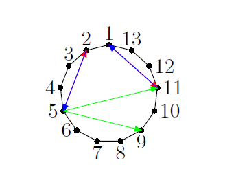
A 2-cluster tilting object in type F4F_{4} consists of two blue-red arrows in one of the graph in Figure 3 up to rotation and two green arrows in one of the graph in Figure 4 up to rotation such that the blue-red arrows do not cross green arrows. The mutation of an arrow is replacing it with another arrow such that the resulting graph satisfies the above conditions.

Refer to caption
Figure 3. All possible pairs of blue-red arrows appearing in a 22-cluster tilting object in 𝒞F42\mathcal{C}_{F_{4}}^{2} up to rotation.
Refer to caption
Figure 4. All possible pairs of green arrows appearing in a 22-cluster tilting object in 𝒞F42\mathcal{C}_{F_{4}}^{2} or 𝒞E62\mathcal{C}_{E_{6}}^{2} up to rotation.
Theorem 4.2.

A 22-cluster tilting object in type E6E_{6} consists of 66 arrows with colors red, blue, and green in a 1313-gon which satisfy the following properties.

  1. (1)

    The red arrows are of the form [i,i+8][i,i+8] or [i,i+10][i,i+10]. The blue arrows are of the form [i,i+3][i,i+3] or [i,i+5][i,i+5]. The green arrows are of the form [i,i+4][i,i+4] or [i,i+6][i,i+6].

  2. (2)

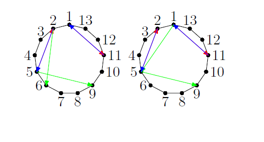
    If there are two or more red (resp. blue, resp. green) arrows, then any pair of red arrows are in one of the graphs in Figure 5 (resp. in the dual set of blue arrows with opposite orientation (not drawn), resp. Figure 4) up to rotation.

  3. (3)

    The blue and red arrows do not cross green arrows.

  4. (4)

    Any pair of blue and red arrows is in one of the graphs in Figure 6 up to rotation.

The mutation of an arrow is replacing it with another arrow such that the resulting graph satisfies the above conditions.

Refer to caption
Figure 5. All possible pairs of red arrows appearing in a 22-cluster tilting object in 𝒞E62\mathcal{C}_{E_{6}}^{2} up to rotation. Dually, one finds a lists of all possible pairs of blue arrows with opposite orientation (not drawn) appearing in a 22-cluster tilting object in 𝒞E62\mathcal{C}_{E_{6}}^{2} up to rotation.
Refer to caption
Figure 6. All possible pairs of one blue and one red arrows appearing in a 22-cluster tilting object in 𝒞E62\mathcal{C}_{E_{6}}^{2} up to rotation.
Refer to caption
Figure 7. Examples of 22-cluster tilting objects in 𝒞F42\mathcal{C}_{F_{4}}^{2}.
Example 4.3.

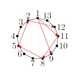
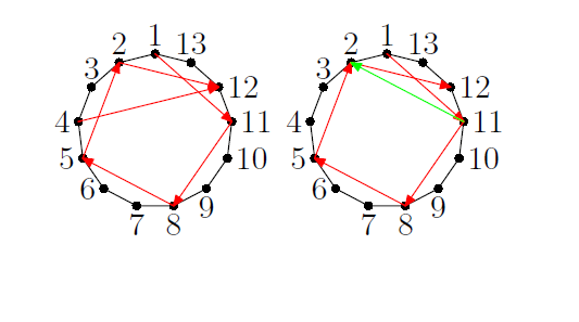
In Figure 8, the mutation of the arrow [5,11]P[5,11]_{P} in the left cluster gives the clusters on the right. Similarly, in Figure 9, the mutation of the arrow [1,9]R[1,9]_{R} in the left cluster gives the clusters on the right.

Refer to caption
Refer to caption
Figure 8. An example of mutations in 𝒞F42\mathcal{C}_{F_{4}}^{2}.
Refer to caption
Refer to caption
Figure 9. An example of mutations in 𝒞E62\mathcal{C}_{E_{6}}^{2}.

5. Cluster tilting objects in 𝒞F4\mathcal{C}_{F_{4}}, 𝒞E6\mathcal{C}_{E_{6}}, 𝒞E7\mathcal{C}_{E_{7}}, 𝒞E8\mathcal{C}_{E_{8}}

In this section we provide new descriptions of all cluster tilting objects in 𝒞F4\mathcal{C}_{F_{4}}, 𝒞E6\mathcal{C}_{E_{6}} extend the results obtained in [17]. These descriptions are also new for symmetric-clusters and clusters in ℂ⁡[Gr⁡(3,7)]\mathbb{C}[{\rm Gr}(3,7)], via [5, Prop.4.1] together with [23, Thm.5].

5.1. Cluster tilting objects in 𝒞F4\mathcal{C}_{F_{4}} and 𝒞E6\mathcal{C}_{E_{6}}

Theorem 5.1 and Theorem 5.3 are obtained by direct computations.

Theorem 5.1.

A cluster tilting object in type F4F_{4} consists of two blue-red arrows, as in Figure 10 up to rotation, and two green arrows, as in Figure 11 up to rotation. The arrows always combine, in such a way that the blue-red arrows do not cross green edges. However, blue-red arrows and green arrows can overlap.

The mutation of a blue-red arrow is to replace it with a blue-red arrow which satisfies the above conditions. The mutation of a green arrow is to replace it with a green arrow which satisfies the above conditions.

Refer to caption
Figure 10. All possible pairs of blue-red arrows in a cluster tiling object in 𝒞F4\mathcal{C}_{F_{4}} up to rotation.
Refer to caption
Figure 11. All possible pairs of green arrows in a cluster tiling object in 𝒞F4\mathcal{C}_{F_{4}} or 𝒞E6\mathcal{C}_{E_{6}} up to rotation.

Figure 12 are all cluster tilting objects (up to rotation) in type F4F_{4}.

Refer to caption
Figure 12. All cluster tilting objects in 𝒞F4\mathcal{C}_{F_{4}} up to rotation. All clusters have four diagonals, but some are overlapped.
Remark 5.2.

In Figure 12, the diagonals [1,6][1,6] and [4,6][4,6] in the last cluster have both a green arrow and a blue-red arrow. The diagonal [1,6][1,6] in the second cluster in the third line has both a green arrow and a blue-red arrow.

Theorem 5.3.

A cluster tilting object in type E6E_{6} consists of 66 arrows with colors red, blue, and green in a heptagon (the vertices are labelled clockwise) which satisfy the following properties.

  1. (1)

    The red edges are of the form [i,i+4]R[i,i+4]_{R} or [i,i+5]R[i,i+5]_{R}. The blue edges are of the form [i,i+2]B[i,i+2]_{B} or [i,i+3]B[i,i+3]_{B}. The green edges are of the form [i,i+2]P[i,i+2]_{P} or [i,i+3]P[i,i+3]_{P}.

  2. (2)

    If there are two or more red (resp. blue, green) arrows, then any pair of the red arrows is in one of the graph in Figure 13 (resp. in the dual set of blue arrows with opposite orientation, resp. Figure 11) up to rotation.

  3. (3)

    The blue and red arrows do not cross green arrows. A blue arrow can overlap with a green arrow and a red arrow can be the opposite arrow of a green arrow.

  4. (4)

    Any pair of blue and red arrows is in one of the graphs in Figure 14 up to rotation.

A mutation of an arrow in a cluster is replacing the diagonal with another arrow such that the resulting graph satisfies all the above conditions.

Refer to caption
Figure 13. All possible pairs of red arrows in a cluster tiling object in 𝒞E6\mathcal{C}_{E_{6}} up to rotation. Dually, one finds a lists of all possible pairs of blue arrows with opposite orientation (not drawn) appearing in a cluster tilting object in 𝒞E6\mathcal{C}_{E_{6}} up to rotation.
Refer to caption
Figure 14. All possible pairs of one blue and one red arrows in a cluster tiling object in 𝒞E6\mathcal{C}_{E_{6}} up to rotation.

In Figure 15 thirty examples of cluster tilting objects in 𝒞E6\mathcal{C}_{E_{6}}, are given. More cluster tilting objects can be deduced from them via π7\frac{\pi}{7}-rotations.

Refer to caption
Figure 15. Examples of clusters tilting objects in 𝒞E6\mathcal{C}_{E_{6}}.

5.2. Cluster tilting objects in 𝒞E7\mathcal{C}_{E_{7}} and 𝒞E8\mathcal{C}_{E_{8}}

The cases of types E7E_{7}, E8E_{8} are complicated and only some examples of cluster tilting objects and their mutations will be provided.

Example 5.4.

In Figure 17, the mutation of the arrow [9,5]R[9,5]_{R} in the left cluster gives the cluster on the right hand side. In Figure 17, the mutation of the arrow [3,5]R[3,5]_{R} in the left cluster gives the cluster on the right hand side.

Similarly, in Figure 19, the mutation of the arrow [9,13]R[9,13]_{R} in the left cluster gives the cluster on the right hand side. In Figure 19, the mutation of the arrow [10,12]R[10,12]_{R} in the left cluster gives the cluster on the right hand side.

Refer to caption
Figure 16. A mutation in 𝒞E7\mathcal{C}_{E_{7}}.
Refer to caption
Figure 17. A mutation in 𝒞E7\mathcal{C}_{E_{7}}.
Refer to caption
Figure 18. A mutation in 𝒞E8\mathcal{C}_{E_{8}}.
Refer to caption
Figure 19. A mutation in 𝒞E8\mathcal{C}_{E_{8}}.

6. Semi-standard Young tableaux and colored diagonals

In this section we link semi-standard Young tableaux to indecomposable objects of cluster categories of type E6,E7E_{6},E_{7} and E8E_{8}. To do so, we exploit the fact that indecomposable objects in these categories are in 1-1 correspondence with almost positive roots in the root system of the same type [5, Prop. 4.1] and hence with cluster variables in cluster algebras of the same type [9]. We then use the fact that every cluster variable in ℂ⁡[Gr⁡(n,m)]\mathbb{C}[{\rm Gr}(n,m)] corresponds to some tableau T∈SSYT⁡(n,[m])T\in{\rm SSYT}(n,[m]), as described in [6].

6.1. Tableaux and colored diagonals in 𝒞E6\mathcal{C}_{E_{6}}

Definition 6.1.

For T∈SSYT⁡(n,[m])T\in{\rm SSYT}(n,[m]) which corresponds to a cluster variable in the ring ℂ⁡[Gr⁡(n,m)],\mathbb{C}[\mathrm{Gr}(n,m)], we define τ⁡(T)\tau(T) to be the tableau in SSYT⁡(n,[m]){\rm SSYT}(n,[m]) such that τ⁡(ch⁡(T))\tau({\rm ch}(T)) is equal to ch⁡(τ⁡(T)){\rm ch}(\tau(T)) (possibly multiply by some frozen variables).

There are 2828 rank 11 cluster variables and 1414 rank 22 cluster variables in 𝒞E6\mathcal{C}_{E_{6}}.

In [23], Scott studied the correspondence between almost positive roots and cluster variables in type E6E_{6}, E8E_{8} explicitly. The cluster

𝐱=((346),(246),(124567),(123567),(147),(237)){\bf x}=\left(\left(\begin{array}[]{c}3\\ 4\\ 6\end{array}\right),\left(\begin{array}[]{c}2\\ 4\\ 6\end{array}\right),\left(\begin{array}[]{cc}1&2\\ 4&5\\ 6&7\end{array}\right),\left(\begin{array}[]{cc}1&2\\ 3&5\\ 6&7\end{array}\right),\left(\begin{array}[]{c}1\\ 4\\ 7\end{array}\right),\left(\begin{array}[]{c}2\\ 3\\ 7\end{array}\right)\right)

corresponds to the negative simple roots (−α6,−α5,−α4,−α3,−α2,−α1)(-\alpha_{6},-\alpha_{5},-\alpha_{4},-\alpha_{3},-\alpha_{2},-\alpha_{1}). We identify the cluster ([1,6]R,[1,5]R,[2,5]G,[5,1]B,[2,4]G,[6,1]B)([1,6]_{R},[1,5]_{R},[2,5]_{G},[5,1]_{B},[2,4]_{G},[6,1]_{B}) with 𝐱{\bf x}. In this way, the following two maps agree:

τ⁡(346)=(245)⟷τ⁡([1,6]R)=ρ⁡([7,5]R)=[5,7]B.\tau\left(\begin{array}[]{c}3\\ 4\\ 6\end{array}\right)=\left(\begin{array}[]{c}2\\ 4\\ 5\end{array}\right)\longleftrightarrow\tau([1,6]_{R})=\rho([7,5]_{R})=[5,7]_{B}.

In this way, one can associate to every colored diagonal a tableaux, by repeatedly applying the τ\tau-twist. Below, we describe this correspondence explicitly, see also Figures 1 and 21. We denote by TDT_{D} the tableau corresponding to a diagonal DD. We also write D=TDD=T_{D}.

For red diagonals, we have

[1,6]R=(346),[2,7]R=(157),[3,1]R=(267),[4,2]R=(134),[5,3]R=(235),\displaystyle[1,6]_{R}=\left(\begin{array}[]{c}3\\ 4\\ 6\end{array}\right),[2,7]_{R}=\left(\begin{array}[]{c}1\\ 5\\ 7\end{array}\right),[3,1]_{R}=\left(\begin{array}[]{c}2\\ 6\\ 7\end{array}\right),[4,2]_{R}=\left(\begin{array}[]{c}1\\ 3\\ 4\end{array}\right),[5,3]_{R}=\left(\begin{array}[]{c}2\\ 3\\ 5\end{array}\right),

[6,4]R=(467),[7,5]R=(156),[1,5]R=(246),[2,6]R=(134567),[3,7]R=(257),\displaystyle[6,4]_{R}=\left(\begin{array}[]{c}4\\ 6\\ 7\end{array}\right),[7,5]_{R}=\left(\begin{array}[]{c}1\\ 5\\ 6\end{array}\right),[1,5]_{R}=\left(\begin{array}[]{c}2\\ 4\\ 6\end{array}\right),[2,6]_{R}=\left(\begin{array}[]{cc}1&3\\ 4&5\\ 6&7\end{array}\right),[3,7]_{R}=\left(\begin{array}[]{c}2\\ 5\\ 7\end{array}\right),

[4,1]R=(132647),[5,2]R=(135),[6,3]R=(243657),[7,4]R=(146).\displaystyle[4,1]_{R}=\left(\begin{array}[]{cc}1&3\\ 2&6\\ 4&7\end{array}\right),[5,2]_{R}=\left(\begin{array}[]{c}1\\ 3\\ 5\end{array}\right),[6,3]_{R}=\left(\begin{array}[]{cc}2&4\\ 3&6\\ 5&7\end{array}\right),[7,4]_{R}=\left(\begin{array}[]{c}1\\ 4\\ 6\end{array}\right).

For blue diagonals, we have

[6,1]B=(237),[7,2]B=(124),[1,3]B=(356),[2,4]B=(457),[3,5]B=(126),\displaystyle[6,1]_{B}=\left(\begin{array}[]{cc}2\\ 3\\ 7\end{array}\right),[7,2]_{B}=\left(\begin{array}[]{c}1\\ 2\\ 4\end{array}\right),[1,3]_{B}=\left(\begin{array}[]{c}3\\ 5\\ 6\end{array}\right),[2,4]_{B}=\left(\begin{array}[]{c}4\\ 5\\ 7\end{array}\right),[3,5]_{B}=\left(\begin{array}[]{c}1\\ 2\\ 6\end{array}\right),

[4,6]B=(137),[5,7]B=(245),[5,1]B=(123567),[6,2]B=(247),[7,3]B=(132546),\displaystyle[4,6]_{B}=\left(\begin{array}[]{c}1\\ 3\\ 7\end{array}\right),[5,7]_{B}=\left(\begin{array}[]{c}2\\ 4\\ 5\end{array}\right),[5,1]_{B}=\left(\begin{array}[]{cc}1&2\\ 3&5\\ 6&7\end{array}\right),[6,2]_{B}=\left(\begin{array}[]{c}2\\ 4\\ 7\end{array}\right),[7,3]_{B}=\left(\begin{array}[]{cc}1&3\\ 2&5\\ 4&6\end{array}\right),

[1,4]B=(357),[2,5]B=(142657),[3,6]B=(136),[4,7]B=(123457).\displaystyle[1,4]_{B}=\left(\begin{array}[]{c}3\\ 5\\ 7\end{array}\right),[2,5]_{B}=\left(\begin{array}[]{cc}1&4\\ 2&6\\ 5&7\end{array}\right),[3,6]_{B}=\left(\begin{array}[]{c}1\\ 3\\ 6\end{array}\right),[4,7]_{B}=\left(\begin{array}[]{cc}1&2\\ 3&4\\ 5&7\end{array}\right).

For a sequence of numbers i1<…<imi_{1}<\ldots<i_{m}, we say that iji_{j} (j∈[m]j\in[m]) is the predecessor of ij+1i_{j+1} and ij+1i_{j+1} is the successor of iji_{j}, where we use the convention that im+1=i1i_{m+1}=i_{1}. Denote by s⁡(T)s(T) the sequence (from small to large) consisting of entries of a tableau TT.

For green diagonals, we have the following. For i∈{1,…,7}i\in\{1,\ldots,7\}, [i,i+2]G[i,i+2]_{G} corresponds to the one-column tableau with entries {a,b,c}\{a,b,c\}, where aa is the common element in both [i+2,i]R[i+2,i]_{R} and [i,i+2]B[i,i+2]_{B}, bb is the successor of aa in s⁡(T[i+2,i]R)s(T_{[i+2,i]_{R}}), and cc is the predecessor of aa in s⁡(T[i,i+2]B)s(T_{[i,i+2]_{B}}). For example, [2,4]G=(147)[2,4]_{G}=\left(\begin{array}[]{c}1\\ 4\\ 7\end{array}\right). For i∈[7]i\in[7], exactly one of [i+3,i]R[i+3,i]_{R} and [i,i+3]B[i,i+3]_{B} is a two column tableaux. Denote the tableau by (i1j1i2j2i3j3)\left(\begin{array}[]{cc}i_{1}&j_{1}\\ i_{2}&j_{2}\\ i_{3}&j_{3}\end{array}\right). Then [i,i+3]G=(i1i2j1i3j2j3)[i,i+3]_{G}=\left(\begin{array}[]{cc}i_{1}&i_{2}\\ j_{1}&i_{3}\\ j_{2}&j_{3}\end{array}\right).

A set of tableaux are called compatible if they are in the same cluster. The geometric model of cluster categories can be used to obtain results about the compatibility of tableaux. For example, in the first graph in Figure 15, the diagonals [1,6]R[1,6]_{R}, [1,5]R[1,5]_{R}, [7,5]R[7,5]_{R}, [5,1]B[5,1]_{B}, [1,4]G[1,4]_{G}, [2,4]G[2,4]_{G} form a cluster. Therefore the corresponding tableaux

(346),(246),(156),(123567),(123467),(147),\displaystyle\left(\begin{array}[]{c}3\\ 4\\ 6\end{array}\right),\left(\begin{array}[]{c}2\\ 4\\ 6\end{array}\right),\left(\begin{array}[]{c}1\\ 5\\ 6\end{array}\right),\left(\begin{array}[]{cc}1&2\\ 3&5\\ 6&7\end{array}\right),\left(\begin{array}[]{cc}1&2\\ 3&4\\ 6&7\end{array}\right),\left(\begin{array}[]{c}1\\ 4\\ 7\end{array}\right),

are compatible.

6.2. Tableaux and colored diagonals in 𝒞E7\mathcal{C}_{E_{7}}

In order to have a correspondence between oriented diagonals and tableaux in the case of E7E_{7}, we froze P167P_{167} in the initial quiver in Figure 20. Note that the Plücker coordinate Pi1,…,ikP_{i_{1},\ldots,i_{k}} corresponds to the one column tableau with entries i1,…,iki_{1},\ldots,i_{k}.

P123P_{123}P124P_{124}P125P_{125}P126P_{126}P127P_{127}P128P_{128}P134P_{134}P145P_{145}P156P_{156}P167P_{167}P178P_{178}P234P_{234}P345P_{345}P456P_{456}P567P_{567}P678P_{678}
Figure 20. The initial cluster for 𝒞E7\mathcal{C}_{E_{7}}.

There are 3333 rank 11 cluster variables, 2929 rank 22 cluster variables, and 88 rank 33 cluster variables in 𝒞E7\mathcal{C}_{E_{7}}. They can be obtained from the initial quiver in Figure 20 by mutations.

We identify the cluster ([10,6]R,[1,6]R,[1,5]R,[2,5]G,[5,1]B,[2,4]G,[6,1]B)([10,6]_{R},[1,6]_{R},[1,5]_{R},[2,5]_{G},[5,1]_{B},[2,4]_{G},[6,1]_{B}) with the cluster

𝐱=((157),(123578),(123345678),(123445678),(124568),(247),(256)).\displaystyle{\bf x}=\left(\left(\begin{array}[]{c}1\\ 5\\ 7\end{array}\right),\left(\begin{array}[]{cc}1&2\\ 3&5\\ 7&8\end{array}\right),\left(\begin{array}[]{ccc}1&2&3\\ 3&4&5\\ 6&7&8\end{array}\right),\left(\begin{array}[]{ccc}1&2&3\\ 4&4&5\\ 6&7&8\end{array}\right),\left(\begin{array}[]{cc}1&2\\ 4&5\\ 6&8\end{array}\right),\left(\begin{array}[]{c}2\\ 4\\ 7\end{array}\right),\left(\begin{array}[]{c}2\\ 5\\ 6\end{array}\right)\right).

The correspondence between tableaux and diagonals can be deduced by combining the Auslander–Reiten quiver of 𝒞E7\mathcal{C}_{E_{7}} with the stable translations graph given in Figure 22 and Figure 23. The first two slices from the Auslander–Reiten quiver of 𝒞E7\mathcal{C}_{E_{7}} are illustrated on the left in Figure 2.

6.3. Tableaux and colored diagonals in 𝒞E8\mathcal{C}_{E_{8}}

There are 4848 rank 11 cluster variables, 5656 rank 22 cluster variables, and 2424 rank 33 cluster variables in 𝒞E8\mathcal{C}_{E_{8}}.

In [23], Scott verified that in type E8E_{8}, the cluster

𝐱=((457),(357),(135678),(113256478),(123256478),(234678),(258),(348))\displaystyle{\bf x}=\left(\left(\begin{array}[]{c}4\\ 5\\ 7\end{array}\right),\left(\begin{array}[]{c}3\\ 5\\ 7\end{array}\right),\left(\begin{array}[]{cc}1&3\\ 5&6\\ 7&8\end{array}\right),\left(\begin{array}[]{ccc}1&1&3\\ 2&5&6\\ 4&7&8\end{array}\right),\left(\begin{array}[]{ccc}1&2&3\\ 2&5&6\\ 4&7&8\end{array}\right),\left(\begin{array}[]{cc}2&3\\ 4&6\\ 7&8\end{array}\right),\left(\begin{array}[]{c}2\\ 5\\ 8\end{array}\right),\left(\begin{array}[]{c}3\\ 4\\ 8\end{array}\right)\right)

correspond to the negative simple roots (−α8,−α7,−α6,−α5,−α4,−α3,−α2,−α1)(-\alpha_{8},-\alpha_{7},-\alpha_{6},-\alpha_{5},-\alpha_{4},-\alpha_{3},-\alpha_{2},-\alpha_{1}). We identify the cluster ([16,7]R,[16,6]R,[1,6]R,[1,5]R,[2,5]G,[5,1]B,[2,4]G,[6,1]B)([16,7]_{R},[16,6]_{R},[1,6]_{R},[1,5]_{R},[2,5]_{G},[5,1]_{B},[2,4]_{G},[6,1]_{B}) with 𝐱{\bf x}.

The correspondence between tableaux and diagonals can be deduced by combining the Auslander–Reiten quiver of 𝒞E8\mathcal{C}_{E_{8}}, with initial slices given as in Figure 2, with the stable translations graph given in Figure 24, Figure 25 and Figure 26.

Proposition 6.2.

In the Auslander–Reiten quivers of 𝒞E6\mathcal{C}_{E_{6}}, 𝒞E7\mathcal{C}_{E_{7}}, 𝒞E8\mathcal{C}_{E_{8}}, for every mesh of the form:

T1\textstyle{T_{1}\ignorespaces\ignorespaces\ignorespaces\ignorespaces}S1\textstyle{S_{1}\ignorespaces\ignorespaces\ignorespaces\ignorespaces\ignorespaces\ignorespaces\ignorespaces\ignorespaces\ignorespaces\ignorespaces\ignorespaces\ignorespaces}⋮\textstyle{\ignorespaces\ignorespaces\ignorespaces\ignorespaces\vdots}S2\textstyle{S_{2}}Tk\textstyle{T_{k}\ignorespaces\ignorespaces\ignorespaces\ignorespaces}

where k∈{2,3}k\in\{2,3\}, we have that S1∪S2=T1∪⋯∪TkS_{1}\cup S_{2}=T_{1}\cup\cdots\cup T_{k} up to permutation of entries in S1∪S2S_{1}\cup S_{2}.

Proof.

The proposition follows from the explicit descriptions of the Auslander–Reiten quivers of 𝒞E6\mathcal{C}_{E_{6}}, 𝒞E7\mathcal{C}_{E_{7}}, 𝒞E8\mathcal{C}_{E_{8}}. ∎

(346)\left(\begin{array}[]{c}3\\ 4\\ 6\end{array}\right)(157)\left(\begin{array}[]{c}1\\ 5\\ 7\end{array}\right)(267)\left(\begin{array}[]{c}2\\ 6\\ 7\end{array}\right)(134)\left(\begin{array}[]{c}1\\ 3\\ 4\end{array}\right)(235)\left(\begin{array}[]{c}2\\ 3\\ 5\end{array}\right)(467)\left(\begin{array}[]{c}4\\ 6\\ 7\end{array}\right)(156)\left(\begin{array}[]{c}1\\ 5\\ 6\end{array}\right)(237)\left(\begin{array}[]{c}2\\ 3\\ 7\end{array}\right)(246)\left(\begin{array}[]{c}2\\ 4\\ 6\end{array}\right)(134567)\left(\begin{array}[]{cc}1&3\\ 4&5\\ 6&7\end{array}\right)(257)\left(\begin{array}[]{c}2\\ 5\\ 7\end{array}\right)(132647)\left(\begin{array}[]{cc}1&3\\ 2&6\\ 4&7\end{array}\right)(135)\left(\begin{array}[]{c}1\\ 3\\ 5\end{array}\right)(243657)\left(\begin{array}[]{cc}2&4\\ 3&6\\ 5&7\end{array}\right)(146)\left(\begin{array}[]{c}1\\ 4\\ 6\end{array}\right)(123567)\left(\begin{array}[]{cc}1&2\\ 3&5\\ 6&7\end{array}\right)(147)\left(\begin{array}[]{c}1\\ 4\\ 7\end{array}\right)(124567)\left(\begin{array}[]{cc}1&2\\ 4&5\\ 6&7\end{array}\right)(256)\left(\begin{array}[]{c}2\\ 5\\ 6\end{array}\right)(234567)\left(\begin{array}[]{cc}2&3\\ 4&5\\ 6&7\end{array}\right)(347)\left(\begin{array}[]{c}3\\ 4\\ 7\end{array}\right)(132547)\left(\begin{array}[]{cc}1&3\\ 2&5\\ 4&7\end{array}\right)(125)\left(\begin{array}[]{c}1\\ 2\\ 5\end{array}\right)(132657)\left(\begin{array}[]{cc}1&3\\ 2&6\\ 5&7\end{array}\right)(367)\left(\begin{array}[]{c}3\\ 6\\ 7\end{array}\right)(143657)\left(\begin{array}[]{cc}1&4\\ 3&6\\ 5&7\end{array}\right)(145)\left(\begin{array}[]{c}1\\ 4\\ 5\end{array}\right)(123456)\left(\begin{array}[]{cc}1&2\\ 3&4\\ 5&6\end{array}\right)(236)\left(\begin{array}[]{c}2\\ 3\\ 6\end{array}\right)(123467)\left(\begin{array}[]{cc}1&2\\ 3&4\\ 6&7\end{array}\right)(147)\left(\begin{array}[]{c}1\\ 4\\ 7\end{array}\right)(124567)\left(\begin{array}[]{cc}1&2\\ 4&5\\ 6&7\end{array}\right)(123567)\left(\begin{array}[]{cc}1&2\\ 3&5\\ 6&7\end{array}\right)(247)\left(\begin{array}[]{c}2\\ 4\\ 7\end{array}\right)(132546)\left(\begin{array}[]{cc}1&3\\ 2&5\\ 4&6\end{array}\right)(357)\left(\begin{array}[]{c}3\\ 5\\ 7\end{array}\right)(142657)\left(\begin{array}[]{cc}1&4\\ 2&6\\ 5&7\end{array}\right)(136)\left(\begin{array}[]{c}1\\ 3\\ 6\end{array}\right)(123457)\left(\begin{array}[]{cc}1&2\\ 3&4\\ 5&7\end{array}\right)(246)\left(\begin{array}[]{c}2\\ 4\\ 6\end{array}\right)(237)\left(\begin{array}[]{c}2\\ 3\\ 7\end{array}\right)(124)\left(\begin{array}[]{c}1\\ 2\\ 4\end{array}\right)(356)\left(\begin{array}[]{c}3\\ 5\\ 6\end{array}\right)(457)\left(\begin{array}[]{c}4\\ 5\\ 7\end{array}\right)(126)\left(\begin{array}[]{c}1\\ 2\\ 6\end{array}\right)(137)\left(\begin{array}[]{c}1\\ 3\\ 7\end{array}\right)(245)\left(\begin{array}[]{c}2\\ 4\\ 5\end{array}\right)(346)\left(\begin{array}[]{c}3\\ 4\\ 6\end{array}\right)

Figure 21. Auslander–Reiten quiver of 𝒞E6\mathcal{C}_{E_{6}} with vertices labelled by tableaux.

(157)\left(\begin{array}[]{c}1\\ 5\\ 7\end{array}\right)(123678)\left(\begin{array}[]{cc}1&2\\ 3&6\\ 7&8\end{array}\right)(124)\left(\begin{array}[]{c}1\\ 2\\ 4\end{array}\right)(356)\left(\begin{array}[]{c}3\\ 5\\ 6\end{array}\right)(457)\left(\begin{array}[]{c}4\\ 5\\ 7\end{array}\right)(168)\left(\begin{array}[]{c}1\\ 6\\ 8\end{array}\right)(123578)\left(\begin{array}[]{cc}1&2\\ 3&5\\ 7&8\end{array}\right)(124678)\left(\begin{array}[]{cc}1&2\\ 4&6\\ 7&8\end{array}\right)(132546)\left(\begin{array}[]{cc}1&3\\ 2&5\\ 4&6\end{array}\right)(357)\left(\begin{array}[]{c}3\\ 5\\ 7\end{array}\right)(145678)\left(\begin{array}[]{cc}1&4\\ 5&6\\ 7&8\end{array}\right)(123345678)\left(\begin{array}[]{ccc}1&2&3\\ 3&4&5\\ 6&7&8\end{array}\right)(124578)\left(\begin{array}[]{cc}1&2\\ 4&5\\ 7&8\end{array}\right)(123456678)\left(\begin{array}[]{ccc}1&2&3\\ 4&5&6\\ 6&7&8\end{array}\right)(132547)\left(\begin{array}[]{cc}1&3\\ 2&5\\ 4&7\end{array}\right)(135678)\left(\begin{array}[]{cc}1&3\\ 5&6\\ 7&8\end{array}\right)(142657)\left(\begin{array}[]{cc}1&4\\ 2&6\\ 5&7\end{array}\right)(247)\left(\begin{array}[]{c}2\\ 4\\ 7\end{array}\right)(123445678)\left(\begin{array}[]{ccc}1&2&3\\ 4&4&5\\ 6&7&8\end{array}\right)(134568)\left(\begin{array}[]{cc}1&3\\ 4&5\\ 6&8\end{array}\right)(123455678)\left(\begin{array}[]{ccc}1&2&3\\ 4&5&5\\ 6&7&8\end{array}\right)(257)\left(\begin{array}[]{c}2\\ 5\\ 7\end{array}\right)(123456778)\left(\begin{array}[]{ccc}1&2&3\\ 4&5&6\\ 7&7&8\end{array}\right)(134678)\left(\begin{array}[]{cc}1&3\\ 4&6\\ 7&8\end{array}\right)(113256478)\left(\begin{array}[]{ccc}1&1&3\\ 2&5&6\\ 4&7&8\end{array}\right)(125)\left(\begin{array}[]{c}1\\ 2\\ 5\end{array}\right)(132657)\left(\begin{array}[]{cc}1&3\\ 2&6\\ 5&7\end{array}\right)(367)\left(\begin{array}[]{c}3\\ 6\\ 7\end{array}\right)(124568)\left(\begin{array}[]{cc}1&2\\ 4&5\\ 6&8\end{array}\right)(234567)\left(\begin{array}[]{cc}2&3\\ 4&5\\ 6&7\end{array}\right)(134578)\left(\begin{array}[]{cc}1&3\\ 4&5\\ 7&8\end{array}\right)(125678)\left(\begin{array}[]{cc}1&2\\ 5&6\\ 7&8\end{array}\right)(132647)\left(\begin{array}[]{cc}1&3\\ 2&6\\ 4&7\end{array}\right)(135)\left(\begin{array}[]{c}1\\ 3\\ 5\end{array}\right)(256)\left(\begin{array}[]{c}2\\ 5\\ 6\end{array}\right)(347)\left(\begin{array}[]{c}3\\ 4\\ 7\end{array}\right)(158)\left(\begin{array}[]{c}1\\ 5\\ 8\end{array}\right)(267)\left(\begin{array}[]{c}2\\ 6\\ 7\end{array}\right)(134)\left(\begin{array}[]{c}1\\ 3\\ 4\end{array}\right)

Figure 22. Auslander–Reiten quiver of 𝒞E7\mathcal{C}_{E_{7}} with vertices labelled by tableaux, Part 1.

(168)\left(\begin{array}[]{c}1\\ 6\\ 8\end{array}\right)(127)\left(\begin{array}[]{c}1\\ 2\\ 7\end{array}\right)(138)\left(\begin{array}[]{c}1\\ 3\\ 8\end{array}\right)(245)\left(\begin{array}[]{c}2\\ 4\\ 5\end{array}\right)(346)\left(\begin{array}[]{c}3\\ 4\\ 6\end{array}\right)(157)\left(\begin{array}[]{c}1\\ 5\\ 7\end{array}\right)(126)\left(\begin{array}[]{c}1\\ 2\\ 6\end{array}\right)(137)\left(\begin{array}[]{c}1\\ 3\\ 7\end{array}\right)(123458)\left(\begin{array}[]{cc}1&2\\ 3&4\\ 5&8\end{array}\right)(246)\left(\begin{array}[]{c}2\\ 4\\ 6\end{array}\right)(134567)\left(\begin{array}[]{cc}1&3\\ 4&5\\ 6&7\end{array}\right)(142657)\left(\begin{array}[]{cc}1&4\\ 2&6\\ 5&7\end{array}\right)(136)\left(\begin{array}[]{c}1\\ 3\\ 6\end{array}\right)(123457)\left(\begin{array}[]{cc}1&2\\ 3&4\\ 5&7\end{array}\right)(123468)\left(\begin{array}[]{cc}1&2\\ 3&4\\ 6&8\end{array}\right)(124567)\left(\begin{array}[]{cc}1&2\\ 4&5\\ 6&7\end{array}\right)(123345678)\left(\begin{array}[]{ccc}1&2&3\\ 3&4&5\\ 6&7&8\end{array}\right)(367)\left(\begin{array}[]{c}3\\ 6\\ 7\end{array}\right)(143657)\left(\begin{array}[]{cc}1&4\\ 3&6\\ 5&7\end{array}\right)(145)\left(\begin{array}[]{c}1\\ 4\\ 5\end{array}\right)(123456)\left(\begin{array}[]{cc}1&2\\ 3&4\\ 5&6\end{array}\right)(236)\left(\begin{array}[]{c}2\\ 3\\ 6\end{array}\right)(123467)\left(\begin{array}[]{cc}1&2\\ 3&4\\ 6&7\end{array}\right)(147)\left(\begin{array}[]{c}1\\ 4\\ 7\end{array}\right)(112345678)\left(\begin{array}[]{ccc}1&1&2\\ 3&4&5\\ 6&7&8\end{array}\right)(123568)\left(\begin{array}[]{cc}1&2\\ 3&5\\ 6&8\end{array}\right)(122345678)\left(\begin{array}[]{ccc}1&2&2\\ 3&4&5\\ 6&7&8\end{array}\right)(247)\left(\begin{array}[]{c}2\\ 4\\ 7\end{array}\right)(135)\left(\begin{array}[]{c}1\\ 3\\ 5\end{array}\right)(243657)\left(\begin{array}[]{cc}2&4\\ 3&6\\ 5&7\end{array}\right)(146)\left(\begin{array}[]{c}1\\ 4\\ 6\end{array}\right)(123567)\left(\begin{array}[]{cc}1&2\\ 3&5\\ 6&7\end{array}\right)(123478)\left(\begin{array}[]{cc}1&2\\ 3&4\\ 7&8\end{array}\right)(124568)\left(\begin{array}[]{cc}1&2\\ 4&5\\ 6&8\end{array}\right)(235)\left(\begin{array}[]{c}2\\ 3\\ 5\end{array}\right)(467)\left(\begin{array}[]{c}4\\ 6\\ 7\end{array}\right)(156)\left(\begin{array}[]{c}1\\ 5\\ 6\end{array}\right)(237)\left(\begin{array}[]{c}2\\ 3\\ 7\end{array}\right)(148)\left(\begin{array}[]{c}1\\ 4\\ 8\end{array}\right)

Figure 23. Auslander–Reiten quiver of 𝒞E7\mathcal{C}_{E_{7}} with vertices labelled by tableaux, Part 2.

(457)\left(\begin{array}[]{c}4\\ 5\\ 7\end{array}\right)(168)\left(\begin{array}[]{c}1\\ 6\\ 8\end{array}\right)(278)\left(\begin{array}[]{c}2\\ 7\\ 8\end{array}\right)(134)\left(\begin{array}[]{c}1\\ 3\\ 4\end{array}\right)(235)\left(\begin{array}[]{c}2\\ 3\\ 5\end{array}\right)(467)\left(\begin{array}[]{c}4\\ 6\\ 7\end{array}\right)(357)\left(\begin{array}[]{c}3\\ 5\\ 7\end{array}\right)(145678)\left(\begin{array}[]{cc}1&4\\ 5&6\\ 7&8\end{array}\right)(268)\left(\begin{array}[]{c}2\\ 6\\ 8\end{array}\right)(132748)\left(\begin{array}[]{cc}1&3\\ 2&7\\ 4&8\end{array}\right)(135)\left(\begin{array}[]{c}1\\ 3\\ 5\end{array}\right)(243657)\left(\begin{array}[]{cc}2&4\\ 3&6\\ 5&7\end{array}\right)(468)\left(\begin{array}[]{c}4\\ 6\\ 8\end{array}\right)(135678)\left(\begin{array}[]{cc}1&3\\ 5&6\\ 7&8\end{array}\right)(245678)\left(\begin{array}[]{cc}2&4\\ 5&6\\ 7&8\end{array}\right)(132648)\left(\begin{array}[]{cc}1&3\\ 2&6\\ 4&8\end{array}\right)(132758)\left(\begin{array}[]{cc}1&3\\ 2&7\\ 5&8\end{array}\right)(143657)\left(\begin{array}[]{cc}1&4\\ 3&6\\ 5&7\end{array}\right)(243658)\left(\begin{array}[]{cc}2&4\\ 3&6\\ 5&8\end{array}\right)(113256478)\left(\begin{array}[]{ccc}1&1&3\\ 2&5&6\\ 4&7&8\end{array}\right)(235678)\left(\begin{array}[]{cc}2&3\\ 5&6\\ 7&8\end{array}\right)(134256478)\left(\begin{array}[]{ccc}1&3&4\\ 2&5&6\\ 4&7&8\end{array}\right)(132658)\left(\begin{array}[]{cc}1&3\\ 2&6\\ 5&8\end{array}\right)(134267578)\left(\begin{array}[]{ccc}1&3&4\\ 2&6&7\\ 5&7&8\end{array}\right)(143658)\left(\begin{array}[]{cc}1&4\\ 3&6\\ 5&8\end{array}\right)(124237568)\left(\begin{array}[]{ccc}1&2&4\\ 2&3&7\\ 5&6&8\end{array}\right)(258)\left(\begin{array}[]{c}2\\ 5\\ 8\end{array}\right)(123256478)\left(\begin{array}[]{ccc}1&2&3\\ 2&5&6\\ 4&7&8\end{array}\right)(132647)\left(\begin{array}[]{cc}1&3\\ 2&6\\ 4&7\end{array}\right)(133256478)\left(\begin{array}[]{ccc}1&3&3\\ 2&5&6\\ 4&7&8\end{array}\right)(358)\left(\begin{array}[]{c}3\\ 5\\ 8\end{array}\right)(134256578)\left(\begin{array}[]{ccc}1&3&4\\ 2&5&6\\ 5&7&8\end{array}\right)(142657)\left(\begin{array}[]{cc}1&4\\ 2&6\\ 5&7\end{array}\right)(134266578)\left(\begin{array}[]{ccc}1&3&4\\ 2&6&6\\ 5&7&8\end{array}\right)(368)\left(\begin{array}[]{c}3\\ 6\\ 8\end{array}\right)(134267588)\left(\begin{array}[]{ccc}1&3&4\\ 2&6&7\\ 5&8&8\end{array}\right)(142758)\left(\begin{array}[]{cc}1&4\\ 2&7\\ 5&8\end{array}\right)(114237568)\left(\begin{array}[]{ccc}1&1&4\\ 2&3&7\\ 5&6&8\end{array}\right)(136)\left(\begin{array}[]{c}1\\ 3\\ 6\end{array}\right)(234678)\left(\begin{array}[]{cc}2&3\\ 4&6\\ 7&8\end{array}\right)(132548)\left(\begin{array}[]{cc}1&3\\ 2&5\\ 4&8\end{array}\right)(132657)\left(\begin{array}[]{cc}1&3\\ 2&6\\ 5&7\end{array}\right)(345678)\left(\begin{array}[]{cc}3&4\\ 5&6\\ 7&8\end{array}\right)(142658)\left(\begin{array}[]{cc}1&4\\ 2&6\\ 5&8\end{array}\right)(132768)\left(\begin{array}[]{cc}1&3\\ 2&7\\ 6&8\end{array}\right)(143758)\left(\begin{array}[]{cc}1&4\\ 3&7\\ 5&8\end{array}\right)(348)\left(\begin{array}[]{c}3\\ 4\\ 8\end{array}\right)(125)\left(\begin{array}[]{c}1\\ 2\\ 5\end{array}\right)(367)\left(\begin{array}[]{c}3\\ 6\\ 7\end{array}\right)(458)\left(\begin{array}[]{c}4\\ 5\\ 8\end{array}\right)(126)\left(\begin{array}[]{c}1\\ 2\\ 6\end{array}\right)(378)\left(\begin{array}[]{c}3\\ 7\\ 8\end{array}\right)

Figure 24. Auslander–Reiten quiver of 𝒞E8\mathcal{C}_{E_{8}} with vertices labelled by tableaux, Part 1.

(568)\left(\begin{array}[]{c}5\\ 6\\ 8\end{array}\right)(127)\left(\begin{array}[]{c}1\\ 2\\ 7\end{array}\right)(138)\left(\begin{array}[]{c}1\\ 3\\ 8\end{array}\right)(245)\left(\begin{array}[]{c}2\\ 4\\ 5\end{array}\right)(346)\left(\begin{array}[]{c}3\\ 4\\ 6\end{array}\right)(468)\left(\begin{array}[]{c}4\\ 6\\ 8\end{array}\right)(152768)\left(\begin{array}[]{cc}1&5\\ 2&7\\ 6&8\end{array}\right)(137)\left(\begin{array}[]{c}1\\ 3\\ 7\end{array}\right)(123458)\left(\begin{array}[]{cc}1&2\\ 3&4\\ 5&8\end{array}\right)(246)\left(\begin{array}[]{c}2\\ 4\\ 6\end{array}\right)(354768)\left(\begin{array}[]{cc}3&5\\ 4&7\\ 6&8\end{array}\right)(142768)\left(\begin{array}[]{cc}1&4\\ 2&7\\ 6&8\end{array}\right)(153768)\left(\begin{array}[]{cc}1&5\\ 3&7\\ 6&8\end{array}\right)(123457)\left(\begin{array}[]{cc}1&2\\ 3&4\\ 5&7\end{array}\right)(123468)\left(\begin{array}[]{cc}1&2\\ 3&4\\ 6&8\end{array}\right)(254768)\left(\begin{array}[]{cc}2&5\\ 4&7\\ 6&8\end{array}\right)(124237568)\left(\begin{array}[]{ccc}1&2&4\\ 2&3&7\\ 5&6&8\end{array}\right)(143768)\left(\begin{array}[]{cc}1&4\\ 3&7\\ 6&8\end{array}\right)(125347568)\left(\begin{array}[]{ccc}1&2&5\\ 3&4&7\\ 5&6&8\end{array}\right)(123467)\left(\begin{array}[]{cc}1&2\\ 3&4\\ 6&7\end{array}\right)(125347688)\left(\begin{array}[]{ccc}1&2&5\\ 3&4&7\\ 6&8&8\end{array}\right)(124567)\left(\begin{array}[]{cc}1&2\\ 4&5\\ 6&7\end{array}\right)(136)\left(\begin{array}[]{c}1\\ 3\\ 6\end{array}\right)(124337568)\left(\begin{array}[]{ccc}1&2&4\\ 3&3&7\\ 5&6&8\end{array}\right)(243758)\left(\begin{array}[]{cc}2&4\\ 3&7\\ 5&8\end{array}\right)(124347568)\left(\begin{array}[]{ccc}1&2&4\\ 3&4&7\\ 5&6&8\end{array}\right)(146)\left(\begin{array}[]{c}1\\ 4\\ 6\end{array}\right)(125347668)\left(\begin{array}[]{ccc}1&2&5\\ 3&4&7\\ 6&6&8\end{array}\right)(253768)\left(\begin{array}[]{cc}2&5\\ 3&7\\ 6&8\end{array}\right)(125347678)\left(\begin{array}[]{ccc}1&2&5\\ 3&4&7\\ 6&7&8\end{array}\right)(147)\left(\begin{array}[]{c}1\\ 4\\ 7\end{array}\right)(112345678)\left(\begin{array}[]{ccc}1&1&2\\ 3&4&5\\ 6&7&8\end{array}\right)(123568)\left(\begin{array}[]{cc}1&2\\ 3&5\\ 6&8\end{array}\right)(143758)\left(\begin{array}[]{cc}1&4\\ 3&7\\ 5&8\end{array}\right)(123456)\left(\begin{array}[]{cc}1&2\\ 3&4\\ 5&6\end{array}\right)(243768)\left(\begin{array}[]{cc}2&4\\ 3&7\\ 6&8\end{array}\right)(154768)\left(\begin{array}[]{cc}1&5\\ 4&7\\ 6&8\end{array}\right)(123567)\left(\begin{array}[]{cc}1&2\\ 3&5\\ 6&7\end{array}\right)(123478)\left(\begin{array}[]{cc}1&2\\ 3&4\\ 7&8\end{array}\right)(145)\left(\begin{array}[]{c}1\\ 4\\ 5\end{array}\right)(236)\left(\begin{array}[]{c}2\\ 3\\ 6\end{array}\right)(478)\left(\begin{array}[]{c}4\\ 7\\ 8\end{array}\right)(156)\left(\begin{array}[]{c}1\\ 5\\ 6\end{array}\right)(237)\left(\begin{array}[]{c}2\\ 3\\ 7\end{array}\right)

Figure 25. Auslander–Reiten quiver of 𝒞E8\mathcal{C}_{E_{8}} with vertices labelled by tableaux, Part 2.

(578)\left(\begin{array}[]{c}5\\ 7\\ 8\end{array}\right)(167)\left(\begin{array}[]{c}1\\ 6\\ 7\end{array}\right)(238)\left(\begin{array}[]{c}2\\ 3\\ 8\end{array}\right)(124)\left(\begin{array}[]{c}1\\ 2\\ 4\end{array}\right)(356)\left(\begin{array}[]{c}3\\ 5\\ 6\end{array}\right)(354768)\left(\begin{array}[]{cc}3&5\\ 4&7\\ 6&8\end{array}\right)(157)\left(\begin{array}[]{c}1\\ 5\\ 7\end{array}\right)(123678)\left(\begin{array}[]{cc}1&2\\ 3&6\\ 7&8\end{array}\right)(248)\left(\begin{array}[]{c}2\\ 4\\ 8\end{array}\right)(132546)\left(\begin{array}[]{cc}1&3\\ 2&5\\ 4&6\end{array}\right)(357)\left(\begin{array}[]{c}3\\ 5\\ 7\end{array}\right)(134567)\left(\begin{array}[]{cc}1&3\\ 4&5\\ 6&7\end{array}\right)(123578)\left(\begin{array}[]{cc}1&2\\ 3&5\\ 7&8\end{array}\right)(124678)\left(\begin{array}[]{cc}1&2\\ 4&6\\ 7&8\end{array}\right)(234568)\left(\begin{array}[]{cc}2&3\\ 4&5\\ 6&8\end{array}\right)(132547)\left(\begin{array}[]{cc}1&3\\ 2&5\\ 4&7\end{array}\right)(124567)\left(\begin{array}[]{cc}1&2\\ 4&5\\ 6&7\end{array}\right)(123345678)\left(\begin{array}[]{ccc}1&2&3\\ 3&4&5\\ 6&7&8\end{array}\right)(124578)\left(\begin{array}[]{cc}1&2\\ 4&5\\ 7&8\end{array}\right)(123456678)\left(\begin{array}[]{ccc}1&2&3\\ 4&5&6\\ 6&7&8\end{array}\right)(234578)\left(\begin{array}[]{cc}2&3\\ 4&5\\ 7&8\end{array}\right)(113256478)\left(\begin{array}[]{ccc}1&1&3\\ 2&5&6\\ 4&7&8\end{array}\right)(123568)\left(\begin{array}[]{cc}1&2\\ 3&5\\ 6&8\end{array}\right)(122345678)\left(\begin{array}[]{ccc}1&2&2\\ 3&4&5\\ 6&7&8\end{array}\right)(247)\left(\begin{array}[]{c}2\\ 4\\ 7\end{array}\right)(123445678)\left(\begin{array}[]{ccc}1&2&3\\ 4&4&5\\ 6&7&8\end{array}\right)(134568)\left(\begin{array}[]{cc}1&3\\ 4&5\\ 6&8\end{array}\right)(123455678)\left(\begin{array}[]{ccc}1&2&3\\ 4&5&5\\ 6&7&8\end{array}\right)(257)\left(\begin{array}[]{c}2\\ 5\\ 7\end{array}\right)(123456778)\left(\begin{array}[]{ccc}1&2&3\\ 4&5&6\\ 7&7&8\end{array}\right)(134678)\left(\begin{array}[]{cc}1&3\\ 4&6\\ 7&8\end{array}\right)(123456788)\left(\begin{array}[]{ccc}1&2&3\\ 4&5&6\\ 7&8&8\end{array}\right)(258)\left(\begin{array}[]{c}2\\ 5\\ 8\end{array}\right)(123478)\left(\begin{array}[]{cc}1&2\\ 3&4\\ 7&8\end{array}\right)(124568)\left(\begin{array}[]{cc}1&2\\ 4&5\\ 6&8\end{array}\right)(234567)\left(\begin{array}[]{cc}2&3\\ 4&5\\ 6&7\end{array}\right)(134578)\left(\begin{array}[]{cc}1&3\\ 4&5\\ 7&8\end{array}\right)(125678)\left(\begin{array}[]{cc}1&2\\ 5&6\\ 7&8\end{array}\right)(234678)\left(\begin{array}[]{cc}2&3\\ 4&6\\ 7&8\end{array}\right)(148)\left(\begin{array}[]{c}1\\ 4\\ 8\end{array}\right)(256)\left(\begin{array}[]{c}2\\ 5\\ 6\end{array}\right)(347)\left(\begin{array}[]{c}3\\ 4\\ 7\end{array}\right)(158)\left(\begin{array}[]{c}1\\ 5\\ 8\end{array}\right)(267)\left(\begin{array}[]{c}2\\ 6\\ 7\end{array}\right)

Figure 26. Auslander–Reiten quiver of 𝒞E8\mathcal{C}_{E_{8}} with vertices labelled by tableaux, Part 3.

References

  • [1] A. Berenstein, S. Fomin, and A. Zelevinsky, Parametrizations of canonical bases and totally positive matrices. Adv. Math. 122 (1996), no. 1, 49–149.
  • [2] A. Berenstein and A. Zelevinsky, Total positivity in Schubert varieties. Comm. Math. Helv. 72 (1997), no. 1, 128–166.
  • [3] K. Baur and R. J. Marsh. A geometric description of mm-cluster categories. Trans. Amer. Math. Soc. 360 (2008), no. 11, 5789–5803.
  • [4] K. Baur and R. J. Marsh. A Geometric Description of the mm-cluster Categories of Type DnD_{n}, Int. Math. Res. Not. (2007), Volume 2007, 1073–7928.
  • [5] A. B. Buan, R. Marsh, M. Reineke, I. Reiten, and G. Todorov, Tilting theory and cluster combinatorics. Adv. Math. 204 (2006), no. 2, 572–618.
  • [6] W. Chang, B. Duan, C. Fraser, and J.-R. Li, Quantum affine algebras and Grassmannians. arXiv:1907.13575, 2019.
  • [7] J. Drummond, J. Foster and Ö. Güurdŏgan, Cluster Adjacency Properties of Scattering Amplitudes in N=4N=4 Supersymmetric Yang-Mills Theory. Phys. Rev. Lett. 120, no. 16, 161601 (2018).
  • [8] S. Fomin and N. Reading. Generalized cluster complexes and Coxeter combinatorics. Int. Math. Res. Not. (2005), no. 44, 2709–2757.
  • [9] S. Fomin and A. Zelevinsky. Cluster algebras. I. Foundations. J. Amer. Math. Soc. 15 (2002), no. 2, 497–529.
  • [10] S. Fomin and A. Zelevinsky. YY-systems and generalized associahedra. Ann. of Math. (2) 158 (2003), no. 3, 977–1018.
  • [11] C. Geiss, B. Leclerc, and J. Schröer, Generic bases for cluster algebras and the Chamber ansatz. J. Am. Math. Soc. 25 (2012), no. 1, 21–76.
  • [12] D. Happel, Triangulated categories in the representation theory of finite-dimensional algebras. Lond. Math. Soc. Lecture Note Series, (1988), 119, Cambridge University Press, Cambridge.
  • [13] B. T. Jensen, A. D. King, X. P. Su, A categorification of Grassmannian cluster algebras. Proc. Lond. Math. Soc. (3) (2016), 113 no. 2, 185–212.
  • [14] B. Keller, Calabi-Yau triangulated categories. In Trends in representation theory of algebras and related topics, (2008), EMS Ser. Congr. Rep., pages 467–489. Eur. Math. Soc., Zürich.
  • [15] B. Keller, Cluster algebras, quiver representations and triangulated categories. In T. Holm, P. Jørgensen, and R. Rouquier (Eds.), Triangulated categories, 76–160, London Math. Soc. Lecture Note Ser. 375, Cambridge Univ. Press, Cambridge (2010).
  • [16] D. Kazhdan and G. Lusztig, Representations of Coxeter groups and Hecke algebras. Invent. Math. 53 (1979), no. 2, 165–184.
  • [17] L. Lamberti. Combinatorial model for the cluster categories of type E. J. Algebraic Combin. 41 (2015), no. 4, 1023–1054.
  • [18] T. Łukowski, M. Parisi, M. Spradlin, and A. Volovich, Cluster adjacency for m=2m=2 yangian invariants. arXiv:1908.07618, (2019).
  • [19] R. Marsh and J. S. Scott, Twists of Plücker coordinates as dimer partition functions. Comm. Math. Phys. 341 (2016), no. 3, 821–884.
  • [20] J. Mago, A. Schreiber, M. Spradlin, and A. Volovich, Yangian invariants and cluster adjacency in n=4n=4 Yang-Mills. arXiv:1906.10682, (2019).
  • [21] J.-i. Miyachi and A. Yekutieli, Derived Picard groups of finite-dimensional hereditary algebras. Compositio Math. 129 (2001), no. 3, 341–368.
  • [22] C. Riedtmann, Algebren, Darstellungsköcher, Überlagerungen und zurück. Comment. Math. Helv. 55 (1980), no. 2, 199–224.
  • [23] J. S. Scott, Grassmannians and cluster algebras. Proc. London Math. Soc. (3) 92 (2006), no. 2, 345–380.
  • [24] C. S. Seshadri, Introduction to the theory of standard monomials, Second edition. Texts and Readings in Mathematics 46, Hindustan Book Agency, New Delhi, (2014).
  • [25] H. Thomas, Defining an mm-cluster category. J. Algebra 318 (2007), no. 1, 37–46.
  • [26] E. Tzanaki, Polygon dissections and some generalizations of cluster complexes. J. Combin. Theory Ser. A 113 (2006), no. 6, 1189–1198.
  • [27] B. Zhu, Equivalences between cluster categories. J. Algebra 304 (2006), no. 2, 832–850.
  • [28] B. Zhu, Generalized cluster complexes via quiver representations. J. Algebraic Combin. 27 (2008), no. 1, 35–54.
  • [29] B. Zhu, Cluster-tilted algebras and their intermediate coverings. Comm. Algebra, 39 (2011), no. 7. 2437–2448.