Abstract
Reactive flows inside porous media play an important role in a number of geophysical and industrial processes. Here we present three-dimensional experimental measurements on how precipitation and flow patterns change with the flow rate inside a model porous medium consisting of monodisperse glass beads. The sample is initially filled with an aqueous solution of sodium carbonate into which a solution of barium chloride is injected at a constant flow rate. Upon contact and reaction, the two reactants produce water-insoluble barium carbonate which precipitates onto the glass beads. This precipitate then modifies the flow morphology which in turn changes the spatial distribution of the precipitate. We discuss the influence of the flow rate on the morphology of the flow pattern and demonstrate that neither viscous fingering nor the Rayleigh-Taylor instability have any significant influence in our model system.
Influence of mineralization and injection flow rate on flow patterns in three-dimensional porous media
R. Moosavi a, A. Kumar a, A. De Wit b, and M. Schröter a,c
1 Introduction
In a context of global warming, there is increased need to explore the possibility of negative emissions technologies (NETS) aimed at decreasing the concentration of CO2 in the atmosphere below the levels related to the simple stop of further release of the greenhouse gas in the air. Among these NETS, Carbon Capture and Sequestration (CCS) techniques attract increased attention as their objective is to capture CO2 at the exit of industrial plants and inject it into soils where it should ideally be safely trapped 1. In this context, understanding in particular mineralization of CO2 i.e. its reaction with components present in the soil to be transformed into solid phases is particularly relevant to explore the potential and security of sequestration techniques 2, 3, 4. Recent field experiments on the CARBFIX project in Iceland have shown that the injection of CO2 mixed with water into basaltic rocks rich among others in calcium ions has induced a transformation of up to 95 of the injected CO2 into minerals in less than 2 years 5. The fact that CO2 is first dissolved in water favors the formation of carbonate ions that are then readily available to react with the calcium ions according to the mineralisation reaction
| (1) |
The fact that the mixing occurs under injection conditions certainly also has an effect on the efficiency of the precipitation reaction. In this context, there is need to understand to what extent the spatio-temporal distribution of precipitate patterns in 3D porous media varies with the injection flow rate.
Some model experiments have been conducted in confined Hele-Shaw geometries (two glass plates separated by a thin gap) 6, 7, 8, 9, 10, 11. It has, among others, been shown that the amount and spatial distribution of CaCO3 precipitates varies with concentration and injection flow rates when an aqueous solution of carbonate is injected radially into an aqueous solution of Ca2+ ions 9, 10, 11. The same experiments conducted with calcium replaced by barium ions showed that in a large range of parameter values, the patterns are similar 12. Hence, experiments with Barium, which is easier to follow by X-ray tomography, are representative in some limits of the dynamics with Calcium.
While these experiments in confined Hele-Shaw cells already show that a simple precipitation reaction can be profoundly affected by the flow, the situation is even more complex in real 3D porous media. Three-dimensional porous media are in general opaque to visible light, the only exception being indexed matched model systems 13. Consequentially, X-ray tomography has become a standard tool 11 1 Other 3D imaging techniques used for the study of porous media are Magnetic Resonance Imaging (MRI)14 and neutron tomography 15. MRI provides superior time resolution compared to to X-ray tomography, neutron tomography increased chemical sensitivity. However neither of these two methods reaches the spatial resolution of X-ray tomography. for all experiments where the interaction between different solutions inside a porous matrix is studied 16. Important examples, especially in the context of CCS techniques, are X-ray tomography studies on how carbonate rocks dissolve due to the injection of CO2 saturated brine 17, 18, 19, 20, 21, 22, 23, 24, 25, 26, 27, 28. The same brine with added H2SO4 not only dissolves carbonate rocks but also precipitates gypsum 29. Other examples include the formation of salt crystals due to the evaporation of the salt containing brine 30, viscous fingering in porous media 31, diffusion driven reactions forming precipitates of gypsum and barite 32, and microbially induced carbonate precipitation 33.
However, only a small number of studies has leveraged the local resolution provided by tomography to study how precipitation reactions inside the porous medium can influence the flow itself. Noiriel et al. 34 and Godinho & Withers 35 studied the precipitation of calcite from supersaturated solutions injected into porous media and modelled the change in the flow field numerically. Cil et al. compared the same type of setup with the calcite precipitation originating from two parallel streams of reactants inside the porous medium and found that mixing patterns coevolve with the microstructure of precipitate 36.
In this context, we study here experimentally using X-ray tomography how reactive flow patterns within a porous matrix vary when the injection flow rate is changed and a precipitation reaction forming insoluble barium carbonate takes place when a solution of sodium carbonate is displaced upwards by a solution of barium chloride. We find that, depending on the flow rate, the displacement takes place as a plug flow or along preferential channels. We discuss these findings in terms of a competition between precipitation that induce clogging of given pores and transport phenomena.
2 Materials and Methods
2.1 Experimental approach
Experiments are carried out in a cylindrical Plexiglass cell of height and inner diameter. The cell is filled with soda-lime glass spheres (MoSci) of diameter . The spheres are confined between two hydrophilic membranes (Porex XS-8259, pore size 7-10 m), the packing fraction is 0.59 . Initially, the glass beads are immersed in a 2.36 M aqueous solution of sodium carbonate (). Any remaining air is removed by degassing the sample under vacuum.
The experiment starts by injecting upwards a 1.78 M aqueous solution of Barium Chloride () into the cell using a syringe pump (Harvard, PhD Ultra), cf. figure 1. Due to the confining membrane, the injected fluid can enter the sample in an area corresponding to the full cross-section of the cylinder. Experiments are performed at different flow rates in the range of 0.01 - 0.6 ml/min, with three independent experiments for each value of . If the flow pattern inside the porous matrix is a plug flow, these flow rates translate into average front velocities of 2 - 124 m/s. This range compares well to the front speed of 14 m/s in a recent field scale experiment on carbon sequestration 5.

As soon as the two reactive solutions get into contact, water-insoluble precipitate is formed by the reaction:
| (2) |
This precipitate then modifies the flow field which in turn changes the interface geometry between the two solutions. After an injection of 1.6 ml of the solution, the flow is stopped and an X-ray tomography of the sample is taken for further analysis.
The choice of as the reactant solution is motivated by the X-ray attenuation coefficient of barium ions which is 20 times higher than that of calcium ions (at 100 keV and equal molar concentration 37). This facilitates the tomographic imaging of the flow patterns. As it has been recently shown experimentally that precipitation patterns of barium carbonate are similar to those of calcium carbonate in Hele-Shaw cells at low flow rates such as those used here 12, the present study is relevant to understanding CO2 mineralization important in CCS techniques 5. The concentrations of the salt solutions are chosen to ensure a good image contrast and a small difference in density . The physical properties of the two solutions are listed in table 1.
| solution | () | conc. (M) | () |
|---|---|---|---|
| 1.2106 0.0002 | 2.36 | 2.40 0.02 | |
| 1.2691 0.0008 | 1.72 | 0.89 0.01 |
2.2 X-ray tomography
In order to visualize the spatial distribution of the injected solution in three dimensions, we acquire X-ray tomographies (Nanotom, GE Sensing and Inspection) of each sample. X-rays are created using a tungsten target and an acceleration voltage of 140 kV. Tomograms are reconstructed from projections with 1152 1152 pixels each. The resulting three-dimensional volume is composed of voxels22 2 The 3D equivalent of a pixel. with a side length of 32 m. This resolution allows us to visualize 36 mm of the total length of the sample directly above the filter. The total acquisition time for one tomography is two hours. We tested the stationarity of the final flow pattern by comparing X-ray tomographies of the same sample acquired directly after the experiment and two weeks later. No change in the morphology of the pattern was observed.
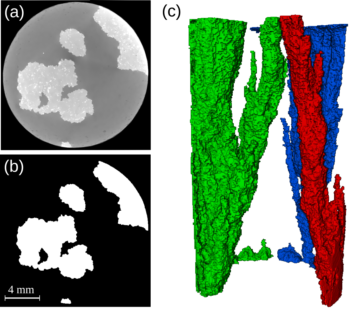
Figure 2a shows a horizontal two-dimensional slice of a tomography. The different gray values correspond to glass spheres immersed in sodium carbonate solution (dark gray), glass spheres immersed in barium chloride solution (bright gray), and barium carbonate which has precipitated onto the glass beads (white).
2.3 Image analysis
The segmentation of the 3D volume data into the two partial volumes filled by the two liquid solutions is based on the gray values of the individual voxels. Two preprocessing steps facilitate 38 this binarization: First, a bilateral filter (implemented in Avizo Fire) reduces the gray level noise while preserving the edges between areas. Second, multiplication with a radially varying factor (Matlab) removes the so called beam-hardening artifact which makes the interior of the cylinder appear less bright than its circumference. Then the 3D volume is segmented with a threshold determined using Otsu’s algorithm, effectively rendering all volume, which has been invaded by solution, white (figure 2b). In a final step, isolated binarization artifacts smaller than 0.5 are removed with a morphological transformations called opening (Avizo Fire). A three-dimensional visualization of the morphology of an injected solution is shown in figure 2c.
In order to characterize the flow morphology, we compute two measures for each tomography: the number of discrete objects formed by the injected fluid and the surface to volume ratio of these individual objects. To identify separate objects, the set of all white voxels is split into subsets of voxels which are mutually connected by their faces (Avizo Fire). In figure 2c, three such structures are identified by different colors.
Next we compute for each structure a) the total volume as the number of voxels belonging to it and b) the surface enclosed by the structure as the number of all its voxels which have at least one black voxel as neighbor. The so obtained surface to volume ratio is dimensionless as both and are measured in voxels units. The final value of a tomogram is obtained by averaging over all structures contained in it.
3 Results and discussion

3.1 The flow rate controls the flow pattern


The main result of our tomographic analysis shown in figure 3 is that the flow pattern of the solution replacing the solution changes with the flow rate . For values of larger than 0.1 ml/min, the solution advances as a cylindrical, plug-like front. For smaller we observe a transition to more ramified flows, i.e. the solution moves preferentially through some channel-like structures and in this way bypasses large areas which remain filled with stagnant solution.
A more quantitative characterization of the transition is given in Figure 4 displaying the number of discrete structures as a function of the flow rate. A plug like flow corresponds to , larger numbers indicate the formation of multiple flow fingers. The transition between these two regimes occurs around 0.1 ml/min. In figure 4b, the surface to volume ratio is shown as a function of . Higher values of indicate a higher degree of ramification of the flow pattern. In our experiments, decreases monotonically when the flow rate increases, until it reaches a plateau around 0.1 ml/min, indicating the transition to a single plug-like front.
The transition between these two flow patterns can be explained, as seen below, on the basis of a microscopic picture showing how the precipitate formed by the reaction changes the pore geometry. Before doing so, let us first confirm that hydrodynamic instabilities are not involved in the process of ramification.
3.2 Influence of the flow direction
To confirm that hydrodynamic instabilities are not at the origin of the flow patterns observed, we have analyzed the possible influence of viscous fingering (VF) or Rayleigh-Taylor (RT) instabilities that could occur due to viscous and/or density contrasts between the solutions (Table 1). The experiments are performed by injection of one of the two reactant solutions into glass beads immersed in the other solution either from the top or from the bottom of a vertical cell (Fig.5).
The VF instability arises when a less viscous fluid is displacing a more viscous one and induces a deformation of the interface into fingering patterns 39, 40. The RT instability on the other hand is a buoyancy-driven instability arising when a denser fluid lies above a less dense one in the gravity field 41. It also induces fingering patterns that have been well studied in the framework of CO2 convective dissolution 42. The most unstable case occurs when both instabilities are at play, which should be here the case when the less viscous but denser solution of BaCl2 (see Table I) displaces downwards the more viscous, less dense solution of Na2CO3. As seen on Fig.5b, this situation yields however a stable downward moving plug-flow type of displacement. This pattern is actually similar to the one obtained when the more viscous but less dense solution of Na2CO3 is displacing the barium chloride solution upwards (Fig.5c), which a potentially buoyantly unstable but viscously stable displacement. Similarly, the potentially viscously unstable but buoyantly stable case shown in Fig.5d features a plug-flow like pattern. Only the case that is stable towards both instabilities (Fig.5a) features a much more ramified flow structure. This suggests that the VF or RT are not at the origin of the filament precipitation pathways but that these are formed when the hydrodynamically stable displacement at low velocities allow for the reaction to be most effective.
3.3 Clogging as the microscopic origin of the flow pattern
The precipitation of solid barium carbonate as described by equation (2) is a fast reaction 12. Hence, the rate of formation of new (s) is controlled by the transport processes by which new educts get in contact within the reaction zone at the miscible interface between the two reactant solutions. At very low flow rates, diffusion is expected to be the dominant transport process while hydrodynamic dispersion takes over when increases. The relative contribution of these two processes can be characterized by the Péclet number 21, 43:
| (3) |
where is the average grain diameter, and m2/s is the diffusion coefficient of Barium ions in water 44. Our range of average front velocities therefore covers a range of Péclet numbers from 0.34 to 20.4 with the transition between the two morphologies occuring around =3.4. The absolute values of these Péclet numbers are subject to a systematic error because the average front velocity is only a proxy of the actual liquid velocities in the ramified flow field. Nevertheless they capture the change in the flow pattern in a qualitative way.
At low , the time scale of the global advective transport is longer than the time scale of the local diffusive transport between the two reactant solutions. Hence, at small values of or equivalently small values of and thus , the local formation of precipitate by diffusion and reaction has sufficient time to close the gaps between individual glass spheres. This leads to the formation of ”tubes” which then guide the advancing flow front. On the other hand, if the solution is injected fast enough, is larger, the advective transport takes over and the produced solid is spread out over a larger volume. In consequence, the local volume of the precipitate is not sufficient to seal off throats between glass spheres and form channels that way. The injected solution spreads then homogeneously in all directions and a plug-like displacement is observed. These trends are coherent with fingering-like instabilities due to precipitation 45 and with the fact that the effect of precipitation reactions on viscous fingering in Hele-Shaw cells has been shown to decrease when increases 46.

In order to study the viability of this hypothesis, we took additional tomographies with the aim of selectively visualizing the deposited . Figure 6a shows a sample into which a solution has first been injected at a flow rate of and has reacted with the sodium carbonate initially present. Then the system has been flooded with a volume of pure water corresponding to 15 times the pore volume of the cell at a flow rate of . This procedure removed all the remaining solution. In consequence all white areas in figure 6b,c,d represent solid .
A comparison of the X-ray tomographies before and after washing (figures 6a,b) shows that the deposit is organized in a layer like structure. The higher resolution tomographies shown in figures 6c,d show that the deposit indeed closes off the space between individual glass spheres, in that way creating effective flow boundaries. The fact that those layers are not only at the outer boundaries of the barium chloride flow finger visible in figure 6a is indicative of a stage-wise formation history of the finger: earlier boundaries ”break” with increasing pressure inside the finger. The spilled liquid then forms new boundaries at geometrically favorable locations, creating an onion-like appearance of the cross-section.

Figure 7 confirms that the transition from the ramified to the plug-like flow is also accompanied by a change of precipitation patterns. In the top row of the image, cross-sections of tomographies taken at the lowest and highest value of are shown. If we make the reasonable assumption that the barium carbonate precipitate is the most dense and therefore most white part of the image, we can binarize these cross-sections with a rather high (but unfortunately arbitrary) threshold which results in the bottom row of figure 7. Here the white area now represents the barium carbonate precipitate. At the high flow rate, the precipitate formed is distributed all over the full cross-section of the sample and therefore providing only very little guidance for the fluid flow, in agreement with the observed plug flow. At the low flow rate, the precipitate is concentrated in the finger-like flow structure.
4 Conclusions
Three-dimensional reactive flow patterns have been analyzed here experimentally in porous media consisting in beads initially immersed in a solution of sodium carbonate. Upon injecting from bottom to top a solution of barium chloride, a precipitation reaction yields solid barium carbonate. It is observed by X-ray tomography that, at low injection flow rate, the flow pattern features ramified and irregular flow paths while at higher flow rates, a plug-flow displacement is obtained. A comparison of various displacements from either top to bottom or the reverse and alternating the displacing and displaced solutions shows that hydrodynamic instabilities such as viscous fingering or the buoyancy-driven Rayleigh-Taylor instability are here ruled out in the dynamics. Instead, a higher resolution tomography analysis suggests that, at low flow rate, diffusion is more effective than advection such that the precipitation reaction is more effective to produce the solid barium carbonate that, locally, blocks the pores. This, in turn, favors the growth of specific channeled pathways. At larger flow rates, advection dominates and a plug-like flow is observed as the precipitation is less efficient in blocking the pores. These results confirm experimentally in 3D porous matrices the fact that the efficiency of mineralization and the spatio-temporal distribution of the solid phase are strongly affected by the injection flow rate. This paves the way to future work aiming at optimizing CO2 mineralization in flow conditions in real field conditions.
5 Acknowledgments
We thank Markus Benderoth for experimental support. R.M. and M.S. acknowledge financial support from BP plc. within the ExploRe program. A.D. acknowledges financial support from FRS-FNRS under the PDR CONTROL programme.
References
- Metz et al. 2005 B. Metz, O. Davidson, H. D. Coninck, M. Loos and L. Meyer, IPCC special report on carbon dioxide capture and storage, Intergovernmental Panel on Climate Change, 2005.
- Kaszuba et al. 2013 J. Kaszuba, B. Yardley and M. Andreani, Reviews in Mineralogy and Geochemistry, 2013, 77, 153–188.
- Jun et al. 2013 Y.-S. Jun, D. E. Giammar and C. J. Werth, Environm. Sc. & Techn., 2013, 47, 3–8.
- Rochelle et al. 2004 C. A. Rochelle, I. Czernichowski-Lauriol and A. E. Milodowski, The impact of chemical reactions on CO2 storage in geological formations: a brief review, Geological Society London (S.J. Baines and R.H. Worden Eds.), 2004, pp. 87–106.
- Matter et al. 2016 J. M. Matter, M. Stute, S. Ó. Snæbjörnsdottir, E. H. Oelkers, S. R. Gislason, E. S. Aradottir, B. Sigfusson, I. Gunnarsson, H. Sigurdardottir, E. Gunnlaugsson, G. Axelsson, H. A. Alfredsson, D. Wolff-Boenisch, K. Mesfin, D. F. d. l. R. Taya, J. Hall, K. Dideriksen and W. S. Broecker, Science, 2016, 352, 1312–1314.
- Tartakovsky et al. 2008 A. M. Tartakovsky, G. Redden, P. C. Lichtner, T. D. Scheibe and P. Meakin, Water Resources Research, 2008, 44, W06S04.
- Zhang et al. 2010 C. Zhang, K. Dehoff, N. Hess, M. Oostrom, T. W. Wietsma, A. J. Valocchi, B. W. Fouke and C. J. Werth, Environ. Sci. Technol. Lett., 2010, 44, 7833–7838.
- White and Ward 2012 A. R. White and T. Ward, Chaos, 2012, 22, 037114.
- Schuszter et al. 2016 G. Schuszter, F. Brau and A. De Wit, Phys. Chem. Chem. Phys., 2016, 18, 25592.
- Schuszter et al. 2016 G. Schuszter, F. Brau and A. De Wit, Environ. Sci. Technol. Lett., 2016, 3, 156.
- Brau et al. 2017 F. Brau, G. Schuszter and A. De Wit, Phys. Rev. Lett., 2017, 108, 134101.
- Schuszter and De Wit 2016 G. Schuszter and A. De Wit, J. Chem. Phys., 2016, 145, 224201.
- Krummel et al. 2013 A. T. Krummel, S. S. Datta, S. Münster and D. A. Weitz, AIChE Journal, 2013, 59, 1022–1029.
- Rose and Britton 2013 H. E. L. Rose and M. M. Britton, Microporous and Mesoporous Materials, 2013, 178, 64–68.
- Murison et al. 2015 J. Murison, R. Moosavi, M. Schulz, B. Schillinger and M. Schröter, Energy & Fuels, 2015, 6271.
- Wildenschild and Sheppard 2013 D. Wildenschild and A. P. Sheppard, Advances in Water Resources, 2013, 51, 217–246.
- Luquot and Gouze 2009 L. Luquot and P. Gouze, Chemical Geology, 2009, 265, 148–159.
- Gouze and Luquot 2011 P. Gouze and L. Luquot, Journal of Contaminant Hydrology, 2011, 120-121, 45–55.
- Luhmann et al. 2014 A. J. Luhmann, X.-Z. Kong, B. M. Tutolo, N. Garapati, B. C. Bagley, M. O. Saar and W. E. Seyfried, Chemical Geology, 2014, 380, 145–160.
- Luquot et al. 2014 L. Luquot, O. Rodriguez and P. Gouze, Transport in Porous Media, 2014, 101, 507–532.
- Vialle et al. 2014 S. Vialle, S. Contraires, B. Zinzsner, J.-B. Clavaud, K. Mahiouz, P. Zuddas and M. Zamora, Journal of Geophysical Research: Solid Earth, 2014, 119, 2828–2847.
- Garcia-Rios et al. 2015 M. Garcia-Rios, L. Luquot, J. M. Soler and J. Cama, Chemical Geology, 2015, 414, 95–108.
- Menke et al. 2016 H. P. Menke, M. G. Andrew, M. J. Blunt and B. Bijeljic, Chemical Geology, 2016, 428, 15–26.
- Qajar and Arns 2016 J. Qajar and C. H. Arns, Journal of Contaminant Hydrology, 2016, 192, 60–86.
- Al-Khulaifi et al. 2017 Y. Al-Khulaifi, Q. Lin, M. J. Blunt and B. Bijeljic, Environmental Science & Technology, 2017, 51, 4108–4116.
- Lebedev et al. 2017 M. Lebedev, Y. Zhang, M. Sarmadivaleh, A. Barifcani, E. Al-Khdheeawi and S. Iglauer, International Journal of Greenhouse Gas Control, 2017, 66, 106–119.
- Selvadurai et al. 2017 A. P. S. Selvadurai, C.-B. Couture and S. M. Rezaei Niya, Physics of Fluids, 2017, 29, 096604.
- Menke et al. 2018 H. P. Menke, C. A. Reynolds, M. G. Andrew, J. P. Pereira Nunes, B. Bijeljic and M. J. Blunt, Chemical Geology, 2018, 481, 27–37.
- Thaysen et al. 2017 E. M. Thaysen, J. M. Soler, M. Boone, V. Cnudde and J. Cama, Chemical Geology, 2017, 450, 31–43.
- Desarnaud et al. 2015 J. Desarnaud, H. Derluyn, L. Molari, S. de Miranda, V. Cnudde and N. Shahidzadeh, Journal of Applied Physics, 2015, 118, 114901.
- Suekane et al. 2017 T. Suekane, J. Ono, A. Hyodo and Y. Nagatsu, Physical Review Fluids, 2017, 2, 103902.
- Rajyaguru et al. 2019 A. Rajyaguru, E. L’Hôpital, S. Savoye, C. Wittebroodt, O. Bildstein, P. Arnoux, V. Detilleux, I. Fatnassi, P. Gouze and V. Lagneau, Chemical Geology, 2019, 503, 29–39.
- Minto et al. 2017 J. M. Minto, F. F. Hingerl, S. M. Benson and R. J. Lunn, International Journal of Greenhouse Gas Control, 2017, 64, 152–162.
- Noiriel et al. 2016 C. Noiriel, C. I. Steefel, L. Yang and D. Bernard, Advances in Water Resources, 2016, 95, 125–137.
- Godinho and Withers 2018 J. R. A. Godinho and P. J. Withers, Geochimica et Cosmochimica Acta, 2018, 222, 156–170.
- Cil et al. 2017 M. B. Cil, M. Xie, A. I. Packman and G. Buscarnera, Geophysical Research Letters, 2017, 44, 6658–6666.
- Hubbell and Seltzer 2017 J. H. Hubbell and S. M. Seltzer, X-Ray Mass Attenuation Coefficients, https://physics.nist.gov/PhysRefData/XrayMassCoef/tab3.html, 2017, National Institute of Standards and Technology (NIST).
- Weis and Schröter 2017 S. Weis and M. Schröter, Review of Scientific Instruments, 2017, 88, 051809.
- Saffman and Taylor 1958 P. G. Saffman and G. Taylor, Proceedings of the Royal Society A, 1958, 245, 312–329.
- Homsy 1987 G. Homsy, Annu. Rev. Fluid Mech., 1987, 19, 271–311.
- Sharp 1984 D. H. Sharp, Physica D, 1984, 12, 3–18.
- Thomas et al. 2018 C. Thomas, S. Dehaeck and A. De Wit, Int. J. Greenhouse Gas Control, 2018, 72, 105–116.
- Pramanik and Mishra 2015 S. Pramanik and M. Mishra, Phys. Rev. E, 2015, 91, 033006.
- Rard and Miller 1980 J. A. Rard and D. G. Miller, Journal of Chemical & Engineering Data, 1980, 25, 211–215.
- Nagatsu et al. 2014 Y. Nagatsu, Y. Ishii, Y. Tada and A. De Wit, Phys. Rev. Lett., 2014, 113, 024502.
- Nagatsu et al. 2008 Y. Nagatsu, S.-Y. Bae, Y. Kato and Y. Tada, Phys. Rev. E, 2008, 77, 067302.