F3Net: Fusion, Feedback and Focus for Salient Object Detection
Abstract
Most of existing salient object detection models have achieved great progress by aggregating multi-level features extracted from convolutional neural networks. However, because of the different receptive fields of different convolutional layers, there exists big differences between features generated by these layers. Common feature fusion strategies (addition or concatenation) ignore these differences and may cause suboptimal solutions. In this paper, we propose the F3Net to solve above problem, which mainly consists of cross feature module (CFM) and cascaded feedback decoder (CFD) trained by minimizing a new pixel position aware loss (PPA). Specifically, CFM aims to selectively aggregate multi-level features. Different from addition and concatenation, CFM adaptively selects complementary components from input features before fusion, which can effectively avoid introducing too much redundant information that may destroy the original features. Besides, CFD adopts a multi-stage feedback mechanism, where features closed to supervision will be introduced to the output of previous layers to supplement them and eliminate the differences between features. These refined features will go through multiple similar iterations before generating the final saliency maps. Furthermore, different from binary cross entropy, the proposed PPA loss doesn’t treat pixels equally, which can synthesize the local structure information of a pixel to guide the network to focus more on local details. Hard pixels from boundaries or error-prone parts will be given more attention to emphasize their importance. F3Net is able to segment salient object regions accurately and provide clear local details. Comprehensive experiments on five benchmark datasets demonstrate that F3Net outperforms state-of-the-art approaches on six evaluation metrics. Code will be released at https://github.com/weijun88/F3Net.
Introduction

Salient object detection (SOD) aims to estimate the visual significant regions of images or videos and often serves as the pre-processing step for many downstream vision tasks [\citeauthoryearWang et al.2019a]. Earlier SOD algorithms mainly rely on heuristic priors (e.g., color, texture and contrast) to generate saliency maps. However, these hand-craft features can hardly capture high-level semantic relations and context information, thus they are not robust enough to complex scenarios. Recently, convolutional neural networks (CNNs) have demonstrated its powerful feature extraction capability in visual feature representation [\citeauthoryearZhang et al.2018c, \citeauthoryearSzegedy et al.2015, \citeauthoryearHuang et al.2017, \citeauthoryearHu, Shen, and Sun2018]. Many CNNs-based models [\citeauthoryearHou et al.2019, \citeauthoryearQin et al.2019, \citeauthoryearChen et al.2018, \citeauthoryearWu, Su, and Huang2019, \citeauthoryearLi et al.2018, \citeauthoryearZhang et al.2018b, \citeauthoryearFeng, Lu, and Ding2019, \citeauthoryearWang et al.2017b, \citeauthoryearZhang et al.2017] have achieved remarkable progress and pushed the performance of SOD to a new level. These models adopt the encoder-decoder architecture, which is simple in structure and computationally efficient. The encoder usually is made up of a pre-trained classification model (e.g. ResNet [\citeauthoryearHe et al.2016] and VGG [\citeauthoryearSimonyan and Zisserman2015]), which can extract multiple features of different semantic levels and resolutions. In the decoder, extracted features are combined to generate saliency maps.
However, there still remains two big challenges in accurate SOD. First, features of different levels have different distribution characteristics. High level features have rich semantics but lack accurate location information. Low level features have rich details but full of background noises. To generate better saliency maps, multi-level features are combined. However, without delicate control of the information flow in the model, some redundant features, including noises from low level layers and coarse boundaries from high level layers will pass in and possibly result in performance degradation. Second, most of existing models use binary cross entropy that treats all pixels equally. Intuitively, different pixels deserve different weights, e.g., pixels at the boundary are more discriminative and should be attached with more importance. Various boundary losses [\citeauthoryearQin et al.2019, \citeauthoryearFeng, Lu, and Ding2019] have been proposed to enhance the boundary detection accuracy, but considering only the boundary pixels is not comprehensive enough, since there are lots of pixels near the boundaries prone to wrong predictions. These pixels are also important and should be assigned with larger weights. In consequence, it is essential to design a mechanism to reduce the impact of inconsistency between features of different levels and assign larger weights to those truly important pixels.
To address above challenges, we proposed a novel SOD framework, named F3Net, which achieves remarkable performance in producing high quality saliency maps. First, to mitigate the discrepancy between features, we design cross feature module (CFM), which fuses features of different levels by element-wise multiplication. Different from addition and concatenation, CFM takes a selective fusion strategy, where redundant information will be suppressed to avoid the contamination between features and important features will complement each other. Compared with traditional fusion methods, CFM is able to remove background noises and sharpen boundaries, as shown in Fig. 1. Second, due to downsampling, high level features may suffer from information loss and distortion, which can not be solved by CFM. Therefore, we develop the cascaded feedback decoder (CFD) to refine these features iteratively. CFD contains multiple sub-decoders, each of which contains both bottom-up and top-down processes. For bottom-up process, multi-level features are aggregated by CFM gradually. For top-down process, aggregated features are feedback into previous features to refine them. Third, we propose the pixel position aware loss (PPA) to improve the commonly used binary cross entropy loss which treats all pixels equally. In fact, pixels located at boundaries or elongated areas are more difficult and discriminating. Paying more attention to these hard pixels can further enhance model generalization. PPA loss assigns different weights to different pixels, which extends binary cross entropy. The weight of each pixel is determined by its surrounding pixels. Hard pixels will get larger weights and easy pixels will get smaller ones.
To demonstrate the performance of F3Net, we report experiment results on five popular SOD datasets and visualize some saliency maps. We conduct a series of ablation studies to evaluate the effect of each module. Quantitative indicators and visual results show that F3Net can obtained significantly better local details and improved saliency maps. Codes has been released. In short, our main contributions can be summarized as follows:
- •
We introduce the cross feature module to fuse features of different levels, which is able to extract the shared parts between features and suppress each other’s background noises and complement each other’s missing parts.
- •
We propose the cascaded feedback decoder for SOD, which can feedback features of both high resolutions and high semantics to previous ones to correct and refine them for better saliency maps generation.
- •
We design pixel position aware loss to assign different weights to different positions. It can better mine the structure information contained in the features and help the network focus more on detail regions.
- •
Experimental results demonstrate that the proposed model F3Net achieves the state-of-the-art performance on five datasets in terms of six metrics, which proves the effectiveness and superiority of the proposed method.
Related Work
Early SOD methods mainly rely on intrinsic cues, such as color contrast [\citeauthoryearCheng et al.2015], texture [\citeauthoryearYan et al.2013] and center prior [\citeauthoryearJiang and Davis2013] to extract saliency maps, which mainly focus on low-level information and ignore rich contextual semantic information. Recently, CNNs has been used to extract multi-level features from original images and aggregate the extracted features to produce saliency maps.
Among these methods, [\citeauthoryearHou et al.2019] introduced short connections in fully convolutional networks [\citeauthoryearLong, Shelhamer, and Darrell2015] to integrate features from different layers. [\citeauthoryearDeng et al.2018] and [\citeauthoryearWang et al.2017b] adopted an iterative strategy to refine the saliency maps step-by-step, using features both from deep layers and shallow layers. [\citeauthoryearLiu, Han, and Yang2018] proposed to generate attention over the context regions for each pixel, which can help suppress the interference of background noises. [\citeauthoryearChen et al.2018] and [\citeauthoryearZhang et al.2018b] used attention-guided network to select and extract supplementary features and integrate them to enhance saliency maps. [\citeauthoryearQin et al.2019] designed hybrid loss to make full use of boundary information and [\citeauthoryearFeng, Lu, and Ding2019] used a two-branch network to simultaneously predict the contours and saliency maps. [\citeauthoryearZhang et al.2018a] designed a bi-directional message passing model for better feature selection and integration. [\citeauthoryearLiu et al.2019] utilized simple pooling and feature aggregation module to build fast and high performance model. [\citeauthoryearZhao and Wu2019] introduced the channel-wise attention and spatial attention to extract valuable features and suppress background noise.
However, the discrepancy between features of different levels has not been comprehensively studied. How to design more effective fusion strategies to reduce this discrepancy has become an important problem in SOD. In addition, apart from boundaries, there are lots of hard pixels deserving more attention. Increasing their weights in loss function can further improve the discriminating ability. Based on above mentioned problems, we design F3Net to generate saliency maps accurately and efficiently.
Proposed Method
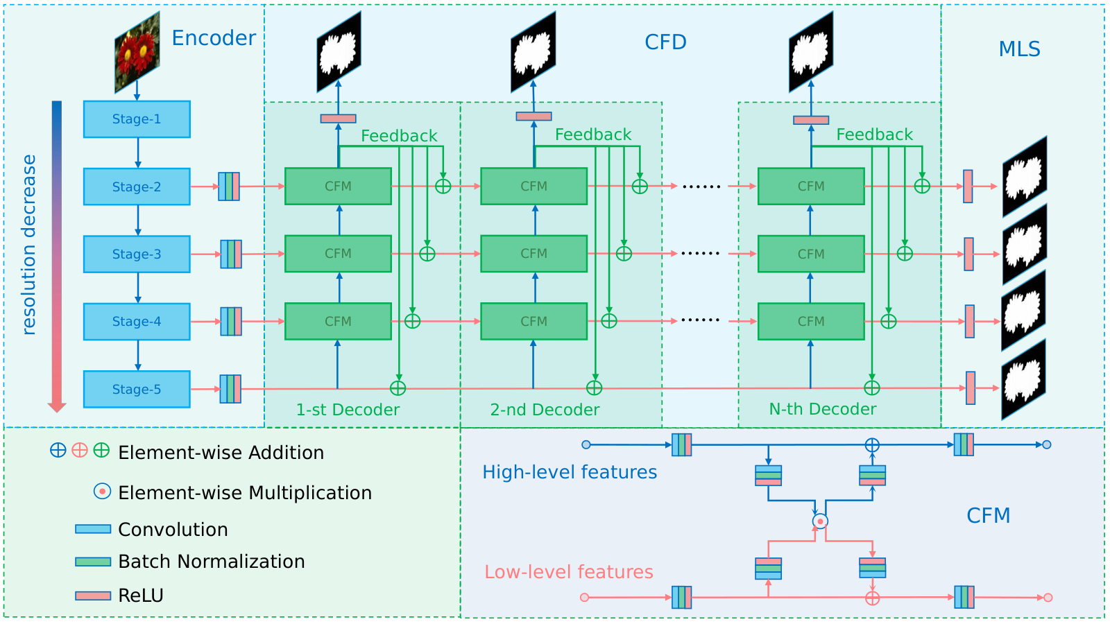
We design cross feature module to selectively integrate features, which can prevent the introduction of redundant features. To refine the saliency maps, we propose a cascaded feedback decoder to refine multi-level features by multiple iterations. To guide the network to focus more on local details, we introduce pixel position aware loss which assigns different weights to different pixels. See Fig.2 for details.
Cross Feature Module
We propose cross feature module (CFM) to refine both high level features and low level features . preserves rich details as well as background noises, due to the restriction of the receptive field. These features have clear boundaries, which are important to generate accurate saliency maps. In contrast, is coarse in boundaries, because of multiple downsamplings. Despite of losing too much detailed information, still has consistent semantics and clear background. There exists big statistical discrepancy between these two kinds of features. Some examples have been shown in Fig. 1.
CFM performs feature crossing to mitigate the discrepancy between features. It firstly extracts the common parts between and by element-wise multiplication and then combines them with original and respectively by element-wise addition. Compared with direct addition or concatenation employed in existing study, CFM avoids redundant information introduced to and , which may ”pollute” the original features and bring adverse effect to the generation of saliency maps. By multiple feature crossings, and will gradually absorb useful information from each other to complement themselves, i.e., noises of will be suppressed and boundaries of will be sharpened.
Specifically, CFM contains two branches, one for and the other for , as shown in Fig. 2. At first, one 3x3 convolutional layer is applied to and respectively to adapt them for follow-up processing. Then these features are transformed and fused by multiplication. The fused features share the properties of both and , i.e., clear boundaries and consistent semantics. Finally, the fused features will be added to the original and for refine representations. The whole process could be shown as follows.
| (1) | ||||
| (2) |
where each of is the combination of convolution, batchnorm and relu. After getting the refined features, 3x3 convolution is applied to restore the original dimensions. The whole module presents a completely symmetric structure, where embeds its details to and filters the background noises of .
Cascaded Feedback Decoder
Cascaded feedback decoder (CFD) is built upon CFM which refines the multi-level features and generate saliency maps iteratively. For SOD, traditional methods aim to directly aggregate multi-level features to produce the final saliency maps. In fact, features of different levels may have missing or redundant parts because of downsamplings and noises. Even with CFM, these parts are still difficult to identify and restore, which may hurt the final performance. Considering the output saliency map is relatively complete and approximate to ground truth, we propose to propagate the features of the last convolution layer back to features of previous layers to correct and refine them.
Fig. 2 shows the architecture of CFD which contains multiple decoders. Each decoder consists of two processes, i.e., bottom-up and top-down. For bottom-up process, features are gradually aggregated by CFM from high level to low level. The aggregated features will be supervised and produce a coarse saliency map. For top-down process, features aggregated by last process are directly downsampled and added to previous multi-level features exported by CFM to refine them. These refined features will be sent to the next decoder to go through the same processes. In fact, inside CFD, two processes of multiple decoders are linked one-by-one and form a grid net. Multi-level features are flowing and refined in this net iteratively. At last, these features will be complete enough to generate finer saliency maps.
Specifically, we build CFD on ResNet-50 [\citeauthoryearHe et al.2016], a widely used backbone in SOD tasks. For an input image with size x, ResNet-50 will extract its features at five levels, denoted as with resolutions . Because low level features bring too much computational cost but little performance improvement [\citeauthoryearWu, Su, and Huang2019], we only use features of the last four levels , which have lower resolutions and cost less computation. The whole process of CFD can be formulated as Alg. 1, where is the -th sub-decoder and means the downsampling operation.
Pixel Position Aware Loss

In SOD, binary cross entropy (BCE) is the most widely used loss function. However, BCE loss has three drawbacks. First, it calculates the loss for each pixel independently and ignores the global structure of the image. Second, in pictures where the background is dominant, loss of foreground pixels will be diluted. Third, it treats all pixels equally. In fact, pixels located on cluttered or elongated areas (e.g., pole and horn) are prone to wrong predictions and deserve more attention and pixels located areas, like sky and grass, deserve less attention. So we propose a weighted binary cross entropy (wBCE) loss as shown in Eq. 3
| (3) |
where is the indicator function and is a hyper-parameter. The notation indicates two kinds of the labels. and are prediction and ground truth of the pixel at location in an image. represents all the parameters of the model and denotes the predicted probability.
In , each pixel will be assigned with a weight . Hard pixel corresponds to larger and simple pixel will be assigned a smaller one. could be regarded as the indicator of pixel importance, which is calculated according to the difference between the center pixel and its surroundings, Eq. 4.
| (4) |
where represents the area that surrounds the pixel . For all pixels, . If is large, pixel at is very different from its surroundings. So it is an important pixel (e.g., edge or hole) and deserves more attention. On the contrary, if is small, we think it is a plain pixel and deserve less attention. Fig. 3 has shown some examples.
Compared with BCE, pays more attention hard pixels. In addition, local structure information has been encoded into , which may help the model focus on a larger receptive field rather than on a single pixel. To further make the network focus on global structure, we introduce weighted IoU (wIoU) loss, as shown in Eq. 5.
| (5) |
IoU loss has been widely used in image segmentation [\citeauthoryearRahman and Wang2016]. It aims to optimize the global structure instead of focusing on single pixel and it is not affected by the unbalanced distribution. Recently, it has been introduced into SOD [\citeauthoryearQin et al.2019] to make up for the deficiency of BCE. But it still treats all pixels equally and ignores the difference between pixels. Different from IoU loss, our wIoU loss assigns more weights to hard pixels to emphasize their importance.
Based on above discussion, the pixel position aware loss is shown in Eq. 6. It synthesizes local structure information to generate different weights for all pixels and introduce both pixel restriction () and global restriction (), which can better guide the network learning and produce clear details.
| (6) |
Each sub-decoder in CFD corresponds to one . Besides, multi-level supervision (MLS) is added as an auxiliary loss to facilitate sufficient training, as shown in Fig. 2. Given sub-decoders in CFD and levels in total, the whole loss is defined in Eq. 7
| (7) |
The first item corresponds to the mean of all sub-decoders’ loss and the second corresponds to the weighted sum of auxiliary loss where high level loss has smaller weight because of its larger error.
Experiments
| Algorithm | ECSSD | PASCAL-S | DUTS-TE | HKU-IS | DUT-OMRON | |||||||||||||||
|---|---|---|---|---|---|---|---|---|---|---|---|---|---|---|---|---|---|---|---|---|
| 1,000 images | 850 images | 5,019 images | 4,447 images | 5,168 images | ||||||||||||||||
| MAE | MAE | MAE | MAE | MAE | ||||||||||||||||
| C2SNet(ECCV2018) | .059 | .853 | .882 | .906 | .086 | .761 | .822 | .835 | .066 | .710 | .817 | .841 | .051 | .839 | .873 | .919 | .079 | .664 | .780 | .817 |
| RAS(ECCV2018) | .055 | .890 | .894 | .916 | .102 | .782 | .792 | .832 | .060 | .750 | .838 | .861 | .045 | .874 | .888 | .931 | .063 | .711 | .812 | .843 |
| R3Net(IJCAI2018) | .051 | .883 | .910 | .914 | .101 | .775 | .809 | .824 | .067 | .716 | .837 | .827 | .047 | .853 | .894 | .921 | .073 | .690 | .819 | .814 |
| PiCA-R(CVPR2018) | .046 | .886 | .917 | .913 | .075 | .798 | .849 | .833 | .051 | .759 | .869 | .862 | .043 | .870 | .904 | .936 | .065 | .717 | .832 | .841 |
| BMPM(CVPR2018) | .044 | .894 | .911 | .914 | .073 | .803 | .840 | .838 | .049 | .762 | .861 | .859 | .039 | .875 | .906 | .937 | .063 | .698 | .809 | .839 |
| DGRL(CVPR2018) | .043 | .903 | .906 | .917 | .074 | .807 | .834 | .836 | .051 | .764 | .846 | .863 | .037 | .881 | .896 | .941 | .063 | .709 | .810 | .843 |
| PAGE(CVPR2019) | .042 | .906 | .912 | .920 | .077 | .810 | .835 | .841 | .052 | .777 | .854 | .869 | .037 | .882 | .903 | .940 | .062 | .736 | .824 | .853 |
| AFNet(CVPR2019) | .042 | .908 | .913 | .918 | .070 | .821 | .844 | .846 | .046 | .792 | .867 | .879 | .036 | .888 | .905 | .942 | .057 | .738 | .826 | .853 |
| TDBU(CVPR2019) | .041 | .880 | .918 | .922 | .071 | .779 | .844 | .852 | .048 | .767 | .865 | .879 | .038 | .878 | .907 | .942 | .061 | .739 | .837 | .854 |
| PoolNet(CVPR2019) | .039 | .915 | .921 | .924 | .074 | .822 | .845 | .850 | .040 | .809 | .883 | .889 | .032 | .899 | .916 | .949 | .055 | .747 | .835 | .863 |
| BASNet(CVPR2019) | .037 | .880 | .916 | .921 | .076 | .775 | .832 | .847 | .048 | .791 | .866 | .884 | .032 | .895 | .909 | .946 | .056 | .756 | .836 | .869 |
| CPD-R(CVPR2019) | .037 | .917 | .918 | .925 | .072 | .824 | .842 | .849 | .043 | .805 | .869 | .886 | .034 | .891 | .905 | .944 | .056 | .747 | .825 | .866 |
| F3Net(ours) | .033 | .925 | .924 | .927 | .062 | .840 | .855 | .859 | .035 | .840 | .888 | .902 | .028 | .910 | .917 | .953 | .053 | .766 | .838 | .870 |

| BCE | IoU | PPA | MLS | CFM | CFD | DUTS-TE | |||
|---|---|---|---|---|---|---|---|---|---|
| MAE | |||||||||
| ✓ | .051 | .779 | .861 | .871 | |||||
| ✓ | .047 | .783 | .864 | .874 | |||||
| ✓ | ✓ | .045 | .789 | .867 | .875 | ||||
| ✓ | .043 | .808 | .872 | .880 | |||||
| ✓ | ✓ | .040 | .812 | .875 | .882 | ||||
| ✓ | ✓ | ✓ | .036 | .831 | .884 | .893 | |||
| ✓ | ✓ | ✓ | ✓ | .035 | .840 | .888 | .902 | ||
| DUT-OMRON | DUTS-TE | |||||||
|---|---|---|---|---|---|---|---|---|
| MAE | MAE | |||||||
| =3 | .058 | .755 | .835 | .857 | .038 | .835 | .888 | .898 |
| =4 | .057 | .758 | .837 | .859 | .037 | .837 | .888 | .900 |
| =5 | .053 | .766 | .838 | .870 | .035 | .840 | .888 | .902 |
| =6 | .060 | .752 | .833 | .855 | .038 | .834 | .887 | .897 |
| DUT-OMRON | DUTS-TE | |||||||
|---|---|---|---|---|---|---|---|---|
| MAE | MAE | |||||||
| =1 | .055 | .760 | .834 | .866 | .037 | .838 | .886 | .897 |
| =2 | .053 | .766 | .838 | .870 | .035 | .840 | .888 | .902 |
| =3 | .057 | .762 | .837 | .867 | .036 | .837 | .887 | .900 |
| =4 | .059 | .758 | .833 | .863 | .038 | .835 | .885 | .896 |
Datasets and Evaluation Metrics
The performance of F3Net is evaluated on five popular datasets, including ECSSD [\citeauthoryearYan et al.2013] with 1000 images, PASCAL-S [\citeauthoryearLi et al.2014] with 850 images, DUT-OMRON [\citeauthoryearYang et al.2013] with 5168 images, HKU-IS [\citeauthoryearLi and Yu2015] with 4,447 images and DUTS [\citeauthoryearWang et al.2017a] with 15,572 images. All datasets are human-labeled with pixel-wise ground-truth for quantitative evaluations. DUTS is currently the largest SOD dataset, which are divided into 10,553 training images (DUTS-TR) and 5,019 testing images (DUTS-TE). We follow [\citeauthoryearWu, Su, and Huang2019, \citeauthoryearQin et al.2019] to use DUTS-TR as the training dataset and others as testing datasets.
In addition, six metrics are used to evaluate the performance of F3Net and existing state-of-the-art methods. The first metric is the mean absolute error (MAE), as shown in Eq. 8, which is widely adopted in [\citeauthoryearHou et al.2019, \citeauthoryearLiu, Han, and Yang2018]. Mean F-measure (), structural similarity measure () [\citeauthoryearFan et al.2017] and E-measure () [\citeauthoryearFan et al.2018] are also widely used to evaluate salient maps. In addition, precision-recall (PR) and F-measure curves are drawn to show the whole performance.
| (8) |
where is the predicted map and is the ground truth.
Implementation Details
DUTS-TR is used to train F3Net and other above mentioned datasets are used to evaluate F3Net. For data augmentation, we use horizontal flip, random crop and multi-scale input images. ResNet-50 [\citeauthoryearHe et al.2016], pre-trained on ImageNet, is used as the backbone network. Maximum learning rate is set to 0.005 for ResNet-50 backbone and 0.05 for other parts. Warm-up and linear decay strategies are used to adjust the learning rate. The whole network is trained end-to-end, using stochastic gradient descent (SGD). Momentum and weight decay are set to 0.9 and 0.0005, respectively. Batchsize is set to 32 and maximum epoch is set to 32. We use Pytorch 1.3 to implement our model. An RTX 2080Ti GPU is used for acceleration. During testing, we resized each image to 352 x 352 and then feed it to F3Net to predict saliency maps without any post-processing. Codes has been released at https://github.com/weijun88/F3Net.
Ablation Studies
Before analyzing the influence of each module, there are two hyper parameters (i.e., and ) to be determined. is used in PPA loss to adjust the proportion of hard pixels. Tab.3 lists the scores of , , and when is given different values. As can be seen, when equals 5, these indicators reach highest scores. In addition, represents the number of sub-decoders in CFD. We increase gradually from 1 to 4 and measure the corresponding scores of above metrics, as shown in Tab. 4. When =2, the model achieves the best performance. Both of these experiments are conducted on DUT-OMRON and DUTS.
To investigate the importance of different modules in F3Net, we conduct a series of controlled experiments on DUTS, as shown in Tab.2. First, we test the effect of different loss functions, inlcuding BCE, IoU and PPA. Among them, PPA loss achieves the best performance on three evaluation metrics. Furthermore, we keep adding the multi-level supervision, cross feature module and cascaded feedback decoder to evaluate their performance. As we can see, all these modules boost the model performance. When these modules are combined, we can get the best SOD results. It demonstrates that all components are necessary for the proposed framework.
Comparison with State-of-the-arts
Quantitative Comparison. To demonstrate the effectiveness of the proposed F3Net, we compare it against 12 state-of-the-art SOD algorithms, including AFNet [\citeauthoryearFeng, Lu, and Ding2019], BASNet [\citeauthoryearQin et al.2019], CPD-R [\citeauthoryearWu, Su, and Huang2019], BMPM [\citeauthoryearZhang et al.2018a], R3Net [\citeauthoryearDeng et al.2018], PiCA-R [\citeauthoryearLiu, Han, and Yang2018], DGRL [\citeauthoryearWang et al.2018], TDBU [\citeauthoryearWang et al.2019b], PoolNet [\citeauthoryearLiu et al.2019], PAGE [\citeauthoryearWang et al.2019c], RAS [\citeauthoryearChen et al.2018] and C2SNet [\citeauthoryearLi et al.2018]. For fair comparison, we use all saliency maps provided by the authors and evaluate them with the same code. As shown in Tab.1, our approach achieves the best scores across five datasets with respect to four metrics, compared with other counterparts. It demonstrates the superior performance of the proposed F3Net. In addition, Fig. 4 shows the precision-recall curves of above mentioned algorithms on five datasets, which can evaluate the holistic performance of models. From these curves, we can observe that F3Net consistently outperforms all other models under different thresholds, which means that our method have a good capability to detect salient regions as well as generate accurate saliency maps.
Visual Comparison. In order to evaluate the proposed F3Net, we visualize some saliency maps produced by our model and other approaches in Fig. 5. We observe that the proposed method not only highlights the salient object regions clearly, but also well suppresses the background noises. It excels in dealing with various challenging scenarios, including cluttered backgrounds (row 2 and 6), small objects (row3), inverted reflection in water (row1) and occlusion (row 2). Compared with other counterparts, the saliency maps produced by our method are clearer and more accurate. Most importantly, our method achieves these results without any post-processing.
Conclusion
In this paper, we propose a novel SOD framework named F3Net. First, considering the difference between features of different levels, we propose CFM to selectively integrate features, which prevents the improper influence of redundant features. To further get finer details, we introduce CFD to refine multi-level features iteratively with feedback mechanisms. Besides, we design PPA loss to pay more attention to hard pixels and guide the network focus more on error-prone parts. The whole framework demonstrates remarkable feature extraction capability, which makes it robust and effective in various challenging scenarios. Experimental results on five datasets demonstrate that F3Net outperforms state-of-the-art methods under six evaluation metrics.
Acknowledgement
This work was supported in part by National Natural Science Foundation of China: 61672497, 61620106009, 61931008, U1636214 and 61836002, and in part by Key Research Program of Frontier Sciences, CAS: QYZDJ-SSW-SYS013.
References
- [\citeauthoryearChen et al.2018] Chen, S.; Tan, X.; Wang, B.; and Hu, X. 2018. Reverse attention for salient object detection. In ECCV (9), volume 11213 of Lecture Notes in Computer Science, 236–252. Springer.
- [\citeauthoryearCheng et al.2015] Cheng, M.; Mitra, N. J.; Huang, X.; Torr, P. H. S.; and Hu, S. 2015. Global contrast based salient region detection. TPAMI 37(3):569–582.
- [\citeauthoryearDeng et al.2018] Deng, Z.; Hu, X.; Zhu, L.; Xu, X.; Qin, J.; Han, G.; and Heng, P. 2018. R3net: Recurrent residual refinement network for saliency detection. In IJCAI, 684–690. ijcai.org.
- [\citeauthoryearFan et al.2017] Fan, D.; Cheng, M.; Liu, Y.; Li, T.; and Borji, A. 2017. Structure-measure: A new way to evaluate foreground maps. In ICCV, 4558–4567. IEEE Computer Society.
- [\citeauthoryearFan et al.2018] Fan, D.; Gong, C.; Cao, Y.; Ren, B.; Cheng, M.; and Borji, A. 2018. Enhanced-alignment measure for binary foreground map evaluation. In IJCAI, 698–704. ijcai.org.
- [\citeauthoryearFeng, Lu, and Ding2019] Feng, M.; Lu, H.; and Ding, E. 2019. Attentive feedback network for boundary-aware salient object detection. In CVPR.
- [\citeauthoryearHe et al.2016] He, K.; Zhang, X.; Ren, S.; and Sun, J. 2016. Deep residual learning for image recognition. In CVPR, 770–778. IEEE Computer Society.
- [\citeauthoryearHou et al.2019] Hou, Q.; Cheng, M.; Hu, X.; Borji, A.; Tu, Z.; and Torr, P. H. S. 2019. Deeply supervised salient object detection with short connections. TPAMI 41(4):815–828.
- [\citeauthoryearHu, Shen, and Sun2018] Hu, J.; Shen, L.; and Sun, G. 2018. Squeeze-and-excitation networks. In CVPR, 7132–7141. IEEE Computer Society.
- [\citeauthoryearHuang et al.2017] Huang, G.; Liu, Z.; van der Maaten, L.; and Weinberger, K. Q. 2017. Densely connected convolutional networks. In CVPR, 2261–2269. IEEE Computer Society.
- [\citeauthoryearJiang and Davis2013] Jiang, Z., and Davis, L. S. 2013. Submodular salient region detection. In CVPR, 2043–2050. IEEE Computer Society.
- [\citeauthoryearLi and Yu2015] Li, G., and Yu, Y. 2015. Visual saliency based on multiscale deep features. In CVPR, 5455–5463. IEEE Computer Society.
- [\citeauthoryearLi et al.2014] Li, Y.; Hou, X.; Koch, C.; Rehg, J. M.; and Yuille, A. L. 2014. The secrets of salient object segmentation. In CVPR, 280–287. IEEE Computer Society.
- [\citeauthoryearLi et al.2018] Li, X.; Yang, F.; Cheng, H.; Liu, W.; and Shen, D. 2018. Contour knowledge transfer for salient object detection. In ECCV (15), volume 11219 of Lecture Notes in Computer Science, 370–385. Springer.
- [\citeauthoryearLiu et al.2019] Liu, J.; Hou, Q.; Cheng, M.; Feng, J.; and Jiang, J. 2019. A simple pooling-based design for real-time salient object detection. In CVPR, 3917–3926.
- [\citeauthoryearLiu, Han, and Yang2018] Liu, N.; Han, J.; and Yang, M. 2018. Picanet: Learning pixel-wise contextual attention for saliency detection. In CVPR, 3089–3098. IEEE Computer Society.
- [\citeauthoryearLong, Shelhamer, and Darrell2015] Long, J.; Shelhamer, E.; and Darrell, T. 2015. Fully convolutional networks for semantic segmentation. In CVPR, 3431–3440. IEEE Computer Society.
- [\citeauthoryearQin et al.2019] Qin, X.; Zhang, Z.; Huang, C.; Gao, C.; Dehghan, M.; and Jagersand, M. 2019. Basnet: Boundary-aware salient object detection. In CVPR.
- [\citeauthoryearRahman and Wang2016] Rahman, M. A., and Wang, Y. 2016. Optimizing intersection-over-union in deep neural networks for image segmentation. In ISVC (1), volume 10072 of Lecture Notes in Computer Science, 234–244. Springer.
- [\citeauthoryearSimonyan and Zisserman2015] Simonyan, K., and Zisserman, A. 2015. Very deep convolutional networks for large-scale image recognition. In ICLR.
- [\citeauthoryearSzegedy et al.2015] Szegedy, C.; Liu, W.; Jia, Y.; Sermanet, P.; Reed, S. E.; Anguelov, D.; Erhan, D.; Vanhoucke, V.; and Rabinovich, A. 2015. Going deeper with convolutions. In CVPR, 1–9. IEEE Computer Society.
- [\citeauthoryearWang et al.2017a] Wang, L.; Lu, H.; Wang, Y.; Feng, M.; Wang, D.; Yin, B.; and Ruan, X. 2017a. Learning to detect salient objects with image-level supervision. In CVPR, 3796–3805. IEEE Computer Society.
- [\citeauthoryearWang et al.2017b] Wang, T.; Borji, A.; Zhang, L.; Zhang, P.; and Lu, H. 2017b. A stagewise refinement model for detecting salient objects in images. In ICCV, 4039–4048. IEEE Computer Society.
- [\citeauthoryearWang et al.2018] Wang, T.; Zhang, L.; Wang, S.; Lu, H.; Yang, G.; Ruan, X.; and Borji, A. 2018. Detect globally, refine locally: A novel approach to saliency detection. In CVPR, 3127–3135. IEEE Computer Society.
- [\citeauthoryearWang et al.2019a] Wang, W.; Lai, Q.; Fu, H.; Shen, J.; and Ling, H. 2019a. Salient object detection in the deep learning era: An in-depth survey. arXiv preprint arXiv:1904.09146.
- [\citeauthoryearWang et al.2019b] Wang, W.; Shen, J.; Cheng, M.; and Shao, L. 2019b. An iterative and cooperative top-down and bottom-up inference network for salient object detection. In CVPR, 5968–5977.
- [\citeauthoryearWang et al.2019c] Wang, W.; Zhao, S.; Shen, J.; Hoi, S. C. H.; and Borji, A. 2019c. Salient object detection with pyramid attention and salient edges. In CVPR, 1448–1457.
- [\citeauthoryearWu, Su, and Huang2019] Wu, Z.; Su, L.; and Huang, Q. 2019. Cascaded partial decoder for fast and accurate salient object detection. In CVPR.
- [\citeauthoryearYan et al.2013] Yan, Q.; Xu, L.; Shi, J.; and Jia, J. 2013. Hierarchical saliency detection. In CVPR, 1155–1162. IEEE Computer Society.
- [\citeauthoryearYang et al.2013] Yang, C.; Zhang, L.; Lu, H.; Ruan, X.; and Yang, M. 2013. Saliency detection via graph-based manifold ranking. In CVPR, 3166–3173. IEEE Computer Society.
- [\citeauthoryearZhang et al.2017] Zhang, P.; Wang, D.; Lu, H.; Wang, H.; and Ruan, X. 2017. Amulet: Aggregating multi-level convolutional features for salient object detection. In ICCV, 202–211. IEEE Computer Society.
- [\citeauthoryearZhang et al.2018a] Zhang, L.; Dai, J.; Lu, H.; He, Y.; and Wang, G. 2018a. A bi-directional message passing model for salient object detection. In CVPR, 1741–1750. IEEE Computer Society.
- [\citeauthoryearZhang et al.2018b] Zhang, X.; Wang, T.; Qi, J.; Lu, H.; and Wang, G. 2018b. Progressive attention guided recurrent network for salient object detection. In CVPR, 714–722. IEEE Computer Society.
- [\citeauthoryearZhang et al.2018c] Zhang, Z.; Zhang, X.; Peng, C.; Xue, X.; and Sun, J. 2018c. Exfuse: Enhancing feature fusion for semantic segmentation. In ECCV (10), volume 11214 of Lecture Notes in Computer Science, 273–288. Springer.
- [\citeauthoryearZhao and Wu2019] Zhao, T., and Wu, X. 2019. Pyramid feature attention network for saliency detection. In CVPR.