Interarea Oscillations & Chimera in Power Systems

The basic elements of a power grid consists of active generators and passive machines/loads. The generator converts some source of energy into electrical power which is produced by the prime mover of the generator with the frequency close to the standard or natural frequency $\Omega$ of an electrical system. All generators in a power grid can be looked upon as set of synchronous machines rotating at synchronous frequency $\Omega$, with the stator windings of the generator delivering electrical power to the grid. Any power generator in a power system is described by a power balance equation of the form,

$$P_{accumulated}+P_{dissipated}=P_{source}-P_{transmitted},$$

(2)

where $P_{source}$ is the rate at which the energy is fed into the generator at frequency $\Omega$ (i.e., $2\pi\Omega=50$Hz). Hence, the phase angle $\theta_{i}$ at the output of the $i$-th generator in stationary frame is then given by,

$$\theta_{i}=\Omega t+\delta_{i}.$$

(3)

$P_{accumulated}$ is the rate at which kinetic energy is accumulated by the generator:

$$P_{accumulated}=\frac{1}{2}J_{i}\frac{d}{dt}(\dot{\theta}_{i})^{2},$$

(4)

where $J_{i}$ is the moment of inertia of the $i$-th generator in kgm². For the sake of simplicity, we assume identical machines (i.e., $J_{i}=J$). $P_{transmitted}$ is the power transmitted from generator $i$ to $j$ with phase difference, $\Delta\theta_{ij}=\theta_{j}-\theta_{i}\neq 0$.

$$P_{transmitted}=-P_{max}sin(\Delta\theta_{ij}).$$

(5)

$P_{max}$ being maximum electrical power input in watts. The dissipated power ($P_{dissipated}$) with $K_{D}$ the dissipation constant of the prime mover in Ws²/rad², can be expressed as:

$$P_{dissipated}=K_{D}(\dot{\theta}_{i})^{2}.$$

(6)

Since, all the generators share common frequencies $\Omega$, $\Delta\theta_{ij}=\Delta\delta_{ij}=\Phi_{ij}$. Substituting (4), (5) and (6) in (2), following can be computed,

$$P_{source}=J\ddot{\theta}_{i}\dot{\theta}_{i}+K_{D}(\dot{\theta}_{i})^{2}-P_{max}sin(\Phi_{ij}).$$

(7)

Differentiating (3) with respect to time and further double differentiating it; thereby assuming perturbations around the synchronous frequency being very small, $i.e.,\dot{\delta}_{i}\ll\Omega$, (7) can be approximated as,

$$P_{source}\cong J\Omega\ddot{\delta}_{i}+[J\ddot{\delta}_{i}+2K_{D}\Omega]\dot{\delta}_{i}+K_{D}\Omega^{2}-P_{max}sin(\Phi_{ij}).$$

(8)

Under practically relevant assumptions, the coefficient of first derivative is constant and neglecting acceleration terms, as well as knowing that the rate at which the energy is stored in kinetic term is much lower as compared to rate at which energy is dissipated in friction, (8) is reduced to,

$$J\Omega\ddot{\delta}_{i}=P_{source}-K_{D}\Omega^{2}-2K_{D}\Omega\dot{\delta}_{i}+P_{max}sin(\Phi_{ij}).$$

(9)

Now, using the fact that, $P_{max}=E_{i}E_{j}\left|Y_{ij}\right|$; $E_{i}$ being internal voltage of $i$-th generator, $Y_{ij}$ the Kron reduced admittance matrix denoting maximum power transferred between generators [13] and choosing $P_{m,i}=P_{source}-K_{D}\Omega^{2}$, where $P_{m,i}$ is the mechanical power input,

$$J\Omega\ddot{\delta}_{i}=P_{m,i}-E^{2}_{i}\Re(Y_{ii})-2K_{D}\Omega\dot{\delta}_{i}+\sum_{j\neq i,j=1}^{n}E_{i}E_{j}\left|Y_{ij}\right|sin(\Phi_{ij}).$$

(10)

Dividing both sides by $J\Omega$,

$$\ddot{\delta}_{i}=\left[\frac{P_{m,i}}{J\Omega}-\frac{E^{2}_{i}\Re(Y_{ii})}{J\Omega}\right]-\frac{2K_{D}}{J}\dot{\delta}_{i}+\sum_{j\neq i,j=1}^{n}\frac{E_{i}E_{j}\left|Y_{ij}\right|}{J\Omega}sin(\Phi_{ij}).$$

(11)

(11) can be rewritten as follows,

$$\ddot{\delta}_{i}=\omega_{i}-\alpha\dot{\delta}_{i}+\sum_{j\neq i,j=1}^{n}k_{ij}sin(\delta_{j}-\delta_{i}),$$

(12)

where $\alpha=\frac{2K_{D}}{J}$ is the dissipation constant, coupling constant $[k_{ij}]=\frac{E_{i}E_{j}\left|Y_{ij}\right|}{J\Omega}$ and natural frequency $\omega_{i}=\left[\frac{P_{m,i}}{J\Omega}-\frac{E^{2}_{i}\Re(Y_{ii})}{J\Omega}\right]$. From a graph theoretic viewpoint $[k_{ij}]$ can be seen as a weighted laplacian matrix with $k_{ij}=0$ when generators are not connected to each other and $k_{ij}\geq\frac{(\omega_{max}-\omega_{min})n}{(2(n-1))}$ otherwise (i.e., assumed to be greater than critical coupling, to ensure steady state synchronization [13]). It can be observed that, (12) has the same form as a second order Kuramoto oscillator model [13].

Further, we extend (12) to spring coupled oscillators. In Kuramoto oscillators or spring coupled pendulums for that sake; the coupling term introduces restoring forces on the oscillators. Considering the special case, when there is no energy transfer between oscillators, either of in-phase or anti-phase steady state oscillations may exist (as observed in a spring coupled pendulum - Figure 1). For the in-phase oscillations, the restoring forces are zero implying absence of the coupling term, which is not a tangible explanation for a coupled system in practice because there would always be some sort of restoring forces present in a coupled system. On the other hand, in the case of anti-phase oscillations the spring keeps contributing restoring forces whilst the energy transfer is zero [16]. This also explains Huygens observations [17] and is a valid template for modeling interarea oscillations in power systems.

Any oscillator of the form given in (12), assuming damping/dissipation constant to be zero, with identical natural frequencies ($\omega_{i}=\omega$) and $H(\Phi_{ij})=\sum_{j\neq i,j=1}^{n}k_{ij}sin(\Phi_{ij})$ and $\Phi_{ij}=(\delta_{j}-\delta_{i})=(\theta_{j}-\theta_{i})$, can be written as,

$$\ddot{\delta}_{i}=\omega+H(\Phi_{ij}),$$

(13)

and thereby, following can be deduced,

$$\ddot{\Phi}_{ij}=H(-\Phi_{ij})-H(\Phi_{ij})=-2H(\Phi_{ij}).$$

(14)

The above (14) has fixed points $\Phi_{ij}=\beta(2\pi)$ or $\Phi_{ij}=(2\beta-1)\pi;\forall\beta\in\mathbb{Z}$ which are respectively the in-phase and anti-phase modes of the oscillator. Linearizing (14) about its fixed points,

$$\begin{split}\ddot{\Phi}_{ij}&\approx\left[-2\frac{\partial H(\Phi_{ij})}{\partial\Phi_{ij}}\Bigr|_{\begin{subarray}{c}H(\Phi_{ij})=0\end{subarray}}\right]\Phi_{ij},\\ &\approx\left[-2k_{ij}cos(\Phi_{ij})\Bigr|_{\begin{subarray}{c}H(\Phi_{ij})=0\end{subarray}}\right]\Phi_{ij}.\end{split}$$

(15)

Thus, from (15) it can be deduced that in-phase solution $\Phi_{ij}=0$ is synchronizing and stable, whereas anti-phase solution $\Phi_{ij}=\pi$ is desynchronizing and unstable. These results are similar to small-signal stability analysis performed by linearizing the nonlinear power system dynamics [2]. Hence, next we integrate these equilibrium/critical modes directly in the nonlinear dynamics of Kuramoto model (12). The in-phase or ‘conformist’ model of Kuramoto oscillators can be given as follows,

$$\ddot{\delta}_{i}=\omega_{i}-\alpha_{i}\dot{\delta}_{i}\ \hbox{\pagecolor{yellow}$\displaystyle{{+}}$}\sum_{j\neq i,j=1}^{n}k_{ij}sin(\delta_{j}-\delta_{i}),$$

(16)

whereas, an anti-phase or ‘contrarian’ Kuramoto model can be obtained by replacing $H(\Phi_{ij})$ with $-H(\Phi_{ij})$ in (13) to give,

$$\ddot{\delta}_{i}=\omega_{i}-\alpha_{i}\dot{\delta}_{i}\ \hbox{\pagecolor{green}$\displaystyle{{-}}$}\sum_{j\neq i,j=1}^{n}k_{ij}sin(\delta_{j}-\delta_{i}).$$

(17)

Linearisation of the ‘contrarian’ model (17) on the lines of (15) yields $\ddot{\Phi}_{ij}\leq 0$ for anti-phase modes and otherwise for in-phase modes. Thus, in the ‘contrarian’ model the anti-phase mode is stable and in-phase mode is unstable. All oscillations in physical systems in general and power systems in particular are weighted sum of in-phase and anti-phase modes. Hence, to study the oscillations in power systems, we propose the CC-Kuramoto model of coupled oscillators given as,

$$\begin{split}\ddot{\delta}^{a_{1}}_{i}=\omega_{i}-\alpha_{i}\dot{\delta}^{a_{1}}_{i}&\ \hbox{\pagecolor{yellow}$\displaystyle{{+}}$}\sum_{j\neq i,j=1}^{p}k_{ij}sin(\delta_{j}^{a_{1}}-\delta^{a_{1}}_{i})\\ &\ \hbox{\pagecolor{green}$\displaystyle{{-}}$}\sum_{j=p+1}^{n}k_{ij}sin(\delta^{a_{2}}_{j}-\delta^{a_{1}}_{i}),\\ \ddot{\delta}^{a_{2}}_{i}=\omega_{i}-\alpha_{i}\dot{\delta}^{a_{2}}_{i}&\ \hbox{\pagecolor{yellow}$\displaystyle{{+}}$}\sum_{j\neq i,j=p+1}^{n}k_{ij}sin(\delta_{j}^{a_{2}}-\delta^{a_{2}}_{i})\\ &\ \hbox{\pagecolor{green}$\displaystyle{{-}}$}\sum_{j=1}^{p}k_{ij}sin(\delta^{a_{1}}_{j}-\delta^{a_{2}}_{i}),\\ \end{split}$$

(18)

where without loss of generality we assume $\delta_{i}^{a_{c}}\in\big[\delta_{1}^{a_{1}},\delta_{2}^{a_{1}},\delta_{3}^{a_{2}},\delta_{4}^{a_{2}}\big]$, $p$ set of generators in area 1 ($a_{1}$) and $(n-p)$ generators in area 2 ($a_{2}$).

Further, a CC-Kuramoto model settles into one of the three type of states, depending upon the system parameters and initial conditions: Incoherent state - a state of complete desynchronization, $\pi$-state - when two groups of coherent oscillators are separated by phase difference of $\pi$ radians and the Travelling wave state - where the two coherent groups are apart by a phase difference less than $\pi$ radians. Not only do the above states exhibit rich dynamical behavior but other interesting outcomes arise in the process of transition between these states. The direct relation between CC-Kuramoto and the power system network facilitates the study of complex dynamics arising in power networks.

In order to validate the proposed model, we use a classical two-area four-machine power system commonly referred to for interarea oscillation analysis [2]. The system is symmetric; consisting of two identical areas connected through a relatively weak tie ($J_{i}=J=0.4$kgm², $\alpha_{i}=\alpha=0.125$). Each area includes two synchronous generators with equal power output. The single line diagram of the system considered is as shown in Figure 2,

All loads are represented as constant impedances. The tie-line impedance was varied by changing the number of tie circuits in service. Power transfer between two areas is emulated, either by an uneven distribution of generation between the areas, or by an uneven split of the total system loads. The combinations for tie-line power flow are given in Table 1.

The number of tie-line in service is two and the transfer level along the tie-line of the two areas varies from 0 to 400 MW due to the variation of load levels in the two areas. Case 1 relates to no power transfer between two areas. On the other hand, the event of power transfer between areas has been designated as Case 2.

$\displaystyle K_{Case1}=\begin{bmatrix}0&1.9689&0.1766&0.1782\\ 1.9689&0&0.1782&0.1801\\ 0.1766&0.1782&0&1.9363\\ 0.1782&0.1801&1.9363&0\end{bmatrix}$

(19)

$\displaystyle K_{Case2}=\begin{bmatrix}0&2.5960&0.2130&0.2151\\ 2.5960&0&0.2151&0.2171\\ 0.2130&0.2151&0&1.7214\\ 0.2151&0.2171&1.7214&0\end{bmatrix}$

(20)

The coupling matrix $[k_{ij}]$ is represented as (19) for Case 1 and (20) for Case 2. Elements of coupling matrix $[k_{ij}]$ are derived from $k_{ij}=\frac{E_{i}E_{j}\left|Y_{ij}\right|}{J\Omega}$. Natural frequencies are calculated using $\omega_{i}=\left[\frac{P_{m,i}}{J\Omega}-\frac{E^{2}_{i}\Re(Y_{ii})}{J\Omega}\right]$ and are shown in Table 2. For simplicity, we assume $\Omega=1$Hz.

The model proposed in (18) was solved using MATLAB and following observations were made.

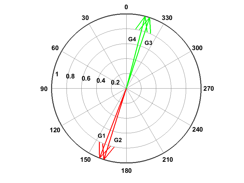
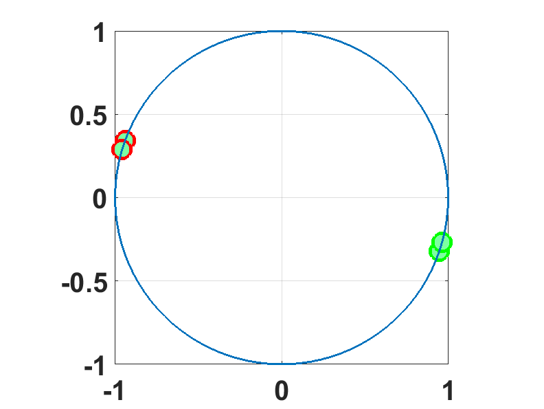
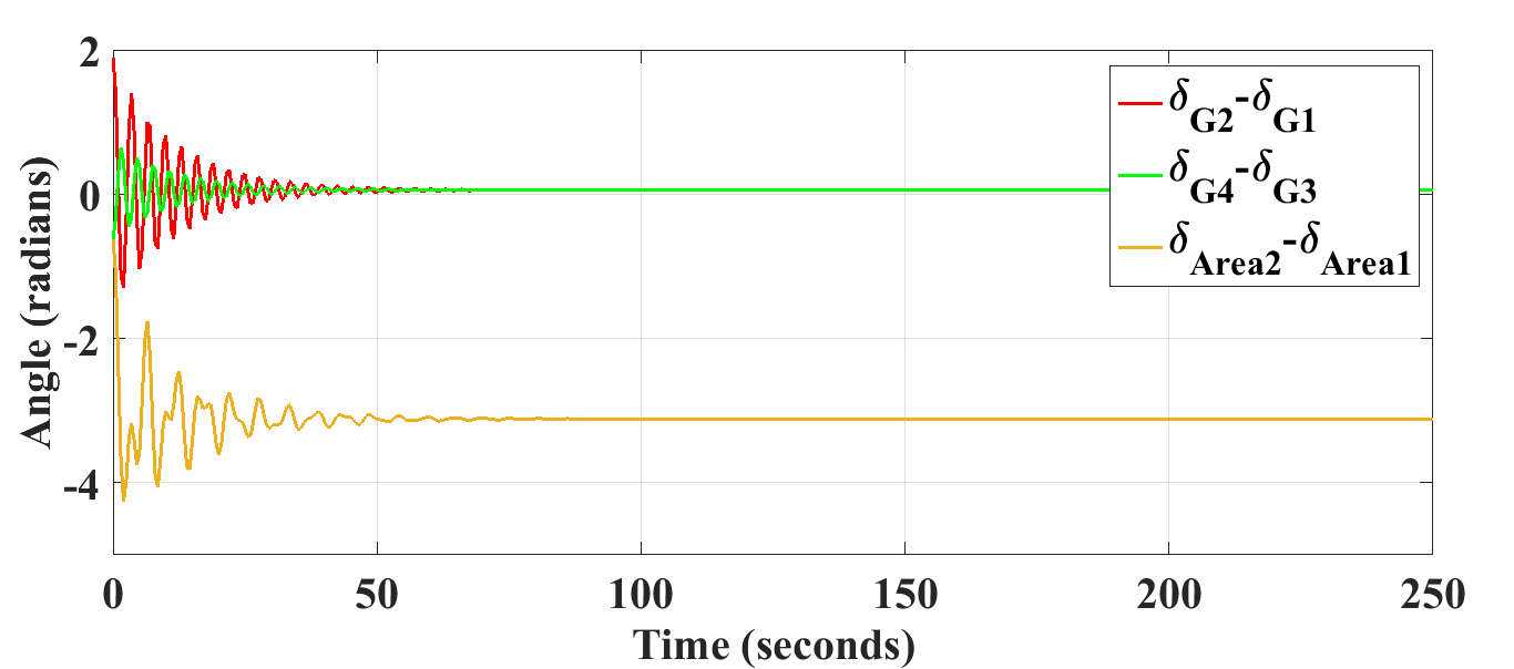
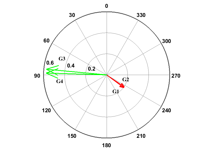
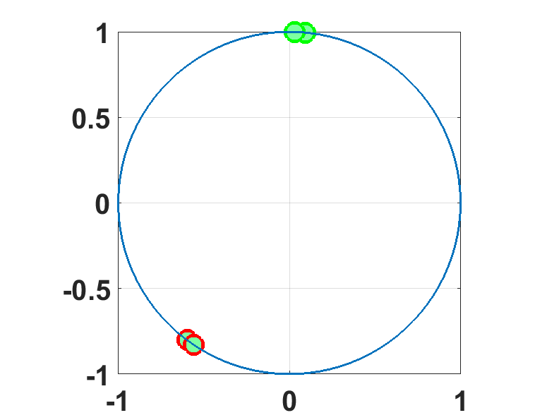
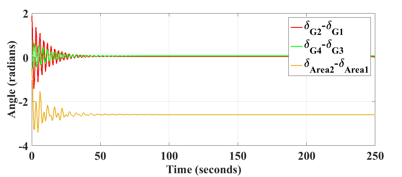
Case 1: The generators oscillate anti-phase ($-3.12\approx-\pi$radians) in interarea and in-phase ($0.06\approx 0$radians) intraarea. To validate the results, we provide compass plots of normalized eigen modes, circle plot as well as time-domain plots of generators as shown in Figure 3. The compass plots were obtained by using the steady-state vectors: $\vec{c}_{i}(t)=\big(\delta_{j}-\delta_{i}\big)_{rms}\angle\delta_{i}(t)\sim\big(\delta_{j}-\delta_{i}\big)_{rms}\left(\sum^{n}_{i=1}e^{\lambda_{i}t}u_{i}v^{T}_{i}\delta_{i}(0)\right)$, where $u_{i}$ is the normalized left eigen-vector, $v_{i}$ is the normalized right eigen-vector and $\lambda_{i}$ are the eigen-values of the linearized system. It can be seen that the compass plot of steady state vectors show behavior similar to normalized eigen modes obtained by small-signal analysis performed traditionally.

Case 2: In the case when power is transferred between areas, the phase difference between interarea generators were observed to be $-2.6$radians (i.e., $\neq-\pi$) and $0.05$radians in intraarea, as shown in Figure 3. The results are compared with [2], providing validity to the proposed model.

In power systems, the equal area criterion is a “graphical technique used to examine the transient stability of the machine systems (one or more than one) with an infinite bus". The areas under the curve of a power angle diagram are equated across to calculate effective acceleration/deceleration thereby comment on the stability of the system. For instance, consider (18), rewriting in terms of mechanical and electrical power interactions,

$$\ddot{\delta}_{i}=P_{m,i}-\hat{P}_{transmitted},$$

(21)

where $\hat{P}_{transmitted}=\alpha_{i}\dot{\delta_{i}}-P_{max}sin(\Delta\delta_{ij})=P_{transmitted}-P_{dissipated}$. It can be seen that the collective acceleration of generators is dependent on the difference of mechanical and electrical power inputs. As shown in Figure 4, difference in electrical-mechanical inputs either accelerate or decelerate the generators to achieve equilibrium. The generators accelerate when mechanical power is higher than the transmitted electrical power (i.e., $P_{m,i}>P_{transmitted}$) and decelerate when electrical power is higher (i.e., $P_{m,i}<P_{transmitted}$). This is due to the fact that, the difference in the power gives rise to the rate of change of accumulated power ($P_{accumulated}$) in the rotor masses. The change in accumulated power and generator inertia results in effective change in rotor angles, thereby acceleration/deceleration and vice-versa. The coupled set of generators happen to achieve steady-state, when mechanical power of the generator from turbines match the transmitted electrical power. This can be visualized as creation of a ‘sink’ node, where the system tries to drive itself in order to achieve stability. Thus, any generator starting from a rotor angle $\in[\delta_{0},\delta_{c},\delta_{m}]$, will try to move towards $\delta_{0}$ (or stability). On the other hand, $\delta_{m}$ happens to be critically stable and a small perturbation towards $\pi$ radians can render increase in rotor angles due to effective acceleration of generators. In such case, a ‘source’ node is formed at $\pi$ radians, as shown in Figure 4.

Generators are mechanical devices that exhibit high inertia and hence require time to achieve stability, once perturbed from its equilibrium. The natural speed (angular speed) of rotation $\omega_{i}$ and generator inertia $J$ along-with accumulated power $P_{accumulated}$ in turn defines the rate at which stability is achieved or if system becomes unstable. As shown in Figure 4, although $\omega_{i}$ and $J$ are constants if generator achieves stability via route 2 has higher $P_{accumulated}$ and is highly susceptible to instability as compared to route 1. We show this using circle plot and thereby its relevance to ‘$\pi$’, ‘transmitted’ and ‘incoherence’ state as mentioned in previous sections. Thus, it can be inferred that a ‘source’ node imparts instability whereas ‘sink’ node stabilizes a power setup. These inferences can be easily made using CC-Kuramoto model as these nodes are pretty evident. In the next section, we do a bifurcation analysis on CC-Kuramoto model in order to understand the effect of system parameters on system stability.

References

- [1] Graham Rogers. Power system oscillations. Springer Science & Business Media, 2012.
- [2] Meir Klein, Graham J Rogers, and Prabha Kundur. A fundamental study of inter-area oscillations in power systems. IEEE Transactions on power systems, 6(3):914–921, 1991.
- [3] Giovanni Filatrella, Arne Hejde Nielsen, and Niels Falsig Pedersen. Analysis of a power grid using a kuramoto-like model. The European Physical Journal B, 61(4):485–491, 2008.
- [4] Hyunsuk Hong and Steven H Strogatz. Kuramoto model of coupled oscillators with positive and negative coupling parameters: an example of conformist and contrarian oscillators. Physical Review Letters, 106(5):054102, 2011.
- [5] P Kundur and Lei Wang. Small signal stability analysis: experiences, achievements, and challenges. In Power System Technology, 2002. Proceedings. PowerCon 2002. International Conference on, volume 1, pages 6–12. IEEE, 2002.
- [6] Kwan-Shik Shim, Seon-Ju Ahn, and Joon-Ho Choi. Synchronization of low-frequency oscillation in power systems. Energies, 10(4):558, 2017.
- [7] DeTao Mao, Peng Zhang, Hafiz Abdur Rahman, and Jose R Marti. Nonlinear oscillations caused by periodic disturbance between inter-area power systems. In Electric Power Conference, 2008. EPEC 2008. IEEE Canada, pages 1–5. IEEE, 2008.
- [8] Daniel M Abrams and Steven H Strogatz. Chimera states for coupled oscillators. Physical review letters, 93(17):174102, 2004.
- [9] North American Electric Reliability Corporation. Nerc system disturbances reports. 1992-2009.
- [10] Yoshihiko Susuki and Igor Mezic. Nonlinear koopman modes and coherency identification of coupled swing dynamics. IEEE Transactions on Power Systems, 26(4):1894–1904, 2011.
- [11] Yoshihiko Susuki, Igor Mezic, and Takashi Hikihara. Global swing instability in the new england power grid model. In 2009 American Control Conference, pages 3446–3451. IEEE, 2009.
- [12] Pablo A Parrilo, Sanjay Lall, Fernando Paganini, George C Verghese, Bernard C Lesieutre, and Jerrold E Marsden. Model reduction for analysis of cascading failures in power systems. In Proceedings of the 1999 American Control Conference (Cat. No. 99CH36251), volume 6, pages 4208–4212. IEEE, 1999.
- [13] Florian Dorfler and Francesco Bullo. Synchronization and transient stability in power networks and nonuniform kuramoto oscillators. SIAM Journal on Control and Optimization, 50(3):1616–1642, 2012.
- [14] Florian Dörfler and Francesco Bullo. On the critical coupling for kuramoto oscillators. SIAM Journal on Applied Dynamical Systems, 10(3):1070–1099, 2011.
- [15] Adilson E Motter, Seth A Myers, Marian Anghel, and Takashi Nishikawa. Spontaneous synchrony in power-grid networks. Nature Physics, 9(3):191, 2013.
- [16] Richard P Feynman, Robert B Leighton, and Matthew Sands. The Feynman lectures on physics, Vol. I: The new millennium edition: mainly mechanics, radiation, and heat, volume 1. Basic books, 2011.
- [17] Matthew Bennett, Michael F Schatz, Heidi Rockwood, and Kurt Wiesenfeld. Huygens’s clocks. Proceedings: Mathematics, Physical and Engineering Sciences, pages 563–579, 2002.
- [18] Priyanka Dey, Rachit Mehra, Faruk Kazi, Sushama Wagh, and Navdeep M Singh. Impact of topology on the propagation of cascading failure in power grid. IEEE Transactions on Smart Grid, 7(4):1970–1978, 2016.