Extracting galaxy merger timescales I: Tracking haloes with WhereWolf and spinning orbits with OrbWeaver 2019Extracting galaxy merger timescales I: Tracking haloes with WhereWolf and spinning orbits with OrbWeaver–C
Abstract
Hierarchical models of structure formation predict that dark matter halo assembly histories are characterised by episodic mergers and interactions with other haloes. An accurate description of this process will provide insights into the dynamical evolution of haloes and the galaxies that reside in them. Using large cosmological -body simulations, we characterise halo orbits to study the interactions between substructure haloes and their hosts, and how different evolutionary histories map to different classes of orbits. We use two new software tools - WhereWolf, which uses halo group catalogues and merger trees to ensure that haloes are tracked accurately in dense environments, and OrbWeaver, which quantifies each halo’s orbital parameters. We demonstrate how WhereWolf improves the accuracy of halo merger trees, and we use OrbWeaver to quantify orbits of haloes. We assess how well analytical prescriptions for the merger timescale from the literature compare to measured merger timescales from our simulations and find that existing prescriptions perform well, provided the ratio of substructure-to-host mass is not too small. In the limit of small substructure-to-host mass ratio, we find that the prescriptions can overestimate the merger timescales substantially, such that haloes are predicted to survive well beyond the end of the simulation. This work highlights the need for a revised analytical prescription for the merger timescale that more accurately accounts for processes such as catastrophic tidal disruption.
Keywords:
methods: numerical – galaxies: evolution – galaxies: haloes – dark matter1 Introduction
In the standard cosmological model, dark matter haloes grow hierarchically, whereby low mass haloes merge to build up progressively more massive systems. Some of these merged systems survive as substructure haloes or subhaloes (Tormen 1997; Tormen et al. 1998; Klypin et al. 1999; Moore et al. 1999, e.g.), and can exist for long periods within their host, undergoing many orbits (Boylan-Kolchin et al. 2008; Jiang et al. 2014, e.g.). The manner in which a subhalo is accreted can change drastically subsequent evolution of both the subhalo and its host halo (White & Rees 1978; Blumenthal et al. 1986; Dubinski 1994; Mo et al. 1998, e.g.). A subhalo will continue to orbit within its host until it either (1) merges with the host, or (2) is tidally disrupted as a result of mass loss driven by tidal heating and stripping (Ostriker et al. 1972; Gnedin et al. 1999; Dekel et al. 2003; Taylor & Babul 2004; D’Onghia et al. 2010, e.g.). If the subhalo hosts a satellite galaxy but undergoes tidal disruption, then the satellite can persist even after the subhalo’s disruption (Springel et al. 2001; Kravtsov et al. 2004; Zentner et al. 2005; Conroy et al. 2006; Natarajan et al. 2009, e.g.). The eventual fate of the satellite depends strongly on the type of orbit it was on when its host (sub)halo was lost. Galaxies on highly circular orbits can survive longer than those on radial orbits, and so can have a strong influence on the galaxy merger rate and how galaxy mergers happen (Wetzel 2011).
The merger rate depends on the dynamical friction timescale, and the dependence of this timescale on the orbit of the merging system has been modelled extensively (Binney & Tremaine 1987; Lacey & Cole 1993; Jiang et al. 2008; Boylan-Kolchin et al. 2008; Simha & Cole 2017, e.g.). These merger timescale prescriptions are used in Semi-Analytical Models (SAMs) to estimate a satellite galaxy’s survival time, i.e. determine when it will merge with its host halo (Lacey & Cole 1993; Cora et al. 1997; Fujii et al. 2006; Jiang et al. 2008; Boylan-Kolchin et al. 2008; Jiang et al. 2014; Simha & Cole 2017; Lagos et al. 2018, e.g.). These prescriptions are of vital importance when coupling SAMs to large volume cosmological -body simulations, which do not have either the mass or snapshot resolution to allow subhaloes to be accurately tracked to the point at which they disrupt and the galaxy merges.
To ensure that estimates for the merger timescale are accurate, high spatial and temporal resolution simulations are used to calibrate the timescale by tracking subhaloes until they have complete disrupted and they are deemed to have merged. However, even with high resolution, tracking subhaloes is a challenging problem. In cosmological simulations, (sub)haloes can disappear and then re-appear, sometimes multiple times, in consecutive halo catalogues, especially when they are in dense environments, which can lead to estimates of premature merging and artificially reduced merger timescales (Poulton et al. 2018; Elahi et al. 2019b).
In this work, we present two new open source software tools - WhereWolf11 1 https://github.com/rhyspoulton/WhereWolf and OrbWeaver22 2 https://github.com/rhyspoulton/OrbWeaver. WhereWolf is a (sub)halo ghosting tool, which is used to track (sub)haloes even after they have been lost by the halo finder, and to supplement halo catalogues with these recovered (sub)haloes. We show how using WhereWolf can improve measurements of the subhalo/halo mass function, and present estimates of the distribution of radii at which subhaloes merge. OrbWeaver, extracts orbital properties, such as eccentricity and orbital energy, at key points in a subhalo’s orbit. We show the distribution of orbital properties recovered by OrbWeaver, and we compare our results to previous work. Finally, we show how current prescriptions of the merger timescale from Binney & Tremaine 1987; Lacey & Cole 1993; Jiang et al. 2008; Boylan-Kolchin et al. 2008 perform on the latest generation of large N-body simulations.
This paper is organised as follows: in §2 we discuss the data and the codes used; our results on constructing halo orbits are presented in §3; orbital analysis of (sub)haloes is presented in §4; and in §5 we conclude the paper with a discussion on the importance of accurate halo tracking in simulations.
2 Input Catalogues
The simulations used in this work come from two suites of -body simulations; (1) genesis (Elahi et at., in preparation), with volumes ranging from 26.25 to 500 Mpc and between 3243 to 43203 particles; and (2) SURFS (Synthetic UniveRses for Future Surveys) (Elahi et al. 2018), with volumes ranging from 40 to 900 Mpc and between 5123 to 20483 particles. Both suites of simulations were run assuming a CDM Planck 2015 cosmology with = 0.3121, = 0.6879, = 0.6879, a normalisation = 0.815, a primordial spectral index = 0.9653, and a (Alves et al. 2016). A total 200 snapshots are stored, evenly spaced in logarithmic expansion factor () between to . This high cadence enables an accurate capturing of the evolution of dark matter haloes and their orbits. Both suites of simulations have been run with a memory-lean version of GADGET2 (Springel et al. 2005)
For this study, we focus on the genesis simulation, with a box size of 105 Mpc and 20483 particles, implying a particle mass of 1.73 M⊙; and the SURFS simulation, with a box size of 40 Mpc and 5123particles, with a particle mass of 4.12 M⊙. These boxes provide us with a statistical sample of well resolved central haloes, with virial masses 1010.5M⊙; at least 1,000 particles for centrals, and at least 20 particles for subhaloes. Unless otherwise stated, we use genesis volume for our analysis.
Halo catalogues are constructed using VELOCIraptor a 6-Dimensional Friends-of-Friends (6D-FoF) phase space halo finder (Elahi et al. 2011; Elahi et al. 2013; Cañas et al. 2019; Elahi et al. 2019a), while trees are constructed using TreeFrog (Elahi et al. 2019b), which is a particle correlator that can link across multiple snapshots and halo catalogues. Importantly, TreeFrog’s ability to link across multiple snapshots is vital for tracking subhaloes as they orbit within highly overdense regions. While a subhalo may not be present in a pair of halo catalogues at consecutive output times, it may be present in halo catalogues at a later time, and so there might be gaps in the subhalo’s history. This has led to the development of the halo tracking tool known as WhereWolf.
2.1 WhereWolf

WhereWolf is a (sub)halo tracking tool, originally introduced in Poulton et al. 2018. A representation of the WhereWolf decision tree is shown in Figure 1. In summary, (sub)haloes are identified by gaps in TreeFrog trees, and their particles are extracted from a VELOCIraptor catalogue and propagated forward in time to see if these (sub)haloes remain bound at later times, or if they have been permanently disrupted. There are two cases in which WhereWolf is triggered:
1. a (sub)halo has a descendant that is more than one snapshot away, which can occur during TreeFrog multi-snapshot linking;
2. two (sub)haloes merge, and a (sub)halo’s descendant becomes ambiguous.
A schematic of the above two cases is shown in Figure 2. In both cases, WhereWolf tracks a (sub)halo if Npart > Nmin,track, where Nmin,track is the minimum particle number. For this paper, Nmin,track is set to 50 particles because this is above the 20 particle limit for a (sub)halo to exist in the catalogue and to be tracked for at least one snapshot (boxes 1 and 2 in Figure 1).
2.1.1 WhereWolf in Depth
In this Section we explain how WhereWolf works in detail.
1. Boundedness calculation. WhereWolf estimates the boundedness of a (sub)halo by calculating the escape velocity (Vesc) profile, which can be related to the circular velocity by: . Assuming a Navarro Frenk and White profile33 3 We use a theoretical model to calculate Vcirc because direct measurement from the simulation can be noisy, especially at small radii where there is little enclosed mass. Also, because is being calculated for subhaloes, the particles at large radii are also subject to the effects of the host. Hence by using the theoretical model, we can use more stable quantities e.g. Mvir, Rvir and c. Here the concentration is evaluated by assuming the last value that was measured by VELOCIraptor. (Navarro et al. 2002, NFW;), Vcirc is given by:
| (1) |
here = is the concentration, where is the scale radius and is the virial radius, defined such the mean interior density = 200. The function is given by
| (2) |
with = . Vvir is calculated as,
| (3) |
where is the gravitational constant in relevant units, and is the mass of the (sub)halo contained within (box 3 in Figure 1). Particles are considered bound if they are below Vesc and are with Rvir.

2. Tagging candidate tracked (sub)halo particles. In the initial snapshot at which tracking begins, and are taken from the VELOCIraptor catalogue. From this, WhereWolf determines whether or not a particle is bound to the (sub)halo using the above binding conditions. An example candidate (sub)halo is shown in Figure 3, where the shaded region indicates which particles are bound to it. The most bound particles (MBPs) are determined by calculating the following distance metric for all particles:
| (4) |
where and are the relative position and velocity of the (sub)halo to its centre of mass. This metric is used to find the MBPs, where the minimum 10% are defined as the MBPs, with a minimum of 10 MBPs (box 4 in figure 1).
3. Following tracked (sub)halo particles. The MBPs in the example shown in Figure 3 are indicated by red points; these populate the core of the caustic and are used to determine reference positions and velocities for the tracked (sub)halo at the next snapshot (box 9 in Figure 1). WhereWolf estimates and from the MBPs by finding the radius at which the enclosed density drops below 200.
At this point, is re-calculated to find which particles belong to the (sub)halo (boxes 10 and 3 in Figure 1), along with re-calculating the MBPs (box 4 in Figure 1). Only particles within 10 times the mean radius are retained; this is because particles can move large distances between snapshots and become completely unbound from the (sub)halo. If there are fewer than 20 bound particles, then the (sub)halo is not tracked forward to the next snapshot (boxes 5 and 11 in Figure 1), otherwise, an attempt is made to identify the (sub)halo in the VELOCIraptor catalogue (box 6 in Figure 1). This is done using a K-D tree (Bentley 1975) to find (sub)haloes that fall within the tracked (sub)halo’s , and a (sub)halo is matched to the tracked (sub)halo if and only if it does not have a progenitor, i.e. the (sub)halo’s branch is truncated. This reduces the number of truncated branches and avoids terminating a branch when it does not have a descendant, which would happen when a non-truncated branch is matched. In this situation the WhereWolf connection would overwrite the TreeFrog connection, meaning that a (sub)halo that was previously connected would not have a descendant.
Matching is achieved by comparing particles that belong to each (sub)halo and using a merit function44 4 For details on the full merit functions that are used, please see (Elahi et al. 2019b)., such as,
| (5) |
here is the number of particles shared between two (sub)haloes; is the number of particles in the WhereWolf (sub)halo; and is the number of particles in the matched VELOCIraptor (sub)halo. A match occurs when >0.025, and the descendant for the tracked (sub)halo points to the matched VELOCIraptor (sub)halo. We can also apply the same merit to the MBPs using the same threshold.
If a match is not found, (sub)haloes that are within the tracked (sub)halo’s are used to identify if the WhereWolf (sub)halo stays within 0.1 Rvir of a VELOCIraptor (sub)halo for more than 3 snapshots; if so, the WhereWolf (sub)halo is considered completely merged with the VELOCIraptor (sub)halo. This removes any (sub)haloes that remain bound, even after they have merged formally, and avoids (sub)haloes persisting for many snapshots (box 6 in Figure 1).
If no match is found and the tracked (sub)halo has not remained within 0.1 Rvir of a VELOCIraptor (sub)halo then the tracked (sub)halo is "accepted" and WhereWolf determines if the tracked (sub)halo has a host. The host of a WhereWolf (sub)halo is determined by checking if the initial VELOCIraptor (sub)halo (which was used to identify the WhereWolf (sub)halo) has a host. If a host exists, then the WhereWolf (sub)halo is set as a descendant if it exists in the next snapshot. If there is no host for the initial VELOCIraptor (sub)halo or if it does not exist in the next snapshot, a search is carried out to determine if the (sub)halo has a new host. This is done by checking if the WhereWolf (sub)halo lies within the Rvir of a VELOCIraptor halo using the K-D tree, and then checking if it is bound to the halo by evaluating
| (6) |
where is the virial mass of the WhereWolf (sub)halo; is the velocity of the WhereWolf (sub)halo relative to the VELOCIraptor halo; is the virial velocity of the VELOCIraptor halo; and |rWW - rVEL| is the separation between the WhereWolf and VELOCIraptor haloes. Equation 6 establishes whether or not the WhereWolf halo is bound to the VELOCIraptor halo (box 7 in Figure 1). If the WhereWolf (sub)halo can be tracked, it is added to the VELOCIraptor halo catalogue (box 8 in Figure 1).
It is clear that adding in these (sub)haloes will impact the reconstruction of subhalo orbits. We can study the impact of WhereWolf on our orbital reconstruction using our newly developed orbital analysis tool, which is known as OrbWeaver. This is introduced and discussed in detail in the next Section.
2.2 OrbWeaver
OrbWeaver is a tool for processing merger trees and extracting orbital catalogues for a statistical sample of (sub)haloes from cosmological simulations. A representation of how OrbWeaver works is shown in Figure 4. In summary, for each halo in a VELOCIraptor catalogue, OrbWeaver tracks the full histories of all other (sub)haloes that have passed within N Rvir (where N is a positive integer) of the host of interest (Rvir,host) across cosmic time (boxes 1, 2 and 3 in Figure 4).
Once processed, (sub)haloes are assigned OrbitIDs55 5 A given (sub)halo can have multiple OrbitIDs. and written to catalogue (box 4 in Figure 4). In this way, every (sub)halo that satisfies a given OrbitIDs can be extracted, and the orbital properties – a list of which is given in Appendix – of this set are recorded at two points:
- •
the crossing point, at which the (sub)halo crosses times the host virial radius (Rvir,host) with ; and
- •
the apsis point, at which a (sub)halo’s radial velocity vector (Vrad) changes direction. If the radial velocity goes from negative to positive, it is a peri-centric apsis, otherwise it is an apo-centric apsis.
A root finding algorithm is used to find the crossing and apsis points so that (sub)halo properties – position, velocity, mass, maximum circular velocity (Vmax), and virial radius – are interpolated to the exact point that the event happens (box 5 in Figure 4). Most orbital properties are calculated at both points, but there are some properties (such as eccentricity ()) that are calculated only for apsis points. The table in Appendix explicitly states when each property is computed.
2.2.1 Orbit cleaning
Once orbits have been processed they are cleaned to remove duplicate crossing points or spurious apsis points (box 6 in Figure 4).
- •
Duplicate crossing points arise because of fluctuations in Rvir,host. The orbiting (sub)halo can be within the Rvir,host in one snapshot, but outside in the next because Rvir,host has shrunk, and so it appears to have crossed Rvir,host twice. These duplicate crossing points are removed by storing only the first instance of the infall crossing point and only storing further crossing point once the (sub)halo has had a least one outgoing crossing point. This means that the orbiting (sub)halo is set to cross Rvir,host only once, at first infall, and must have an outgoing crossing point before it infalls again.
- •
Spurious apsis points arise because the orbiting (sub)halo can interact with other orbiting (sub)haloes, which can cause perturbations in its orbit; it can also occur when the (sub)halo is part of a larger, infalling, group. In both cases, the orbiting (sub)halo can experience large changes in Vrad as well as brief changes in its direction, which can lead to it being classified as having had a apsis point about the halo it is orbiting.
An example spurious apsis point is shown in Figure 5, which shows properties of a (sub)halo as it orbits its host. The red circle highlights the occurrence of a incorrectly identified apsis point based on when the radial velocity changes direction. This is caused by the large change in the relative velocity (Vrel), which occurs because of the orbiting (sub)halo gravitationally interacting with another, similar mass, subhalo at this snapshot. This interaction is cleaned by discarding any apsides that happen within two snapshots, as the orbit will not have been adequately sampled.

3 Results
3.1 WhereWolf: Halo Mass Functions & Merging Radii, Rmerge

We begin by showing halo mass functions (HMF) and subhalo66 6 By subhalo here we mean a halo that is not the top of its spatial hierarchy mass functions (SHMF) in Figure 6, where we have used the 1053 Mpc box with 20483 particles. The top left panel shows the HMF , while the top right panel shows the SHMF for WhereWolf (dashed orange line) and VELOCIraptor (solid blue line). Most of the subhaloes and haloes populated by WhereWolf are at masses and respectively, which reflects the greater likelihood that lower mass (sub)haloes are more likely to be lost by VELOCIraptor and to be picked up by WhereWolfś tracking. The power-law slopes of the respective HMF and SHMF at these low masses are in reasonable agreement. The bottom panel of 6, shows the relative difference between the catalogues HMF (solid line) and SHMF (dashed line). This demonstrates that WhereWolf identifies an increased number of subhaloes in the catalogue, where the difference can be as high as 15% in some mass bins with an average increase of 10% more subhaloes than VELOCIraptor. In comparison, WhereWolf does not track many haloes whereby the increase in the number of haloes is <1% . This shows that the integration of the WhereWolf haloes into the VELOCIraptor catalogues does not have an effect on the shape and amplitude of the HMF derived from the VELOCIraptor catalogue, which is shown to be in good agreement with various HMFs such as (Tinker et al. 2010) shown in the top panel of Figure 6 (see (Elahi et al. 2018) for other mass functions).
In Figure 7 we show the probability distribution function (PDF) of the radii at which subhaloes merge with their hosts (Rmerge), estimated from the original VELOCIraptor catalogues (heavy dark solid histogram) and the revised VELOCIraptor + WhereWolf catalogues (heavy light solid histogram). This demonstrates that WhereWolf tracks subhaloes to smaller radii before they merge, while also extending the temporal baseline over which we can track subhaloes and characterise their orbital properties. This highlights that WhereWolf improves tracking of lower mass haloes and subhaloes, which are the most susceptible to being lost in any halo finding algorithm, and allows their orbits to tracked for longer and into higher overdensity regions.

3.2 OrbWeaver: Orbital Parameters

OrbWeaver computes a multitude of properties that characterise the orbits of subhaloes around their host haloes. For this paper we focus on a few key properties, such as circularity () defined as
| (7) |
where is the specific angular momentum of the orbiting (sub)halo and is the specific angular momentum of the equivalent circular orbit with the same energy (E); both of these quantities are calculated at first infall (i.e. when the subhalo first crosses Rvir,host). The distribution of is shown in Figure 8 for all (sub)haloes at that had at least 1,000 particles at infall, corresponding to a mass of 1.5 M⊙. This distribution is broad and peaks at , which is in good agreement with previous work (Tormen 1997; Zentner et al. 2005; Wang et al. 2005; Khochfar & Burkert 2006; Jiang et al. 2008; Wetzel 2011; Jiang et al. 2015; van den Bosch 2017), and shows that most satellite orbits are neither preferentially circular nor highly radial.
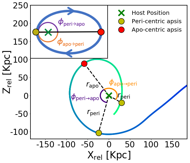
We also study eccentricity of the orbit () and angle subtended since last apsis of an orbiting subhalo relative to the host halo (). Here 77 7 We refer the reader to Appendix C for discussion about the meaning of the physical meaning of . is computed as
| (8) |
where nd are apo- and peri-centric distances respectively. Figure 9 shows a visual representation of how and are calculated.


Figures 10 and 11 show the and distributions for peri-centric and apo-centric apsides respectively. These Figures show that apo-centric apsides happen at smaller than peri-centric apsides do, which, as we argue in § 3.3.2, occurs because most subhaloes are on in-spiralling orbits. Peri-centres, however, have a of close to 180∘ with respect to the previous apo-centre; this is because (sub)haloes experience most of their mass loss at peri-centre, with a correspondingly large change in angular momentum. This means that subhaloes transition to lower energy orbits with smaller apo-centres, which continues until the subhalo disrupts and is merged with the host.

A striking feature of both Figure 10 and Figure 11 is that there are two populations, which can be seen clearly in the right histograms. Both Figures have a second population at low and . To understand this further, we plot an example orbit with of 17∘ and ; this is shown in Figure 12, where it can be seen that these apses are due to the (sub)halo interacting with another orbiting (sub)halo of a larger mass. The interaction causes it to undergo changes in radial velocity over a narrow radial range and to have apses close together, which results in small and . This is the effect described previously in Section 2.2.1 and shown in Figure 5, but because it happens over a longer timescale, it is not removed by the initial clean.
From Figure 11, it is clear that such interaction-induced low values of and are more likely to happen when a peri-centre is followed by an apo-centre. This is because most interactions involve a less massive subhalo orbiting its more massive host, and because the orbit of the more massive subhalo will be relatively unperturbed, it is the less massive subhalo that will first experience an outward apsis point (Vrad>0) relative to the host halo, followed by an inward apsis point (Vrad<0), thereby resulting in repeated peri- and apo-centres. These false apsides typically happen at larger radii where the orbiting subhalo is more likely to interact with other orbiting subhaloes.

To better understand where these orbital wobbles occur, we plot a 2D histogram of and but colour-code by the mean smallest radius of closest approach, RCA (the closest the subhalo has been to its host up to this point), along each (sub)halo’s orbit, normalised by Rvir,host in each bin; this is shown in Figure 13. The top panel shows and for apo-centre to peri-centre; the lower panel shows peri-centre to apo-centre. In the top panel, it can be seen that orbits that tend to have a of 180∘ and high have a very small value of RCA at peri-centre, as expected. False apsides at low and tend to have a large value of RCA for their closest approach, typically outside Rvir,host.

The population of orbits that wobble are clearly shown in Figure 14, which is the similar to Figure 13 but is colour-coded by the mean ratio of measured to Keplerian orbital periods in each bin ( and respectively), where,
| (9) |
where is the semi-major axis, is the mass of the orbiting subhalo, and is the mass of the host halo (Russell 1964). Figure 14 clearly shows that the apsides that have low ratios of are orbits with low and . These apsides are, in fact, merely orbital wobbles, and lead to a low period because they happen over a short time, as can be seen in Figure 12.

From Figure 11, there is a less apparent third population which has high but low . This population becomes more apparent when points on the figure are colour-coded by the radius of current closest approach in each (sub)halo’s orbit () normalised to , as shown in Figure 13. There is a clear trend in the apo-centres, where apo-centres with low and tend to have large values of , while those with high and low tend to have smaller values of .
To better understand this, we show in Figure 15 an example orbit drawn from this region. We see that the orbiting subhalo has a very radial orbit, in which it passes very close to its host and undergoes a quick change in direction of . Because it passes so close to its host, the orbiting (sub)halo loses a lot of angular momentum and is unable to maintain its orbit. This causes the (sub)halo to undergo a rapid change in velocity, and it quickly merges with its host. This apsis has a low because the (sub)halo could not complete a full orbit, but has a high value of since its first apsis is close to its host, but its secondary apsis happens at larger radius.
3.3 Toy Orbital Evolution Model
To understand why there is a difference in at peri- and apo-centres, we model a subhalo orbiting in a NFW halo with a potential given by
| (10) |
where is the host halo-centric radius; = Rvir/ is the scale radius, where is the concentration of the halo; is the critical density; and is the characteristic overdensity given by
| (11) |
We assume that the density profile is truncated just outside . The orbit is calculated in 2-dimensions over a time of 1 Gyr; a order leapfrog integrator is used with 1,000 steps equally spaced in time (i.e. 1 Myr). The initial conditions are and , where is the virial velocity of the host halo.
3.3.1 A simple model
As our starting point, let us assume that (1) the only force acting on the subhalo is the gravity of the host halo; (2) the subhalo can be treated as a point particle with negligible relative mass; (3) the mass of the host does not change in time, and (4) its density profile is fixed; and (5) the orbital angular momentum of the subhalo is constant. The results of our model using these assumptions are shown in Figure 16. It can be seen that angles between the apsides - shown by the cyan, green, yellow and purple lines - are always below 180∘; in other words, an orbit in a NFW potential causes apsidal procession. In the case of the toy orbit shown in Figure 16, the angle between the apsides is a constant 130∘. While this model explains why can be below 180∘, it does not explain the differences in found at peri-centre and apo-centre, as seen in Figures 10 and 11.

3.3.2 A more complex model
We now relax assumption (3), which is that the mass of the host halo is constant, and allow it to increase with time by a factor of 3 over the period of the orbit; this was found to be a typical value for mass change over 1 Gyr. We also increase the concentration of the host, , by a factor of 2 over the same period. In addition, we relax assumption (5) and assume that the subhalo loses some orbital angular momentum (Lorb) at peri-centre, as would occur if the subhalo was disrupted. Results of this more complex model are shown in Figure 17. The increase in the mass of the host and the loss of Lorb causes the angle between peri- and apo-centre (cyan and purple angles) to be smaller than in the simple model - with fixed host mass and constant angular momentum - and close to 90∘. In addition, the angle between apo- and peri-center (green and yellow angles) is close to 180∘, which is seen in Figures 10, 11 14 and 13.
We now investigate which property has the most significant effect on – Mhost increasing, chost increasing or Lorb.


Increasing Mhost
Here we assess the impact of increasing of Mhost by contrasting in models in which Mhost is increasing with ones in which it is fixed (). We systematically vary the initial conditions, exploring a range of values in both models; initial positions are required to be outside a radius of 0.5 Mpc, while velocities are required to be below the escape velocity of the host at the initial position and greater than 0.3Vvir 88 8 This ensure that the halo orbits its host and does not merge on a short timescale..
We plot the PDF and medians of as measured when the halo has completed three peri-centric and apo-centric apsides in the upper panels of Figure 18; left and right panels show the cases when the subhalo passes from apo- to peri-centre (Apo-Peri) and peri- to apo-centre (Peri-Apo) respectively. Line colour indicates the number of apsides completed, where three of each apsis is shown. This shows that increasing Mhost causes to decrease, and for the magnitude of the decrease to increase with each apsis. This is because increasing Mhost reduces the relative orbital energy of the satellite, meaning that its orbital speed around the host is decreased and so apsis occurs more quickly. The effect is more pronounced when going from Peri-Apo, which is most likely because orbits will experience a peri-centre first, and it is post- first peri-centric passage when they lose most of their orbital energy.
Increasing chost
Here we assess the impact of increasing the host NFW profile concentration (chost), following the approach used in the previous sub-Section. We keep the enclosed mass at the truncation radius fixed. The middle panels of Figure 18 shows, as before, the PDF of the difference of this model’s to the simple model . In contrast to the case of increasing Mhost, we see that increasing chost leads to a corresponding increase in the angle when going from peri- to apo-centre (). This is because increasing chost means that Mencl is always higher after apsis than before it. We expect that this increase will be minimal after peri-centre because this is when the orbiting halo is travelling the fastest, but it should be more pronounced after apo-centre, when Vrad < 0. The subhalo’s speed will increase, resulting in a shorter orbital time, and a corresponding increase in .
Decreasing Lorb
Finally, we assess the impact of decreasing Lorb. This decrease occurs at peri-centre, where the average Lorb decrease is estimated from the -body simulation. The PDF of for this is shown in the bottom panels of Figure 18, where we observe that decreasing Lorb generally leads to lower . As with increasing , the subhalo loses orbital energy, which means that it takes longer to complete an orbit, which leads to a decrease in . However, we find that this decrease in Lorb has a negligible effect. This may be because of the simplified treatment in our model, e.g. we neglect dynamical friction, which might be important in this regime for some subhaloes, particularly for subhaloes which are on semi-stable orbits. A more sophisticated treatment is beyond the scope of this paper.
The net effect
Considering all the results shown in Figure 18, we conclude that Apo-Peri increases with the number of orbits because of the increase in Chost, whereas Peri-Apo decreases because of the increase in Mhost. The overall affect is that increases for Apo-Peri and decrease for Peri-Apo, which is seen to happen in Figure 17. The net effect is also what is observed to happen to the example planar orbit in Figure 9, where > . The model presented here offers a reasonable explanation of the effect observed.
3.4 Orbit Cleaning
Any automated approach to classifying orbits must account for wobbles in a subhalo’s orbit. As discussed above, these may arise because of interactions with other subhaloes. After investigation, we suggest cleaning apsides that satisfy the following criteria:
| (12) |
To show the effect of removing false peri/apo-centres (i.e. those that satisfy these criteria) on the distribution of orbital periods, we plot apsis radii (Rapsis) measured relative to Rvir,host and in Figure 19. We contrast the pre-cleaned distribution of peri- and apo-centres with the true, post-cleaned, and false, removed, distributions using criteria 12. This shows that false peri- and apo-centres generally have very short periods - with a mean of 1.4 Gyr - which is because apsides occur within a small time period. In contrast, the distribution of true apo- and peri-centres is much broader, with a mean of 2.8 Gyrs. The Rapsis ratio distribution for the false peri-centres (apo-centres) peaks outside of Rvir,host (3 Rvir,host), showing that these happen outside of the host and can be due to the subhalo orbiting another host as it comes in to merge with the host of interest. However, the defining property of false apsides is because peri- and apo-centres occur at similar radii.
We can see the effect of this cleaning on the orbital parameters in Figure 19, where we show PDFs of the orbital period; the radius of apsis (Rapsis) to Rvir,host; and . We indicate pre-cleaned, true post-cleaned, and false post-cleaned PDFs by solid, dashed, and dotted curves.
- •
Distribution of periods (left hand panel): we see that false apsides have a mean period of 1 Gyrs and a narrower distribution that tails off quickly at long periods, whereas true apsides have a mean period of 2 Gyrs, and a broad distribution with a long tail at long periods.
- •
Distributions of Rapsis/Rvir,host (middle panel): we see that false peri- and apo-centres peak at radii of approximately 1 times and 2 times Rvir,host, respectively, whereas the true peri- and apo-centres peak at 0.2 and 1 Rvir,host, respectively, with 99% of the peri-centres (apo-centres) lying within 1 (2) Rvir,host. This is in agreement with previous work (Khochfar & Burkert 2006; Ludlow et al. 2009; Barber et al. 2014, e.g.) .
- •
Distribution of (right hand panel): the false apsis points have a distribution that peaks sharply at < 0.2, as we would expect because of the small radial separation between the apsides for false orbits, whereas the distribution of true apsis points has a , which is consistent with (Barber et al. 2014)99 9 This distribution is based on the orbits of surviving z=0 subhalos of Milky Way mass halos using the N-body Aquarius simulations. Differences between our results and theirs may be due to the stricter orbit selection used in Barber et al. 2014 and the choice of MW mass hosts. However, since dark matter haloes are roughly self-similar, we expect the orbits to be roughly self-similar and difference to be small..
Figure 20 shows the PDF of the number of orbits that (sub)haloes experience after cleaning, where both the mean and median are shown to have a value of approximately 1. The PDF falls off as e, which suggests that most infalling (sub)haloes are on plunging radial orbits and complete only one orbit before they are disrupted. This agrees with the PDF (right-hand panel in Figure 19), where most orbits have a close to 1 and so are on more elliptical/ radial orbits. These type of orbits bring them close to their host, leading to a rapid mass loss. Consequently the (sub)halo is only able to survive for a single orbit.

3.5 Effect on the Merger Timescale

.
The merger timescale, i.e. the time from entering Rvir,host to the coalescence of the subhalo and the host halo, is strongly influenced by the type of orbit the subhalo is on. Many studies have looked into this effect and tried to quantify it (Binney & Tremaine 1987; Lacey & Cole 1993; Jiang et al. 2008; Boylan-Kolchin et al. 2008; Simha & Cole 2017, e.g.). Here we assess the prescriptions presented in Binney & Tremaine 1987 (hereafter BT87); Lacey & Cole 1993 (hereafter L93); Jiang et al. 2008 (hereafter J08); and Boylan-Kolchin et al. 2008 (hereafter BK08), and compare these prescriptions’ predictions with measurements from -body simulations in Figure 21. The panels show the measured merger timescales plotted against the merger timescales predicted by BT87 and L93 (upper left and right) and by J08 and BK08 (lower left and right). The red curves and shaded regions indicate medians and standard deviations for all of the haloes in our simulations.
Note that because the J08 and BK08 prescriptions are derived from -body simulations, we take care to apply the same selection criteria to our sample of haloes; the J08 criteria are:
| (13) |
While the BK08 criteria are:
| (14) |
These criteria define the subset of haloes for which medians (green curves) and standard deviations (shaded regions) are estimated in the lower panels of Figure 21.
We highlight the subset of (sub)haloes that are likely to have undergone artificial disruption (black triangles), which we exclude when calculating medians and standard deviations. The primary cause of artificial disruption is a combination of insufficient mass resolution and force softening, and this causes overmerging - the dissolution of subhaloes on a more rapid timescale than would be expected, given the physical conditions (van den Bosch & Ogiya 2018; van den Bosch et al. 2018, e.g. the gravitational tidal field of the host). This means that a subset of the subhaloes that have merged in the simulation may not merge if simulated at a higher resolution. To remove haloes that we believe have undergone artificial disruption, we impose two requirements:
- •
a particle number cut such that all subhaloes must have in excess of 1,000 particles at infall; and
- •
the ratio of the minimum scale radius () along the subhaloes orbit is always above 2 times the force softening length (see appendix B).
These results indicate that BT87 is a reasonable approximation for the merger time; for shorter merger times ( yr), the median tends to be over-predicted, which is to be expected because the prescription does not account for changes in the orbit that arise over the merger timescale (e.g. Lacey & Cole 1993; Jiang et al. 2008; Boylan-Kolchin et al. 2008). If we consider only the sample of subhaloes that satisfy the J08 and BK08 criteria, then the median behaviour is such that merger times are under-predicted slightly.
All of the prescriptions over-predict the merger times of those subhaloes with the largest measured values (corresponding to the largest host-to-subhalo mass ratios), suggesting that they will not merge over the lifetime of the simulation. Most of these objects have undergone a violent event in their past and have suffered significant mass loss, much higher than predicted if it is driven by gradual stripping by the smooth background; this causes them to merge much earlier than predicted in practice. The subset of subhaloes that are predicted to undergo artificial disruption follow the same trend as the primary sample, but show substantial scatter. This is because these systems undergo early disruption, which depends on the type of orbit they are on and influences where they end up on the plot.

To understand this further, we have taken the best fitting model J08 and plotted the ratio of the satellites to host mass at infall against the ratio of the predicted merger timescale to the simulated merger timescale. This is shown in Figure 22, where the red line shows the median in each mass bin and the shaded region shows the standard deviation. The plot shows that J08 can correctly predict the life of the for the model selected points, with the medians shown in the green and the shaded region showing the standard deviation about the median. However, it over-predicts the lifetime for all smaller mass satellites relative to their host by up to 100 times. This is most likely because the prescription does not include the effects of the tidal field. Smaller satellites are highly susceptible to this, meaning they can be catastrophically tidally disrupted.
4 Discussion & Conclusions
We have introduced two new tools to study the orbital histories of subhaloes - WhereWolf and OrbWeaverẆhereWolf uses halo group catalogues and merger trees to ensure that haloes and subhaloes are tracked accurately in dense environments, while OrbWeaver quantifies each (sub)halo’s orbital parameters. WhereWolf enhances the information that can be extracted from an -body simulation, and in the process, it can change a (sub)halo’s evolutionary history; for example, subhaloes that appear to have merged may have survived and exited the host halo. The effect of adding WhereWolf (sub)haloes has enabled a more detailed study of (sub)halo orbits by OrbWeaver because they can be tracked for longer and into higher density regions before they physically merge with their host.
OrbWeaver provides a fast and efficient way to extract orbits from a large -body simulations. This enables sampling of a broad range of orbits probing very different environments, which facilitates studies into how the environment can affect the type of orbits that are present and to characterise the types of interactions present (e.g. see Bakels et al., in prep). In addition, it is also possible to use orbital information to find where stripped material is deposited in its host (Cañas et al. 2019). This will be the focus of future works using the outputs of OrbWeaver run on the SURFS and Genesis suite of simulations.
In this work we have shown that results from OrbWeaver are in good agreement with the literature. We also presented orbits on the (eccentricity) - (angle subtended since last apsis) plane. These plots show that typical apo-centric apsides tend to have lower and than peri-centric apsides. We demonstrated, using a toy model that simulates satellite orbits in an evolving NFW potential, that the major cause of orbital evolution is the mass growth of the parent halo.
We also found that there is a dominant secondary population present at low and that arise from orbital wobbles - these are found at large halo-centric radii and have short periods, which means that they can be cleaned efficiently from an orbital catalogue by applying cuts in and . These cuts in and are shown to remove most of the wobbles and can reproduce orbital distributions recovered in previous works. This improves the accuracy of the orbital data, giving the correct orbital histories of the haloes around their hosts.
Finally, we assessed how well-established prescriptions for the merger timescale compare to those measured in the simulation. We found that the prescriptions are reasonable approximations for systems with short to intermediate merging timescales, but they all over-predict the merging timescales of systems with the longest measured times. This can have profound effects on the satellite populations, since many of the satellites which should have merged in the simulation ‘survive’ because of the incorrect lifetime given by merger timescale formulae. This is important in SAMs, since in coarser resolution simulations merger timescale prescriptions are the main mechanism used to merge subhaloes into their parent haloes (Robotham et al. 2011).
The literature merger timescale prescriptions that were empirically recovered (J08 and BK08) only correctly predict the lifetimes within their orbital selection regimes, but over-predict the lifetime for some satellites by over 100 times if they exist outside of the selected regime. We will follow this up in future work, with the aim to better understand what is causing satellites with longer merger timescales to merge earlier than predicted by previous analytic and numeric prescriptions.
Acknowledgements
We would like to thank Ainulnabilah B. Nasirudin and the anonymous referee for their clear and constructive comments. We would also like to thank Lucie Bakels for the helpful comments and discussions. RP is supported by a University of Western Australia Scholarship. PJE is supported by the ARC Centre of Excellence ASTRO 3D through project number CE170100013 Part of this research was undertaken on Raijin, the NCI National Facility in Canberra, Australia, which is supported by the Australian commonwealth Government. Parts of this research were conducted by the Australian Research Council Centre of Excellence for All Sky Astrophysics in 3 Dimensions (ASTRO 3D), through project number CE170100013. This research was undertaken with the assistance of resources from the National Computational Infrastructure (NCI Australia), an NCRIS enabled capability supported by the Australian Government.
Software
- •
VELOCIraptor: https://github.com/pelahi/VELOCIraptor-STF
- •
TreeFrog: https://github.com/pelahi/TreeFrog
- •
VELOCIraptor_Python_Tools: https://github.com/pelahi/VELOCIraptor_Python_Tools
- •
WhereWolf: https://github.com/rhyspoulton/WhereWolf
- •
OrbWeaver: https://github.com/rhyspoulton/OrbWeaver
Additional software: Python, Matplotlib (Hunter 2007), Numpy (van der Walt et al. 2011), scipy (Jones et al. 2001) and Gadget (Springel et al. 2005).
References
- Alves et al. (2016) Alves J., Combes F., Ferrara A., Forveille T., Shore S., 2016, A & A, 594, E1
- Barber et al. (2014) Barber C., Starkenburg E., Navarro J. F., McConnachie A. W., Fattahi A., 2014, MNRAS, 437, 959
- Bentley (1975) Bentley J. L., 1975, Commun. ACM, 18, 509
- Binney & Tremaine (1987) Binney J., Tremaine S., 1987, Princet. NJ Princet. Univ. Press
- Blumenthal et al. (1986) Blumenthal G. R., Faber S. M., Flores R., Primack J. R., 1986, ApJ, 301, 27
- Boylan-Kolchin et al. (2008) Boylan-Kolchin M., Ma C. P., Quataert E., 2008, MNRAS, 383, 93
- Cañas et al. (2019) Cañas R., Elahi P. J., Welker C., Lagos C. d. P., Power C., Dubois Y., Pichon C., 2019, MNRAS, 482, 2039
- Conroy et al. (2006) Conroy C., Wechsler R. H., Kravtsov A. V., 2006, ApJ, 647, 201
- Cora et al. (1997) Cora S. A., Muzzio J. C., Marcela Vergne M., 1997, MNRAS, 289, 253
- D’Onghia et al. (2010) D’Onghia E., Springel V., Hernquist L., Keres D., 2010, ApJ, 709, 1138
- Dekel et al. (2003) Dekel A., Devor J., Hetzroni G., 2003, MNRAS, 341, 326
- Dubinski (1994) Dubinski J., 1994, ApJ, 431, 617
- Elahi et al. (2011) Elahi P. J., Thacker R. J., Widrow L. M., 2011, MNRAS, 418, 320
- Elahi et al. (2013) Elahi P. J., et al., 2013, MNRAS, 433, 1537
- Elahi et al. (2018) Elahi P. J., Welker C., Power C., Lagos C. d. P., Robotham A. S., Cañas R., Poulton R., 2018, MNRAS, 475, 5338
- Elahi et al. (2019a) Elahi P. J., Cañas R., Poulton R. J., Tobar R. J., Willis J. S., Lagos C. D. P., Power C., Robotham A. S., 2019a, PASA
- Elahi et al. (2019b) Elahi P. J., Poulton R. J. J., Tobar R. J., Canas R., Lagos C. d. P., Power C., Robotham A. S. G., 2019b, PASA, 36, e028
- Fujii et al. (2006) Fujii M., Funato Y., Makino J., 2006, Publ. Astron. Soc. Japan, 58, 743
- Gnedin et al. (1999) Gnedin O. Y., Hernquist L., Ostriker J. P., 1999, ApJ, 514, 109
- Hunter (2007) Hunter J. D., 2007, Comput. Sci. Eng., 9, 90
- Jiang et al. (2008) Jiang C. Y., Jing Y. P., Faltenbacher A., Lin W. P., Li C., 2008, ApJ, 675, 1095
- Jiang et al. (2014) Jiang L., Helly J. C., Cole S., Frenk C. S., 2014, MNRAS, 440, 2115
- Jiang et al. (2015) Jiang L., Cole S., Sawala T., Frenk C. S., 2015, MNRAS, 448, 1674
- Jones et al. (2001) Jones E., Oliphant T., Peterson P., Others 2001, SciPy.org
- Khochfar & Burkert (2006) Khochfar S., Burkert A., 2006, A & A, 445, 403
- Klypin et al. (1999) Klypin A., Kravtsov A. V., Valenzuela O., Prada F., 1999, ApJ, 522, 82
- Kravtsov et al. (2004) Kravtsov A. V., Berlind A. A., Wechsler R. H., Klypin A. A., Gottlober S., Allgood B., Primack J. R., 2004, ApJ, 609, 35
- Lacey & Cole (1993) Lacey C., Cole S., 1993, MNRAS, 262, 627
- Lagos et al. (2018) Lagos C. d. P., Tobar R. J., Robotham A. S., Obreschkow D., Mitchell P. D., Power C., Elahi P. J., 2018, MNRAS
- Ludlow et al. (2009) Ludlow A. D., Navarro J. F., Springel V., Jenkins A., Frenk C. S., Helmi A., 2009, ApJ, 692, 931
- Mo et al. (1998) Mo H. J., Mao S., White S. D., 1998, MNRAS, 295, 319
- Moore et al. (1999) Moore B., Ghigna S., Governato F., Lake G., Quinn T., Stadel J., Tozzi P., 1999, ApJ, 524, L19
- Murray et al. (2013) Murray S. G., Power C., Robotham A. S., 2013, Astron. Comput., 3-4, 23
- Natarajan et al. (2009) Natarajan P., Kneib J. P., Smail I., Treu T., Ellis R., Moran S., Limousin M., Czoske O., 2009, ApJ, 693, 970
- Navarro et al. (2002) Navarro J. F., Frenk C. S., White S. D. M., 2002, ApJ, 490, 493
- Ostriker et al. (1972) Ostriker J. P., Spitzer Lyman J., Chevalier R. A., 1972, ApJ, 176, L51
- Poulton et al. (2018) Poulton R. J., Robotham A. S., Power C., Elahi P. J., 2018, PASA, 35, e042
- Robotham et al. (2011) Robotham A. S., et al., 2011, MNRAS, 416, 2640
- Russell (1964) Russell J. L., 1964, Br. J. Hist. Sci., 2, 1
- Simha & Cole (2017) Simha V., Cole S., 2017, MNRAS, 472, 1392
- Springel et al. (2001) Springel V., White S. D., Tormen G., Kauffmann G., 2001, MNRAS, 328, 726
- Springel et al. (2005) Springel V., et al., 2005, Nature, 435, 629
- Taylor & Babul (2004) Taylor J. E., Babul A., 2004, MNRAS, 348, 811
- Tinker et al. (2010) Tinker J. L., Robertson B. E., Kravtsov A. V., Klypin A., Warren M. S., Yepes G., Gottlöber S., 2010, ApJ, 724, 878
- Tormen (1997) Tormen G., 1997, MNRAS, 290, 411
- Tormen et al. (1998) Tormen G., Diaferio A., Syer D., 1998, MNRAS, 299, 728
- Wang et al. (2005) Wang H. Y., Jing Y. P., Mao S., Kang X., 2005, MNRAS, 364, 424
- Wetzel (2011) Wetzel A. R., 2011, MNRAS, 412, 49
- White & Rees (1978) White S. D. M., Rees M. J., 1978, MNRAS, 183, 341
- Zentner et al. (2005) Zentner A. R., Berlind A. A., Bullock J. S., Kravtsov A. V., Wechsler R. H., 2005, ApJ, 624, 505
- van den Bosch (2017) van den Bosch F. C., 2017, MNRAS, 468, 885
- van den Bosch & Ogiya (2018) van den Bosch F. C., Ogiya G., 2018, MNRAS, 475, 4066
- van den Bosch et al. (2018) van den Bosch F. C., Ogiya G., Hahn O., Burkert A., 2018, MNRAS, 474, 3043
- van der Walt et al. (2011) van der Walt S., Colbert S. C., Varoquaux G., 2011, Comput. Sci. Eng., 13, 22
Appendix A How OrbWeaver works
OrbWeaver utilises a python script which uses the halo catalogues and a merger tree as input to generate a pre-processed file containing all the orbiting objects for a host. The user can supply selection criteria to extract the type of host desired. For this paper, the haloes of interest are set to be host haloes that had over 50,000 particles at some point in their history.
Once a halo of interest is found, then all haloes that come within N*Rvir (N is user-definable) of this halo across its full existence (the branch of interest) are extracted. To be included in the "orbital forest" for the host, it must be smaller than the host and be a halo (not a subhalo) when it is first found. The orbital forests are output to a pre-processed file containing Nforest per file (user-definable).
The OrbWeaver C-code can then be run on those pre-processed files, where each orbiting halo is given a unique orbitID to identify its orbit in the simulation. OrbWeaver can be run concurrently on each of the files. It will follow the full history for each halo, first interpolating any points where the halo is missing. Cubic interpolation is computed for position and velocity values, and logarithmic interpolation for mass, radius and Vmax.
The next step is to calculate the orbital properties for each orbiting halo, where interpolation is done at the apsis points and crossing points relative to its host. Once all the points are found, then orbit cleaning is performed (if desired), to remove any false apsis points in the haloes orbit.
The orbit properties are output to a file containing datasets of the orbit properties each with length of the total number of apsis + crossing points for all haloes processed by OrbWeaverȮne of these datasets is called entrytype, which can be used to identify the type of entry at this index in the datasets. The values present in this dataset are:
-
-99 = Apo-center,
-
99 = pericenter,
-
0 = endpoint of an orbit (the halo has either; terminated or merged(see the MergedFlag dataset) with another halo, merged with its host or host has terminated or merged (see the hostMergedFlag dataset) )
-
All other values = the fraction of host crossing, i.e. entrytype * Rhost crossing (positive if infalling and negative if outfalling). To get the correct number of Rhost, this dataset will need to be rounded to the desired number of decimals.
The num_entrytype dataset can be used to identify the number which this entry is (i.e. first pericentre). To find the apsis and crossing points belonging to the same orbit, the OrbitID dataset can be used to find the entries with the same OrbitID.
Appendix B Removal of haloes undergoing artificial disruption
![[Uncaptioned image]](1911.10281v1/HaloArtDisrupt.png)
To show that we are excluding haloes that have possibly undergone artifical disruption, we plot the radial distribution of satellites within Rvir,host. We split the satellite population into those that are infalling (blue dashed line) and those which are outgoing (solid). These are shown for different values of the subhaloes scale radius (Rs) to the simulation softening length (SL). The left panel shows this for satellites with Rs/SL > 2 and the right panel shows for Rs/SL < 2. The left panel shows that the population of infalling and outgoing are the same but the panel in right shows a suppression for the outgoing in the inner regions. This is suggesting that the objects with Rs/SL < 2 are being disrupted in the inner regions, so we correct for this by ensuring that the subhaloes we use always have Rs/SL > 2.
Appendix C Different definitions of eccentricity
![[Uncaptioned image]](1911.10281v1/compEccDef.png)
We note that in the literature there are different definitions of with the first one being in equation 8 and another one being (§2 of Binney & Tremaine 1987):
| (15) |
where, and are the orbital energy and angular momentum, with reduced mass . In Figure 24 we compare these two different definitions and show how our simulation matches up with published results for each of these definitions, even though these are described as the same quantity.
See pages 1 of FieldDescriptions.pdfSee pages 2 of FieldDescriptions.pdfSee pages 3 of FieldDescriptions.pdfSee pages 4 of FieldDescriptions.pdf