Orderless Recurrent Models for Multi-label Classification
Abstract
Recurrent neural networks (RNN) are popular for many computer vision tasks, including multi-label classification. Since RNNs produce sequential outputs, labels need to be ordered for the multi-label classification task. Current approaches sort labels according to their frequency, typically ordering them in either rare-first or frequent-first. These imposed orderings do not take into account that the natural order to generate the labels can change for each image, e.g. first the dominant object before summing up the smaller objects in the image. Therefore, we propose ways to dynamically order the ground truth labels with the predicted label sequence. This allows for faster training of more optimal LSTM models. Analysis evidences that our method does not suffer from duplicate generation, something which is common for other models. Furthermore, it outperforms other CNN-RNN models, and we show that a standard architecture of an image encoder and language decoder trained with our proposed loss obtains the state-of-the-art results on the challenging MS-COCO, WIDER Attribute and PA-100K and competitive results on NUS-WIDE.
1 Introduction
RNNs have demonstrated good performance in many tasks that require processing variable length sequential data. One of the most popular types of RNN is the Long-Short Term Memory networks (LSTM) hochreiter1997long. LSTMs improve over earlier RNNs, especially addressing the vanishing gradient problem, and have advanced the state of the art in machine translation sutskever2014sequence and speech recognition graves2013hybrid, among other tasks. They have also been combined with deep Convolutional Neural Networks (CNN) and used for computer vision tasks, such as image captioning vinyals2015show, and video representations srivastava2015unsupervised. Furthermore, LSTMs have been shown to be useful for traditionally non-sequential tasks, like multi-label classification chen2018order; jin2016annotation; liu2017semantic; wang2016cnn.

Multi-label classification is the task of assigning a wide range of visual concepts to images. These concepts could include object classes or actions, but also attributes such as colors, textures, materials, or even more abstract notions like mood. The large variety of concepts makes this a very challenging task and, to successfully address it, methods should learn the dependencies between the many concepts: boats are not common in office spaces, and penguins are seldom seen in deserts. Another problem of multi-label classification is the fact that similarities between classes may make the model uncertain about a particular object (e.g. it could be either a bicycle or a motorcycle) while being sure that both are not simultaneously present in the image. Consequently, it should choose one of the labels and not both, but traditional approaches like Binary Cross-Entropy (BCE) do not discount evidence already used in support of another label, and would predict both. In practice, these dependencies between the labels turn the task of multi-label classification into a structured labelling problem liu2017semantic.
Image captioning, where the task is to generate a natural language sentence describing the image, is highly related to multi-label classification. The main difference is that in image captioning the ordering constraint imposed by the recurrent neural network comes naturally, as sentences have a sequential nature, and RNNs are considered the appropriate model to generate an ordered list of words vinyals2015show; xu2015show. Recently, it was found that recurrent networks also obtain good results in (orderless) structured labelling tasks like multi-label classification, and that they were good at modelling the dependencies in label space. Typically this is implemented by replacing the BCE “multi-head” of the network with an LSTM module, using it to generate a variable length sequence of labels, plus a termination token. However, this approach has a caveat: the LSTM loss will penalize otherwise correct predictions if they are not generated in the same ordering as in the ground truth label sequence. This seriously hinders convergence, complicates the training process, and generally results in inferior models.
Several recent works have tried to address this issue by imposing an arbitrary, but consistent, ordering to the ground truth label sequences wang2016cnn; jin2016annotation. The rationale is that if the labels are presented always in the same order, the network will, in turn, predict them in the same order as well. Despite alleviating the problem, these approaches are short of solving it, and many of the original issues are still present. For example, in an image that features a clearly visible and prominent dog, the LSTM may chose to predict that label first, as the evidence for it is very large. However, if dog is not the label that happened to be first in the chosen ordering, the network will be penalized for that output, and then penalized again for not predicting dog in the “correct” step according to the ground truth sequence. In this paper we observe that this leads to more difficult convergence, as well as sub-optimal results, like a label being predicted several times for the same image by the trained model.
In contrast with related works, we do not impose a predefined order to the output sequence, since this does not respond to any real constraint that the model should fulfill. Instead, we dynamically chose the ordering that minimizes the loss during training by re-arranging the ground truth sequence to match as closely as possible the sequence of predicted labels. We propose two ways of doing that: predicted label alignment (PLA) and minimal loss alignment (MLA). We empirically show that these approaches lead to faster training (see Figure 5), and also eliminate other nuisances like repeated labels in the predicted sequence. Furthermore, we obtain state-of-the-art results on the MS-COCO, WIDER Attribute and PA-100K datasets.
2 Related Work
Deep Recurrent Networks Recurrent neural networks RumelhartHintonWIlliams1986, are neural networks that include loops, and can process the same input (plus an internal state used for passing messages between iterations) several times with the same weights. The original formulation of RNNs is notoriously difficult to train because of the exploding/vanishing gradient problems, which are exacerbated with long input sequences. Later research found solutions to these problems, including the particularly successful models Gated Recurrent Unit cho2014learning and Long-Short Term Memory hochreiter1997long.
Despite originally being designed for sequential data, LSTM networks have also been used for orderless data, or sets vinyals2015order; chen2018order. Vinyals et al. vinyals2015order explores the different types of orderless data that can be processed by an LSTM network, and proposes different architectures and training procedures to deal with them. Chen et al. chen2018order proposes a method for order-free usage of recurrent networks for multi-label image annotation. Both these methods are discussed in more detail after we have introduced our approach to the training of orderless recurrent networks (see Section 3.3).
Multi-label classification Unlike in traditional (single-label) classification, in multi-label classification each image can be associated with more than one concept. Yet, initial approaches for multi-label classification in the literature treat each occurrence of a label independently from the others wei2014cnn; gong2013deep, thus not taking advantage of label correlations.
Earlier works that tried to leverage label correlations exploited graphical models such as Conditional Random Fields (CRFs) ghamrawi2005collective or Dependency Networks guo2011multi. Chen et al. chen2015learning combine CRFs with deep learning algorithms to explore dependencies between the output variables. Read et al. read2011classifier propose using a chain of binary classifiers to do multi-label classification. Most of the approaches mentioned come with relatively high computation costs since they need to model explicitly the pairwise label correlations.
On the other hand, RNN-based multi-label classification does not incur these high computation costs, since the low dimensional RNN layers work well to model the label correlations wang2016cnn; jin2016annotation. The idea to exploit RNN models to capture label correlations was originally proposed in jin2016annotation and wang2016cnn. Wang et al. wang2016cnn combine CNN and RNN architectures, and learn a joint image-label embedding space to characterize the label semantic dependencies. Since LSTMs produce sequential outputs, they use a frequent-first ordering approach. Jin et al. jin2016annotation use a CNN to encode images and input them to an RNN that generates the predictions. They use frequent-first, dictionary-order, rare-first and random order in their experiments and compare the results of different methods. Liu et al. liu2017semantic use a similar architecture, but they make the CNN and RNN models explicitly address the label prediction and label correlation tasks respectively. Instead of using a fully connected layer between the CNN and RNN models, they input class probabilities predicted by the CNN model to the RNN. In that way, they supervise both models during the training. They use rare-first ordering in their model to assign more importance to the less common labels. Chen et al. chen2018order use a BCE loss to compute predictions in each time step to remove the order of the labels. However, none of these approaches adapt the order dynamically according to the predictions, and they only achieve marginal improvements over CNN models. Concurrent to our work, Pineda et al. pineda2019elucidating present a comprehensive comparison between CNN and CNN-RNN methods on various datasets with different characteristics.
Image captioning Earlier works on image captioning with deep learning have adapted the encoder-decoder framework in which an RNN (usually an LSTM) is used to “translate” image features into a sentence, one word at a time ChenCVPR2015; DonahueCVPR2015; FangCVPR2015; JohnsonICCV2015; karpathy15cvpr; KirosTACL2015; MaoICLR2015; VinyalsCVPR2015; XuICML2015. These image features are usually generated using a CNN that encodes (or translates) the image into a higher-level representation, and next an RNN decodes this representation back into natural language. An important part of the success of this type of models is that the whole system is trained end-to-end, and so both components can co-adapt to yield the best results. See Bai2018; Hossain2019 for recent surveys on image caption generation.
3 Method

3.1 Image-to-sequence model
For the task of multi-label classification we consider a CNN-RNN architecture, first proposed in wang2016cnn. This type of model consists of a CNN (encoder) part that extracts a compact visual representation from the image, and of an RNN (decoder) part that uses the encoding to generate a sequence of labels, modeling the label dependencies. Different authors experimented with different choices of visual representation to feed to the RNN: in wang2016cnn, images and labels are projected to the same low-dimensional space to model the image-text relationship, while liu2017semantic uses the predicted class probabilities, and jin2016annotation experiments with different internal layers of the CNN. In our approach, we use the final fully connected layer to initialize the hidden state of the RNN. Once initialized, the RNN model predicts a new label every time step until an end signal is generated.
The choice of RNN typically used in CNN-RNN models is the Long-Short Term Memory. Unlike prior RNN models, LSTM mitigates the vanishing gradient problem by introducing a forget gate , an input gate and an output gate to an RNN layer. With these gates, it can learn long term dependencies in a sequential input. The equations that govern the forward propagation through the LSTM at time step and with an input vector are the following:
| (1) | ||||
where and are the model cell and hidden states, while , , are the input, forget and output gates’ activations respectively. , and are the weights and biases to be learned, and the and are the sigmoid and hyperbolic tangent functions respectively. At time step , the model uses as input the predicted output embedding from the previous time step. The predictions for the current time step are computed in the following way:
| (2) | ||||
where is a word embedding matrix and is the predicted label index in the previous time step. The prediction vector is denoted by , and and are the weights and the bias of the fully connected layer.
We also include the attention module that was proposed in xu2015show. Linearized activations from the fourth convolutional layer are used as input for the attention module, along with the hidden state of the LSTM at each time step, thus the attention module focuses on different parts of the image every time. These attention weighted features are then concatenated with the word embedding of the class predicted in the previous time step, and given to the LSTM as input for the current time step. As pointed out in wang2016cnn, it is hard to represent small objects with global features, so an attention module alleviates the problem of ignoring smaller objects during the prediction step. A diagram of our model architecture is provided in Figure 2.
3.2 Training recurrent models
To train the model a dataset with pairs of images and sets of labels is used. Let be one of the pairs containing an image and its labels , with the set of all labels with cardinality , including the start and end tokens.
The predictions of the LSTM are collected in the matrix , with . When the number of predicted labels is larger than , we only select the first prediction vectors. In case is smaller than we pad the matrix with empty vectors to obtain the desired dimensionality. We can now define the standard cross-entropy loss for recurrent models as:
| (3) | ||||||
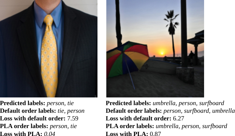
where contains the ground truth label for each time step11 1 Here we consider that is the class-index.. The loss is computed by comparing the prediction of the model at step with the corresponding label at the same step of the ground truth sequence. As can be seen in Equation 3, the order of the ground truth labels is critical to determine the loss a given prediction will receive (see Figure 3). For inherently orderless tasks like multi-label classification, where labels often come in random order, it becomes essential to minimize unnecessary penalization, and several approaches have been proposed in the literature. The most popular solution to improve the alignment between ground truth and predicted labels consists on defining an arbitrary criteria by which the labels will be sorted. Wang et al. wang2016cnn count occurrences of labels in the dataset and sort the labels according to their occurrence in descending order, and is consequently called the frequent-first approach. Jin et al. jin2016annotation use a rare-first approach and dictionary-order in addition to the frequent-first approach. Unlike the frequent-first approach, the rare-first promotes the rare classes in the dataset, while dictionary-order sorts the labels in alphabetical order. The rare-first approach was also adopted by Liu et al. liu2017semantic. Sorting the ground truth labels with a fixed, arbitrary, criteria is shown to improve results with respect to using a random ordering, since the network can learn to predict in the defined order, and avoid part of the loss. However, this will delay convergence, as the network will have to learn the arbitrary ordering in addition to predicting the correct labels given the image. Furthermore, any misalignment between the predictions and the labels will still result in higher loss and misleading updates to the network. Additionally, the frequency of a label in a dataset is independent of the size of the object in a given image. Less frequent but bigger objects can cause the LSTM prediction to stop earlier because of their dominance in the image and their ranking in the prediction step. This issue can be observed in Figure 1, both for the frequent-first and rare-first approaches.
3.3 Orderless recurrent models
To alleviate the problems caused by imposing a fixed order to the labels, we propose to align them to the predictions of the network before computing the loss. We consider two different strategies to achieve this.
The first strategy, called minimal loss alignment (MLA) is computed with:
| (4) | ||||||
where is a permutation matrix, which is constrained to have a ground truth label for each time step: , and that each label in the ground truth should be assigned to a time step. The matrix is chosen in such a way as to minimize the summed cross entropy loss. This minimization problem is an assignment problem and can be solved with the Hungarian kuhn1955hungarian algorithm.
We also consider the predicted label alignment (PLA) solution. If we predict a label which is in the set of ground truth labels for the image, then we do not wish to change it. That leads to the following optimization problem:
| (5) | ||||||
where is the label predicted by the model at step . Here we first fix those elements in the matrix for which we know that the prediction is in the ground truth set , and apply the Hungarian algorithm to assign the remaining labels (with same constraints as Eq. 4). This second approach results in higher losses than the first one (Eq. 4), since there are more restrictions on matrix . Nevertheless, this method is more consistent with the labels which were actually predicted by the LSTM.
To further illustrate our proposed approach to train orderless recurrent models we consider an example image and its cost matrix (see Figure 4). The cost matrix shows the cost of assigning each label to the different time steps. The cost is computed as the negative logarithm of the probability at the corresponding time step. Although the MLA approach achieves the order that yields the lowest loss, in some cases this can cause misguided gradients as it does in the example in the figure. The MLA approach puts the label chair in the time step , although the network already predicts it in the time step . Therefore, the gradients force the network to output chair instead of sports ball although sports ball is also one of the labels.

Orderless training of recurrent models has been previously addressed in vinyals2015order; chen2018order. Vinyals et al. vinyals2015order study the usage of recurrent models to represent sets for which no apparent order of the elements exists. Their method considers two phases: first a uniform prior over all orders is assumed for an initial number of iterations of training, after which in the second phase ancestral sampling is used to sample an ordering. Unlike our method, which proposes to adapt the label order according to the predicted order, their method aims to find the optimal order of the labels (without considering the predicted order). Their method has only been evaluated on a toy problem. More related to our work is the research of Chen et al. chen2018order, which applies a recurrent model without imposing any ordering. This is done by estimating all the labels in the image at every step of the recurrent model. They replace the standard cross entropy loss of the LSTM by a binary cross entropy (BCE). A drawback of this approach is that the LSTM will repeat labels already predicted before. Therefore an additional module needs to be introduced which prevents the method from repeating already predicted labels. An additional drawback of this method is that there is no end-token, so a threshold should be learned to stop the sequence.
4 Experiments
4.1 Datasets and setting
We evaluate our models on four datasets: MS-COCO lin2014microsoft, NUS-WIDE nus-wide-civr09, WIDER Attribute li2016human and PA-100K liu2017hydraplus. MS-COCO is used for image segmentation, image captioning, and object detection. It can be also used for multi-label classification since it has labels for 80 objects. It consists of 82,081 training and 40,137 test images. NUS-WIDE consists of 269,648 images with a total number of 5,018 unique labels. However, annotations for 81 labels are more trustworthy and used for evaluation. After removing the images that do not belong to any of the 81 labels, 209,347 images remain. Following johnson2015love; liu2017semantic, we use 150,000 of these images for training, and rest for testing. For a fair comparison, we create 3 different splits and we pick the best scores on each split and average them to get the final scores. WIDER Attribute is a dataset which has 14 human attributes in 13,789 images with 57,524 annotated bounding boxes (28,345 for training and 29,179 for test). PA-100K is built for evaluating a pedestrian attribute recognition task. It consists of 100,000 pedestrian images with 26 attributes. The size of the training, validation and test sets are 80,000, 10,000 and 10,000 respectively.
Evaluation metrics: We use per-class and overall precision, recall and F1 scores. The per-class metric averages precision and recall scores for each class, and the geometric mean of these averaged values gives the per-class F1 score. In the overall metric, precision and recall scores are computed for all images, and the geometric mean of precision and recall gives the overall F1 score. Only for PA-100K dataset, instead of evaluating accuracy of each label independently, we evaluate accuracy of image-wise class predictions to be able to compare the results with other models. Next, we are interested to see if our method actually adapts dynamically the order to the image, or just learns another (more optimal) fixed order of the classes. To this end, we use an order-rigidness measure on the test set. For each pair of classes, two possible orderings exist (e.g. for classes A and B that would be A-B or B-A); to compute the order-rigidness, we add the number of occurrences of the most frequent order for each pair of classes in the same image, and divide it by the total number of co-occurrences of any pair. We remove all but one of every duplicate prediction without penalization. We show order-rigidness and the percentage of images with duplicate predictions in Table 1.
Network training: We implemented the architecture (see Figure 2) using the PyTorch framework paszke2017automatic. For the encoder part and BCE models we use the VGG16 simonyan2014very, ResNet-50 (for PA-100K) and ResNet-101 he2016deep architectures, and the decoder part is an LSTM with a 512 dimensional internal layer. The word embeddings learned during the training have dimension 256, and the attention module, 512. To train the BCE models, the SGD optimizer is used with learning rate and momentum . For the LSTM models the encoder and the decoder are trained with the ADAM optimizer and Stochastic Weight Averaging izmailov2018averaging with a cyclical learning rate scheduler, decreasing from to in 3 iterations. The BCE models are trained for 40 epochs, and if no improvement is observed after 3 epochs, then we multiply the current learning rate by . For the LSTM models, we fine-tune from the best BCE model and train for 30 epochs more. All the BCE models are pretrained on ImageNet russakovsky2015imagenet. Finally, we do not use the beam search algorithm; we just greedily take the maximum predicted output. Random affine transformations and contrast changes are applied as data augmentation22 2 Our code is available at https://github.com/voyazici/orderless-rnn-classification.
| Algorithms | Ratio of duplicates | Order-rigidness |
|---|---|---|
| Random order | 57.86% | 67.00% |
| Freq. first | 23.84% | 100.00% |
| Rare-first | 29.61% | 100.00% |
| Dict. order | 32.90% | 100.00% |
| MLA | 0.10% | 82.87% |
| PLA | 0.04% | 80.25% |
4.2 Comparison ordering approaches and analysis
We first compare our method to other CNN-RNN optimization strategies such as frequent-first and rare-first, and evaluate several properties of the different methods. Next we compare it against the state-of-the-art on the MS-COCO, NUS-WIDE, WIDER Attribute and PA-100K datasets.
Evaluating training strategies First, we compare the different strategies to train CNN-RNN architectures presented in literature: frequent-first wang2016cnn, rare-first jin2016annotation and dictionary-order jin2016annotation.
As can be seen in Figure 5, our proposed strategies MLA and PLA, which dynamically align the ground truth labels with the predicted labels, train faster and obtain a lower overall loss. The rare and frequent-first approaches obtain substantially higher losses. A significant part of the difference between our approaches and these baselines is that they could potentially obtain a non-zero loss on images in which the model perfectly predicts the correct classes but in the wrong order, as can be seen in Figure 3. For these images, the backpropagated gradient will try to force the prediction to be in the predefined order (a wasted effort in terms of improving the accuracy) despite the sub-optimality of such order for the particular image in some cases, like when the object that should be predicted first is much smaller than the other objects (see Figure 1).
Next, we analyze the number of duplicate labels generated by the various learning strategies (see Table 1). To provide a baseline reference, we also include random order in the table, which refers to a setting where during training the order of the ground truth labels is randomly selected for each mini-batch. The results show that our method manages to learn not to repeat labels that have already been predicted for an image. In principle, one might think, this should be easy for an LSTM to learn. However, because of the imposed order for the frequent and rare-first approaches, and the resulting confusing backpropagated gradients, the LSTM does not learn this and produces many duplicates. Note that duplicates are not penalizing the overall accuracy of the system, since we remove them in a post-processing step. We would also like to point out here that Chen et al. chen2018order require an explicit module for the removal of duplicates generated by their approach, while we train a model that does not generate duplicates in the first place.
In Table 1, we show the results for order-rigidness. They show that the methods which impose a fixed order are actually always predicting labels in that order, as indicated by a 100.00% score. Our methods obtain a 80.25% and a 82.87% score, showing that we have no fixed order for the labels and that it is dynamically adjusted to the image.
4.3 Experimental results
| Algorithms | C-P | C-R | C-F1 | O-P | O-R | O-F1 |
|---|---|---|---|---|---|---|
| BCE wang2016cnn | 59.30 | 58.60 | 58.90 | 61.70 | 65.00 | 63.30 |
| BCE | 68.05 | 59.15 | 63.29 | 72.20 | 65.77 | 68.84 |
| Freq. first | 70.27 | 56.49 | 62.63 | 72.15 | 64.53 | 68.13 |
| Rare-first | 65.68 | 61.32 | 63.43 | 70.82 | 64.73 | 67.64 |
| Dict. order | 70.98 | 55.86 | 62.52 | 74.14 | 62.35 | 67.74 |
| MLA | 68.37 | 60.39 | 64.13 | 72.16 | 66.71 | 69.33 |
| PLA | 68.66 | 60.54 | 64.34 | 72.67 | 66.89 | 69.66 |
| PLA (atten.) | 70.18 | 61.96 | 65.81 | 73.75 | 67.74 | 70.62 |
Comparison of different ordering methods The results of different ordering algorithms can be seen in Table 2. All of the models (except BCE), have the attention module described in the previous section, unless stated otherwise. We observed that the BCE models that we train yield much higher results than the ones cited in previous works, which were originally reported by wang2016cnn and Hu_2016_CVPR for the MS-COCO and NUS-WIDE respectively. Although it is not very clear from wang2016cnn, we think that the difference between our model and theirs is that, during the training, they freeze all the layers except the last one, since when we impose the same restriction to our model, we obtain similar results. Instead, when we allow for full training of the image encoder the results improve significantly, as reported in Tables 2. Interestingly, the fully trained BCE models obtain results similar to those of the CNN-RNN models with the same CNN module when they are trained using the rare-first or frequent-first strategies. We would like to indicate that the results reported in Table 2 are lower than the results that are in the other tables, since we do not exploit augmentations, train fewer epochs and use a part of training set as validation to tune the hyperparameters in these experiments.

When we compare the various strategies of alignment, we see that both our methods, MLA and PLA, clearly outperform the other strategies. Among the other approaches frequent-first yields the best result, although rare-first gives better results with the per-class metric since it assigns more weight to the less common classes. The superior performance of PLA with respect to MLA is interesting: we have empirically found that it is better to align with the actual predictions of the network than to align to obtain the minimal loss, as done in MLA. This phenomenon can be observed in Figure 5. Although MLA yields lower losses than PLA in the beginning, PLA’s alignment with actual predictions of the network leads to a final lower loss and better accuracies. We think that so many penalizations of correctly predicted labels (see Figure 4) takes the optimization further away from the global minimum. In fact, the penalization rate during training is as high as 8% for some classes (e.g. baseball bat). For this reason, we select PLA as our default method instead of MLA when we compare our results with the SOTA. Finally, the attention model improves results with a significant gain.
To further investigate the advantages of the LSTM method over BCE, we compare the co-occurrence matrices of the PLA and BCE method with the co-occurrence matrix of the ground truth for the test set. The co-occurrence matrix is computed with , where are the ground truth labels for image , and respectively replacing the ground truth labels by the predicted labels . Next, the co-occurrence matrix of the ground truth is subtracted to that of the predicted labels (the diagonals are ignored, since the co-occurrences of elements with themselves are irrelevant for our analysis). Figure 6 presents the co-occurrence matrices of the BCE and LSTM (PLA) models on the sports supercategory of the MS-COCO dataset. We can observe that BCE has higher co-occurence values, and larger differences with the ground truth. Given that BCE predicts all labels independently from each other, it cannot prevent re-using evidence already used by another prediction. This can be seen, for example, in the many extra co-occurences of predictions for skis and snowboards, as well as for sports ball and frisbee. Similar cases can be observed on the co-occurrence matrices of other supercategories which are available in the supplementary material. Recurrent models, instead, naturally factor in previous predictions at every time step, which leads to a more realistic co-occurrence in the predictions.
| Algorithms | Architectures | C-P | C-R | C-F1 | O-P | O-R | O-F1 |
|---|---|---|---|---|---|---|---|
| CNN-RNN wang2016cnn | VGG16 | 66.00 | 55.60 | 60.40 | 69.20 | 66.40 | 67.80 |
| Chen et al. chen2018order | ResNet152 | 71.60 | 54.80 | 62.10 | 74.20 | 62.20 | 67.70 |
| SR CNN-RNN liu2017semantic | VGG16 | 67.40 | 59.83 | 63.39 | 76.63 | 68.73 | 72.47 |
| Chen et al. chen2018recurrent | VGG16 | 78.80 | 57.20 | 66.20 | 84.00 | 61.60 | 71.10 |
| Li et al. li2018attentive | VGG16 | 71.90 | 59.60 | 65.20 | 74.30 | 69.70 | 71.80 |
| MS-CNN+LQP niu2019multi | ResNet101 | 67.48 | 60.93 | 64.04 | 70.22 | 67.93 | 69.06 |
| LSEP li2017improving | VGG16 | 73.50 | 56.40 | 63.82 | 76.30 | 61.80 | 68.29 |
| MLIC-KD-WSD liu2018mlickdwsd | VGG16 | - | - | 69.20 | - | - | 74.00 |
| SRN zhu2017learning | ResNet101 | 81.60 | 65.40 | 71.20 | 82.70 | 69.90 | 75.80 |
| ACfs guo2019visual | ResNet101 | 77.40 | 68.30 | 72.20 | 79.80 | 73.10 | 76.30 |
| PLA | VGG 16 | 73.72 | 63.18 | 68.05 | 78.25 | 68.76 | 73.20 |
| PLA | ResNet101 | 80.38 | 68.85 | 74.17 | 81.46 | 73.26 | 77.14 |
| PLA | ResNet152 33 3 Input size of (smaller than ResNet101) to compare with chen2018order. | 75.32 | 69.62 | 72.36 | 76.85 | 73.97 | 75.38 |
| Algorithms | C-P | C-R | C-F1 | O-P | O-R | O-F1 |
|---|---|---|---|---|---|---|
| CNN-RNN wang2016cnn | 40.50 | 30.40 | 34.70 | 49.90 | 61.70 | 55.20 |
| Chen et al. chen2018order | 59.40 | 50.70 | 54.70 | 69.00 | 71.40 | 70.20 |
| SR CNN-RNN liu2017semantic | 55.65 | 50.17 | 52.77 | 70.57 | 71.35 | 70.96 |
| Li et al. li2018attentive | 44.20 | 49.30 | 46.60 | 53.90 | 68.70 | 60.40 |
| LSEP li2017improving | 66.70 | 45.90 | 54.38 | 76.80 | 65.70 | 70.82 |
| MLIC-KD-WSD liu2018mlickdwsd | - | - | 58.70 | - | - | 73.70 |
| PLA | 60.67 | 52.40 | 56.23 | 71.96 | 72.79 | 72.37 |
Comparison to state-of-the-art We compare our results with several models, grouped into two categories: models that use a CNN-RNN jointly and models that use alternative approaches. CNN-RNN wang2016cnn, SR CNN-RNN liu2017semantic and Chen et al. chen2018order are directly related to our model (see sec. 2 for details). Also in this category, Chen et al. chen2018recurrent use an LSTM to predict the next region to attend according to the hidden state and the current region, after which they fuse the predictions of each time step. Similarly, Li et al. li2018attentive use a recurrent network to highlight image regions to attend, but then employ reinforcement learning to select which regions should be used for the actual prediction. Among the alternative approaches, MS-CNN+LQP niu2019multi tries to explicitly predict the number of tags in images, LSEP li2017improving uses a pairwise ranking approach for training a CNN, and MLIC-KD-WSD liu2018mlickdwsd use knowledge distillation from a teacher network which is trained on a weakly supervised detection task. ACfs guo2019visual, proposes a two-branch network with an original image and its transformed image as inputs and imposes an additional loss to ensure the consistency between attention heatmaps of both versions. SRN zhu2017learning proposes a Spatial Regularization Network that generates attention maps for all labels and models the label correlations via learnable convolutions. HP-Net liu2017hydraplus proposes a novel attention module to train multi-level and multi-scale attention-strengthened features for pedestrian analysis. The results on the mentioned datasets can be seen in Tables 4, 5, 6 and 7.44 4 Ge et al. ge2018multi also evaluate on COCO, however they require additional semantic maps which makes their model incomparable.
| Algorithms | C-P | C-R | C-F1 | O-P | O-R | O-F1 |
|---|---|---|---|---|---|---|
| SRN zhu2017learning | - | - | 75.90 | - | - | 81.30 |
| ACfs guo2019visual | 81.30 | 74.80 | 77.60 | 84.10 | 80.70 | 82.40 |
| PLA | 81.69 | 75.87 | 78.67 | 84.99 | 81.36 | 83.13 |
| Algorithms | Precision | Recall | F1 | Accuracy |
|---|---|---|---|---|
| DM li2015multi | 82.24 | 80.42 | 81.32 | 70.39 |
| HP-Net liu2017hydraplus | 82.97 | 82.09 | 82.53 | 72.19 |
| ACfs guo2019visual | 88.97 | 86.26 | 87.59 | 79.44 |
| PLA | 88.50 | 86.67 | 87.58 | 79.83 |
On the MS-COCO dataset, we get higher F1 scores than all other CNN-RNN models. MLIC-KD-WSD liu2018mlickdwsd also achieves notable results by exploiting knowledge distillation from a teacher network. Only for MS-COCO, we resize input images to to be able to compare PLA ResNet-101 model with the ACfs guo2019visual. We also show the results for the ResNet-152 architecture to compare with chen2018order.
On the NUS-WIDE dataset, we surpass all other CNN-RNN models by a significant margin. Our results are especially remarkable for per-class F1 score, a more relevant metric for unbalanced datasets such as this. The globally best results are achieved in terms of overall and per-class F1 score by MLIC-KD-WSD liu2018mlickdwsd. All the models that are compared on NUS-WIDE dataset use the VGG16 as the backbone network. We do not display the results of niu2019multi since they use a different split of the dataset.
To be comparable with other models, we use ResNet-101 and ResNet-50 architectures for WIDER Attribute and PA-100K respectively. These two datasets have human attributes that are related to gender, appearance, clothing, etc. as labels. Therefore, label correlations are not common among these two datasets, which is a drawback for CNN-RNN models. In spite of that, our CNN-RNN model manages to surpass the other models.
5 Conclusions
We proposed an approach for training orderless LSTM models applied to multi-label classification task. Previous methods imposed an ordering on the labels to train the LSTM model, Typically frequent-first or rare-first orderings were used. Instead, we proposed two alternative losses which dynamically order the labels based on the prediction of the LSTM model. Our approach is unique in that seldomly generates any duplicate prediction, and that it minimizes the loss faster than the other methods. Results show that a standard CNN-RNN architecture, when combined with our proposed orderless loss, obtains the state-of-the-art results for multi-label classification on several datasets.
Acknowledgements. We thank the Spanish project TIN2016- 79717-R, the Industrial Doctorate Grant 2016 DI 039 of the Ministry of Economy and Knowledge of the Generalitat de Catalunya, and also its CERCA Program.
References
- (1) S. Bai. A survey on automatic image caption generation. Neurocomputing, 311:291 – 304, 2018.
- (2) Liang-Chieh Chen, Alexander Schwing, Alan Yuille, and Raquel Urtasun. Learning deep structured models. In ICML, pages 1785–1794, 2015.
- (3) Shang-Fu Chen, Yi-Chen Chen, Chih-Kuan Yeh, and Yu-Chiang Frank Wang. Order-free rnn with visual attention for multi-label classification. In AAAI Conference on Artificial Intelligence, 2018.
- (4) Tianshui Chen, Zhouxia Wang, Guanbin Li, and Liang Lin. Recurrent attentional reinforcement learning for multi-label image recognition. In Thirty-Second AAAI Conference on Artificial Intelligence, 2018.
- (5) X. Chen and C. Zitnick. Mind’s eye: A recurrent visual representation for image caption generation. In CVPR, 2015.
- (6) Kyunghyun Cho, Bart van Merrienboer, Caglar Gulcehre, Dzmitry Bahdanau, Fethi Bougares, Holger Schwenk, and Yoshua Bengio. Learning phrase representations using rnn encoder-decoder for statistical machine translation. In Learning Phrase Representations using RNN Encoder-Decoder for Statistical Machine Translation, 2014.
- (7) Tat-Seng Chua, Jinhui Tang, Richang Hong, Haojie Li, Zhiping Luo, and Yan-Tao Zheng. Nus-wide: A real-world web image database from national university of singapore. In Proc. of ACM Conf. on Image and Video Retrieval (CIVR’09), Santorini, Greece., July 8-10, 2009.
- (8) J. Donahue, L. Hendricks, S. Guadarrama, M. Rohrbach, S. Venugopalan, . Saenko, and T.Darrell. Long-term recurrent convolutional networks for visual recognition and description. In CVPR, 2015.
- (9) H. Fang, S. Gupta, F. Iandola, R. Srivastava, L. Deng, and P. Dollár others. From captions to visual concepts and back. In CVPR, pages 1473–1482, 2015.
- (10) Weifeng Ge, Sibei Yang, and Yizhou Yu. Multi-evidence filtering and fusion for multi-label classification, object detection and semantic segmentation based on weakly supervised learning. In CVPR, pages 1277–1286, 2018.
- (11) Nadia Ghamrawi and Andrew McCallum. Collective multi-label classification. In Proceedings of the 14th ACM international conference on Information and knowledge management, pages 195–200. ACM, 2005.
- (12) Yunchao Gong, Yangqing Jia, Thomas Leung, Alexander Toshev, and Sergey Ioffe. Deep convolutional ranking for multilabel image annotation. arXiv preprint arXiv:1312.4894, 2013.
- (13) Alex Graves, Navdeep Jaitly, and Abdel-rahman Mohamed. Hybrid speech recognition with deep bidirectional lstm. In IEEE workshop on automatic speech recognition and understanding, pages 273–278, 2013.
- (14) Hao Guo, Kang Zheng, Xiaochuan Fan, Hongkai Yu, and Song Wang. Visual attention consistency under image transforms for multi-label image classification. In CVPR, pages 729–739, 2019.
- (15) Yuhong Guo and Suicheng Gu. Multi-label classification using conditional dependency networks. In Twenty-Second International Joint Conference on Artificial Intelligence, 2011.
- (16) Kaiming He, Xiangyu Zhang, Shaoqing Ren, and Jian Sun. Deep residual learning for image recognition. In CVPR, pages 770–778, 2016.
- (17) Sepp Hochreiter and Jürgen Schmidhuber. Long short-term memory. Neural computation, 9(8):1735–1780, 1997.
- (18) Md. Zakir Hossain, Ferdous Sohel, Mohd Fairuz Shiratuddin, and Hamid Laga. A Comprehensive Survey of Deep Learning for Image Captioning. ACM Computing Surveys, 51(6):1–36, feb 2019.
- (19) Hexiang Hu, Guang-Tong Zhou, Zhiwei Deng, Zicheng Liao, and Greg Mori. Learning structured inference neural networks with label relations. In CVPR, June 2016.
- (20) Pavel Izmailov, Dmitrii Podoprikhin, Timur Garipov, Dmitry Vetrov, and Andrew Gordon Wilson. Averaging weights leads to wider optima and better generalization. arXiv preprint arXiv:1803.05407, 2018.
- (21) Jiren Jin and Hideki Nakayama. Annotation order matters: Recurrent image annotator for arbitrary length image tagging. In Proc. ICPR, pages 2452–2457. IEEE, 2016.
- (22) Justin Johnson, Lamberto Ballan, and Li Fei-Fei. Love thy neighbors: Image annotation by exploiting image metadata. In ICCV, pages 4624–4632, 2015.
- (23) J. Johnson, A. Karpathy, and L. Fei-Fei. Densecap: Fully convolutional localization networks for dense captioning. ICCV, 2015.
- (24) A. Karpathy and L. Fei-Fei. Deep visual-semantic alignments for generating image descriptions. In CVPR, 2015.
- (25) R. Kiros, R. Salakhutdinov, and R. Zemel. Unifying visual-semantic embeddings with multimodal neural language models. TACL, 2015.
- (26) Harold W Kuhn. The hungarian method for the assignment problem. Naval research logistics quarterly, 2(1-2):83–97, 1955.
- (27) Dangwei Li, Xiaotang Chen, and Kaiqi Huang. Multi-attribute learning for pedestrian attribute recognition in surveillance scenarios. In 2015 3rd IAPR Asian Conference on Pattern Recognition (ACPR), pages 111–115. IEEE, 2015.
- (28) Liang Li, Shuhui Wang, Shuqiang Jiang, and Qingming Huang. Attentive recurrent neural network for weak-supervised multi-label image classification. In 2018 ACM Multimedia Conference on Multimedia Conference, pages 1092–1100. ACM, 2018.
- (29) Yining Li, Chen Huang, Chen Change Loy, and Xiaoou Tang. Human attribute recognition by deep hierarchical contexts. In ECCV, pages 684–700. Springer, 2016.
- (30) Yuncheng Li, Yale Song, and Jiebo Luo. Improving pairwise ranking for multi-label image classification. In CVPR, pages 3617–3625, 2017.
- (31) Tsung-Yi Lin, Michael Maire, Serge Belongie, James Hays, Pietro Perona, Deva Ramanan, Piotr Dollár, and C Lawrence Zitnick. Microsoft coco: Common objects in context. In ECCV, pages 740–755. Springer, 2014.
- (32) Feng Liu, Tao Xiang, Timothy M Hospedales, Wankou Yang, and Changyin Sun. Semantic regularisation for recurrent image annotation. In CVPR, pages 2872–2880, 2017.
- (33) Xihui Liu, Haiyu Zhao, Maoqing Tian, Lu Sheng, Jing Shao, Shuai Yi, Junjie Yan, and Xiaogang Wang. Hydraplus-net: Attentive deep features for pedestrian analysis. In ICCV, pages 350–359, 2017.
- (34) Yongcheng Liu, Lu Sheng, Jing Shao, Junjie Yan, Shiming Xiang, and Chunhong Pan. Multi-label image classification via knowledge distillation from weakly-supervised detection. In ACM International Conference on Multimedia, pages 700–708, 2018.
- (35) J. Mao, W. Xu, Y. Yang, J. Wang, Z. Huang, and A. Yuille. Deep captioning with multimodal recurrent neural networks (m-rnn). ICLR, 2015.
- (36) Yulei Niu, Zhiwu Lu, Ji-Rong Wen, Tao Xiang, and Shih-Fu Chang. Multi-modal multi-scale deep learning for large-scale image annotation. IEEE Transactions on Image Processing, 28(4):1720–1731, 2019.
- (37) Adam Paszke, Sam Gross, Soumith Chintala, Gregory Chanan, Edward Yang, Zachary DeVito, Zeming Lin, Alban Desmaison, Luca Antiga, and Adam Lerer. Automatic differentiation in pytorch. In NIPS-W, 2017.
- (38) Luis Pineda, Amaia Salvador, Michal Drozdzal, and Adriana Romero. Elucidating image-to-set prediction: An analysis of models, losses and datasets. arXiv preprint arXiv:1904.05709, 2019.
- (39) Jesse Read, Bernhard Pfahringer, Geoff Holmes, and Eibe Frank. Classifier chains for multi-label classification. Machine learning, 85(3):333, 2011.
- (40) D.E. Rumelhart, G.E. Hintont, and R.J. Williams. Learning representations by back-propagating errors. Nature, 323(6088):533–536, 1986.
- (41) Olga Russakovsky, Jia Deng, Hao Su, Jonathan Krause, Sanjeev Satheesh, Sean Ma, Zhiheng Huang, Andrej Karpathy, Aditya Khosla, Michael Bernstein, et al. Imagenet large scale visual recognition challenge. International journal of computer vision, 115(3):211–252, 2015.
- (42) Karen Simonyan and Andrew Zisserman. Very deep convolutional networks for large-scale image recognition. arXiv preprint arXiv:1409.1556, 2014.
- (43) Nitish Srivastava, Elman Mansimov, and Ruslan Salakhudinov. Unsupervised learning of video representations using lstms. In ICML, pages 843–852, 2015.
- (44) Ilya Sutskever, Oriol Vinyals, and Quoc V Le. Sequence to sequence learning with neural networks. In NIPS, pages 3104–3112, 2014.
- (45) Oriol Vinyals, Samy Bengio, and Manjunath Kudlur. Order matters: Sequence to sequence for sets. In ICLR, 2016.
- (46) Oriol Vinyals, Alexander Toshev, Samy Bengio, and Dumitru Erhan. Show and tell: A neural image caption generator. In CVPR, pages 3156–3164, 2015.
- (47) O. Vinyals, A. Toshev, S. Bengio, and D. Erhan. Show and tell: A neural image caption generator. In CVPR, pages 3156–3164, 2015.
- (48) Jiang Wang, Yi Yang, Junhua Mao, Zhiheng Huang, Chang Huang, and Wei Xu. Cnn-rnn: A unified framework for multi-label image classification. In CVPR, pages 2285–2294, 2016.
- (49) Yunchao Wei, Wei Xia, Junshi Huang, Bingbing Ni, Jian Dong, Yao Zhao, and Shuicheng Yan. Cnn: Single-label to multi-label. arXiv preprint arXiv:1406.5726, 2014.
- (50) Kelvin Xu, Jimmy Ba, Ryan Kiros, Kyunghyun Cho, Aaron Courville, Ruslan Salakhudinov, Rich Zemel, and Yoshua Bengio. Show, attend and tell: Neural image caption generation with visual attention. In International conference on machine learning, pages 2048–2057, 2015.
- (51) K. Xu, J. Ba, R. Kiros, K. Cho, A. Courville, R. Salakhudinov, R. Zemel, and Y. Bengio. Show, attend and tell: Neural image caption generation with visual attention. In ICML, 2015.
- (52) Feng Zhu, Hongsheng Li, Wanli Ouyang, Nenghai Yu, and Xiaogang Wang. Learning spatial regularization with image-level supervisions for multi-label image classification. In CVPR, pages 5513–5522, 2017.
Supplementary Material for Orderless Recurrent Models for Multi-label Classification
1 Introduction
This is the supplementary material of the paper Orderless Recurrent Models for Multi-label Classification. We first exhibit some images whose labels are sorted differently by the proposed predicted label alignment (PLA) and frequent-first approach. Then, we show co-occurrence matrices of different super-categories of the MS-COCO dataset computed by the best BCE and LSTM models.
2 Qualitative comparison of PLA and other methods
In Figures 1-2, we can see different orders yielded by the PLA and frequent-first approaches. The images are chosen to emphasize the problems with the approaches that use predefined orders. As can be seen in the images, the frequent-first approach always predicts the labels in the same order. This leads to confusion in case of dominant but less frequent objects or minor but more frequent objects in an image. Then, this confusion leads to duplicate predictions in different time steps.
3 Additional co-occurrence matrices of LSTM and BCE models
In Figure 3, the predicted class co-occurence matrices for binary cross entropy (BCE) and predicted label alignment (PLA) models can be seen. The levels of co-occurence in BCE are noticeably higher than those on PLA, as it re-uses the same parts of image for different predictions of similar objects (e.g. bike and motorbike). This can be observed especially on the animals, food, vehicle and kitchen super-categories. In the animals super-category the BCE model overshoots co-occurrence of dogs-cats and horses-cows, while in the vehicles the confusion is on the buses, trucks and cars. In the kitchen super-category the confusion is the worst since most of the images are images of entire kitchens and the BCE model uses the entire scene for different predictions. On the other hand, the LSTM model has much lower differences with the ground truth, since the previous predictions are taken into account at every time step.


