Subjective Logic-based Identification of Markov Chains and Its Application to CAV’s Safety∗
Abstract
A reliable estimation of the communication channel which connects automated vehicles is an important step towards the safety of connected and automated vehicles. The communication channel is usually modeled as Markov chain with slowly time-varying transition rates and is identified through statistics on the observed state transitions. However, the classical identification approach lacks a measure on how reliable the identification results, and thus the channel, are. In this work, we propose an identification method, based on the subjective logic theory, which features such a reliability measure in terms of statistical uncertainty. We demonstrate through simulations that the proposed method is capable of quickly responding to parameter changes. Furthermore, it is shown that the transition rates of the Markov chain are tracked with high accuracy. Finally, we validate our results by a real-world experiment.
I INTRODUCTION
Estimating the reliability of cooperative information, which is shared among automated vehicles (AVs), is a big step on the way towards evolving AVs into connected and automated vehicles (CAVs). Reliable cooperative information, arriving with low latency at the CAV, can significantly increase the efficiency and benefit the safety of automated driving [1]. However, if the restrictive requirements of safety critical applications, such as motion planning of a CAV, to the latency are not met, this may result in harm [1].
Identifying the properties of a communication channel to estimate its reliability is a long studied problem dating back to the works of Gilbert [2] and Elliot [3] in the 1960s, which resulted in the Gilbert-Elliot model. Although more sophisticated models exist today, the Gilbert-Elliot model is still frequently used [4]. A channel model as well as the identified parameters thereof are usually used subsequently to estimate the reliability of the communication link [5], e.g., for vehicle-to-anything (V2X) applications [6]. However, existing approaches neglect the statistical uncertainty corresponding to the identified results. We, in turn, argue that these statistical uncertainties can significantly contribute to the reliability estimation and thus should not be neglected.
In this work, we propose a method to identify the communication channel which is modeled as Markov chain and is used for V2X communication based on subjective logic (SL). SL is a mathematical theory that allows to explicitly model the statistical uncertainty of the identified probabilistic model [7]. Thus, in addition to the identified parameters, the reliability of the identification result is estimated. This information, on the one hand, can be used in the CAVs to decide whether a CAV should rely on the cooperative information or fall back to AV mode. On the other hand, we show that the SL result can be used to efficiently recognize and track parameter changes such as jumps or drifts.
The contribution of this paper is twofold: from a theoretical perspective, to the best of our knowledge, there has not yet been developed a method where time-varying Markov chains are integrated into the SL framework. From a practical perspective, we show how the proposed method can be used to estimate the reliability of the V2X communication link of CAVs. If the communication link is not reliable enough, the CAV can terminate the link and is able to fall back to AV mode. Thus, the safety of CAVs is increased.
II RELATED WORK
From a theoretical perspective, to the best of our knowledge, evidence-based subjective logic (EBSL) [8] is the extension of SL most closely related to our proposition. The key idea of EBSL is to combine flow-based reputation systems with the uncertainty concept of SL to determine indirect computational trust through a trust network. Flow-based reputation systems, in turn, have their mathematical foundation in Markov chains. Thus, EBSL indirectly links Markov chains to SL. However, EBSL requires the underlying Markov chain to be static. Furthermore, the underlying Markov chain is constrained by having only two states, as EBSL is only defined for binary opinions (see Section III). In contrast, in this work, we propose an algorithm to identify Markov chains with an arbitrary finite number of states. In addition, the proposed algorithm is able to track the parameters of a time-varying Markov chain.
From a practical perspective, reliability estimation with respect to quality of service (QoS) has to be distinguished from the semantic reliability estimation. For example, in [9], we have proposed such a semantic reliability estimation mechanism and demonstrated its ability through experiment. In contrast, in this work, we focus on the reliability estimation of the QoS. While several works, e.g., [4], [5], [6], have modeled the communication link and thereby achieved good results for highly reliable communication links, however, none of these works considers the statistical uncertainty within the identified model parameters used for the reliability estimation.
III SUBJECTIVE LOGIC BASICS
In this section, we briefly summarize the subjective logic basics used in this paper. The definitions and theorems are based on [7], where further details can be found.
Definition 1 (Subjective Logic Opinion): Let be a random variable of the finite domain with the cardinality . A subjective logic opinion (opinion in short) is an ordered triple with
| (1a) | ||||
| (1b) | ||||
Hereby, is the belief mass distribution over , is the uncertainty mass representing the lack of evidence and is the base rate distribution over representing the prior probability. Moreover, the projected probability
| (2) |
represents the expected outcome of an opinion.
Subjective logic opinions express some information about a random variable in terms of belief, uncertainty, and base rate. One key aspect of opinions is that they are linked to classical probability theory by a bijective mapping to Beta or Dirichlet probability density functions (PDF).
Definition 2 (Dirichlet Distribution): Let be a domain of mutually disjoint values, be the evidence for outcome with , a prior distribution over , and the probability distribution over . Then, the PDF
| (3) |
where and for , is called Dirichlet PDF. A Dirichlet PDF with is called -distribution. In (3), is the well-known Gamma function [10].
Theorem 1 (Equivalent Mapping [7]): Let be a subjective logic opinion and a Dirichlet PDF over the same variable on domain . Then, the equivalent mapping
| (4) |
transforms the Dirichlet distribution into the subjective logic opinion and vice versa.
To combine opinions from various sources, there exists multiple fusion operators to merge these opinions.
Definition 3 (Aleatory Cumulative Belief Fusion): Let and be source A and B’s respective opinions over the same variable on domain . Let be the opinion such that
| (5) |
where and , then the operator in is called aleatory cumulative belief fusion.
To obtain trust or belief from transitive trust paths, trust discounting is often used; for further details refer to [7].
Definition 4 (Trust Discounting): Let be source A’s opinions over the variable on domain . Furthermore, let be the discount probability. Then, the function that yields the opinion such that
| (6) |
holds, is called trust discounting.
IV SUBJECTIVE LOGIC-BASED IDENTIFICATION OF A MARKOV CHAIN
In this section, starting from the problem formulation, an overview of the SL-based identification algorithm is given and the respective steps are explained in detail.
IV-A Problem Formulation
Let be a Markov chain [10] with random variables at time and state space . Then, the transition probabilities are defined as such that the so-called transition matrix is given by . Using , the probability vector can be calculated with
| (7) |
The goal is to identify from realizations. Further, a reliability measure is needed that indicates how certain the identified is based on statistical evidence.
IV-B Algorithm
The key idea of the algorithm is, firstly, to form a rough opinion of the transition matrix based on a buffered sliding window of samples and, consequently, check the opinion for consistency with the previous opinion on that matrix. If the opinions concur, the new opinion will be merged with the previous one, which results in an overall opinion that is based on more statistical data and, thus, features less statistical uncertainty. If, in turn, the opinions do not concur, the previous opinion will be discarded and the new one is chosen. Hence, the algorithm can react quickly to sudden changes such as jumps in the parameters. In contrast, slow changes in the parameters, e.g., drifts, are compensated for, as the new data updates the opinion and the old data is weighted less due to trust discounting. Algorithm 1 gives an overview of one iteration of the algorithm, while the two basic steps, namely the preprocessing and the consistency check, are discussed in detail in the following sections.
IV-C Preprocessing
In order to reach some statistical reliability, samples are buffered in the sliding window where is the window length. The choice of is a trade-off. On the one hand, large values of result in high statistical reliability, thus, the consistency check has to deal with less statistical uncertainty and the system does not immediately react to some statistical variations in the data. On the other hand, small window sizes result in higher dynamics. Hence, the CAV is able to react more quickly to parameter changes.
Then, the statistics are determined on the individual transitions from state to observed in . Based on these statistics, the respective opinions
| (8) |
IV-D Consistency Test
During the preprocessing, the opinion is calculated under the assumption that the actual transition matrix remains constant within the observation window . This assumption, however, is not always true, as the parameters might have changed within with the probability . Even more likely, with the probability , the actual transition matrix might have changed since . This is accounted for by applying trust discounting on both, and .
To check whether or not the transition matrix, estimated in , is still consistent with the previously determined opinion , the opinions are compared with respect to their degree of conflict (DC) [7]. Hereby, the DC is defined as
| (9) |
If the opinions and are similar, the DC is expected to be small, but not zero due to statistical variations. Thus, a threshold is introduced for the . If , the opinions are considered to concur, thus is updated using cumulative belief fusion, i.e., . In contrast, if , the opinions are considered to be inconsistent which indicates that the transition matrix has significantly changed between and . Thus, the previous opinion is discarded and replaced by . Finally, the results are summarized in matrix notation, i.e., and .
V SIMULATIONS
The identification algorithm is exemplarily evaluated through simulations of a communication channel with burst errors. The channel is modeled as Markov chain with two states: good (G) and bad (B). Thus, (7) turns into
| (10) |
Fig. 1 shows the ground truth of an exemplary scenario as well as the result of a classical identification of (10) using data windows of length . For this scenario, a Long Term Evolution (LTE) radio link is assumed to be evaluated for packet loss before the Hybrid Automated Response Request (HARQ) [11]. Typically, to maximize the effective throughput, the radio link is configured such that about of the packets have to be corrected by the HARQ mechanism [11]. As a result, usually, less than of the packets need further corrections. Hence, to simulate a realistic scenario, we start with . The scenario is evaluated over packets, while at packet and sudden changes occur. The jumps take place at prime numbers to avoid an overly quick response due to matching the window size to the jump. In between, the scenario shows a parameter drift. Thus, the algorithm is evaluated for both, namely the adaption to drifts and jumps.
In comparison, Fig. 2 shows the identification result of the proposed SL-based algorithm. It can be seen that the algorithm can track the statistical parameters with higher accuracy while it responds equally quick to the jumps. On top of that, the new algorithm features a measure of the statistical uncertainty which is depicted in Fig. 2(b). The peaks in the uncertainty result from the inconsistency of the opinions at the jumps which is detected by the consistency test.
VI EXPERIMENTS
In our setup, cooperative information from a traffic monitoring system, which observes an occluded intersection, is sent to a Multi-Edge-Computing (MEC) server that computes an environment model from the received data and forwards the model to the CAV via a 5G test mobile network [12]. To merge safely into the occluded intersection, the CAV needs a reliable, low-latency communication link to the MEC server. Thus, the reliability of the communication link must be estimated.
The idea of the presented approach is to infer the reliability of the communication link from the delay times the packets need to travel from the MEC server to the CAV. Therefore, the delays, i.e., the time differences between the timestamps when the MEC server sends a packet and the CAV receives the packet, are monitored.
The test mobile network uses also an HARQ method for error control. Thus, if a packet cannot be decoded immediately, a negative acknowledge (NACK) will be transmitted to request additional redundancy information to decode the packet at the second try [11]. This manifests in an additional delay of about . If the packet cannot be decoded the second time, further delays will occur.
To infer the reliability of the communication link, we first estimate whether a packet has been decoded immediately or had to be reconstructed through HARQ or further error correction mechanisms. We model the communication channel as a three state Markov chain: state 1 denotes that a packet is received correctly, state 2 means that a packet needs HARQ correction which corresponds to slightly distorted conditions, and state 3 implies that a packet needs further correction mechanisms which corresponds to heavily distorted conditions.
Note, however, that the delay of the received packets, even if they are successfully decoded at the first try, depends on multiple factors and thus can slowly vary over time. Therefore, the thresholds, with which the packets are classified as explained above, have to be adapted online. This is done by filtering the recently recorded delays with a moving average filter where outliers are excluded. To achieve a good decision threshold, some additional time is added to the moving average. Fig. 3 shows a sequence of measured packet delays between the MEC server and the CAV as well as the decision borders. It can be seen that most of the packets are within the first region, i.e., below the lower red line, while some are in the second region, i.e., between the red lines, and only very few are in the third region, i.e., above the upper red line.
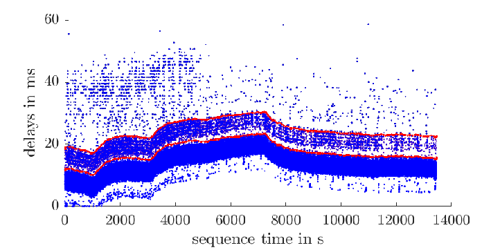
To evaluate these delays quantitatively, delays of about packets were recorded over approximately hours. The sequence is subdivided into subsets of recorded packet delays. The delays within these subsets are classified into immediately decoded, HARQ corrected, and further corrected. The statistics over these subsets are monitored over time. These statistics represent the observed state transition rates of the Markov chain.
Fig. 4 shows the classically estimated state transition rates corresponding to the statistics as well as a smoothed version thereof. It can be seen that the probability of decoding a package at the first try is around at the beginning of the sequence and increases afterwards to . This suits well with the typical radio link configuration. The increase of the decoding probability at the first try can be explained by a heavy rain shower that went over the test mobile network at the beginning of the sequence. The smoothed result of the classical identification is obtained with a moving average filter and is used later as ground truth.
In the next step, the Markov chain is identified using Algorithm 1 on the same data. The identification result is subsequently projected back to the state transition probabilities, as identified with the classical method. Both results are compared in Fig. 5(a), while the statistical uncertainty, which can only be obtained with the new method, is visualized in Fig. 5(b). It shows that the identification result of the proposed online method fits well with the acausally smoothed classical identification, and additionally delivers its uncertainty.
VII CONCLUSIONS
In this work, we proposed a SL-based method to identify Markov chains that integrates Markov chains into the theory of SL. The method has been applied to the reliability estimation of communication channels from CAVs. As reliable communication links are essential for the safety of CAVs, the proposed method is able to increase CAVs’ safety. The method was evaluated through simulated data and validated by a real-world experiment showing that the method is able to track parameter changes in the communication channel. In further work, the method will be tested on other network topologies.
ACKNOWLEDGMENT
We thank Soheil Gherekhloo for the fruitful discussions that helped us to review and improve our work.
References
- [1] J. E. Siegel, D. C. Erb, and S. E. Sarma, “A survey of the connected vehicle landscape—architectures, enabling technologies, applications, and development areas,” IEEE Transactions on Intelligent Transportation Systems, vol. 19, no. 8, pp. 2391–2406, 2018.
- [2] E. N. Gilbert, “Capacity of a burst-noise channel,” The Bell System Technical Journal, vol. 39, no. 5, pp. 1253–1265, 1960.
- [3] E. O. Elliott, “Estimates of error rates for codes on burst-noise channels,” The Bell System Technical Journal, vol. 42, no. 5, pp. 1977–1997, 1963.
- [4] A. Iacovazzi, D. Frassinelli, and Y. Elovici, “On packet loss modeling: An empirical assessment,” in 2017 8th International Conference on the Network of the Future, 2017, pp. 33–39.
- [5] J. Chakravorty and A. Mahajan, “Structure of optimal strategies for remote estimation over gilbert-elliott channel with feedback,” in 2017 IEEE International Symposium on Information Theory, 2017, pp. 1272–1276.
- [6] J. Zhou, D. Tian, Y. Wang, Z. Sheng, X. Duan, and V. C. M. Leung, “Reliability-optimal cooperative communication and computing in connected vehicle systems,” IEEE Transactions on Mobile Computing, 2019.
- [7] A. Jøsang, Subjective Logic. Springer International Publishing, 2016.
- [8] B. Škorić, S. J. de Hoogh, and N. Zannone, “Flow-based reputation with uncertainty: evidence-based subjective logic,” International Journal of Information Security, vol. 15, no. 4, pp. 381–402, 2016.
- [9] J. Müller, M. Gabb, and M. Buchholz, “A subjective-logic-based reliability estimation mechanism for cooperative information with application to iv’s safety,” arXiv preprint arXiv:1903.01556, 2019.
- [10] I. Bronshtein, K. Semendyayev, G. Musiol, and H. Mühlig, Handbook of Mathematics. Springer, Berlin, 2007.
- [11] M. Sauter, From GSM to LTE-advanced: an introduction to mobile networks and mobile broadband. John Wiley & Sons, 2014.
- [12] M. Buchholz, M. Herrmann, J. C. Müller, V. Belagiannis, P. Pavlov, B. Hätty, S. Schulz, and R. W. Henn, “A digital mirror: A mobile edge computing service based on infrastructure sensors,” in 25th Intelligent Transport Systems World Congress, 2018.