Existence of nodal line semi-metal in a generalized three dimensional Haldane model
Abstract
We construct and study a time reversal broken tight binding model on diamond lattice with complex next-nearest-neighbour hopping which can be thought of as a generalisation of two dimensional Haldane model in three dimension. The model also breaks inversion symmetry owing to sub-lattice dependent chemical potential. We calculate the spectrum of the model and find the existence of six pairs of anisotropic gapless points with linear dependence on momentum. The coordinates of the gapless points are ( and their possible permutations . The condition for gapless spectrum is very similar to the two dimensional case. Each gapless points are having well defined chirality and in the gapless phase specific set of planes have non-zero Chern number. The gapped phase is a trivial bulk insulator which has vanishing Chern number as well as Hopf index. The model belongs to the symmetry class AIII according to the ten-fold way of classification. Surprisingly the gapless phase does contain a gapped surface state where as the gapped state has a gapless surface states as found in (1,1,1) direction.
Keywords:
3-d topological insulator; hopf invariant, Pontryjagen invariant, hopf insulatorpacs
Insert PACS number hereI Introduction
Understanding and classification of materials in the group of metal and insulator has been a long time interest
to the scientific endeavour. Starting from the simple prediction of Bloch theorem, we have come across a long
way examining the role of electron-electron interaction, disorder, impurity, pressure, spin-orbit coupling, temperature
etc. In this context, a very intimate and interesting connection of topology with the conductivity tensor has been
established in early 80’s for the integer quantum hall effect(IQHE)thouless-1982. It has been shown that conductivity
tensor is related to Chern number for the problem of electron gas in the presence of magnetic field which breaks the time
reversal symmetry explicitly. Few year later, Haldane showed that external magnetic field is not necessary
condition to have quantized Hall conductivity though time reversal breaking is a necessary ingredient haldane-1988.
A fundamental jump in this direction happened when Kene and Mele showed that time reversal symmetry breaking is not a necessary
ingredient to have a topological insulating phase kane-2005-2nd. The model includes a next-nearest neighbour
spin-orbit coupled hopping on honeycomb lattice. It has been shown that a non-zero quantum spin hall current can be
linked to the same Chern number. However very soon it has been realized that this simple classification on the basis of
Chern number is insufficient for the case of time reversal invariant system. For invariant system, a Z2 classification
has been proposed as the simple Chern number must reduce to zero for non-conserving terms are included in the form of Rashbha
coupling kane-2005-1st.
Very soon the proposed classification was extended to 3 Dimensional time reversal invariant quantum spin hall insulator(QSHI) fu-kane-2007; moore-2007 in terms
of four invariants resulting 16 classes topological insulators. A connection of invariants with the Chern invariants was also shown rahul-2009-1; rahul-2009-2 for the time reversal symmetric(TRS) system. On the other hand in 3 Dimension for time reversal and inversion symmetry broken system halperin-1987; kohmoto-1992; ezzine-2004; guo-2015
has yielded the Weyl systems with non-trivial connection to surface states to bulk gapless mode armitage-2018; murakami-2007; wan-2011; hosur-2012 . These Weyl fermionic systems are natural generalizations relativistic Dirac fermions in 3 Dimensions and topological invariants are the Chirality
which is determined by calculating the Chern number around the gapless Dirac node over a closed surface. However all these models have a four component
structure in momentum space. For two component Hamiltonian in 3 dimension it is realized that a different kind of Topological insulator named
Hopf Insulator exist which is characterized by Hopf invariants which is particularly useful when the other topological invariant named so far
is not directly usable in particular when the Chern number becomes zero in 3 Dimension moore-2008; deng-2013. These motivates us to extend the Haldane model in three dimension in the Diamond lattice which contains next-nearest complex hopping as chosen
in Haldane model. The model involves a spinless fermion hopping in diamond lattice and hamiltonian has only structure for each momentum due to two sub-lattice structure of diamond lattice. Thus it fills an important chapter in the study of three dimensional topological system owing to its absence of both time reversal and inversion symmetry and an effective structure.
The paper has been organized in the following manner. In Sec. II we define the model and its band structure and low energy expansion in momentum space. In Sec. III we discuss the symmetry of the model according to the ten-fold way classification altland-1997; zimbauer-1996; andreas-2008. In Sec. IV numerical calculation of surface state is discussed. In Sec. V we discuss the topology of the model by determining the Chern number and Hopf invariant and discuss its connection with Weyl physics. Finally we conclude our study in sec. VI.
II Extension of Haldane model to 3-dimension
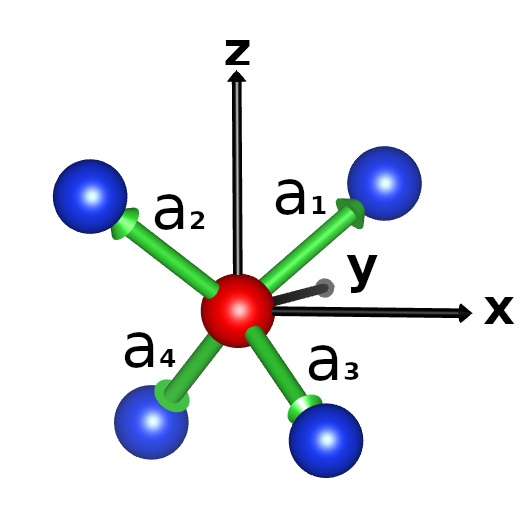
We have chosen the diamond lattice for the extension of Haldane model in 3 dimension for its similarity with two dimensional honeycomb lattice in having hexagonal plaquette as an elementary unit. Diamond lattice has two inter-penetrating FCC sub-lattice denoted by ‘A’ and ‘B’ as shown in the Fig. 1. The Model Hamiltonian we are interested in this study is following,
| (1) | |||||
In the above denotes nearest neighbour (NN) hopping and denotes next nearest neighbour (NNN) hopping between the same sub-lattice. We have taken into account a complex phase with in Haldane sense which breaks the time reversal symmetry explicitly. Here has following properties, , . Details of NN and NNN-vectors are given in the Appendix VII.1. After Fourier transformation in pseudo-spin space Hamiltonian is given by
| (2) |
where is a matrix and is given by,
| (3) | |||||
The various components that appear in are given below with the convention ,
| (4) | |||
| (5) | |||
| (6) | |||
| (7) | |||
| (8) | |||
| (9) |

The dispersion obtained after diagonalization is given below,
| (10) |
From this dispersion relation (Eq- 10) gap closing condition are obtained as follows,
| (11) |
From Eq- 5 and Eq- 9 first condition translates into
| (12) |


Now the condition enforces the gapless points to reside on the nodal line having equation . We have six such nodal lines as presented in Fig. 2. For simplicity, we consider the gap closing point on the nodal line having and yielding and from Eq- 12 we obtain the following condition for gaplessness,
| (13) |
Similar condition for gaplessness can be obtained by replacing to . The above condition for gaplessness can be compared with two dimensional case where one finds . From the Eq. 13, it is clear that for a given and we can find from Eq- 13 at which gap closes. In Fig. 4, we present the regions where the gap closes or not in plane. The region-I denotes the gapless phase and region-II denotes the gapped phase. We notice that gapless points occurs at the isolated points on the nodal line only as shown in Fig. 2. Now it is customary to obtain the low energy effective Hamiltonian around these gapless points. A straightforward calculation starting from Eq- 3 around the nodal line and for any satisfying Eq. 13, we obtain the effective Hamiltonian as,
| (14) |

The various component appearing in the above expressions are as follows,
| (15) | |||
| (16) |
In the above is the values of for which gapless condition is satisfied according to Eq. 13.
From Eq. 14, Eq. 15 and Eq. 16, it is clear that this is an asymmetric Weyl like points. The x-component does depend on the y-component and the z-component is linear combination of more than one component. The label denotes the points at which the above low energy expansion has been obtained. We notice that there are such points and similar expansion can be obtained around each Wyel point.
Generically each such gapless points are characterized by their Chirality and it is given by armitage-2018 where and h is given in Eq. 14, Eq. 15 and Eq. 16. For example, Chirality of gapless point at is . The Chirality of each gapless points which has also been depicted in Fig. 2.
III Symmetry
Following Altland and Zirnbaueraltland-1997, Hamiltonian of non-interacting fermionic systems can be classified on the basis of three basic discrete symmetries such as Time-reversal symmetry (anti-unitary and commutes with the Hamiltonian), Particle-hole symmetry (anti-unitary and anti-commutes with the Hamiltonian) and chirality symmetry (unitary and anti-commutes with the Hamiltonian). In our study we implement the symmetry by the transformation and the inversion symmetry , to the Hamiltonian in Eq- 1. For clarity we denote as the nearest neighbour hopping part of the Eq. 1. Similarly and denote the next-nearest neighbour hopping interaction and denotes the sub-lattice dependent chemical potential term. These various parts of the Hamiltonian undergo the following transformation under followed by .
| (17) | |||
| (18) | |||
| (19) | |||
| (20) |
The above mapping indeed tells that Hamiltonian in Eq. 1 gets an overall negative sign. This symmetry is unitary and anti-commutes with the Hamiltonian and according to ten-fold way of classification it falls in the AIII Chiral classes and this class is characterized by the , infinite cyclic group which must be characterized by some integers.
IV Surface state
Having discussed the spectrum of the model in details, the existence of the asymmetric Weyl like points along the nodal line and necessary symmetry classification, we discuss the nature of surface states. To this end, we calculate the surface state numerically of our model for a slab geometry with the boundary surface in (111) direction, as shown in the Fig. 5. We have found that the gapless phase where the bulk is gapless do contain a gapped surface states as shown in left panel of Fig. 6. In the right panel of Fig. 6, we show the band structure for the same open geometry in gapped phase and find the existence of a pair of gapless surface states that crosses each other twice. In the Fig. 6, we have plotted the band structure in two dimensional- Brillioune zone along a certain direction which deviates from the high symmetry points.


This has been done to include the gapless points along the contour which does not lie on the contour connecting the high symmetry points in the present model. The gapless surface state that exist in the gapped region can be made gapped by changing the parameter values. One easy way to do this is to change the ratio of interlayer and intra layer hopping amplitude. Let and denotes the interlayer and intra layer nearest-neighbour hopping. Similarly and denotes the interlayer and intra layer hopping amplitude. For certain combinations of and , the gap can be opened for the surface state in gapped region. In Fig. 7 we have shown a gapped surface state in gapped region which happens for . Such transition from gapless surface state to gapped surface state can experimentally detected by surface conductance. In Fig. 8 we show absolute value of component of eigenvectors as a heat-map showing how the surface-state appears and decays into bulk starting from one of the open surface. In drawing this figure we have used a projection of one Weyl like points on the two dimensional brillouin zone in the gapless phase. For the gapped phase ‘’ is the point ‘B’ in the right panel of Fig. 6 which is one of the gap closing point for the surface state. In conclusion we have found always a gapped surface state in Region I and gap-less surface state in Region II which can be made gapped by changing the parameter values.


V Chern number and Hopf invariant
Unlike two dimensional topological insulators, the topological classification of three Dimensional systems are more involved. For the time reversal invariant system generally index is used to classify the topology where as for time reversal broken system Chern number can still be used. In the absence of finite Chern no, it has been proposed that Hopf index could be finite and can be used to characterize the system. Though we are dealing with a three dimensional system, substantial amount of information can be extracted from the topological property of two dimensional sub-system which constitute the whole system rahul-2009-1; rahul-2009-2; rahul-2007. Though the connection of Chern number for three dimensional system has been discussed in the context of time reversal invariant system we deduce those for our case as first hand probe to the nature of topology of our system. We note that for the original Haldane model time reversal is broken though there were no external magnetic field was present and it is the Chern number which decided the topological nature of the phases. This also motivates us to derive the Chern number for our system. Since all three directions , and are equivalent, we analyse only for direction and same conclusion holds for all other directions. Let’s consider a set of planes perpendicular to the axis which is intercepted by two nodal lines and . In Fig. 2, the square blue shaded region denotes one such plane. To calculate Chern number for such planes we consider three cases i) . We are going to consider the third case first. Depending on the choice of parameters if changes sign in the plane we can not have single gauge choice throughout and the Berry vector potential in these two region is connected by the relation where is obtained as,
| (21) | |||||
In the above, we have used , , following Eq. 15 and Eq. 16 with . Using short notation as , , and , and . From the above equation, one can show that . Now, since , Chern number for this case is,
| (22) |
Similarly for the first case, , this plane has two consecutive sides along which gap closes. On this plane we have, . So the phase difference is given by, . Hence the Chern no can be found as ,
| (23) |
The above results can be reconciled from the condition in Eq. 13 that for , the gapless condition reduces to and
independent. The above discussion can be summarized in the following way. For the gapless phase as denoted by region-I in Fig. 8, for every plane parallel to plane and having a definite in between the two Weyl-like points, there is a non-zero Chern number for a given . Thus we have found continuous set of parallel plane for which Chern number is non-zero. The above arguments is true for other planes parallel to and plane. In the gapped phase there is no plane having non-zero Chern no. This construction is very similar found earlier rahul-2009-1; rahul-2009-2.
From the analysis of our model Hamiltonian, we have found that the gapless surface state exist for the region where bulk is gapped. On the contrary, the region where bulk is gapless we have gapped surface state. We have also shown in the preceding discussion that there are six planes for which non-zero chern number exist. The gapless phase contains anisotropic Weyl-like points and it is known that generally in such case, there exist a gapless surface states for open systems kundu; sumathi-rev. However our results is in contrast to the existing literature. To explore more on the topology theory we note that it has been established from the homotopy theory that for Hamiltonian having structure in 3 dimension and in the absence of finite Chern number, the Hopf invariant can take finite integer and this signifies a non-trivial topology in 3 dimension moore-2008; deng-2013. It may be noted that for 2 dimension a Hamiltonian in momentum space is a map from . However in 3 dimension a Hamiltonian is a map from . The Hopf invariant is associated with the possible non-triviality of the map . If the Chern numbers in all three directions, the Hopf index takes all integers values and has a simple integral expression
| (24) |
where A is the Berry connection which satisfies and u denotes the map from which in our case is the wave function. The Hopf index is gauge invariant although its expression depends on A. The Hopf invariant is similar to the invariant or Chern parity in topological insulators in that its standard integral expression uses the gauge-dependent quantity A even though the final result is gauge-invariant when the Chern numbers are zero. In our gapped regime where a non-trivial topological surface state exist and the Chern number is zero, we have evaluated numerically the l.h.s of Eq. 24 and found to be zero. Thus unlike the other topological systems moore-2008; deng-2013 which have Chern number zero but finite Hopf index, the gapped phase we find here seems to be trivial bulk insulator.
VI Conclusion
In essence we have studied an extension of two dimension Haldane model haldane-1988 in diamond lattice providing a 3 dimensional generalisation. Both time reversal and inversion symmetry has been broken with complex coupling constant and sub-lattice depended mass term respectively, but keeping chiral symmetry intact. Topological classification has been performed on the basis of dispersion relation, Chern number of two-dimensional sub-systems and existence of surface state in the parameter space has been done. In some region of space the system is gapless only at certain number of k points and we find existence of gapless surface state at k where system is gapped. In the gapless phase there exist 6 pairs asymmetric Weyl-like points with well defined chirality. In the gapless state the surface state is always gapped but in the gapped phase the surface state is gapless or gapped depending on the parameter values. We have calculated Hopf index to characterize this gapped phase but that turnes out to be zero. The insulating phase thus seems to be a trivial bulk insulator.
Acknowledgement
The authors acknowledg many fruitful discussion with Arijit Saha and Kush Saha.
References
- (1) D. J. Thouless, M. Kohomoto, M. P. Nightingale, and M. den Nijs, Phys. Rev. Lett. 49, 405(1982).
- (2) F. D. M. Haldane, Phys. Rev. Lett. 61, 2015(1988).
- (3) C. L. Kane and E. J. Mele, Phys. Rev. Lett. 95, 146802 (2005).
- (4) C. L. Kane and E. J. Mele, Phys. Rev. Lett. 95, 226801 (2005).
- (5) Liang Fu, C. L. Kane, and E. J. Mele, Phys. Rev. Lett. 98, 106803 (2007).
- (6) J. E. Moore and L. Balents, Phys. rev. B 75, 121306(R) (2007).
- (7) Rahul Roy, Phys. Rev. B 79, 19531 (2009).
- (8) Rahul Roy, Phys. Rev. B 79, 19532 (2009).
- (9) B. I. Halperin, Jpn. J. Appl. Phys., Suppl. 26, 1913 (1987).
- (10) M. Kohmoto, B. I. Halperin, and Y. S. Wu, Phys. Rev. B 45, 13488 (1992)
- (11) A.-Z. Ezzine de Blas and F. Axel, J. Phys.: Condens. Matter 16,7673 (2004).
- (12) Xiaoyong Guo, Zaijun Wang, Qiang Zhengand Jie Peng, International Journal of Modern Physics B Vol. 29, No. 6 (2015) 1550034
- (13) N. P. Armitage, E. J. Mele, and Ashvin Vishwanath, Rev. Mod. Phys., Vol. 90, No. 1.
- (14) S. Murakami, New J. Phys. 9, 356 (2007).
- (15) X. Wan, A. M. Turner, A. Vishwanath and S. Y. Savrasov, Phys. Rev. B 83, 205101 (2011)
- (16) P. Hosur, S. A. Parameswaran and A. Vishwanath, Phys. Rev. Lett. 108, 046602 (2012).
- (17) Joel E. Moore, Ying Ran and Xiao-Gang Wen, Phys. Rev. Lett 101, 186805(2008).
- (18) Deng, D.-L. and Wang, S.-T. and Shen, C. and Duan, L.-M., Phys. Rev. B 88, 201105(R).
- (19) A. Altland, M. Zirnbauer, Phys. Rev. B 55, 1142 (1997).
- (20) M. Zimbauer, J. Math. Phys. 37, 4986 (1996).
- (21) Andreas P. Schnyder, Shinsei Ryu, Akira Furusaki and Andreas W. W. Ludwig, Phys. Rev. B 78, 195125(2008)
- (22) Rahul Roy, 2010 New J. Phys. 12 065009.
- (23) U. Khanna, A. Kundu, S. Pradhan and S. Rao, Phys. Rev. B 90, 195430 (2014)
- (24) Sumathi Rao, arXiv:1603.02821
- (25) T. Pereg-Barnea and H.-H. Lin 2005 EPL 69 791.
- (26) Jhih-Shih You, Wen-Min Huang, and Hsiu-Hau Lin, Phys. Rev. B 78. 16140(R)(2008).
- (27) Wen-Min Huang, Toshiya Hikihara, Yen-Chen Lee and Hsiu-Hau Lin, Scientific Report, 7:43678 | DOI: 10.1038/srep43678(2017)
- (28) generatingfunctionology, Herbert S. Wilf, Third Edition,Academic Press(2014)
VII Appendix-A
VII.1 Details co-ordinate system used
Here we first enlist the nearest-neighbour vectors used.
| (25) |
The details of next-nearest-neighbour vectors are given below.
| (26) |
VII.2 surface state
In Sec. IV, we have presented the numerical results for the surface state where the system has been kept open in (1,1,1) direction as shown in Fig. 5. Here we give detail derivation of the equations for such geometry and derive the equations which needs to be solved to obtain the surface states analytically pereg-2005; you-2008; huang-2017 . Following reference wilf, we can easily derive the Harper equation for this slab geometry by defining a Fourier transformation in a two dimension plane equivalent to a honeycomb lattice. The coupled equation that one obtains are given below where and represent that annihilation operator at ‘A’ and ‘B’ sub-lattice and and refers to momentum and layer index respectively.
| (27) |
| (28) |
where , and and , , are shown in the figure 5. The above set of coupled linear homogeneous recursion relation can be solved by method of generating function> For this purpose we define two functions and in the following way
where , are solution of the recursion relations 27, 28 and explicite dependence on ‘’ has been omitted for simplicity. The formal solution for the coefficient and are obtained as,
| (29) | ||||
| (30) |
and , turns out to be
| (31) | ||||
| (32) |
where
| (33) | |||||
| (34) | |||||
| (35) |
In the above, , and denotes complex conjugation. The boundary condition we have used is , and . But this does not affects later analysis since it appears only in the numerator. The above set of equation as given in Eq. 31 and Eq. 32 can be solved using the method of residue. However it turns out that it is not very straightforward to obtain the solution and it will be presented elsewhere