跳到论文正文
W Papers独立论文阅读器 arXiv:1911.09580 论文正文 计算阅读时间 · 0%
引用这篇论文根据当前论文元数据生成,正式投稿前建议核对。


License: arXiv.org perpetual non-exclusive license
arXiv:1911.09580v1 [math.PR] 21 Nov 2019

Distributional Robustness and Uncertainty Quantification for Rare Events

Jeremiah Birrell Email: birrell@math.umass.edu Address: Department of Mathematics and Statistics, University of Massachusetts Amherst, Amherst, MA 01003, USA    Paul Dupuis Email: dupuis@dam.brown.edu Address: Division of Applied Mathematics, Brown University, Providence, RI 02912, USA    Markos A. Katsoulakis Email: markos@math.umass.edu Address: Department of Mathematics and Statistics, University of Massachusetts Amherst, Amherst, MA 01003, USA    Luc Rey-Bellet Email: luc@math.umass.edu Address: Department of Mathematics and Statistics, University of Massachusetts Amherst, Amherst, MA 01003, USA    Jie Wang Email: wang@math.umass.edu Address: Department of Mathematics and Statistics, University of Massachusetts Amherst, Amherst, MA 01003, USA
August 11, 2026
Abstract

Rare events, and more general risk-sensitive quantities-of-interest (QoIs), are significantly impacted by uncertainty in the tail behavior of a distribution. Uncertainty in the tail can take many different forms, each of which leads to a particular ambiguity set of alternative models. Distributional robustness bounds over such an ambiguity set constitute a stress-test of the model. In this paper we develop a method, utilizing Rényi-divergences, of constructing the ambiguity set that captures a user-specified form of tail-perturbation. We then obtain distributional robustness bounds (performance guarantees) for risk-sensitive QoIs over these ambiguity sets, using the known connection between Rényi-divergences and robustness for risk-sensitive QoIs. We also expand on this connection in several ways, including a generalization of the Donsker-Varadhan variational formula to Rényi divergences, and various tightness results. These ideas are illustrated through applications to uncertainty quantification in a model of lithium-ion battery failure, robustness of large deviations rate functions, and risk-sensitive distributionally robust optimization for option pricing.

Keywords: 
distributional robustness, rare events, Rényi divergence, risk-sensitive functional, uncertainty quantification, large deviations
2010 MSC
62B10, 94A17, 60F10, 60E15

1 Introduction

Risk-sensitive quantities-of-interest (QoI), such as rare-events, partition functions, moment generating functions, and exit times, are of great interest in many applications from engineering, biology, chemistry, and finance. Significant model uncertainty stemming from uncertain parameter values, uncertain model form, or some approximation procedure (variational inference, dimension reduction, neglecting memory terms, linearization, asymptotic approximation, etc.), is inherent in many such systems. Therefore, it is important to study the dependence of risk-sensitive QoIs on model perturbations. In [1, 2], it was shown how robustness bounds for risk-sensitive QoIs can be obtained from variational principles involving information-divergences (specifically, Rényi-divergences). Such bounds can be viewed as performance guarantees or stress tests over a collection of alternative models, called an ambiguity set. In this work, we characterize the structure of Rényi-divergence-based ambiguity sets by utilizing the connection between Rényi-divergences and the moment-generating-function (MGF) of the log-likelihood. More specifically, we show how to construct ambiguity sets that correspond to various tail-behavior (stress-test) scenarios. We also extend some of the foundational theory connecting risk-sensitive QoIs to information divergences and robust optimization, including a generalization of the Donsker-Varadhan variational formula to Rényi divergences (see Theorem 5.4). We show how these tools can be combined to obtain explicit uncertainty quantification (UQ) bounds, and illustrate this through several applications: robustness of a data-driven model of lithium-ion battery failure, large deviations rate functions, and robust option pricing.

1.1 Risk-Sensitive QoIs, Ambiguity Sets, and Robust UQ

Refer to caption
Figure 1: Histogram of the battery failure data from [3]. The small number of samples in the tails of the distribution highlights the need for robust UQ when dealing with rare-events and other risk-sensitive QoIs.

As motivation for the notion of ambiguity set and the problem of distributionally robust UQ, consider the data set of 124 lithium-ion-battery failure times from [3]. A typical workflow for analyzing QoIs (expectations of random variables) might consist of:

Data→fit/learn Model, P→QoI τEP​[τ],\displaystyle\text{Data}\xrightarrow[\text{fit/learn}]{}\text{ Model, $P$}\xrightarrow[\text{QoI $\tau$}]{}E_{P}[\tau], (1)

i.e., the baseline model PP (a probability measure) is constructed from the data, and properties of QoIs are computed from PP (EPE_{P} denotes the expectation under PP).

A histogram of the data from [3], shown in Figure 1, illustrates a pervasive, unsurprising, but crucial problem with the process (1) when τ\tau is sensitive to the tail(s) of the distribution, i.e., when τ\tau is risk-sensitive: there is very little data regarding the tails of the distribution! This paucity of data calls into question the computed quantity EP​[τ]E_{P}[\tau] for risk-sensitive τ\tau, e.g., early failure probabilities or the failure rate. This motivates our consideration of the following distributionally robust UQ problem:

𝐁𝐨𝐮𝐧𝐝:log(EQ[τ]),Q∈𝒰.{\bf Bound:}\,\,\,\,\,\,\,\log(E_{Q}[\tau]),\,\,\,Q\in\mathcal{U}. (2)

The robust UQ problem (2) involves bounding the QoI over an ambiguity set, 𝒰\mathcal{U}, of alternative models QQ (probability measures) that are ‘near’ to PP in some sense.

Remark 1.1.

One could equivalently formulate (2) without the logarithm, but in our approach it is generally convenient to include it. This is further motivated by the following: if τ=1A\tau=1_{A} for some (rare) event AA, then the QoI becomes log⁡(P⁡(A))\log(P(A)). In this form, the connection with tail-behavior is apparent, as log⁡(P⁡(A))\log(P(A)) is of central importance in large deviations theory. Our new results, and those of [1, 2], have many connections to large deviations (see also Section 7.2 below), though we are largely interested in obtaining non-asymptotic robustness bounds.

The choice of 𝒰\mathcal{U} in (2) is a modeling choice, and each such ambiguity set can be viewed as a stress-test of EP​[τ]E_{P}[\tau] under tail-perturbations of PP of a particular type. This motivates the stress-test design problem: how does one construct a 𝒰\mathcal{U} that realizes the desired stress test? A solution to this problem is given in Section 3, where we derive a general method for constructing ambiguity sets that correspond to stress-testing EP​[τ]E_{P}[\tau] under a prescribed type of tail-perturbation (i.e., prescribing P⁡(d​Q/d​P≥r)P(dQ/dP\geq r)). For example, 𝒰\mathcal{U} could consist of QQ’s whose tails with respect to PP have power-law decay under PP. A given modeling scenario might motivate a particularly appropriate choice of 𝒰\mathcal{U}; we will discuss this in the examples in Section 7. The neighborhoods we construct will be defined in terms of Rényi-divergences, and are thus capable of capturing non-parametric model perturbations. We also describe several methods of constructing new members of a given ambiguity set, either out of PP or of other known members; these further highlight the non-parametric nature of the results.

Remark 1.2.

The ambiguity set 𝒰\mathcal{U} could be chosen to be a subset of some finite-dimensional parametric family that includes PP (i.e., perturbing the parameters that define PP), and our methods can be applied to such cases. However, our goal here is the development of methods that apply equally well to non-parametric (infinite dimensional) model neighborhoods.

Once an ambiguity set is chosen, the distributional robustness problem of Eq. (2) can be addressed using tools from information theory. Specifically, the following risk-sensitive robustness bounds were proven in [1] (where a similar lower bound can also be found):

Proposition 1.3.

Let P,QP,Q be probability measures on (Ω,ℳ)(\Omega,\mathcal{M}) and g:Ω→ℝg:\Omega\to\mathbb{R} be measurable. Then

log[∫egdQ]≤infc>1{1clog[∫ec​gdP]+1c−1Rc/(c−1)(Q∥P)}.\displaystyle\log\left[\int e^{g}dQ\right]\leq\inf_{c>1}\left\{\frac{1}{c}\log\left[\int e^{cg}dP\right]+\frac{1}{c-1}R_{c/(c-1)}(Q\|P)\right\}. (3)

If d​Q=eα​g​d​P/EP​[eα​g]dQ=e^{\alpha g}dP/E_{P}[e^{\alpha g}] with α>0\alpha>0 and EP​[eα​g]<∞E_{P}[e^{\alpha g}]<\infty then equality holds in Eq. (3) and the minimum is at c=1+αc=1+\alpha.

Here the QoI is τ=eg\tau=e^{g} and Rα(Q∥P)R_{\alpha}(Q\|P) denotes the Rényi divergences [4], which are obtained from the MGF of the log-likelihood (when Q≪PQ\ll P and α>1\alpha>1):

Rα(Q∥P)=1α⁡(α−1)log(∫e(α−1)​log⁡(d​Q/d​P)dQ).\displaystyle R_{\alpha}(Q\|P)=\frac{1}{\alpha(\alpha-1)}\log\left(\int e^{(\alpha-1)\log(dQ/dP)}dQ\right). (4)

Proposition 1.3 is one of the key mathematical tools that we use and build upon in this paper, and when combined with Eq. (4), it illustrates a central message of this work: bounding risk-sensitive QoIs requires control on the MGF of the log-likelihood (i.e., control of all moments). This contrasts with methods for non-risk-sensitive quantities, which can be expressed in terms of the relative entropy (i.e., the mean of the log-likelihood):

R(Q∥P)=EQ[log(dQ/dP)]\displaystyle R(Q\|P)=E_{Q}[\log(dQ/dP)] (5)

(see [5, 6, 7, 8, 9] and Proposition 5.8 below). As we will show, combining Eq. (3) with the methods for constructing and characterizing ambiguity sets are developed in Section 3 results in a powerful toolset for addressing the robustness problem (2).

1.2 Outline of Our Results

We build upon the work in [1] in two directions:

  1. 1.

    Our first innovation in this paper is a comprehensive study of the structure of Rényi-divergence ambiguity sets, the means by which they can be constructed, and their connection to the tail-behavior of QQ, as compared to PP. The general definition of Réyi-divergence ambiguity sets is found in Section 2 (see Definition 2.3); that section begins with relevant background on Rényi divergences. Section 3 develops our general method for constructing the ambiguity set that captures a specified form of tail-behavior; see Definition 3.5. Lemmas 3.6 and 3.11 and Theorems 3.8 and 3.12 then provide further properties of these ambiguity sets and their members, including an algorithm for constructing a representative member. Examples that illustrate these constructions and theorems can be found in Section 4.

  2. 2.

    Secondly, we prove several new theorems regarding the connection between Rényi divergences and robustness bounds for risk-sensitive QoIs. Our primary UQ bound, generalizing Proposition 1.3, is found in Theorem 5.9. We also prove a generalization of the Donsker-Varadhan variational formula to Rényi divergences (Theorem 5.4), as well as several new divergence (Theorem 6.1) and tightness properties (Theorems 6.3 and 6.5).

A number of examples and applications are treated in Section 7, illustrating how one can employ our results:

  1. 1.

    First, we consider robustness of a data-driven model of lithium-ion battery failure, obtained from the data in [3]. Specifically, we use the method of constructing ambiguity sets from Section 3 together with our primary UQ bound, Theorem 5.9, to study robustness of the failure-rate (see Section 7.1).

  2. 2.

    The connection between our results and large deviations theory was motivated in Remark 1.1. In the second example, we study distributional robustness for large deviations rate functions. Specifically, we study the effect of adding some ‘roughness’ to a model PP, i.e., we consider alternative models of the form d​Q=Z−1​(1+ϕ⁡(x))​P​(d​x)dQ=Z^{-1}(1+\phi(x))P(dx) for an appropriate class of ϕ\phi’s. Our methods provides a bound on the rate function for IID averages from QQ in terms of that of PP. We also use this example to illustrate the Bennett-ambiguity-sets, an instance of the classical MGF bounds found at the end of Section 2.2 (see Section 7.2).

  3. 3.

    As a final example, we show how the tightness result, Theorem 6.3, can be used to solve certain distributionally robust optimization problems. Specifically, we consider a distributionally robust optimal stopping problem for option pricing (see Section 7.3).

2 Ambiguity Sets Based on Rényi Divergences

Given a baseline model PP, thought of as an approximate but tractable model, an ambiguity set for PP is simply a collection of alternative models 𝒰⁡(P)\mathcal{U}(P) containing PP; we think of 𝒰⁡(P)\mathcal{U}(P) as a ‘neighborhood’ of models that contains the ‘true’ model of the system. As discussed above, different ambiguity sets capture different types of (possibly non-parametric) model uncertainty; i.e., different types of perturbations of PP. As we will see, ambiguity sets defined in terms of Rényi divergences are appropriate for capturing uncertainty in the tail behavior of a distribution, thus making them useful tools for deriving distributional robustness bounds on rare events (and other risk-sensitive QoIs); the discussion of UQ will begin in Section 5.

In Section 2.1 we first provide some standard background on the Rényi family of divergences. Then, in Section 2.2, we develop the connection between Rényi divergences and the MGF of the log-likelihood, and use that to define a general notion of Rényi-divergence ambiguity set. We give several examples stemming from classical MGF bounds in Section 2.3, but also indicate their severe limitations. This will serve to motivate the general method of constructing Rényi-divergence ambiguity sets that we develop in Section 3.

2.1 Background on Rényi Divergences

The family of Rényi divergences was firstly introduced in [4] by Rényi and provide a means of quantifying the discrepancy between two probability measures. They can be defined in terms of a related family of ff-divergences as follows [10]:

Definition 2.1.

Let P,QP,Q be probability measures on a measurable space (Ω,ℳ)(\Omega,\mathcal{M}). The Reyni divergence of order α∈(0,1)∪(1,∞)\alpha\in(0,1)\cup(1,\infty) of QQ with respect to PP is defined by

Rα(Q∥P)≡1α⁡(α−1)log(α(α−1)Dfα(Q,P)+1),\displaystyle R_{\alpha}(Q\|P)\equiv\frac{1}{\alpha(\alpha-1)}\log\left(\alpha(\alpha-1)D_{f_{\alpha}}(Q,P)+1\right), (6)

where DfD_{f} denotes an ff-divergence and

fα​(t)=tα−1α⁡(α−1).\displaystyle f_{\alpha}(t)=\frac{t^{\alpha}-1}{\alpha(\alpha-1)}. (7)

These satisfy the divergence property:

Rα(Q∥P)≥0 and Rα(Q∥P)=0 iff Q=P.\displaystyle R_{\alpha}(Q\|P)\geq 0\text{ and }R_{\alpha}(Q\|P)=0\text{ iff }Q=P. (8)

and also

α→αRα(Q∥P) is non-decreasing.\displaystyle\alpha\to\alpha R_{\alpha}(Q\|P)\text{ is non-decreasing.} (9)

More explicitly, Rα(Q∥P)R_{\alpha}(Q\|P) can be computed as follows: If ν\nu is a sigma-finite positive measure with d​P=p​d​νdP=pd\nu and d​Q=q​d​νdQ=qd\nu then

Rα(Q∥P)={1α⁡(α−1)​log⁡(∫p>0qα​p1−α​dν) if ​0<α<1​ or ​(α>1​ and ​Q≪P)+∞ if ​α>1​ and ​Q≪̸P.\displaystyle R_{\alpha}(Q\|P)=\begin{cases}\frac{1}{\alpha(\alpha-1)}\log\left(\int_{p>0}q^{\alpha}p^{1-\alpha}d\nu\right)&\text{ if }0<\alpha<1\text{ or }(\alpha>1\text{ and }Q\ll P)\\ +\infty&\text{ if }\alpha>1\text{ and }Q\not\ll P.\end{cases} (10)

One also has the property

Rα(Q∥P)=R1−α(P∥Q),α∈(0,1)\displaystyle R_{\alpha}(Q\|P)=R_{1-\alpha}(P\|Q),\,\,\,\alpha\in(0,1) (11)

and we use this relation is used to extend the definition of Rα(Q∥P)R_{\alpha}(Q\|P) to α<0\alpha<0.

For certain values of α\alpha, the Rényi divergence is related to other commonly used divergences:

Table 1: Special cases in the Rényi divergence family
Rα(Q∥P)R_{\alpha}(Q\|P) Equivalent Formula Note
α↗1\alpha\nearrow 1 R(Q∥P)R(Q\|P) R(Q∥P)={∫log⁡(𝑑Q/𝑑P)​𝑑Q if ​Q≪P+∞ if ​Q≪̸PR(Q\|P)=\begin{cases}\int\log(dQ/dP)dQ&\text{ if }Q\ll P\\ +\infty&\text{ if }Q\not\ll P\end{cases}
α↘1\alpha\searrow 1 R(Q∥P)R(Q\|P) if R(Q∥P)=∞R(Q\|P)=\infty or Rβ(Q∥P)<∞R_{\beta}(Q\|P)<\infty for some β>1\beta>1
α↘0\alpha\searrow 0 R(P∥Q)R(P\|Q)
α=12\alpha=\frac{1}{2} −4​log⁡(1−Hel2(Q∥P)2)-4\log(1-\frac{Hel^{2}(Q\|P)}{2}) Hel2(Q∥P)=∫(q−p)2dμHel^{2}(Q\|P)=\int(\sqrt{q}-\sqrt{p})^{2}d\mu
α=2\alpha=2 12log(1+χ2(Q∥P))\frac{1}{2}\log(1+\chi^{2}(Q\|P)) χ2(Q∥P)={∫(𝑑Q/𝑑P−1)2​𝑑P if ​Q≪P+∞ if ​Q≪̸P\chi^{2}(Q\|P)=\begin{cases}\int(dQ/dP-1)^{2}dP&\text{ if }Q\ll P\\ +\infty&\text{ if }Q\not\ll P\end{cases}
α→+∞\alpha\to+\infty αRα(Q∥P)→D∞(Q∥P)\alpha R_{\alpha}(Q\|P)\to D_{\infty}(Q\|P) D∞(Q∥P)={log⁡(ess​supQ⁡d​Qd​P) if ​Q≪P+∞ if ​Q≪̸PD_{\infty}(Q\|P)=\begin{cases}\log\left(\operatorname{ess\,sup}_{Q}\frac{dQ}{dP}\right)&\text{ if }Q\ll P\\ +\infty&\text{ if }Q\not\ll P\end{cases}

Here, R(⋅∥⋅)R(\cdot\|\cdot) denotes the relative entropy (i.e., Kullback-Leibler divergence) and D∞(⋅∥⋅)D_{\infty}(\cdot\|\cdot) is called the worst case regret. The above limiting results motivate the definitions R1(Q∥P)=R(Q∥P)R_{1}(Q\|P)=R(Q\|P) and R0(Q∥P)=R(P∥Q)R_{0}(Q\|P)=R(P\|Q).

For proofs of the properties listed in this section, as well as many more, see [11]. Note, however, that our definition of the Rényi divergences is related to theirs by Dα(⋅∥⋅)=αRα(⋅∥⋅)D_{\alpha}(\cdot\|\cdot)=\alpha R_{\alpha}(\cdot\|\cdot). Explicit formulas for the Rényi divergence between members of many common parametric families can be found in [12].

2.2 Rényi-Divergence Ambiguity Sets and MGF Bounds

The robustness bounds in Proposition 1.3 constrain risk-sensitive QoIs under QQ in terms of risk-sensitive QoIs under the baseline model, PP, along with the Rényi divergence between QQ and PP. Each possible choice of model neighborhood (i.e., ambiguity set), Q∈𝒰⁡(P)Q\in\mathcal{U}(P), encapsulates a certain level and form of uncertainty regarding the baseline model; specifically, we will see that ambiguity sets are closely related to the tail behavior of the log-likelihood, log⁡(d​Q/d​P)\log(dQ/dP). As a first step, the main goals of this subsection are the general definitions, Eq. (12) and Eq. (16), of Rényi-ambiguity sets, along with the intuition behind them.

The alternative model, QQ, appears in the UQ upper bound Eq. (3) only through Rα(Q∥P)R_{\alpha}(Q\|P); this suggests that the natural notion of Rényi-divergence ambiguity set is

𝒰(P)={Q:Rα(Q∥P)≤h(α),α∈I},\mathcal{U}(P)=\{Q:R_{\alpha}(Q\|P)\leq h(\alpha),\,\,\,\alpha\in I\}, (12)

for some choice of function h≥0h\geq 0 and some range of α∈I\alpha\in I. This is in contrast to the non-risk-sensitive UQ bound, Eq. (84), for which the natural ambiguity sets has a much simpler form, fixed by a choice of constant η≥0\eta\geq 0:

𝒰K​Lη(P)={Q:R(Q||P)≤η}.\mathcal{U}_{KL}^{\eta}(P)=\{Q:R(Q||P)\leq\eta\}. (13)

This suggest the question: how does the choice of hh in Eq. (12) relate to properties of Q∈𝒰Q\in\mathcal{U}?

Remark 2.2.

Ambiguity sets appropriate for the lower UQ bound, Eq. (3), can similarly be defined by imposing an upper bound on Rα(P∥Q)R_{\alpha}(P\|Q). We focus on the case of upper UQ bounds, for which the definition (12) is appropriate.

Also, from Eq. (9) we see that even if Rα(Q∥P)R_{\alpha}(Q\|P) is only explicitly constrained at only a single point (i.e., I={α0}I=\{\alpha_{0}\} in Eq. (12)), this will generally imply a constraint on the Rényi divergences over some range of α\alpha’s.

The crucial observation is that, by Eq. (10), for α>1\alpha>1 and Q≪PQ\ll P the Rényi divergence is related to the cumulant generating function of the log-likelihood:

Rα(Q∥P)=1α⁡(α−1)log(∫e(α−1)​log⁡(d​Q/d​P)dQ)=1α⁡(α−1)ΛQlog⁡(d​Q/d​P)(α−1),\displaystyle R_{\alpha}(Q\|P)=\frac{1}{\alpha(\alpha-1)}\log\left(\int e^{(\alpha-1)\log(dQ/dP)}dQ\right)=\frac{1}{\alpha(\alpha-1)}\Lambda_{Q}^{\log(dQ/dP)}(\alpha-1), (14)

where we use the notation

ΛQf​(λ)=log⁡EQ​[eλ​f]\displaystyle\Lambda_{Q}^{f}(\lambda)=\log E_{Q}[e^{\lambda f}] (15)

for the cumulant generating function of f:Ω→ℝ¯f:\Omega\to\overline{\mathbb{R}}. Intuitively, Eq. (14) implies that to control risk-sensitive QoIs, one needs control on all QQ-moments of the log-likelihood. This is in contrast to non-risk-sensitive QoIs (see Eq. (84)), where one only needs control on the first QQ-moment: EQ[log(dQ/dP)]=R(Q∥P)E_{Q}[\log(dQ/dP)]=R(Q\|P).

Based on this observation, we are motivated to study the bounds on Rényi-divergences that arise from (one-sided) MGF bounds (which are commonly used in deriving concentration inequalities [7]):

Definition 2.3.

Let Λ:[0,∞)→[0,∞]\Lambda:[0,\infty)\to[0,\infty] satisfy Λ⁡(0)=0\Lambda(0)=0 (a property held by any CGF) and be finite on a neighborhood of 00. We define the corresponding Rényi-divergence ambiguity set by

𝒰Λ​(P)≡\displaystyle\mathcal{U}^{\Lambda}(P)\equiv {Q:Rα(Q∥P)≤1α⁡(α−1)Λ(α−1),α>1}\displaystyle\left\{Q:R_{\alpha}(Q\|P)\leq\frac{1}{\alpha(\alpha-1)}\Lambda(\alpha-1),\,\,\,\alpha>1\right\} (16)
=\displaystyle= {Q:Q≪P,ΛQlog⁡(d​Q/d​P)(λ)≤Λ(λ),λ>0}.\displaystyle\left\{Q:Q\ll P,\,\,\,\Lambda_{Q}^{\log(dQ/dP)}(\lambda)\leq\Lambda(\lambda),\,\,\,\lambda>0\right\}.

If Λ\Lambda is only defined on some subset II with [0,β)⊂I⊂[0,∞)[0,\beta)\subset I\subset[0,\infty) then we simply extend Λ\Lambda to be +∞+\infty on [β,∞)[\beta,\infty).

The following lemma shows that the 𝒰Λ​(P)\mathcal{U}^{\Lambda}(P) represent more refined stress tests than the non-risk-sensitive (i.e., relative entropy) ambiguity sets, Eq. (13):

Lemma 2.4.

Let Λ:[0,∞)→[0,∞]\Lambda:[0,\infty)\to[0,\infty] satisfy Λ⁡(0)=0\Lambda(0)=0, be finite on a neighborhood of 00, and be differentiable from the right at 00 with derivative η\eta. Then

𝒰Λ(P)⊂{Q:R(Q∥P)≤η}.\displaystyle\mathcal{U}^{\Lambda}(P)\subset\{Q:R(Q\|P)\leq\eta\}. (17)

Proof.

For Q∈𝒰Λ​(P)Q\in\mathcal{U}^{\Lambda}(P) we have

R(Q∥P)=limα↘1Rα(Q∥P)≤limα↘11α⁡(α−1)Λ(α−1)=η.\displaystyle R(Q\|P)=\lim_{\alpha\searrow 1}R_{\alpha}(Q\|P)\leq\lim_{\alpha\searrow 1}\frac{1}{\alpha(\alpha-1)}\Lambda(\alpha-1)=\eta. (18)

To obtain the first equality, use the second line of Table 1.

Remark 2.5.

One could instead write Eq. (14) as Rα(Q∥P)=1α⁡(α−1)ΛPlog⁡(d​Q/d​P)(α)R_{\alpha}(Q\|P)=\frac{1}{\alpha(\alpha-1)}\Lambda_{P}^{\log(dQ/dP)}(\alpha) and attempt to define ambiguity sets by bounding ΛP\Lambda_{P} by some other CGF Λ\Lambda, i.e., define

𝒰~Λ={Q:Rα(Q∥P)≤1α⁡(α−1)Λ(α),α>1}.\displaystyle\widetilde{\mathcal{U}}^{\Lambda}=\left\{Q:R_{\alpha}(Q\|P)\leq\frac{1}{\alpha(\alpha-1)}\Lambda(\alpha),\,\,\alpha>1\right\}. (19)

However, a general CGF will not vanish at 11 and so the upper bound will generally diverge as α↘1\alpha\searrow 1, making Eq. (19) a poor way to define Rényi-divergence ambiguity sets in general. This is also why we require Λ⁡(0)=0\Lambda(0)=0 in Definition 2.3, a property that is satisfied by every CGF.

2.3 Examples of Ambiguity sets for Bounded Perturbations

Several classical MGF bounds, which are commonly used in the derivation of concentration inequalities (again, see [7]), can be used to define ambiguity sets via Eq. (16):

  1. 1.

    Bennett-(a,b)(a,b) bound: If a≤log⁡(d​Q/d​P)≤ba\leq\log(dQ/dP)\leq b (which implies a≤R(Q∥P)≤ba\leq R(Q\|P)\leq b) and R(Q∥P)≤η≤bR(Q\|P)\leq\eta\leq b then

    ΛQlog⁡(d​Q/d​P)​(λ)≤λ​b+log⁡(b−ηb−a​e−λ⁡(b−a)+η−ab−a)≡ΛηB⁡(a,b)​(λ),λ>0.\displaystyle\Lambda_{Q}^{\log(dQ/dP)}(\lambda)\leq\lambda b+\log\left(\frac{b-\eta}{b-a}e^{-\lambda(b-a)}+\frac{\eta-a}{b-a}\right)\equiv\Lambda^{B(a,b)}_{\eta}(\lambda),\,\,\,\lambda>0. (20)

    This follows from Lemma 2.4.1 in [13].

  2. 2.

    Bennett bound: If log⁡(d​Q/d​P)∈L2​(Q)\log(dQ/dP)\in L^{2}(Q) with log⁡(d​Q/d​P)≤b\log(dQ/dP)\leq b, R(Q∥P)≤η≤bR(Q\|P)\leq\eta\leq b, and VarQ⁡[log⁡(d​Q/d​P)]≤σ2\operatorname{Var}_{Q}[\log(dQ/dP)]\leq\sigma^{2} then

    ΛQlog⁡(d​Q/d​P)​(λ)≤λ​b+log⁡((b−η)2(b−η)2+σ2​e−λ⁡(σ2/(b−η)+(b−η))+σ2(b−η)2+σ2)≡Λb,η⁡(λ),σB​(λ),λ>0.\displaystyle\Lambda^{\log(dQ/dP)}_{Q}(\lambda)\leq\lambda b+\log\left(\frac{(b-\eta)^{2}}{(b-\eta)^{2}+\sigma^{2}}e^{-\lambda(\sigma^{2}/(b-\eta)+(b-\eta))}+\frac{\sigma^{2}}{(b-\eta)^{2}+\sigma^{2}}\right)\equiv\Lambda^{B}_{b,\eta(\lambda),\sigma}(\lambda),\,\,\,\lambda>0. (21)

    This follows from Corollary 2.4.5 in [13].

  3. 3.

    Hoeffding bound: If a≤log⁡(d​Q/d​P)≤ba\leq\log(dQ/dP)\leq b and R(Q∥P)≤η≤bR(Q\|P)\leq\eta\leq b then

    ΛQlog⁡(d​Q/d​P)​(λ)≤η​λ+σ22​λ2≡Λη,σS​G​(λ),λ>0,\displaystyle\Lambda^{\log(dQ/dP)}_{Q}(\lambda)\leq\eta\lambda+\frac{\sigma^{2}}{2}\lambda^{2}\equiv\Lambda^{SG}_{\eta,\sigma}(\lambda),\,\,\,\lambda>0, (22)

    where σ2=(b−a)2/4\sigma^{2}=(b-a)^{2}/4 (the maximum possible variance of a random-variable bounded between aa and bb). This follows from Hoeffding’s inequality (see Theorem 2.8 in [7]).

    Remark 2.6.

    This is a special case of a sub-Gaussian bound, hence the superscript S​GSG; see Corollary E2 below.

D contains further information on the relationships between these classical cases.

To use any the Bennett or Hoeffding bounds one must, at minimum, have an upper bound: log⁡(d​Q/d​P)≤b\log(dQ/dP)\leq b, i.e., if p⁡(x)p(x) and q⁡(x)q(x) are densities for PP and QQ respectively, then one must have q⁡(x)≤eb​p​(x)q(x)\leq e^{b}p(x). This is an untenable restriction in many cases, as it implies that qq decays at least as fast as pp. For example, in analyzing the battery-failure model introduced in Section 1.1, the baseline model that we fit to the data (see Section 7.1) will have power-law decay of the form Tβ^T^{\hat{\beta}} at 00. One would like to stress test PP under both faster (β>β^\beta>\hat{\beta}) and slower (β<β^\beta<\hat{\beta}) decay at 00; the latter is not possible via the above classical bounds.

Based on this, we are motivated to develop a significantly more general method of constructing Λ\Lambda’s that can be used to define ambiguity sets. This construction can be viewed as a stress-test design problem; one designs a Λ\Lambda so that 𝒰Λ\mathcal{U}^{\Lambda} captures all QQ’s that are tail-perturbations of PP of a desired form. This construction has the added benefit of being more intuitively meaningful than either hh in Eq. (12) or Λ\Lambda in Eq. (16).

3 Ambiguity Sets and Tail Behavior: A Stress-Test Design Problem

The goal of this section is to construct the Λ\Lambda that captures tail perturbations of a desired type, i.e., that characterizes a desired stress-test scenario. The corresponding ambiguity set can then be defined via Eq. (16). First we not that the reverse problem has a straightforward solution; each choice of Λ\Lambda in Eq. (16) implies a particular relationship between the tail behavior of Q∈𝒰Λ​(P)Q\in\mathcal{U}^{\Lambda}(P), as compared to PP. This can be made concrete via a Chernoff bound:

Lemma 3.1.

If Q∈𝒰Λ​(P)Q\in\mathcal{U}^{\Lambda}(P) then for any r∈ℝr\in\mathbb{R} we have

P(log(dQ/dP)≥r)≤exp(−supλ>0{(λ+1)r−Λ(λ)}).\displaystyle P(\log(dQ/dP)\geq r)\leq\exp\left(-\sup_{\lambda>0}\left\{(\lambda+1)r-\Lambda(\lambda)\right\}\right). (23)

Proof.

For λ>0\lambda>0, a Chernoff bound gives

P⁡(log⁡(d​Q/d​P)≥r)≤EP​[e(λ+1)​log⁡(d​Q/d​P)]​e−(λ+1)​r=exp⁡(ΛQlog⁡(d​Q/d​P)​(λ)−(λ+1)​r).\displaystyle P(\log(dQ/dP)\geq r)\leq E_{P}\left[e^{(\lambda+1)\log(dQ/dP)}\right]e^{-(\lambda+1)r}=\exp\left(\Lambda_{Q}^{\log(dQ/dP)}(\lambda)-(\lambda+1)r\right). (24)

Bounding ΛQlog⁡(d​Q/d​P)​(λ)≤Λ⁡(λ)\Lambda_{Q}^{\log(dQ/dP)}(\lambda)\leq\Lambda(\lambda) and then taking the infimum over λ>0\lambda>0 gives the result.

The above lemma yields a bound on the tail behavior, given a specified Λ\Lambda. The starting point for the reverse process, that of constructing a Λ\Lambda that captures a desired tail behavior, is the following expression for the CGF of the log-likelihood:

Lemma 3.2.

Let Q≪PQ\ll P. For r≥0r\geq 0 define G⁡(r)=P⁡(d​Q/d​P≥r)G(r)=P(dQ/dP\geq r). Then

ΛQlog⁡(d​Q/d​P)​(λ)=log⁡((λ+1)​∫0∞G⁡(z)​zλ​𝑑z),λ≥0.\displaystyle\Lambda_{Q}^{\log(dQ/dP)}(\lambda)=\log\left((\lambda+1)\int_{0}^{\infty}G(z)z^{\lambda}dz\right),\,\,\,\lambda\geq 0. (25)

GG also has the following properties:

G⁡(r)G(r) is non-increasing,  left continuous,  G⁡(0)=1G(0)=1,  G⁡(r)→0G(r)\to 0  as  r→∞r\to\infty,  and  ∫0∞G⁡(z)​𝑑z=1\int_{0}^{\infty}G(z)dz=1. (26)

Moreover, one can write G⁡(r)=μ⁡([r,∞))G(r)=\mu([r,\infty)) where μ\mu is the distribution of d​Q/d​PdQ/dP under PP; μ\mu is a probability measure on [0,∞)[0,\infty) with mean equal to 11.

Remark 3.3.

Many of the above properties are satisfied by P⁡(Y≥r)P(Y\geq r) for any random variable YY. What is special here is that Y≡d​Q/d​PY\equiv dQ/dP is non-negative and integrates to 11 under PP, i.e. Y​d​PYdP is a probability measure. These lead to the key properties we will need going forward, namely ∫0∞G⁡(z)​𝑑z=1\int_{0}^{\infty}G(z)dz=1 and μ\mu has mean 11.

Proof.

Using Fubini’s theorem, we have

ΛQlog⁡(d​Q/d​P)​(λ)=log⁡(∫(𝑑Q/𝑑P)λ+1​𝑑P)=log⁡(∫0∞P⁡(𝑑Q/𝑑P≥s1/(λ+1))​𝑑s).\displaystyle\Lambda_{Q}^{\log(dQ/dP)}(\lambda)=\log\left(\int(dQ/dP)^{\lambda+1}dP\right)=\log\left(\int_{0}^{\infty}P\left(dQ/dP\geq s^{1/(\lambda+1)}\right)ds\right). (27)

Now change variables to z=s1/(λ+1)z=s^{1/(\lambda+1)}. This proves Eq. (25). Fubini’s theorem similarly gives

∫0∞G⁡(z)​𝑑z=∫∫0∞1d​Q/d​P≥z​𝑑z​𝑑P=∫d​Qd​P​𝑑P=1.\displaystyle\int_{0}^{\infty}G(z)dz=\int\int_{0}^{\infty}1_{dQ/dP\geq z}dzdP=\int\frac{dQ}{dP}dP=1. (28)

The remaining properties are straightforward to verify.

Remark 3.4.

Lemma 3.2 combined with Eq. (4) shows that Rényi divergences only have access to information on PP and QQ through P⁡(d​Q/d​P≥r)P(dQ/dP\geq r), r≥0r\geq 0. If, for instance, d​Q=q​d​xdQ=qdx and d​P=p​d​xdP=pdx on ℝn\mathbb{R}^{n} then

P⁡(𝑑Q/𝑑P≥r)=∫q≥r​pp⁡(x)​𝑑x.\displaystyle P(dQ/dP\geq r)=\int_{q\geq rp}p(x)dx. (29)

As rr increases, the decay of this quantity describes how the large relative-perturbations of qq compared to pp become concentrated into the tail of PP (i.e., where p⁡(x)p(x) is small). Intuitively, this is why control on P⁡(d​Q/d​P≥r)P(dQ/dP\geq r) provides one with control on rare-events, and other risk-sensitive QoIs.

Lemma 3.2 suggests that one construct Rényi-divergence ambiguity sets by specifying P⁡(d​Q/d​P≥r)P(dQ/dP\geq r), thus motivating the following definition:

Definition 3.5.

Let μ\mu be a probability measure on [0,∞)[0,\infty) with mean 11 and define Gμ​(r)=μ⁡([r,∞))G_{\mu}(r)=\mu([r,\infty)), r≥0r\geq 0 and

Λμ​(λ)≡log⁡((λ+1)​∫0∞Gμ​(z)​zλ​𝑑z),λ≥0.\displaystyle\Lambda_{\mu}(\lambda)\equiv\log\left((\lambda+1)\int_{0}^{\infty}G_{\mu}(z)z^{\lambda}dz\right),\,\,\,\lambda\geq 0. (30)

Note that GμG_{\mu} satisfies the properties in Eq. (26) and Λμ​(0)=0\Lambda_{\mu}(0)=0. Moreover, letting ν⁡(d​z)=z​μ​(d​z)\nu(dz)=z\mu(dz) we have

Λμ(λ)=Λνlog⁡(d​ν/d​μ)(λ)=λ(1+λ)R1+λ(ν∥μ)≥0,λ>0.\displaystyle\Lambda_{\mu}(\lambda)=\Lambda_{\nu}^{\log(d\nu/d\mu)}(\lambda)=\lambda(1+\lambda)R_{1+\lambda}(\nu\|\mu)\geq 0,\,\,\,\,\lambda>0. (31)

If Λμ\Lambda_{\mu} is also finite in a neighborhood of 00 then for any PP we can define the corresponding ambiguity set, as in Eq. (16):

𝒰μ(P)≡𝒰Λμ(P)={Q:Q≪P and ΛQlog⁡(d​Q/d​P)(λ)≤Λμ(λ),λ>0}.\displaystyle\mathcal{U}^{\mu}(P)\equiv\mathcal{U}^{\Lambda_{\mu}}(P)=\left\{Q:Q\ll P\text{ and }\Lambda_{Q}^{\log(dQ/dP)}(\lambda)\leq\Lambda_{\mu}(\lambda),\,\,\,\lambda>0\right\}. (32)

The following lemma shows that 𝒰μ​(P)\mathcal{U}^{\mu}(P) at least captures our stated motivation: it contains all alternative models for which P⁡(d​Q/d​P≥r)=Gμ​(r)P(dQ/dP\geq r)=G_{\mu}(r), r≥0r\geq 0. This lemma also shows that the ambiguity sets (32) also imply a bound on the relative entropy:

Lemma 3.6.

Let μ\mu be as in Definition 3.5 (in particular, we assume Λμ\Lambda_{\mu} is finite on a neighborhood of 00). Then 𝒰μ​(P)\mathcal{U}^{\mu}(P) contains all QQ for which Q≪PQ\ll P and d​Q/d​PdQ/dP is distributed as μ\mu under PP. Note that such QQ’s will satisfy

ΛQlog⁡(d​Q/d​P)​(λ)=Λμ​(λ)​ for all ​λ≥0,\displaystyle\Lambda_{Q}^{\log(dQ/dP)}(\lambda)=\Lambda_{\mu}(\lambda)\,\,\text{ for all }\,\,\lambda\geq 0, (33)
R(Q∥P)=dd​λ|λ=0Λμ(λ)=1+∫0∞Gμ(z)log(z)dz.\displaystyle R(Q\|P)=\frac{d}{d\lambda}\bigg|_{\lambda=0}\Lambda_{\mu}(\lambda)=1+\int_{0}^{\infty}G_{\mu}(z)\log(z)dz.

Any alternative model QQ satisfying Eq. (33) will be said to saturate the MGF bound that defines 𝒰μ​(P)\mathcal{U}^{\mu}(P).

More generally,

R(Q∥P)≤dd​λ|λ=0Λμ(λ)=1+∫0∞Gμ(z)log(z)dz,Q∈𝒰μ(P).\displaystyle R(Q\|P)\leq\frac{d}{d\lambda}\bigg|_{\lambda=0}\Lambda_{\mu}(\lambda)=1+\int_{0}^{\infty}G_{\mu}(z)\log(z)dz,\,\,\,\,\,Q\in\mathcal{U}^{\mu}(P). (34)

Proof.

From Lemma 3.2, we see that d​Q/d​P​∼𝑃​μdQ/dP\overset{P}{\sim}\mu implies ΛQlog⁡(d​Q/d​P)=Λμ\Lambda_{Q}^{\log(dQ/dP)}=\Lambda_{\mu} and hence Q∈𝒰μ​(P)Q\in\mathcal{U}^{\mu}(P) (see the definition in Eq. (32)).

The dominated convergence theorem implies that λ→∫0∞Gμ​(z)​zλ​𝑑z\lambda\to\int_{0}^{\infty}G_{\mu}(z)z^{\lambda}dz is C1C^{1} on a neighborhood of 00 and can be differentiated under the integral (here we use the assumption that Λμ\Lambda_{\mu} is finite on a neighborhood of 00). The bound on the relative entropy then follows from Lemma 2.4, including the case of equality (3.6).

Remark 3.7.

Attempting to generalize Eq. (30) to

ΛG​(λ)≡log⁡((λ+1)​∫0∞G⁡(z)​zλ​𝑑z),λ≥0,\displaystyle\Lambda_{G}(\lambda)\equiv\log\left((\lambda+1)\int_{0}^{\infty}G(z)z^{\lambda}dz\right),\,\,\,\lambda\geq 0, (35)

where G⁡(r)≥μ⁡([r,∞))G(r)\geq\mu([r,\infty)), and then replacing Λμ\Lambda_{\mu} with ΛG\Lambda_{G} in Eq. (32) does not produce any useful new ambiguity sets. As discussed in Remark 2.5, a ‘useful’ definition requires ΛG​(0)=0\Lambda_{G}(0)=0. From Eq. (35), we see that this implies ∫0∞G⁡(z)​𝑑z=1\int_{0}^{\infty}G(z)dz=1. Combine this fact with G⁡(r)≥μ⁡([r,∞))G(r)\geq\mu([r,\infty)) and ∫0∞μ⁡([z,∞))​𝑑z=1\int_{0}^{\infty}\mu([z,\infty))dz=1 and we see that we must have G⁡(r)=μ⁡([r,∞))G(r)=\mu([r,\infty)) for a.e. rr. Weakening the equality to a.e. equality does not modify the definition of Λμ\Lambda_{\mu} or of 𝒰μ​(P)\mathcal{U}^{\mu}(P), and is therefore irrelevant.

The following theorem shows how to construct an element of 𝒰μ​(P)\mathcal{U}^{\mu}(P) that achieves the defining bound in Eq. (32), i.e., that satisfies ΛQlog⁡(d​Q/d​P)​(λ)=Λμ​(λ)\Lambda_{Q}^{\log(dQ/dP)}(\lambda)=\Lambda_{\mu}(\lambda) for all λ>0\lambda>0:

Theorem 3.8.

Let μ\mu, GμG_{\mu}, and Λμ\Lambda_{\mu} be as in Definition 3.5. Let PP be a probability measure and ν\nu be a sigma-finite positive measure such that d​P=p​d​νdP=pd\nu. Define ψ:[0,∞)→[0,1]\psi:[0,\infty)\to[0,1] by ψ⁡(y)=P⁡(p≤y)\psi(y)=P(p\leq y). Assume that

range​(Gμ)⊂range​(ψ)∪{1}.\displaystyle\text{range}(G_{\mu})\subset\text{range}(\psi)\cup\{1\}. (36)

Define Hμ:[0,1]→[0,∞]H_{\mu}:[0,1]\to[0,\infty] by

Hμ​(ρ)=sup{r∈[0,∞):Gμ​(r)≥ρ}.\displaystyle H_{\mu}(\rho)=\sup\{r\in[0,\infty):G_{\mu}(r)\geq\rho\}. (37)

and ϕ:[0,∞)→[0,∞)\phi:[0,\infty)\to[0,\infty) by

ϕ⁡(y)=Hμ​(ψ⁡(y))​1ψ⁡(y)>0.\displaystyle\phi(y)=H_{\mu}(\psi(y))1_{\psi(y)>0}. (38)

Then Q⁡(d​x)≡ϕ⁡(p⁡(x))​P​(d​x)Q(dx)\equiv\phi(p(x))P(dx) is a probability measure, d​Q/d​P​∼𝑃​μdQ/dP\overset{P}{\sim}\mu, and Q∈𝒰μ​(P)Q\in\mathcal{U}^{\mu}(P).

Proof.

Note that Gμ​(0)=1G_{\mu}(0)=1, GμG_{\mu} is left continuous, and non-increasing, and Gμ​(r)→0G_{\mu}(r)\to 0 as r→∞r\to\infty. Hence r0=Hμ​(1)∈[0,∞)r_{0}=H_{\mu}(1)\in[0,\infty) is the unique real number satisfying Gμ|[0,r0]=1G_{\mu}|_{[0,r_{0}]}=1, Gμ|(r0,∞)<1G_{\mu}|_{(r_{0},\infty)}<1 . We also have Hμ​(ρ)∈[r0,∞)H_{\mu}(\rho)\in[r_{0},\infty) for ρ∈(0,1]\rho\in(0,1]. In particular, we see that

ϕ⁡(y)∈[r0,∞)​ if ​ψ​(y)≠0.\displaystyle\phi(y)\in[r_{0},\infty)\,\text{ if }\,\psi(y)\neq 0. (39)

Next, we need to show that P⁡(ψ⁡(p)=0)=0P(\psi(p)=0)=0:

P⁡(ψ⁡(p)=0)=∫1ψ⁡(y)=0​(p∗​P)​(𝑑y),\displaystyle P(\psi(p)=0)=\int 1_{\psi(y)=0}(p_{*}P)(dy), (40)

where p∗​Pp_{*}P is the distribution of pp under PP. Let y0=sup{y:ψ⁡(y)=0}y_{0}=\sup\{y:\psi(y)=0\}. ψ\psi is non-decreasing so {ψ=0}=[0,y0)\{\psi=0\}=[0,y_{0}) or {ψ=0}=[0,y0]\{\psi=0\}=[0,y_{0}]. In the latter case, we have

P⁡(ψ⁡(p)=0)=P⁡(p≤y0)=ψ⁡(y0)=0.\displaystyle P(\psi(p)=0)=P(p\leq y_{0})=\psi(y_{0})=0. (41)

In the former case, we have y0>0y_{0}>0 and

P⁡(ψ⁡(p)=0)=P⁡(p<y0)=limn→∞P⁡(p≤y0−1/n)=limn→∞ψ⁡(y0−1/n)=0.\displaystyle P(\psi(p)=0)=P(p<y_{0})=\lim_{n\to\infty}P(p\leq y_{0}-1/n)=\lim_{n\to\infty}\psi(y_{0}-1/n)=0. (42)

Therefore we have proven that P⁡(ψ⁡(p)=0)=0P(\psi(p)=0)=0.

We now show that d​Q/d​P​∼𝑃​μdQ/dP\overset{P}{\sim}\mu: For r≤r0r\leq r_{0} we have

P⁡(d​Q/d​P≥r)=P⁡(ϕ⁡(p)≥r,ψ⁡(p)>0)=P⁡(ψ⁡(p)>0)=1=Gμ​(r),\displaystyle P(dQ/dP\geq r)=P(\phi(p)\geq r,\psi(p)>0)=P(\psi(p)>0)=1=G_{\mu}(r), (43)

(here we used Eq. (39)).

For r>r0r>r_{0}, we write

P⁡(d​Q/d​P≥r)=P⁡(Hμ​(ψ⁡(p))≥r,ψ⁡(p)>0).\displaystyle P(dQ/dP\geq r)=P\left(H_{\mu}(\psi(p))\geq r,\psi(p)>0\right). (44)

GμG_{\mu} and HμH_{\mu} are not inverses, but they still satisfy the following key property:

Hμ​(ρ)≥r​ iff ​ρ≤Gμ​(r),ρ∈[0,1],r∈[0,∞).\displaystyle H_{\mu}(\rho)\geq r\,\text{ iff }\,\rho\leq G_{\mu}(r),\,\,\,\rho\in[0,1],r\in[0,\infty). (45)

The follows from the fact that HμH_{\mu} equals the negative of the quantile function of μ~\widetilde{\mu}, where μ~\widetilde{\mu} is the distribution of the function r→−rr\to-r under μ\mu. Eq. (45) then follows from the related property of quantile functions.

Using Eq. (45), we obtain

P⁡(𝑑Q/𝑑P≥r)=P⁡(ψ⁡(p)≤Gμ​(r),ψ⁡(p)>0)=P⁡(ψ⁡(p)≤Gμ​(r))=∫1ψ⁡(y)≤Gμ​(r)​(p∗​P)​(𝑑y).\displaystyle P(dQ/dP\geq r)=P\left(\psi(p)\leq G_{\mu}(r),\psi(p)>0\right)=P\left(\psi(p)\leq G_{\mu}(r)\right)=\int 1_{\psi(y)\leq G_{\mu}(r)}(p_{*}P)(dy). (46)

Gμ​(r)<1G_{\mu}(r)<1, hence the assumption Eq. (36) implies that Gμ​(r)∈range​(ψ)G_{\mu}(r)\in\text{range}(\psi). Define yr=sup{y:ψ⁡(y)≤Gμ​(r)}y_{r}=\sup\{y:\psi(y)\leq G_{\mu}(r)\}. Similarly to the above, either {ψ(y)≤Gμ(r)}=[0,yr)\{\psi(y)\leq G_{\mu}(r)\}=[0,y_{r}) or {ψ(y)≤Gμ(r)}=[0,yr]\{\psi(y)\leq G_{\mu}(r)\}=[0,y_{r}].

We know that Gμ​(r)∈range​(ψ)G_{\mu}(r)\in\text{range}(\psi), hence one of the following two cases must hold:

  1. 1.

    ψ⁡(yr)=Gμ​(r)\psi(y_{r})=G_{\mu}(r): In this case, {ψ(y)≤Gμ(r)}=[0,yr]\{\psi(y)\leq G_{\mu}(r)\}=[0,y_{r}] and hence

    P⁡(𝑑Q/𝑑P≥r)=∫1[0,yr]​(p∗​P)​(𝑑y)=P⁡(p≤yr)=ψ⁡(yr)=Gμ​(r).\displaystyle P(dQ/dP\geq r)=\int 1_{[0,y_{r}]}(p_{*}P)(dy)=P(p\leq y_{r})=\psi(y_{r})=G_{\mu}(r). (47)
  2. 2.

    ψ⁡(yr)≠Gμ​(r)\psi(y_{r})\neq G_{\mu}(r) and there exists y∗<yry^{*}<y_{r} with ψ⁡(y∗)=Gμ​(r)\psi(y^{*})=G_{\mu}(r): ψ\psi is non-decreasing so ψ​(y)=Gμ​(r)\psi(y)=G_{\mu}(r) for all y∈[y∗,yr)y\in[y^{*},y_{r}) and {ψ(y)≤Gμ(r)}=[0,yr)\{\psi(y)\leq G_{\mu}(r)\}=[0,y_{r}) . Therefore, we can compute

    P⁡(d​Q/d​P≥r)=\displaystyle P(dQ/dP\geq r)= ∫1[0,yr)​(p∗​P)​(𝑑y)=P⁡(p<yr)=limn→∞P⁡(p≤n−1​y∗+(1−n−1)​yr)\displaystyle\int 1_{[0,y_{r})}(p_{*}P)(dy)=P(p<y_{r})=\lim_{n\to\infty}P\left(p\leq n^{-1}y^{*}+(1-n^{-1})y_{r}\right) (48)
    =\displaystyle= limn→∞ψ⁡(n−1​y∗+(1−n−1)​yr)=Gμ​(r),\displaystyle\lim_{n\to\infty}\psi(n^{-1}y^{*}+(1-n^{-1})y_{r})=G_{\mu}(r),

    since ψ⁡(n−1​y∗+(1−n−1)​yr)=Gμ​(r)\psi(n^{-1}y^{*}+(1-n^{-1})y_{r})=G_{\mu}(r) for all n∈ℤ+n\in\mathbb{Z}^{+}.

Therefore we have proven that P⁡(d​Q/d​P≥r)=Gμ​(r)P(dQ/dP\geq r)=G_{\mu}(r) for all r≥0r\geq 0, and hence d​Q/d​P​∼𝑃​μdQ/dP\overset{P}{\sim}\mu. Since μ\mu has mean 11, this also implies that QQ is a probability measure. Property (1) of Theorem 3.12 then gives Q∈𝒰μ​(P)Q\in\mathcal{U}^{\mu}(P).

The following corollary gives a simpler expression for ϕ\phi, under stronger assumptions:

Corollary 3.9.

As in the above proof, let r0≡Hμ​(1)∈[0,∞)r_{0}\equiv H_{\mu}(1)\in[0,\infty) be the unique real number satisfying Gμ|[0,r0]=1G_{\mu}|_{[0,r_{0}]}=1, Gμ|(r0,∞)<1G_{\mu}|_{(r_{0},\infty)}<1. Suppose GμG_{\mu} is continuous and strictly decreasing on [r0,∞)[r_{0},\infty). Then Hμ|(0,1]=(Gμ|[r0,∞))−1H_{\mu}|_{(0,1]}=(G_{\mu}|_{[r_{0},\infty)})^{-1} (in such cases, we simply write Gμ−1G_{\mu}^{-1} for short).

Suppose that we also have (0,1)⊂range​(ψ)(0,1)\subset\text{range}(\psi) (for example, if ψ\psi is continuous) and define ϕ:[0,∞)→[0,∞)\phi:[0,\infty)\to[0,\infty) by

ϕ⁡(y)=Gμ−1​(ψ⁡(y))​1ψ⁡(y)>0.\displaystyle\phi(y)=G_{\mu}^{-1}(\psi(y))1_{\psi(y)>0}. (49)

Then Q⁡(d​x)≡ϕ⁡(p⁡(x))​P​(d​x)Q(dx)\equiv\phi(p(x))P(dx) is a probability measure, d​Q/d​P​∼𝑃​μdQ/dP\overset{P}{\sim}\mu, and Q∈𝒰μ​(P)Q\in\mathcal{U}^{\mu}(P).

Remark 3.10.

The likelihood ratio d​Q/d​PdQ/dP constructed via Theorem 3.8 or Corollary 3.9 perturbs all regions with same density, pp, equally; it does not preferentially perturb one tail versus another. As such, the construction is most relevant when one is concerned with risk-sensitive quantities that depend on both (all of the) tail regions, or when one first conditions on only looking at a single tail of interest.

In the remainder of this subsection, we prove several results that give further information on what models are contained in 𝒰μ​(P)\mathcal{U}^{\mu}(P). First, we have several inclusions between these ambiguity sets:

Lemma 3.11.

Let μi\mu_{i}, GμiG_{\mu_{i}}, and Λμi\Lambda_{\mu_{i}}, i=1,2i=1,2, be as in Definition 3.5.

  1. 1.

    Suppose we have r0>0r_{0}>0 such that

    Gμ1​(r)≥Gμ2​(r)​ for all r∈[0,r0] and ​Gμ1​(r)≤Gμ2​(r)​ for all r>r0.\displaystyle G_{\mu_{1}}(r)\geq G_{\mu_{2}}(r)\,\text{ for all $r\in[0,r_{0}]$ and }\,G_{\mu_{1}}(r)\leq G_{\mu_{2}}(r)\,\text{ for all $r>r_{0}$}. (50)

    Then 𝒰μ1​(P)⊂𝒰μ2​(P)\mathcal{U}^{\mu_{1}}(P)\subset\mathcal{U}^{\mu_{2}}(P).

  2. 2.

    Let I2={λ>0:∫0∞Gμ2​(z)​zλ​𝑑z<∞}I_{2}=\{\lambda>0:\int_{0}^{\infty}G_{\mu_{2}}(z)z^{\lambda}dz<\infty\}. If

    limR→∞Rλ​∫R∞Gμ2​(z)​𝑑z=0​ for all λ∈I2\displaystyle\lim_{R\to\infty}R^{\lambda}\int_{R}^{\infty}G_{\mu_{2}}(z)dz=0\,\,\text{ for all $\lambda\in I_{2}$ } (51)

    and

    ∫0rGμ2​(z)​𝑑z≤∫0rGμ1​(z)​𝑑z​ for all ​r≥0\displaystyle\int_{0}^{r}G_{\mu_{2}}(z)dz\leq\int_{0}^{r}G_{\mu_{1}}(z)dz\,\,\text{ for all }\,\,r\geq 0 (52)

    then 𝒰μ1​(P)⊂𝒰μ2​(P)\mathcal{U}^{\mu_{1}}(P)\subset\mathcal{U}^{\mu_{2}}(P).

Proof.
  1. 1.

    The first claim follows if we can show ∫0∞(Gμ2​(z)−Gμ1​(z))​(z/r0)λ​𝑑z≥0\int_{0}^{\infty}(G_{\mu_{2}}(z)-G_{\mu_{1}}(z))(z/r_{0})^{\lambda}dz\geq 0 for all λ≥0\lambda\geq 0. This integral equals 00 at λ=0\lambda=0, as both Gμ2G_{\mu_{2}} and Gμ1G_{\mu_{1}} integrate to 11. So we are done if we can show

    λ→∫0∞(Gμ2​(z)−Gμ1​(z))​(z/r0)λ​𝑑z\displaystyle\lambda\to\int_{0}^{\infty}(G_{\mu_{2}}(z)-G_{\mu_{1}}(z))(z/r_{0})^{\lambda}dz (53)

    is non-decreasing. To see this, write

    ∫0∞(Gμ2​(z)−Gμ1​(z))​zλ​𝑑z=∫r0∞(Gμ2​(z)−Gμ1​(z))​(z/r0)λ​𝑑z−∫0r0(Gμ1​(z)−Gμ2​(z))​(z/r0)λ​𝑑z.\displaystyle\int_{0}^{\infty}(G_{\mu_{2}}(z)-G_{\mu_{1}}(z))z^{\lambda}dz=\int_{r_{0}}^{\infty}(G_{\mu_{2}}(z)-G_{\mu_{1}}(z))(z/r_{0})^{\lambda}dz-\int_{0}^{r_{0}}(G_{\mu_{1}}(z)-G_{\mu_{2}}(z))(z/r_{0})^{\lambda}dz. (54)

    Eq. (50) implies that both integrands are non-negative and (z/r0)λ(z/r_{0})^{\lambda} is increasing in λ\lambda for z>r0z>r_{0} and decreasing in λ\lambda for z∈(0,r0)z\in(0,r_{0}). Eq. (53) then follows from these facts.

  2. 2.

    We need to show that ∫0∞Gμ1​(z)​zλ​𝑑z≤∫0∞Gμ2​(z)​zλ​𝑑z\int_{0}^{\infty}G_{\mu_{1}}(z)z^{\lambda}dz\leq\int_{0}^{\infty}G_{\mu_{2}}(z)z^{\lambda}dz for all λ>0\lambda>0. This is trivial if λ∉I2\lambda\not\in I_{2}, so suppose λ∈I2\lambda\in I_{2}. Integrating by parts and using Eq. (51) and Eq. (52) gives

    ∫0∞Gμ2​(z)​zλ​𝑑z=\displaystyle\int_{0}^{\infty}G_{\mu_{2}}(z)z^{\lambda}dz= limR→∞(−Rλ∫R∞Gμ2(z)dz+λ∫0Rzλ−1∫z∞Gμ2(r)drdz)\displaystyle\lim_{R\to\infty}\left(-R^{\lambda}\int_{R}^{\infty}G_{\mu_{2}}(z)dz+\lambda\int_{0}^{R}z^{\lambda-1}\int_{z}^{\infty}G_{\mu_{2}}(r)drdz\right) (55)
    =\displaystyle= limR→∞λ​∫0Rzλ−1​(1−∫0zGμ2​(r)​𝑑r)​𝑑z\displaystyle\lim_{R\to\infty}\lambda\int_{0}^{R}z^{\lambda-1}\left(1-\int_{0}^{z}G_{\mu_{2}}(r)dr\right)dz
    ≥\displaystyle\geq limR→∞λ​∫0Rzλ−1​(1−∫0zGμ1​(r)​𝑑r)​𝑑z\displaystyle\lim_{R\to\infty}\lambda\int_{0}^{R}z^{\lambda-1}\left(1-\int_{0}^{z}G_{\mu_{1}}(r)dr\right)dz
    =\displaystyle= limR→∞(Rλ​∫R∞Gμ1​(z)​𝑑z+∫0RGμ1​(z)​zλ​𝑑z).\displaystyle\lim_{R\to\infty}\left(R^{\lambda}\int_{R}^{\infty}G_{\mu_{1}}(z)dz+\int_{0}^{R}G_{\mu_{1}}(z)z^{\lambda}dz\right).

    Eq. (51) together with Eq. (52) implies limR→∞Rλ​∫R∞Gμ1​(z)​𝑑z=0\lim_{R\to\infty}R^{\lambda}\int_{R}^{\infty}G_{\mu_{1}}(z)dz=0 and so we are done.

Next, we have several useful criteria for determining if a particular QQ is a member of 𝒰μ​(P)\mathcal{U}^{\mu}(P). These conditions are significantly more intuitive than either of Eq. (12) or Eq. (16), which is one reason why we view Definition 3.5 as a preferred way to construct Rényi-divergence ambiguity sets.

Theorem 3.12.

Let μ\mu, GμG_{\mu}, and Λμ\Lambda_{\mu} be as in Definition 3.5:

  1. 1.

    If Q≪PQ\ll P and we have r0>0r_{0}>0 such that

    P⁡(d​Q/d​P≥r)≥Gμ​(r)​ for all r∈[0,r0] and ​P​(d​Q/d​P≥r)≤Gμ​(r)​ for all r>r0\displaystyle P(dQ/dP\geq r)\geq G_{\mu}(r)\,\text{ for all $r\in[0,r_{0}]$ and }\,P(dQ/dP\geq r)\leq G_{\mu}(r)\,\text{ for all $r>r_{0}$} (56)

    then Q∈𝒰μ​(P)Q\in\mathcal{U}^{\mu}(P).

  2. 2.

    Suppose Q0∈𝒰μ​(P)Q_{0}\in\mathcal{U}^{\mu}(P) and Q≪PQ\ll P. If we have r0>0r_{0}>0 such that

    r0​1d​Q0/d​P≤r0≥d​Qd​P​1d​Q0/d​P≤r0≥d​Q0d​P​1d​Q0/d​P≤r0​P−a.s. and\displaystyle r_{0}1_{dQ_{0}/dP\leq r_{0}}\geq\frac{dQ}{dP}1_{dQ_{0}/dP\leq r_{0}}\geq\frac{dQ_{0}}{dP}1_{dQ_{0}/dP\leq r_{0}}\,\,\,\,P-a.s.\,\,\,\text{ and } (57)
    r0​1d​Q0/d​P≥r0≤d​Qd​P​1d​Q0/d​P≥r0≤d​Q0d​P​1d​Q0/d​P≥r0​P−a.s.\displaystyle r_{0}1_{dQ_{0}/dP\geq r_{0}}\leq\frac{dQ}{dP}1_{dQ_{0}/dP\geq r_{0}}\leq\frac{dQ_{0}}{dP}1_{dQ_{0}/dP\geq r_{0}}\,\,\,\,P-a.s.

    then Q∈𝒰μ​(P)Q\in\mathcal{U}^{\mu}(P).

  3. 3.

    Suppose Q0∈𝒰μ​(P)Q_{0}\in\mathcal{U}^{\mu}(P) and ν\nu is a sigma-finite positive measure with d​Q0=q0​d​νdQ_{0}=q_{0}d\nu, d​P=p​d​νdP=pd\nu, d​Q=q​d​νdQ=qd\nu. If we have r0>0r_{0}>0 such that qq is between q0q_{0} and r0​pr_{0}p pointwise ν\nu-a.s. then Q∈𝒰μ​(P)Q\in\mathcal{U}^{\mu}(P).

Remark 3.13.

Intuitively, property (1) states that any QQ whose likelihood decays faster than GμG_{\mu} is in 𝒰μ​(P)\mathcal{U}^{\mu}(P). The intuitive meaning of property (3) is immediate; see Figure 2.

Proof.
  1. 1.

    Let μ~\widetilde{\mu} be the distribution of d​Q/d​PdQ/dP under PP. The second bound in Eq. (56) implies that Λμ~\Lambda_{\tilde{\mu}} is finite in a neighborhood of 00. From part (1) of Lemma 3.11 we see that 𝒰μ~​(P)⊂𝒰μ​(P)\mathcal{U}^{\widetilde{\mu}}(P)\subset\mathcal{U}^{\mu}(P), and from Lemma 3.6 we see that Q∈𝒰μ~​(P)Q\in\mathcal{U}^{\widetilde{\mu}}(P).

  2. 2.

    By set inclusions, it is straightforward to see that the assumptions imply P⁡(d​Q/d​P≥r)≥P⁡(d​Q0/d​P≥r)P(dQ/dP\geq r)\geq P(dQ_{0}/dP\geq r) for all r∈[0,r0]r\in[0,r_{0}] and P⁡(d​Q/d​P≥r)≤P⁡(d​Q0/d​P≥r)P(dQ/dP\geq r)\leq P(dQ_{0}/dP\geq r) for all r>r0r>r_{0}. Similarly to the proof of Lemma 3.11, the formula Eq. (25) then implies ΛQlog⁡(d​Q/d​P)​(λ)≤ΛQ0log⁡(d​Q0/d​P)​(λ)\Lambda_{Q}^{\log(dQ/dP)}(\lambda)\leq\Lambda_{Q_{0}}^{\log(dQ_{0}/dP)}(\lambda) for all λ>0\lambda>0. This proves the claim.

  3. 3.

    The assumptions imply that Q≪PQ\ll P and d​Q/d​P=qp​1p>0dQ/dP=\frac{q}{p}1_{p>0} and d​Q0/d​P=q0p​1p>0dQ_{0}/dP=\frac{q_{0}}{p}1_{p>0}. The result then follows from part (2).

Figure 2 illustrates property (3) from Theorem 3.12: Given a baseline model PP, with density shown given by the black solid curve, and an alternative model Q0∈𝒰μ​(P)Q_{0}\in\mathcal{U}^{\mu}(P), with density given by the blue dashed curve, then any other probability measure QQ whose densities lies in either of the gray regions (for example, either of the red dashed curves) is also in 𝒰μ​(P)\mathcal{U}^{\mu}(P). Since Q0Q_{0} (perhaps being constructed via Theorem 3.8) can has a different (slower) decay than PP, so also can QQ. This is in stark contrast to the classical examples from Section 2.3.

Refer to caption
Refer to caption
Figure 2: If Q0∈𝒰μ​(P)Q_{0}\in\mathcal{U}^{\mu}(P) and PP and Q0Q_{0} have densities pp (black solid curve) and q0q_{0} (blue dashed curve) respectively, then, for any r0>0r_{0}>0, any probability measure whose density lies between r0​pr_{0}p (black dashed curve) and q0q_{0} (red dashed curve) is also in 𝒰μ​(P)\mathcal{U}^{\mu}(P). The left plot is for r0=1r_{0}=1 and the right for r0=1.1r_{0}=1.1. Note that the Rényi-divergences only depend on the decay (in probability) of the likelihood-ratio: P⁡(d​Q/d​P≥r)P(dQ/dP\geq r). In particular, they cannot tell which tail of PP is perturbed; reflecting either plot around the yy axis doesn’t change any of the Rényi divergences.

Note that Rényi divergences can only access information on P⁡(d​Q/d​P≥r)P(dQ/dP\geq r) (see Lemma 3.2); in particular, they cannot distinguish which tail is perturbed. For instance, reflecting either plot from Figure 2 about the yy-axis doesn’t change the corresponding Rényi divergences.

Finally, it is also possible to construct ambiguity sets from two-sided bounds on the deviation of the log-likelihood from its mean. This method appears both less fundamental and less useful, so we relegate discussion of it to E.

4 Examples

Here we provide several examples that illustrate the ambiguity-set definition (32) as well as the method of constructing a member of 𝒰μ​(P)\mathcal{U}^{\mu}(P) that was developed in Theorem 3.8. More substantial applications of our methods can be found in Section 7.

4.1 Constructing Ambiguity Sets from Tail Behavior

Each choice of μ\mu in Theorem 3.12 represents a different type of perturbation of PP; intuitively, a slower decay in rr implies a more extreme perturbation to tail-probabilities and hence to risk-sensitive quantities. We provide several classes of probability measures, μ\mu, on [0,∞)[0,\infty) with mean 11 that can be used in Definition 3.5 to capture various important forms of decay behavior. Each of these families contain a parameter that can be fixed by specifying a relative-entropy bound via Lemma 3.6.

As motivation, we note that the first of the families introduced below will have the following effect when applied to the battery example discussed in Section 1.1 (see Section 7.1 below for details): the resulting ambiguity sets will contain perturbations of the base model, PP, with power-law decay at 00 of a slower decay rate than PP. UQ bounds over one of these ambiguity sets will then constitute a stress-test of the model under this form of decay-rate perturbation; again, a particular member of the family will be singled out via a relative-entropy bound.

  1. 1.

    Power-law decay: Let 0<r0<10<r_{0}<1 and consider the family of Pareto distributions

    d​μr0=η−1r0​(x/r0)−η​1x≥r0​d​x,η≡(2−r0)/(1−r0)\displaystyle d\mu_{r_{0}}=\frac{\eta-1}{r_{0}}(x/r_{0})^{-\eta}1_{x\geq r_{0}}dx,\,\,\,\eta\equiv(2-r_{0})/(1-r_{0}) (58)

    (note that r0=(η−2)/(η−1)r_{0}=(\eta-2)/(\eta-1) and η>2\eta>2). The corresponding Gr0​(r)≡μr0​([r,∞))G_{r_{0}}(r)\equiv\mu_{r_{0}}([r,\infty)) and its inverse are

    Gr0​(r)=\displaystyle G_{r_{0}}(r)= 1r≤r0+(r/r0)−(η−1)​1r>r0,\displaystyle 1_{r\leq r_{0}}+(r/r_{0})^{-(\eta-1)}1_{r>r_{0}}, (59)
    Gr0−1​(y)=\displaystyle G_{r_{0}}^{-1}(y)= r0y−1/(η−1)\displaystyle r_{0}y^{-1/(\eta-1)} (60)

    (recall that Gr0−1G_{r_{0}}^{-1} denotes the inverse on [r0,∞)[r_{0},\infty); see Corollary 3.9). We also have

    Λr0​(λ)=\displaystyle\Lambda_{{r_{0}}}(\lambda)= log⁡((λ+1)​∫0∞Gr0​(z)​zλ​𝑑z)\displaystyle\log\left((\lambda+1)\int_{0}^{\infty}G_{r_{0}}(z)z^{\lambda}dz\right) (61)
    =\displaystyle= λ​log⁡(r0)+log⁡(1+λr0/(1−r0)−λ),−1<λ<r0/(1−r0).\displaystyle\lambda\log(r_{0})+\log\left(1+\frac{\lambda}{r_{0}/(1-r_{0})-\lambda}\right),\,\,\,-1<\lambda<r_{0}/(1-r_{0}).

    We denote the resulting ambiguity sets by 𝒰r0P​L​(P)\mathcal{U}^{PL}_{r_{0}}(P). Finally, we can relate r0r_{0} to the relative entropy bound by computing the derivative at 00:

    R(Q∥P)≤log(r0)+1/r0−1,Q∈𝒰r0P​L(P).\displaystyle R(Q\|P)\leq\log(r_{0})+1/r_{0}-1,\,\,\,Q\in\mathcal{U}^{PL}_{r_{0}}(P). (62)
  2. 2.

    Sub/Super-exponential decay: Define 𝒰r0E​x​p​(P)\mathcal{U}^{Exp}_{r_{0}}(P) using

    d​μr0=\displaystyle d\mu_{r_{0}}= κ​η​(x−r0)κ−1​exp⁡(−η​(x−r0)κ)​1x≥r0​d​x,    0≤r0​<1,κ>​0,η=(Γ⁡(1+1/κ)1−r0)κ,\displaystyle\kappa\eta(x-r_{0})^{\kappa-1}\exp\left(-\eta(x-r_{0})^{\kappa}\right)1_{x\geq r_{0}}dx,\,\,\,\,0\leq r_{0}<1,\,\,\,\kappa>0,\,\,\,\eta=\left(\frac{\Gamma(1+1/\kappa)}{1-r_{0}}\right)^{\kappa}, (63)
    Gr0​(r)=\displaystyle G_{r_{0}}(r)= 1r≤r0+e−η​(r−r0)κ​1r>r0,\displaystyle 1_{r\leq r_{0}}+e^{-\eta(r-r_{0})^{\kappa}}1_{r>r_{0}}, (64)
    Gr0−1​(y)=\displaystyle G^{-1}_{r_{0}}(y)= r0+(η−1​log⁡(1/y))1/κ,\displaystyle r_{0}+(\eta^{-1}\log(1/y))^{1/\kappa}, (65)
    Λr0​(λ)=\displaystyle\Lambda_{r_{0}}(\lambda)= log⁡(r0λ+1+(λ+1)​∫r0∞exp⁡(−η​(z−r0)κ)​zλ​𝑑z),λ≥0,\displaystyle\log\left(r_{0}^{\lambda+1}+(\lambda+1)\int_{r_{0}}^{\infty}\exp\left(-\eta(z-r_{0})^{\kappa}\right)z^{\lambda}dz\right),\,\,\,\lambda\geq 0, (66)
    R(Q∥P)≤\displaystyle R(Q\|P)\leq 1+r0​log⁡(r0)−r0+∫r0∞exp⁡(−η​(z−r0)κ)​log⁡(z)​𝑑z,Q∈𝒰r0E​x​p​(P).\displaystyle 1+r_{0}\log(r_{0})-r_{0}+\int_{r_{0}}^{\infty}\exp\left(-\eta(z-r_{0})^{\kappa}\right)\log(z)dz,\,\,\,Q\in\mathcal{U}^{Exp}_{r_{0}}(P). (67)

    For a given value of κ\kappa, r0r_{0} can be fixed by specifying a desired relative-entropy bound. Note that Eq. (63) is a family of shifted Weibull distributions. We will refer to the case κ=1\kappa=1 as exponential decay.

  3. 3.

    Perturbation of a Gaussian: Let P2=N⁡(μ,σ22)P_{2}=N(\mu,\sigma_{2}^{2}), P1=N⁡(μ,σ12)P_{1}=N(\mu,\sigma_{1}^{2}) be two normal distributions on ℝ\mathbb{R} with σ2>σ1>0\sigma_{2}>\sigma_{1}>0. Define r0=σ1/σ2r_{0}=\sigma_{1}/\sigma_{2} and let μr0\mu_{r_{0}} be the distribution of d​P2/d​P1dP_{2}/dP_{1} under P1P_{1}. Denote the resulting ambiguity set by 𝒰r0G​(P)\mathcal{U}^{G}_{r_{0}}(P). We have:

    Gr0​(r)=\displaystyle G_{r_{0}}(r)= 1r≤r0+erfc(C(r))1r>r0,r0≡σ1/σ2,C(r)≡(1−r02)−1/2log(r/r0)1/2,\displaystyle 1_{r\leq r_{0}}+\text{erfc}\left(C(r)\right)1_{r>r_{0}},\,\,\,\,r_{0}\equiv\sigma_{1}/\sigma_{2},\,\,\,\,C(r)\equiv\left(1-r_{0}^{2}\right)^{-1/2}\log\left(r/r_{0}\right)^{1/2}, (68)
    Gr0−1​(y)=\displaystyle G_{r_{0}}^{-1}(y)= r0​exp⁡((1−r02)​(erfc−1​(y))2),\displaystyle r_{0}\exp\left((1-r_{0}^{2})(\text{erfc}^{-1}(y))^{2}\right), (69)
    Λr0​(λ)=\displaystyle\Lambda_{r_{0}}(\lambda)= λ(λ+1)Rλ+1(P2∥P1)=λlog(r0)−12log(1−λ(r0−2−1)),   0≤λ<(r0−2−1)−1,\displaystyle\lambda(\lambda+1)R_{\lambda+1}(P_{2}\|P_{1})=\lambda\log(r_{0})-\frac{1}{2}\log(1-\lambda(r_{0}^{-2}-1)),\,\,\,0\leq\lambda<(r_{0}^{-2}-1)^{-1}, (70)
    R(Q∥P)≤\displaystyle R(Q\|P)\leq R(P2∥P1)=log(r0)+12(r0−2−1),Q∈𝒰r0G(P).\displaystyle R(P_{2}\|P_{1})=\log(r_{0})+\frac{1}{2}\left(r_{0}^{-2}-1\right),\,\,\,Q\in\mathcal{U}^{G}_{r_{0}}(P). (71)

    As our notation suggests, the ambiguity set is determined by the value of the single parameter r0=σ1/σ2∈(0,1)r_{0}=\sigma_{1}/\sigma_{2}\in(0,1), which can again be fixed by specifying a relative-entropy bound. We will refer to ambiguity sets constructed in this manner as Gaussian ambiguity sets.

    Remark 4.1.

    The Gaussian ambiguity sets are similar to the power-law decay family. This can be seen by approximating erfc​(x)≈e−x2/(π​x)\text{erfc}(x)\approx e^{-x^{2}}/(\sqrt{\pi}x), which implies that Gμ​(r)≈C​r−α/log⁡(r/r0)G_{\mu}(r)\approx Cr^{-\alpha}/\sqrt{\log(r/r_{0})} for some C,α>0C,\alpha>0. In practice, we find the densities constructed via Theorem 3.8 using a Gaussian ambiguity set to be smoother than those constructed via a power-law ambiguity set (59), and so the Gaussian case can be viewed as a reasonable replacement for (59) when this smoothness is desired.

Refer to caption
Refer to caption
Figure 3: Alternative models that saturate the MGF bound (i.e., that satisfy Eq. (33)) for the sub/super-exponential ambiguity sets with r0=3/4r_{0}=3/4 and κ=1/2,1,2\kappa=1/2,1,2; see Eq. (76). The alternative models (densities, qq, shown in dashed lines) are constructed using the procedure from Theorem 3.8. The baseline model (density, pp, given by the black solid line) is a Gaussian with mean 00 and variance 11. The value of r0r_{0} gives the minimum of q/pq/p and this always occurs at the maximum of pp. Each ambiguity set contains all probability measures whose densities are between pp and the corresponding qq (see Theorem 3.12 for this, and other such criteria).

4.2 Constructing a Member of 𝒰μ​(P)\mathcal{U}^{\mu}(P)

We now give several examples where the construction from Theorem 3.8 of an alternative measure QQ that saturates the defining MGF bound of 𝒰μ​(P)\mathcal{U}^{\mu}(P) can be carried out explicitly; we use the ambiguity sets from Section 4.1. Recall that each of these involves a parameter, r0r_{0}, that can be set by imposing a desired relative-entropy bound; see Eq. (62), Eq. (67), and Eq. (71).

  1. 1.

    Let λ>0\lambda>0 and P⁡(d​t)=λ​e−λ​t​d​tP(dt)=\lambda e^{-\lambda t}dt on [0,∞)[0,\infty). Then, letting p⁡(t)=λ​e−λ​tp(t)=\lambda e^{-\lambda t} be the density with respect to Lebesgue measure, we have

    ψ⁡(y)=P⁡(p≤y)=min⁡{y/λ,1},ψ⁡(p⁡(t))=e−λ​t.\displaystyle\psi(y)=P(p\leq y)=\min\{y/\lambda,1\},\,\,\,\,\,\psi(p(t))=e^{-\lambda t}. (72)

    Imposing power-law decay of the likelihood-ratio, with some choice of 0<r0<10<r_{0}<1 (see example 1 in Section 4.1), results in

    Q⁡(d​t)=ϕ⁡(p⁡(t))​P​(d​t),ϕ⁡(p⁡(t))=Gr0−1​(ψ⁡(p⁡(t)))=r0​exp⁡(λη−1​t),η=(2−r0)/(1−r0),\displaystyle Q(dt)=\phi(p(t))P(dt),\,\,\,\,\,\phi(p(t))=G_{r_{0}}^{-1}(\psi(p(t)))=r_{0}\exp\left(\frac{\lambda}{\eta-1}t\right),\,\,\,\eta=(2-r_{0})/(1-r_{0}), (73)

    i.e., QQ is exponentially distributed with the slower rate r0​λr_{0}\lambda.

  2. 2.

    Again, let P⁡(d​t)=λ​e−λ​t​d​tP(dt)=\lambda e^{-\lambda t}dt. This time we impose sub/super-exponential decay of the likelihood ratio for some choice of r0∈[0,1)r_{0}\in[0,1) and κ>0\kappa>0 (see example 2 in Section 4.1), and find

    Q⁡(d​t)=ϕ⁡(p⁡(t))​P​(d​t),ϕ⁡(p⁡(t))=r0+(λ​t/η)1/κ,η=(Γ⁡(1+1/κ)1−r0)κ,\displaystyle Q(dt)=\phi(p(t))P(dt),\,\,\,\,\,\phi(p(t))=r_{0}+\left(\lambda t/\eta\right)^{1/\kappa},\,\,\,\,\eta=\left(\frac{\Gamma(1+1/\kappa)}{1-r_{0}}\right)^{\kappa}, (74)

    i.e., the tail of d​Q/d​tdQ/dt is a power-law perturbation of d​P/d​tdP/dt.

  3. 3.

    Let P=N⁡(μ,σ2)P=N(\mu,\sigma^{2}) be a normal distribution on ℝ\mathbb{R} with σ>0\sigma>0. Then, letting pp be the density with respect to Lebesgue measure, we have

    ψ⁡(y)=\displaystyle\psi(y)= erfc(log(1(2​π​σ2)1/2​y)1/2)1y≤(2πσ2)−1/2+1y>(2πσ2)−1/2,ψ(p)=erfc(|x−μ|2​σ).\displaystyle\text{erfc}\left(\log\left(\frac{1}{(2\pi\sigma^{2})^{1/2}y}\right)^{1/2}\right)1_{y\leq(2\pi\sigma^{2})^{-1/2}}+1_{y>(2\pi\sigma^{2})^{-1/2}},\,\,\,\,\psi(p)=\text{erfc}\left(\frac{|x-\mu|}{\sqrt{2}\sigma}\right). (75)

    Imposing the sub/super exponential decay Eq. (64) for some r0∈[0,1)r_{0}\in[0,1) and κ>0\kappa>0 we have

    Q⁡(d​x)=\displaystyle Q(dx)= ϕ⁡(p⁡(x))​P​(d​x),ϕ⁡(p⁡(x))=r0+(η−1​log⁡(1/erfc​(|x−μ|2​σ)))1/κ,η=(Γ⁡(1+1/κ)1−r0)κ.\displaystyle\phi(p(x))P(dx),\,\,\,\,\,\phi(p(x))=r_{0}+\left(\eta^{-1}\log\left(1/\text{erfc}\left(\frac{|x-\mu|}{\sqrt{2}\sigma}\right)\right)\right)^{1/\kappa},\,\,\,\eta=\left(\frac{\Gamma(1+1/\kappa)}{1-r_{0}}\right)^{\kappa}. (76)

    Several different QQ’s obtained in this manner are shown in Figure 3.

Again, we emphasize that once one has a single member of 𝒰μ​(P)\mathcal{U}^{\mu}(P), other members can be obtained by using Theorem 3.12 (see Figure 2 for illustrative examples).

Remark 4.2.

Note that we have named the general classes of ambiguity sets constructed via Eq. (61) or Eq. (66) after the decay of the likelihood ratio under PP: P⁡(d​Q/d​P≥r)P(dQ/dP\geq r). For any particular instance of one of these constructions, the tail behavior with respect to (for example) Lebesgue measure (d​Q/d​xdQ/dx as compared to d​P/d​xdP/dx) will be highly dependent on the tail behavior of the chosen baseline model PP; it will often be quite different from the decay behavior of P⁡(d​Q/d​P≥r)P(dQ/dP\geq r) (as was illustrated by the above examples) and must be investigated on a case-by-case basis.

5 Uncertainty Quantification for Risk-Sensitive QoIs

Having explored the structure of Rényi-divergence ambiguity sets, we now move towards the application of these ideas to uncertainty quantification for risk-sensitive QoIs. The techniques we develop here will apply to non-negative random variables, τ\tau, and from this point on we will formally call any quantity of the form log⁡(EP​[τ])\log(E_{P}[\tau]) (or simply τ\tau by itself) a risk-sensitive QoI (EPE_{P} denotes the expectation under PP), though our results are most relevant for those τ\tau’s that are risk-sensitive in the intuitive sense (i.e., sensitive to the tail(s) of PP), e.g., rare-events, partition functions, moment generating functions, exit times, or random variables whose MGF is not finite on any neighborhood of 00 (i.e., heavy tailed).

In this section we discuss the general theory of Rényi-divergence-based UQ, both summarizing the relevant established literature as well as proving some new additions. In particular, we derive a Donsker-Varadhan variational formula for Rényi divergences, a generalized version of the UQ bound Eq. (1.3), and prove several new tightness and divergence properties. Applications and examples will be given in Section 7.

5.1 Variational Principles and Rényi Divergences

UQ bounds for non-risk-sensitive QoIs can be derived from variational formulas involving relative entropy [5, 8, 9, 14, 15, 16, 6, 17, 18, 19]. For motivation, we recall the relevant variational formulas:

  1. 1.

    The Donsker-Varadhan variational formula:

    Proposition 5.1.

    Let P,QP,Q be probability measures on (Ω,ℳ)(\Omega,\mathcal{M}). Then

    R(Q∥P)=supg∈B⁡(Ω){EQ[g]−log[∫egdP]},\displaystyle R(Q\|P)=\sup_{g\in B({\Omega})}\left\{E_{Q}[g]-\log\left[\int e^{g}dP\right]\right\}, (77)

    where B⁡(Ω)B({\Omega}) denotes the set of bounded measurable real-valued functions on (Ω,ℳ)(\Omega,\mathcal{M}).

  2. 2.

    Its dual relation, the Gibbs variational principle:

    Proposition 5.2.

    Let PP be a probability measure on (Ω,ℳ)(\Omega,\mathcal{M}) and g∈B⁡(Ω)g\in B({\Omega}). Then

    log[∫egdP]=supQ∈𝒫⁡(Ω){EQ[g]−R(Q∥P)},\displaystyle\log\left[\int e^{g}dP\right]=\sup_{Q\in\mathcal{P}(\Omega)}\{E_{Q}[g]-R(Q\|P)\}, (78)

    where 𝒫⁡(Ω)\mathcal{P}(\Omega) denotes the set of probability measures on (Ω,ℳ)(\Omega,\mathcal{M}).

The variational principles Eq. (77) and Eq. (78) have counterparts that involve Rényi divergences. A Rényi-based variant of Eq. (78) was derived in [1]:

Proposition 5.3.

Let PP be a probability measure on (Ω,ℳ)(\Omega,\mathcal{M}), g∈B⁡(Ω)g\in B({\Omega}) and β,γ∈ℝ∖{0}\beta,\gamma\in\mathbb{R}\setminus\{0\} with β<γ\beta<\gamma. Then

1βlog[∫eβ​gdP]=infQ∈𝒫⁡(Ω){1γlog[∫eγ​gdQ]+1γ−βRγ/(γ−β)(P∥Q)}\displaystyle\frac{1}{\beta}\log\left[\int e^{\beta g}dP\right]=\inf_{Q\in\mathcal{P}(\Omega)}\left\{\frac{1}{\gamma}\log\left[\int e^{\gamma g}dQ\right]+\frac{1}{\gamma-\beta}R_{\gamma/(\gamma-\beta)}(P\|Q)\right\} (79)

and

1γlog[∫eγ​gdP]=supQ∈𝒫⁡(Ω){1βlog[∫eβ​gdQ]−1γ−βRγ/(γ−β)(Q∥P)}.\displaystyle\frac{1}{\gamma}\log\left[\int e^{\gamma g}dP\right]=\sup_{Q\in\mathcal{P}(\Omega)}\left\{\frac{1}{\beta}\log\left[\int e^{\beta g}dQ\right]-\frac{1}{\gamma-\beta}R_{\gamma/(\gamma-\beta)}(Q\|P)\right\}. (80)

The Rényi divergences also have a variational characterization, generalizing the Donsker-Varadhan variational formula and complementing Proposition 5.3. This is a new result; the proof can be found in A:

Theorem 5.4 (Rényi-Donsker-Varadhan Variational Formula).

Let P,QP,Q be probability measures on (Ω,ℳ)(\Omega,\mathcal{M}) and α∈ℝ∖{0,1}\alpha\in\mathbb{R}\setminus\{0,1\}. Then

Rα(Q∥P)=supg∈B⁡(Ω){1α−1log[∫e(α−1)​gdQ]−1αlog[∫eα​gdP]}.\displaystyle R_{\alpha}(Q\|P)=\sup_{g\in B(\Omega)}\left\{\frac{1}{\alpha-1}\log\left[\int e^{(\alpha-1)g}dQ\right]-\frac{1}{\alpha}\log\left[\int e^{\alpha g}dP\right]\right\}. (81)

Remark 5.5.

Formally taking α↘1\alpha\searrow 1 in Eq. (81), one recovers the Donsker-Varadahn variational formula for relative entropy, Eq. (77).

5.2 Non-Perturbative Robustness Bounds for Risk-Sensitive QoIs

The Gibbs variational principle (78) leads to the UQ bounds for non-risk-sensitive QoIs that were quoted in the introduction; see Proposition 5.8. This result, and the corresponding linearized theory (i.e., sensitivity analysis), were generalized to risk-sensitive QoIs in [1, 2]; specifically, Proposition 5.3 leads to the UQ bounds from Proposition 1.3. Combining this with our discussion of Rényi-ambiguity-sets in Section 2.2, we will obtain useful tool for risk-sensitive UQ. Before moving on to applications, we first extend the results of [1, 2] to apply to a more general class of QoIs, as well as prove some additional tightness and divergence properties.

The following bound for risk-sensitive QoIs is a generalization of the result from [1], (quoted above in Proposition 1.3), now allowing gg to take the values ±∞\pm\infty. The proof can be found in B, though if τ=eg\tau=e^{g} for gg bounded, the result is an immediate consequence of Proposition 5.3.

Lemma 5.6.

Let P,QP,Q be probability measures on (Ω,ℳ)(\Omega,\mathcal{M}) and τ:Ω→[0,∞]\tau:\Omega\to[0,\infty] be measurable. Then:

  1. 1.
    log[∫τdQ]≤infc>1{1clog[∫τcdP]+1c−1Rc/(c−1)(Q∥P)},\displaystyle\log\left[\int\tau dQ\right]\leq\inf_{c>1}\left\{\frac{1}{c}\log\left[\int\tau^{c}dP\right]+\frac{1}{c-1}R_{c/(c-1)}(Q\|P)\right\}, (82)

    where we define −∞+∞≡∞-\infty+\infty\equiv\infty.

  2. 2.
    log⁡[∫τ​𝑑Q]≥\displaystyle\log\left[\int\tau dQ\right]\geq supc<1,c≠0{1clog[∫τcdP]−11−cR1/(1−c)(P∥Q)},\displaystyle\sup_{c<1,c\neq 0}\left\{\frac{1}{c}\log\left[\int\tau^{c}dP\right]-\frac{1}{1-c}R_{1/(1-c)}(P\|Q)\right\}, (83)

    where we define ∞−∞≡−∞\infty-\infty\equiv-\infty.

Here and in the following, powers of non-negative extended reals are defined by τc=exp⁡(c​log⁡(τ))\tau^{c}=\exp(c\log(\tau)), along with the use of the continuous extensions of exp\exp and log\log to the extended reals.

Remark 5.7.

The above generalization is necessary if one wishes to treat event probabilities (i.e., τ=1A\tau=1_{A}) within the same unified framework as positive QoIs, τ=eg\tau=e^{g}. Event probabilities were studied in [1] by a specialized limiting argument, but we find it convenient to have a single result that encompasses the previously studied cases.

To understand the utility of Lemma 5.6 for risk-sensitive robustness, we first contrast it with the following robustness bounds for non-risk-sensitive QoIs, derived in [5, 6, 7, 8, 9]. These bound the QQ-expectation of ff for all QQ in a relative entropy (i.e., KL-divergence) neighborhood of PP:

Proposition 5.8 (Gibbs information inequality).

Let f:Ω→ℝ¯f:\Omega\to\overline{\mathbb{R}}, f∈L1​(P)∩L1​(Q)f\in L^{1}(P)\cap L^{1}(Q), and define f^=f−EP​[f]\widehat{f}=f-E_{P}[f]. Then

±EQ[f]≤infc>0{1cΛPf(±c)+1cR(Q||P)},\displaystyle\pm E_{Q}[f]\leq\inf_{c>0}\left\{\frac{1}{c}\Lambda_{P}^{f}(\pm c)+\frac{1}{c}R(Q||P)\right\}, (84)

where ℝ¯\overline{\mathbb{R}} denotes the extended reals and ΛPf​(c)=log⁡EP​[ec​f]\Lambda_{P}^{f}(c)=\log E_{P}[e^{cf}] is the cumulant generating function (CGF) of ff under PP.

The bound Eq. (84) is nontrivial only when the MGF is finite in a neighborhood of 00; this is one sign that Proposition 5.8 is inappropriate for risk-sensitive QoIs. The bounds in Lemma 5.6 only require the existence of cc’th moments of the QoI for an appropriate interval of cc’s.

Lemma 5.6 and Proposition 5.8 together illustrate an important message: UQ for non-risk-sensitive quantities only requires control of the mean of the log-likelihood, i.e., the relative entropy

R(Q∥P)=EQ[log(dQ/dP)],\displaystyle R(Q\|P)=E_{Q}[\log(dQ/dP)], (85)

while UQ for risk-sensitive QoIs requires control of the MGF of the log-likelihood (i.e., control of all moments), which is equivalent to having control on the Rényi-divergences (see Eq. (14)). This is why the method of constructing ambiguity sets in terms of Rényi-divergences ambiguity sets from Section 2.1 is appropriate for deriving UQ bounds on risk-sensitive QoIs.

Combining these ideas results in a powerful tool for addressing the distributional robustness problem (2):

Theorem 5.9.

Let PP be a probability measures on (Ω,ℳ)(\Omega,\mathcal{M}), τ:Ω→[0,∞]\tau:\Omega\to[0,\infty] be measurable, and Q∈𝒰Λ​(P)Q\in\mathcal{U}^{\Lambda}(P) for some choice of Λ\Lambda. Then

log⁡[∫τ​𝑑Q]≤infc>1{1c​log⁡[∫τc​𝑑P]+c−1c​Λ​(1/(c−1))},\displaystyle\log\left[\int\tau dQ\right]\leq\inf_{c>1}\left\{\frac{1}{c}\log\left[\int\tau^{c}dP\right]+\frac{c-1}{c}\Lambda(1/(c-1))\right\}, (86)

where we define −∞+∞≡∞-\infty+\infty\equiv\infty.

5.3 UQ for Rare Events

To gain some intuition on the bound Eq. (86), we specialize to (rare) events, τ=1A\tau=1_{A}, A∈ℳA\in\mathcal{M}. For Q∈𝒰Λ​(P)Q\in\mathcal{U}^{\Lambda}(P) we then have

log⁡[Q⁡(A)]≤infc>1{1c​log⁡[P⁡(A)]+c−1c​Λ​(1/(c−1))}.\displaystyle\log\left[Q(A)\right]\leq\inf_{c>1}\left\{\frac{1}{c}\log\left[P(A)\right]+\frac{c-1}{c}\Lambda\left(1/(c-1)\right)\right\}. (87)

For comparison, the non-risk-sensitive bound from Proposition 5.8 yields

Q(A)≤infc>0{1clog[1+P(A)(ec−1)]+1cR(Q∥P)}.\displaystyle Q(A)\leq\inf_{c>0}\left\{\frac{1}{c}\log\left[1+P(A)(e^{c}-1)\right]+\frac{1}{c}R(Q\|P)\right\}. (88)

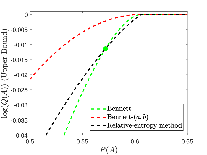
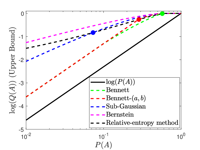
We illustrate these bounds using ambiguity sets constructed from classical MGF-bounds; see Section 2.2 and D. In particular, Figure 4 demonstrates the ambiguity set inclusions from Lemmas D4 - D7, and also compares the risk-sensitive and non-risk-sensitive bounds. In the non-risk-sensitive bound (88) we use the bound on R(Q∥P)R(Q\|P) that is implied by Q∈𝒰Λ​(P)Q\in\mathcal{U}^{\Lambda}(P), as discussed in Lemma 2.4. The Bennett-bound, which utilizes an upper bound on log⁡(d​Q/d​P)\log(dQ/dP) as well as its mean and variance under QQ, is the tightest among the risk-sensitive bounds; this is a consequence of the Lemmas in D. For each risk-sensitive bound there is a crossover level of rarity, below which it becomes tighter than the non-risk-sensitive bound. This is a commonly observed occurrence when comparing the methods: the Rényi-divergence based methods generally perform better for sufficiently rare events, but for more typical events, the relative-entropy-based method from Proposition 5.8 is preferable. In practice, it is of little additional cost to compute both bounds (87) and (88) and use the minimum of the two.

Refer to caption
Refer to caption
Refer to caption
Figure 4: Comparison of the non-risk-sensitive UQ upper bound (i.e., relative-entropy-based bound) from Eq. (84) (black dashed curves) with the risk-sensitive UQ upper bounds from Eq. (86). We show plots over several different ranges of P⁡(A)P(A) and comparison of various ambiguity-set types defined in D. These plots illustrate the following: for each risk-sensitive bound there is a crossover level of rarity (shown by the circles of the corresponding color), below which it becomes tighter than the non-risk-sensitive bound. Intuitively, the relative-entropy-based method is superior for ‘typical events’ (P⁡(A)P(A) close to 11), but the Rényi-based bounds are tighter for sufficiently rare events. The parameter values used are as follows: b=1b=1, a=−1a=-1, η=1/2\eta=1/2, σ2=(b−η)​(η−a)/8\sigma^{2}=(b-\eta)(\eta-a)/8 (for the Bennett ambiguity set), M=1M=1, with the variance for the sub-Gaussian ambiguity set chosen as in the inclusion from Lemma D6.

6 Properties of the Risk-Sensitive UQ Bounds

This section contains several properties new properties, of both theoretical and computational interest, regarding to the UQ bounds in Lemma 5.6. First, we state the divergence property and then we give various tightness results; proofs can be found in the appendices.

6.1 Divergence Property

The UQ bound from Lemma 5.6 can alternatively be formulated in terms of what we call the goal-oriented Rényi divergences. For simplicity, in this subsection we focus on the case τ=eg\tau=e^{g} with g∈B⁡(Ω)g\in B(\Omega).

Theorem 6.1 (Goal-Oriented Rényi Divergence).

Let P,QP,Q be probability measures on (Ω,ℳ)(\Omega,\mathcal{M}) and g∈B⁡(Ω)g\in B(\Omega). Then for γ∈ℝ∖{0}\gamma\in\mathbb{R}\setminus\{0\} we have

1γ​log​[∫eγ​g​𝑑Q]−1γ​log​[∫eγ​g​𝑑P]\displaystyle\frac{1}{\gamma}\log\left[\int e^{\gamma g}dQ\right]-\frac{1}{\gamma}\log\left[\int e^{\gamma g}dP\right] (89)
≤\displaystyle\leq infβ>γ,β≠0{1βlog[∫eβ​gdP]−1γlog[∫eγ​gdP]+1β−γRβ/(β−γ)(Q∥P)}≡Ξ+γ(Q∥P,g)\displaystyle\inf_{\beta>\gamma,\beta\neq 0}\left\{\frac{1}{\beta}\log\left[\int e^{\beta g}dP\right]-\frac{1}{\gamma}\log\left[\int e^{\gamma g}dP\right]+\frac{1}{\beta-\gamma}R_{\beta/(\beta-\gamma)}(Q\|P)\right\}\equiv\Xi^{\gamma}_{+}(Q\|P,g)

and

1γ​log​[∫eγ​g​𝑑Q]−1γ​log​[∫eγ​g​𝑑P]\displaystyle\frac{1}{\gamma}\log\left[\int e^{\gamma g}dQ\right]-\frac{1}{\gamma}\log\left[\int e^{\gamma g}dP\right] (90)
≥\displaystyle\geq supβ<γ,β≠0{1βlog[∫eβ​gdP]−1γlog[∫eγ​gdP]−1γ−βRγ/(γ−β)(P∥Q)}≡Ξ−γ(Q∥P,g).\displaystyle\sup_{\beta<\gamma,\beta\neq 0}\left\{\frac{1}{\beta}\log\left[\int e^{\beta g}dP\right]-\frac{1}{\gamma}\log\left[\int e^{\gamma g}dP\right]-\frac{1}{\gamma-\beta}R_{\gamma/(\gamma-\beta)}(P\|Q)\right\}\equiv\Xi^{\gamma}_{-}(Q\|P,g).

Ξ±γ\Xi_{\pm}^{\gamma} have the following properties:

  1. 1.
    Ξ−γ(Q∥P,g)=−Ξ+−γ(Q∥P,−g).\Xi_{-}^{\gamma}(Q\|P,g)=-\Xi_{+}^{-\gamma}(Q\|P,-g). (91)
  2. 2.

    Divergence property:

    ±Ξ±γ(Q∥P,g)≥0,\pm\Xi_{\pm}^{\gamma}(Q\|P,g)\geq 0, (92)

    and if gg is not PP-a.s. constant then equality holds in Eq. (92) iff Q=PQ=P. (Note that only one of Ξ±γ(Q∥P,g)\Xi_{\pm}^{\gamma}(Q\|P,g) must be zero to guarantee that Q=PQ=P.)

Remark 6.2.

We call Ξ±γ\Xi_{\pm}^{\gamma} the goal-oriented Rényi divergences. The term goal-oriented refers to the fact that the divergences incorporate information about the QoI, gg.

6.2 Tightness Properties

Next, we show that the bounds in Lemma 5.6 satisfy a pair of tightness properties. First, we show that for a given τ\tau, we have tightness over a particular range of QQ’s. The proof follows by combining the UQ bound from Lemma 5.6 with explicit calculations using Eq. (10); see C for a detailed proof.

Theorem 6.3.

Let PP be a probability measure on (Ω,ℳ)(\Omega,\mathcal{M}), τ:Ω→[0,∞]\tau:\Omega\to[0,\infty] be measurable, and γ≠0,−1\gamma\neq 0,-1 with 0<EP​[τγ]<∞0<E_{P}[\tau^{\gamma}]<\infty (τγ\tau^{\gamma} denotes the γ\gamma’th power). Define the probability measure

d​Qγ=τγ​d​P/EP​[τγ]dQ_{\gamma}=\tau^{\gamma}dP/E_{P}[\tau^{\gamma}] (93)

and, for any β∈ℝ\beta\in\mathbb{R}, I⊂ℝI\subset\mathbb{R}, define the ambiguity sets

𝒰βγ(P)={Q:Rβ(Q∥P)≤Rβ(Qγ∥P)},\displaystyle\mathcal{U}^{\gamma}_{\beta}(P)=\{Q:R_{\beta}(Q\|P)\leq R_{\beta}(Q_{\gamma}\|P)\}, (94)
𝒰Iγ(P)={Q:Rα(Q∥P)≤Rα(Qγ∥P) for all α∈I},\displaystyle\mathcal{U}_{I}^{\gamma}(P)=\{Q:R_{\alpha}(Q\|P)\leq R_{\alpha}(Q_{\gamma}\|P)\,\text{ for all }\,\alpha\in I\},

i.e., ambiguity sets of the form Eq. (12) with h(α)=Rα(Qγ∥P)h(\alpha)=R_{\alpha}(Q_{\gamma}\|P), either just for α=β\alpha=\beta or for all α∈I\alpha\in I.

Then

Qγ∈𝒰Iγ​(P)⊂𝒰βγ​(P)​ for any β∈I\displaystyle Q_{\gamma}\in\mathcal{U}_{I}^{\gamma}(P)\subset\mathcal{U}^{\gamma}_{\beta}(P)\,\text{ for any $\beta\in I$ } (95)

and:

  1. 1.

    If γ>0\gamma>0 we have

    supQ∈𝒰(1,∞)γ​(P)log⁡[∫τ​𝑑Q]=supQ∈𝒰1+γ−1γ​(P)log⁡[∫τ​𝑑Q]=\displaystyle\sup_{Q\in\mathcal{U}^{\gamma}_{(1,\infty)}(P)}\log\left[\int\tau dQ\right]=\sup_{Q\in\mathcal{U}^{\gamma}_{1+\gamma^{-1}}(P)}\log\left[\int\tau dQ\right]= log⁡[∫τ​d​Qγ]\displaystyle\log\left[\int\tau dQ_{\gamma}\right] (96)
    =\displaystyle= infc>1{1clog[∫τcdP]+1c−1Rc/(c−1)(Qγ∥P)},\displaystyle\inf_{c>1}\left\{\frac{1}{c}\log\left[\int\tau^{c}dP\right]+\frac{1}{c-1}R_{c/(c-1)}(Q_{\gamma}\|P)\right\},

    and the infimum is achieved at c=γ+1c=\gamma+1.

  2. 2.

    If γ∈(−1,0)\gamma\in(-1,0), τ<∞\tau<\infty PP-a.s., and EP​[τγ+1]<∞E_{P}[\tau^{\gamma+1}]<\infty then

    infQ∈𝒰(−∞,0)γ​(P)log⁡[∫τ​𝑑Q]=infQ∈𝒰1+γ−1γ​(P)log⁡[∫τ​𝑑Q]=\displaystyle\inf_{Q\in\mathcal{U}^{\gamma}_{(-\infty,0)}(P)}\log\left[\int\tau dQ\right]=\inf_{Q\in\mathcal{U}^{\gamma}_{1+\gamma^{-1}}(P)}\log\left[\int\tau dQ\right]= log⁡[∫τ​d​Qγ]\displaystyle\log\left[\int\tau dQ_{\gamma}\right] (97)
    =\displaystyle= supc<1,c≠0{1clog[∫τcdP]−11−cR1/(1−c)(P||Qγ)},\displaystyle\sup_{c<1,c\neq 0}\left\{\frac{1}{c}\log\left[\int\tau^{c}dP\right]-\frac{1}{1-c}R_{1/(1-c)}(P||Q_{\gamma})\right\},

    and the supremum is achieved at c=γ+1c=\gamma+1.

  3. 3.

    If γ<−1\gamma<-1 we have

    infQ∈𝒰(0,1)γ​(P)log⁡[∫τ​𝑑Q]=infQ∈𝒰1+γ−1γ​(P)log⁡[∫τ​𝑑Q]=\displaystyle\inf_{Q\in\mathcal{U}^{\gamma}_{(0,1)}(P)}\log\left[\int\tau dQ\right]=\inf_{Q\in\mathcal{U}^{\gamma}_{1+\gamma^{-1}}(P)}\log\left[\int\tau dQ\right]= log⁡[∫τ​d​Qγ]\displaystyle\log\left[\int\tau dQ_{\gamma}\right] (98)
    =\displaystyle= supc<1,c≠0{1clog[∫τcdP]−11−cR1/(1−c)(P||Qγ)},\displaystyle\sup_{c<1,c\neq 0}\left\{\frac{1}{c}\log\left[\int\tau^{c}dP\right]-\frac{1}{1-c}R_{1/(1-c)}(P||Q_{\gamma})\right\},

    and the supremum is achieved at c=γ+1c=\gamma+1.

Remark 6.4.

Theorem 6.3 shows that, for fixed PP and τ\tau, tightness of the UQ bounds in Lemma 5.6 holds over the ambiguity set of the form Eq. (12) that is constructed from h(α)=Rα(Qγ∥P)h(\alpha)=R_{\alpha}(Q_{\gamma}\|P) for an appropriate range of α∈I\alpha\in I (II being related to γ\gamma as stated in the above theorem).

We also obtain a tightness result over a range of QoIs, for fixed PP and QQ. The method of proof is very similar to the proof of Theorem 6.3; see C for details.

Theorem 6.5.

Let PP and QQ be probability measures on (Ω,ℳ)(\Omega,\mathcal{M}). For ρ:Ω→[0,∞]\rho:\Omega\to[0,\infty] measurable, define

𝒯β+(ρ)={τ:Ω→[0,∞]|τ is measurable and EP[τβ]≤EP[ρβ]},β≠0,\displaystyle\mathcal{T}^{+}_{\beta}(\rho)=\left\{\tau:\Omega\to[0,\infty]|\tau\text{ is measurable and }E_{P}[\tau^{\beta}]\leq E_{P}[\rho^{\beta}]\right\},\,\,\,\beta\neq 0, (99)
𝒯β−(ρ)={τ:Ω→[0,∞]|τ is measurable and EP[τβ]≥EP[ρβ]},β≠0.\displaystyle\mathcal{T}^{-}_{\beta}(\rho)=\left\{\tau:\Omega\to[0,\infty]|\tau\text{ is measurable and }E_{P}[\tau^{\beta}]\geq E_{P}[\rho^{\beta}]\right\},\,\,\,\beta\neq 0.
  1. 1.

    Suppose Q≪PQ\ll P. For ν>0\nu>0 define ϕν=(d​Q/d​P)ν\phi_{\nu}=(dQ/dP)^{\nu}.

    Then

    supτ∈𝒯1+ν−1+​(ϕν)log⁡[∫τ​𝑑Q]=\displaystyle\sup_{\tau\in\mathcal{T}^{+}_{1+\nu^{-1}}(\phi_{\nu})}\log\left[\int\tau dQ\right]= log⁡[∫ϕν​𝑑Q]\displaystyle\log\left[\int\phi_{\nu}dQ\right] (100)
    =\displaystyle= infc>1{1clog[∫ϕνcdP]+1c−1Rc/(c−1)(Q∥P)},\displaystyle\inf_{c>1}\left\{\frac{1}{c}\log\left[\int\phi_{\nu}^{c}dP\right]+\frac{1}{c-1}R_{c/(c-1)}(Q\|P)\right\},

    the infimum is achieved at c=1+ν−1c=1+\nu^{-1}, and

    log[∫ϕνdQ]=ν(1+ν)R1+ν(Q∥P).\displaystyle\log\left[\int\phi_{\nu}dQ\right]=\nu(1+\nu)R_{1+\nu}(Q\|P). (101)
  2. 2.

    Suppose P≪QP\ll Q. For ν>1\nu>1 define ρν=(d​P/d​Q)ν\rho_{\nu}=(dP/dQ)^{\nu}. If ∫(𝑑P/𝑑Q)ν−1​𝑑P<∞\int(dP/dQ)^{\nu-1}dP<\infty then

    infτ∈𝒯1−ν−1−​(ρν)log⁡[∫τ​𝑑Q]=\displaystyle\inf_{\tau\in\mathcal{T}^{-}_{1-\nu^{-1}}(\rho_{\nu})}\log\left[\int\tau dQ\right]= log⁡[∫ρν​𝑑Q]\displaystyle\log\left[\int\rho_{\nu}dQ\right] (102)
    =\displaystyle= supc<1,c≠0{1clog[∫ρνcdP]−11−cR1/(1−c)(P∥Q)},\displaystyle\sup_{c<1,c\neq 0}\left\{\frac{1}{c}\log\left[\int\rho_{\nu}^{c}dP\right]-\frac{1}{1-c}R_{1/(1-c)}(P\|Q)\right\},

    the supremum is achieved at c=1−ν−1c=1-\nu^{-1}, and

    log[∫ρνdQ]=ν(ν−1)Rν(P∥Q).\displaystyle\log\left[\int\rho_{\nu}dQ\right]=\nu(\nu-1)R_{\nu}(P\|Q). (103)
  3. 3.

    Suppose P≪QP\ll Q. For ν∈(0,1)\nu\in(0,1) define ρν=(d​P/d​Q)ν\rho_{\nu}=(dP/dQ)^{\nu}. Then

    infτ∈𝒯1−ν−1+​(ρν)log⁡[∫τ​𝑑Q]=\displaystyle\inf_{\tau\in\mathcal{T}^{+}_{1-\nu^{-1}}(\rho_{\nu})}\log\left[\int\tau dQ\right]= log⁡[∫ρν​𝑑Q]\displaystyle\log\left[\int\rho_{\nu}dQ\right] (104)
    =\displaystyle= supc<1,c≠0{1clog[∫ρνcdP]−11−cR1/(1−c)(P∥Q)},\displaystyle\sup_{c<1,c\neq 0}\left\{\frac{1}{c}\log\left[\int\rho_{\nu}^{c}dP\right]-\frac{1}{1-c}R_{1/(1-c)}(P\|Q)\right\},

    the supremum is achieved at c=1−ν−1c=1-\nu^{-1}, and Eq. (103) holds.

Remark 6.6.

One can prove a related tightness property for the KL-divergences: If R(Q∥P)<∞R(Q\|P)<\infty, R(P∥Q)<∞R(P\|Q)<\infty, and for ν>0\nu>0 we define fν±=±ν​log⁡(d​Q/d​P)f^{\pm}_{\nu}=\pm\nu\log(dQ/dP) then

±infc>0{1clog(EP[e±c​fν±])+1cR(Q∥P)}=EQ[fν±]=±νR(Q∥P).\displaystyle\pm\inf_{c>0}\left\{\frac{1}{c}\log\left(E_{P}\left[e^{\pm cf^{\pm}_{\nu}}\right]\right)+\frac{1}{c}R(Q\|P)\right\}=E_{Q}[f^{\pm}_{\nu}]=\pm\nu R(Q\|P). (105)

7 Applications

7.1 Battery Failure Probability

As our first application of the methods developed above, we illustrate the steps one might take in analyzing risk-sensitivity for a model obtained by fitting to a data-set. Specifically, we will analyze the life-time, TT, of lithium-ion batteries using the data set of N=124N=124 battery failure times from [3] (TT is the number of charge-discharge cycles over the battery’s lifetime); see the left pane of Figure 5 for a histogram.

Refer to caption
Refer to caption
Figure 5: Left: Histogram created from the 124 battery lifetimes, TT, in the data-set from [3] (see the supplementary material), together with the gamma-distribution fit and a kernel-density estimator. Right: Upper bounds on the expected battery failure rate, E⁡[1/T]E[1/T], computed using the risk-sensitive UQ bound Eq. (87), under the scenarios of super-exponential decay (blue curve; see Eq. (64) with κ=2\kappa=2), power-law decay (magenta curve; see Eq. (59)), and Gaussian ambiguity set (red curve; see Eq. (68)). The parameter r0r_{0} is related to the relative entropy of the alternative models with respect to the baseline (see Section 4.1 as well as the discussion below). The non-risk-sensitive bound (88), which is based on relative entropy, is not applicable here as the MGF of the QoI does not exist on any neighborhood of 00. The baseline model QoI (black solid line) was computed from a MLE fit to a gamma distribution; see Eq. (106) - (107).

The steps suggested by the framework developed above are as follows:

  1. 1.

    Pick a QoI: If one is interested in risk-sensitive QoIs then the Rényi-based methodology developed in this paper is appropriate (see the discussion in Section 5.3). Here we will study the battery failure rate: τ=1/T\tau=1/T, which is very sensitive to the tail of the distribution near T=0T=0.

  2. 2.

    Construct the Baseline Model from the Data: The chosen QoI is most sensitive to the tail near zero (the ‘early’ failure probability), and is relatively insensitive to the large TT tail. We choose to fit to a gamma distribution, with probability density

    pa,b(T)=1ba​Γ​(a)Ta−1e−T/b,t>0,p_{a,b}(T)=\frac{1}{b^{a}\Gamma(a)}T^{a-1}e^{-T/b},\,\,\,t>0, (106)

    as it provides a dedicated parameter, aa, to fit the decay at 00 (unlike, for example, the Weibull family, where the decay as T→0T\to 0 and T→∞T\to\infty are linked).

    The maximum likelihood estimators (MLE) obtained from the data in [3] are used to define the baseline model:

    P⁡(d​T)=pa,b​(T)​d​T,a≡a^=5.38,b≡b^=149.\displaystyle P(dT)=p_{a,b}(T)dT,\,\,\,\,\,a\equiv\widehat{a}=5.38,\,\,\,b\equiv\widehat{b}=149. (107)
  3. 3.

    Build Ambiguity Set(s): As is apparent form the frequency histogram, Figure 1, the data set contains very little information about the tails of the distribution. The chosen QoI, τ=1/T\tau=1/T, is risk sensitive and so one should have a healthy skepticism regarding the value of EP​[1/T]E_{P}[1/T] that is computed form the model constructed in step (2). It is therefore important to test the robustness of the chosen QoI under perturbations, QQ, of the baseline model PP. Performing a non-parametric robustness test using our methods requires the choice of an ambiguity set, defined via Eq. (16) (or, more concretely, via Eq. (32)). The choice of ambiguity set should reflect the type of model-form uncertainty one wishes to test (i.e., the type of stress test). We discuss this choice in more detail below.

  4. 4.

    Compute Robustness Bounds: Now that we have a QoI and ambiguity set(s), we can use Theorem 5.9 to obtain UQ bounds.

    Remark 7.1.

    Note that the MGF of the QoI τ=1/T\tau=1/T under PP does not exist. This is another indication that the QoI is risk-sensitive and also implies that the non-risk-sensitive bound from Proposition Eq. (5.8) is not applicable in this case. In contrast, the risk-sensitive bound (86) only requires existence of cc’th moments for cc in a neighborhood of 11, and so is applicable in this case. This is an extreme form of the phenomenon seen in Figure 4, where the risk-sensitive UQ bounds were seen to be tighter than the non-risk-sensitive bounds when the degree of risk-sensitivity (rarity) became sufficiently high.

For illustrative purposes, we characterize the system under three tail-decay scenarios, using the framework of Section 3: power-law decay (59), super-exponential decay (Eq. (64) with κ=2\kappa=2), and the Gaussian ambiguity set (Eq. (68)). UQ bounds are shown in the right pane of Figure 5 as a function of r0r_{0}. Each of the corresponding ambiguity sets are fixed once one specifies an upper bound on the relative entropy, as that fixes r0r_{0} in Eq. (62), Eq. (67), or Eq. (71). There is a large body of literature on estimating relative entropy, and other density functionals [20, 21, 22, 23, 24, 25, 26], though none of these works appear to rigorously apply to the task of estimating R(Q∥P)R(Q\|P) in this situation (continuous distributions of unbounded support). Here, we use a bootstrap method, where we take NN samples (with replacement) from the data set, use the sample to form a kernel density estimator and use that as a surrogate for QQ to compute R(Q∥P)R(Q\|P). Averaging the result over many different samples results in R(Q∥P)≈0.074R(Q\|P)\approx 0.074.

Selecting which ambiguity set to use, out of the three types shown in Figure 5 (or out of the infinitely many other possibilities), is a modeling choice; each such choice represents a different type of stress-test of the model. Given that we have little data regarding the tail at 00, it is reasonable to stress-test the model via alternative models that decay polynomially at 00 with a slower rate β\beta, than the MLE fit, i.e., β<a\beta<a. Thinking of the tail near zero, such alternative models with have log-likelihood decay of the form:

P(dQ/dP≥r)≈P(CTβ−1/Ta−1≥r)≈Dr−a/(a−β)\displaystyle P(dQ/dP\geq r)\approx P(CT^{\beta-1}/T^{a-1}\geq r)\approx Dr^{-a/(a-\beta)} (108)

for rr large enough (CC, DD are some constants). This is of the power-law type (59).

Remark 7.2.

Note that here, power-law decay of the likelihood under PP does correspond to power-law perturbation of the density near 00. This is because PP also has a power-law form near 00.

Therefore, we are motivated to stress-test the model under the power-law family of ambiguity sets (59). This, together with the estimate R(Q∥P)≈0.074R(Q\|P)\approx 0.074, fixes r0≈0.70r_{0}\approx 0.70. The resulting UQ bound obtained from Theorem 5.9 (see Figure 5) is EQ​[1/T]≤0.00194E_{Q}[1/T]\leq 0.00194 for all Q∈𝒰r0P​L​(P)Q\in\mathcal{U}^{PL}_{r_{0}}(P), as compared to the base-model expectation EP​[1/T]=0.00153E_{P}[1/T]=0.00153. We emphasize that we do not simply compute the QoI under the gamma distribution Eq. (106) with perturbed values of aa; our goal with these methods is to obtain robust UQ bounds over non-parametric model neighborhoods.

Remark 7.3.

We obtain a very similar bound EQ​[1/T]≤0.00198E_{Q}[1/T]\leq 0.00198, if we stress-test via the Gaussian ambiguity set (see Eq. (68)). Based on the discussion in Remark 4.1, this is unsurprising.

7.2 Distributional Robustness for Large Deviations Rate Functions

Next, we show how our results can yield UQ bounds on large deviations rate functions. Specifically, we let XnX_{n}, n∈ℤ+n\in\mathbb{Z}^{+} be IID ℝd\mathbb{R}^{d}-valued random variables with distribution PP and finite MGF everywhere, i.e.,

∫ev⋅x​P​(𝑑x)<∞,v∈ℝd.\displaystyle\int e^{v\cdot x}P(dx)<\infty,\,\,\,v\in\mathbb{R}^{d}. (109)

Let PnP_{n} be the distribution of X¯n≡1n​∑i=1nXi\overline{X}_{n}\equiv\frac{1}{n}\sum_{i=1}^{n}X_{i}. Cramer’s Theorem (see, for example, Section 2.2 in [13]) implies that the PnP_{n} satisfy a large deviations principle with rate function, IPI_{P}, given by

IP​(x)=supv∈ℝd{v⋅x−ΛP​(v)},ΛP​(v)≡log⁡[∫ev⋅y​P​(𝑑y)].\displaystyle I_{P}(x)=\sup_{v\in\mathbb{R}^{d}}\left\{v\cdot x-\Lambda_{P}(v)\right\},\,\,\,\Lambda_{P}(v)\equiv\log\left[\int e^{v\cdot y}P(dy)\right]. (110)

In the following result, we obtain UQ bounds on this type of rate function:

Theorem 7.4.

Let P,QP,Q be probability measures on ℝd\mathbb{R}^{d}. Then, using the definitions from Eq. (110), we have

supc>1{1cIP(x)−1c−1Rc/(c−1)(Q∥P)}≤IQ(x)≤inf0<c<1{1cIP(x)+11−cR1/(1−c)(P∥Q)}\displaystyle\sup_{c>1}\left\{\frac{1}{c}I_{P}(x)-\frac{1}{c-1}R_{c/(c-1)}(Q\|P)\right\}\leq I_{Q}(x)\leq\inf_{0<c<1}\left\{\frac{1}{c}I_{P}(x)+\frac{1}{1-c}R_{1/(1-c)}(P\|Q)\right\} (111)

(∞−∞≡−∞\infty-\infty\equiv-\infty in the lower bound).

Proof.

Lemma 5.6 with τ⁡(x)=ev⋅x\tau(x)=e^{v\cdot x} gives

ΛQ(v)≤infc>1{1clog[∫ec​v⋅yP(dy)]+1c−1Rc/(c−1)(Q∥P)}.\displaystyle\Lambda_{Q}(v)\leq\inf_{c>1}\left\{\frac{1}{c}\log\left[\int e^{cv\cdot y}P(dy)\right]+\frac{1}{c-1}R_{c/(c-1)}(Q\|P)\right\}. (112)

Therefore, for c>1c>1,

IQ​(x)≥\displaystyle I_{Q}(x)\geq 1csupv∈ℝd{cv⋅x−log[∫ec​v⋅yP(dy)]}−1c−1Rc/(c−1)(Q∥P)\displaystyle\frac{1}{c}\sup_{v\in\mathbb{R}^{d}}\left\{cv\cdot x-\log\left[\int e^{cv\cdot y}P(dy)\right]\right\}-\frac{1}{c-1}R_{c/(c-1)}(Q\|P) (113)
=\displaystyle= 1cIP(x)−1c−1Rc/(c−1)(Q∥P).\displaystyle\frac{1}{c}I_{P}(x)-\frac{1}{c-1}R_{c/(c-1)}(Q\|P).

Taking the supremum over c>1c>1 gives the lower bound.

The derivation of the upper bound proceeds similarly:

ΛQ​(v)≥\displaystyle\Lambda_{Q}(v)\geq supc<1,c≠0{1clog[∫ec​v⋅yP(dy)]−11−cR1/(1−c)(P∥Q)}\displaystyle\sup_{c<1,c\neq 0}\left\{\frac{1}{c}\log\left[\int e^{cv\cdot y}P(dy)\right]-\frac{1}{1-c}R_{1/(1-c)}(P\|Q)\right\} (114)

( ∞−∞≡−∞\infty-\infty\equiv-\infty). So for 0<c<10<c<1 we have

IQ​(x)≤\displaystyle I_{Q}(x)\leq 1csupv∈ℝd{v⋅x−log[∫ev⋅yP(dy)]}+11−cR1/(1−c)(P∥Q)\displaystyle\frac{1}{c}\sup_{v\in\mathbb{R}^{d}}\left\{v\cdot x-\log\left[\int e^{v\cdot y}P(dy)\right]\right\}+\frac{1}{1-c}R_{1/(1-c)}(P\|Q) (115)
=\displaystyle= 1cIP(x)+11−cR1/(1−c)(P∥Q).\displaystyle\frac{1}{c}I_{P}(x)+\frac{1}{1-c}R_{1/(1-c)}(P\|Q).

(Note that we must restrict the supremum to c>0c>0 so that we can pull the 1/c1/c factor out of the supremum.) Taking the infimum over c∈(0,1)c\in(0,1) gives the upper bound.

As a concrete example, let PP be a normal distribution on ℝd\mathbb{R}^{d} with mean 00 and invertible covariance matrix Σ\Sigma; the associated rate function is IP​(x)=12​x​Σ−1​xI_{P}(x)=\frac{1}{2}x\Sigma^{-1}x. Suppose we are considering a specific alternative model

Q⁡(d​x)=Z−1​(1+ϕ⁡(x))​P​(d​x),\displaystyle Q(dx)=Z^{-1}(1+\phi(x))P(dx), (116)

e.g., a ‘rough’ non-Gaussian perturbation ϕ\phi, where ZZ is the normalization factor and we assume known bounds 0<m≤1+ϕ⁡(x)≤M0<m\leq 1+\phi(x)\leq M for all xx.

Here we illustrate the use of the classical MGF bounds (in particular, the Bennett bound) that were discussed at the end of Section 2.2: The assumed bounds on 1+ϕ1+\phi imply

a≡\displaystyle a\equiv log⁡(m/M)≤log⁡(m/Z)≤log⁡(d​Q/d​P)≤log⁡(M/Z)≤log⁡(M/m)≡b,\displaystyle\log(m/M)\leq\log(m/Z)\leq\log(dQ/dP)\leq\log(M/Z)\leq\log(M/m)\equiv b, (117)

(note that a=−ba=-b) and so the Bennett bound Eq. (21) combined with Eq. (14) gives

Rα(Q∥P)≤1α⁡(α−1)((α−1)b+log((b−η)2(b−η)2+σ2e−(α−1)​(σ2/(b−η)+(b−η))+σ2(b−η)2+σ2))≡h(α),α>1,\displaystyle R_{\alpha}(Q\|P)\leq\frac{1}{\alpha(\alpha-1)}\left((\alpha-1)b+\log\left(\frac{(b-\eta)^{2}}{(b-\eta)^{2}+\sigma^{2}}e^{-(\alpha-1)(\sigma^{2}/(b-\eta)+(b-\eta))}+\frac{\sigma^{2}}{(b-\eta)^{2}+\sigma^{2}}\right)\right)\equiv h(\alpha),\,\,\,\alpha>1, (118)

where η≤b\eta\leq b is an upper bound on R(Q∥P)R(Q\|P) and σ2\sigma^{2} is an upper bound on VarQ⁡[log⁡(d​Q/d​P)]\operatorname{Var}_{Q}[\log(dQ/dP)]. Eq. (118) can be used in conjunction with Eq. (111) to obtain a lower bound on the rate function. Results are shown in Figure 6 for several values of η\eta and σ2\sigma^{2}. For comparison, we also show the naive bound (black dashed curve) IQ​(x)≥max⁡{IP​(x)−log⁡(M/m),0}I_{Q}(x)\geq\max\{I_{P}(x)-\log(M/m),0\}, obtained from using the upper bound (117) on d​Q/d​PdQ/dP in the definition Eq. (110), together with the fact that rate functions are non-negative.
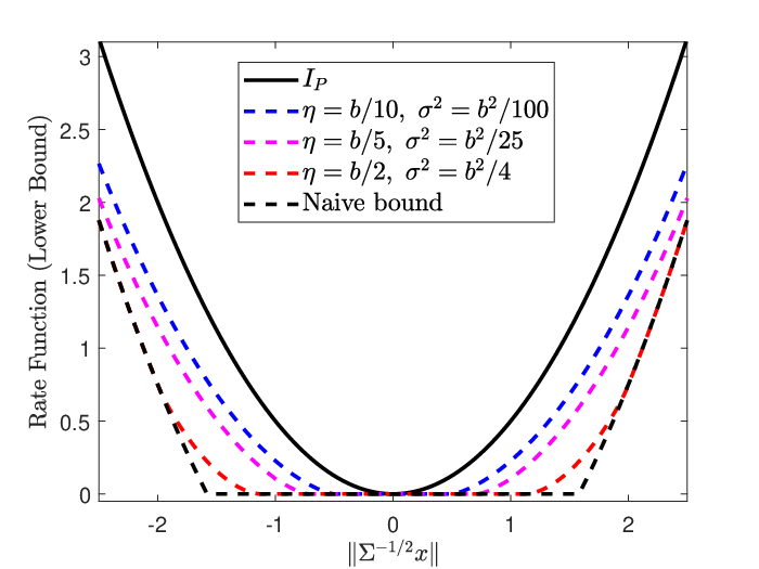
Refer to caption
Figure 6: Lower bounds on the rate function for QQ, computed from Eq. (110). The base model is normal, P=N⁡(0,Σ)P=N(0,\Sigma), with rate function shown in black. We assume a bounded perturbation with −b≤log⁡(d​Q/d​P)≤b=2-b\leq\log(dQ/dP)\leq b=2 and several values of η=R(Q∥P)\eta=R(Q\|P) and σ2=VarQ⁡[log⁡(d​Q/d​P)]\sigma^{2}=\operatorname{Var}_{Q}[\log(dQ/dP)].

To understand the behavior in this figure, note that when ∥Σ−1/2x∥\|\Sigma^{-1/2}x\| is large, the optimum value of cc in the lower bound from Eq. (111) will occur for c≈1c\approx 1, and so α≫1\alpha\gg 1 in Eq. (118). Therefore the upper bound on Rα(Q∥P)R_{\alpha}(Q\|P) will approach b/αb/\alpha, and the optimum value is approximately

1c∗IP(x)−1c∗−1Rc∗/(c∗−1)(Q∥P)\displaystyle\frac{1}{c^{*}}I_{P}(x)-\frac{1}{c^{*}-1}R_{c^{*}/(c^{*}-1)}(Q\|P) (119)
≈\displaystyle\approx 1c∗​(IP​(x)−b)≈IP​(x)−b,\displaystyle\frac{1}{c^{*}}(I_{P}(x)-b)\approx I_{P}(x)-b,

the same result as the naive bound. Hence, all of the bounds converge to the naive bound for ‖Σ−1​x‖\|\Sigma^{-1}x\| sufficiently large. However, for intermediate values of ‖Σ−1​x‖\|\Sigma^{-1}x\| our bounds are much more informative; they do require the additional effort of computing (estimating) R(Q∥P)R(Q\|P) and VarQ⁡[log⁡(d​Q/d​P)]\operatorname{Var}_{Q}[\log(dQ/dP)]. Note that if one can also more accurately estimate ZZ, then a further improvement is be obtained by using b=log⁡(M/Z)b=\log(M/Z).

7.3 Risk-Sensitive Distributionally Robust Optimization with an Application to Option Pricing

Finally, as an application of the tightness results from Section 6.2, we study a distributionally robust optimization (DRO) problem. DRO is an area with much recent work [27, 28, 29, 30, 31, 32, 33, 34, 35], wherein both information-theoretic and optimal-transport (Wasserstein-metric) based methods are widely used. In this section, we develop a DRO result applicable to risk-sensitive QoIs, using Rényi divergences.

The general setting is as follows: Fix a probability measure PP, a collection of QoIs τy:Ω→[0,∞]\tau_{y}:\Omega\to[0,\infty], y∈Yy\in Y (the parameter-space to be optimized over), and ambiguity sets 𝒰y⊂𝒫⁡(Ω)\mathcal{U}^{y}\subset\mathcal{P}(\Omega), y∈Yy\in Y. The goal in risk-sensitive distributionally robust optimization (DRO) is to compute one of the following:

arg​miny∈YsupQ∈𝒰ylogEQ[τy] or arg​maxy∈YinfQ∈𝒰ylogEQ[τy].\displaystyle\argmin_{y\in Y}\sup_{Q\in\mathcal{U}^{y}}\log E_{Q}[\tau_{y}]\,\,\,\,\text{ or }\,\,\,\,\argmax_{y\in Y}\inf_{Q\in\mathcal{U}^{y}}\log E_{Q}[\tau_{y}]. (120)

In the former, τy\tau_{y} is often thought of as a cost, and the latter as a profit; in either case, yy is a design or control variable. The problem Eq. (120) then corresponds to finding the value of the control variable that minimizes (resp. maximizes) the worst case cost (resp. profit) over the ambiguity sets 𝒰y\mathcal{U}^{y}.

Remark 7.5.

The inclusion of the log in Eq. (120) doesn’t impact the minimizer/maximizer, but formulating the problem this way better connects with the results developed above. We need to treat the min-max and max-min problems separately, as our risk-sensitive UQ results only apply to non-negative QoIs, and hence we cannot use the standard technique of converting between the problem types simply by changing the sign of the QoI.

Theorem 6.3 gives conditions under which one can explicitly evaluate the inner maximization or minimization in Eq. (120), for specific classes of ambiguity sets. As a simple, concrete example, we consider the pricing of perpetual American put options. For background see Chapter 8 of [36] or Chapter 8 of [37].

Under the baseline model, the asset price evolves according to geometric Brownian motion in an interest rate-rr environment and with volatility σ\sigma,

d​Xt=r​Xr​d​t+σ​Xt​d​Wt,\displaystyle dX_{t}=rX_{r}dt+\sigma X_{t}dW_{t}, (121)

where r,σ>0r,\sigma>0 are constants. This has the explicit solution

Xt=X0​exp⁡(σ​W​(t)+(r−σ2/2)​t).\displaystyle X_{t}=X_{0}\exp\left(\sigma W(t)+(r-\sigma^{2}/2)t\right). (122)

The baseline measure, PP, is then the distribution of XX on path space, C⁡([0,∞),ℝ)C([0,\infty),\mathbb{R}).

The quantity of interest we consider is defined as follows: Let K>0K>0 be the option strike price. The payout if the option is exercised at time t≥0t\geq 0 is K−xtK-x_{t}, where xtx_{t} is the asset price at time tt. The relevant QoI is then the value, discounted to the present time:

V​[x]t=e−r​t​(K−xt)​1t<∞.\displaystyle V[x]_{t}=e^{-rt}(K-x_{t})1_{t<\infty}. (123)

We assume that the option-holder’s strategy is to exercise the option when the stock price hits some level LL, assumed to satisfy 0<L<K<X00<L<K<X_{0}, i.e., we consider the stopping times τL​[x]=inf{t≥0:xt≤L}\tau_{L}[x]=\inf\{t\geq 0:x_{t}\leq L\}. The option holder’s goal is to choose LL so as to maximize the expected option value at the stopping time, i.e., maximize EP​[VτL]E_{P}[V_{\tau_{L}}]. However, due to lack of confidence in the model, one might desire to build in a safety margin by first maximizing over some ambiguity set of alternative models. With this as motivation, our goal here is to compute the following:

arg​maxLinfQ∈𝒰log(EQ[VL]),VL[x]≡e−r​τL(K−xτL)1τL<∞=(K−L)e−r​τL1τL<∞\displaystyle\argmax_{L}\inf_{Q\in\mathcal{U}}\log(E_{Q}[V_{L}]),\,\,\,\,\,V_{L}[x]\equiv e^{-r\tau_{L}}(K-x_{\tau_{L}})1_{\tau_{L}<\infty}=(K-L)e^{-r\tau_{L}}1_{\tau_{L}<\infty} (124)

for an appropriate ambiguity set 𝒰\mathcal{U} (to be discussed below).

From Eq. (122), one can see that τL\tau_{L} is the level aLa_{L} hitting time of a Brownian motion with constant drift μ\mu, where

aL≡−σ−1​log⁡(X0/L),μ≡r/σ−σ/2.\displaystyle a_{L}\equiv-\sigma^{-1}\log(X_{0}/L),\,\,\,\,\,\,\mu\equiv r/\sigma-\sigma/2. (125)

From Eq. (97), we see that if we choose γ<0,γ≠−1\gamma<0,\gamma\neq-1 and

𝒰=𝒰1+γ−1γ(P)={Q:R1+γ−1(Q∥P)≤R1+γ−1(Qγ∥P)},dQγ≡VLγdP/EP[VLγ]\displaystyle\mathcal{U}=\mathcal{U}^{\gamma}_{1+\gamma^{-1}}(P)=\{Q:R_{1+\gamma^{-1}}(Q\|P)\leq R_{1+\gamma^{-1}}(Q_{\gamma}\|P)\},\,\,\,dQ_{\gamma}\equiv V_{L}^{\gamma}dP/E_{P}[V_{L}^{\gamma}] (126)

(VLγV_{L}^{\gamma} denotes the γ\gamma’th power) then the inner minimization is computable, and we obtain

arg​maxLinfQ∈U1+γ−1γ​(P)log(EQ[VL])=arg​maxLlog(EQγ[VL])=arg​maxLEQγ[VL].\displaystyle\argmax_{L}\inf_{Q\in U^{\gamma}_{1+\gamma^{-1}}(P)}\log(E_{Q}[V_{L}])=\argmax_{L}\log(E_{Q_{\gamma}}[V_{L}])=\argmax_{L}E_{Q_{\gamma}}[V_{L}]. (127)

To make the above calculation valid, we must restrict to parameter values where μ<0\mu<0, so that τL<∞\tau_{L}<\infty PP-a.s. (see Chapter 8 of [36] and page 196 in [38]), otherwise we will have EP​[VLγ]=∞E_{P}[V_{L}^{\gamma}]=\infty.

The expectation can be evaluated using the formula for the MGF of τL\tau_{L} under PP (again, see Chapter 8 of [36]):

EP[e−λ​τL]=exp(aLμ−|aL|μ2+2​λ),λ>−μ2/2.\displaystyle E_{P}[e^{-\lambda\tau_{L}}]=\exp(a_{L}\mu-|a_{L}|\sqrt{\mu^{2}+2\lambda}),\,\,\,\,\lambda>-\mu^{2}/2. (128)

Using this we find for 0>γ>−μ2/(2r)0>\gamma>-\mu^{2}/(2r), γ≠−1\gamma\neq-1:

EQγ​[VL]=\displaystyle E_{Q_{\gamma}}[V_{L}]= ∫VL1+γ​𝑑P/EP​[VLγ]=(K−L)​∫e−r⁡(1+γ)​τL​𝑑P/∫e−r​γ​τL​𝑑P\displaystyle\int V_{L}^{1+\gamma}dP/E_{P}[V_{L}^{\gamma}]=(K-L)\int e^{-r(1+\gamma)\tau_{L}}dP/\int e^{-r\gamma\tau_{L}}dP (129)
=\displaystyle= (K−L)​exp⁡(−|aL|​μ2+2​r​(1+γ)+|aL|​μ2+2​r​γ)\displaystyle(K-L)\exp(-|a_{L}|\sqrt{\mu^{2}+2r(1+\gamma)}+|a_{L}|\sqrt{\mu^{2}+2r\gamma})
=\displaystyle= (K−L)​(L/X0)dγ/σ,dγ≡μ2+2​r​(1+γ)−μ2+2​r​γ.\displaystyle(K-L)(L/X_{0})^{d_{\gamma}/\sigma},\,\,\,\,\,d_{\gamma}\equiv\sqrt{\mu^{2}+2r(1+\gamma)}-\sqrt{\mu^{2}+2r\gamma}.

One can calculate R1+γ−1(Qγ∥P)R_{1+\gamma^{-1}}(Q_{\gamma}\|P) explictly, and thereby write the ambiguity set as

𝒰1+γ−1γ(P)={Q:R1+γ−1(Q∥P)≤−γγ+1aLμ+γ2γ+1|aL|μ2+2​(γ+1)​r+γ|aL|μ2+2​r​γ}.\displaystyle\mathcal{U}^{\gamma}_{1+\gamma^{-1}}(P)=\left\{Q:R_{1+\gamma^{-1}}(Q\|P)\leq-\frac{\gamma}{\gamma+1}a_{L}\mu+\frac{\gamma^{2}}{\gamma+1}|a_{L}|\sqrt{\mu^{2}+2(\gamma+1)r}+\gamma|a_{L}|\sqrt{\mu^{2}+2r\gamma}\right\}. (130)

Note that this ambiguity set only constrains Rα(Q∥P)R_{\alpha}(Q\|P) at the single (but γ\gamma-dependent) value of α=1+γ−1\alpha=1+\gamma^{-1}; in the language of Definition 12, the right-hand-side of Eq. (133) defines h⁡(1+γ−1)h(1+\gamma^{-1}), with hh being undefined otherwise.

For a simple example of a class of alternative models that are contained in 𝒰1+γ−1γ​(P)\mathcal{U}^{\gamma}_{1+\gamma^{-1}}(P), one can take QQ to be the distribution of YY in path space, where YtY_{t} solves an SDE of the form

d​Yt=(r+Δ​rt)​Yt​d​t+σ​Yt​d​Wt,\displaystyle dY_{t}=(r+\Delta r_{t})Y_{t}dt+\sigma Y_{t}dW_{t}, (131)

and the process Δ​r\Delta r is bounded on [0,T][0,T] and equals 00 for t>Tt>T. A straightforward application Girsanov’s theorem can then be used to show that

Rα(Q∥P)≤‖Δ​r‖∞22​σ2T, for all α>1.\displaystyle R_{\alpha}(Q\|P)\leq\frac{\|\Delta r\|_{\infty}^{2}}{2\sigma^{2}}T,\,\,\,\text{ for all $\alpha>1$.} (132)

Combining this with the right-hand-side of Eq. (133), we see that

Q∈𝒰1+γ−1γ​(P)​ if ​‖Δ​r‖∞22​σ2​T≤−γγ+1​aL​μ+γ2γ+1​|aL|​μ2+2​(γ+1)​r+γ​|aL|​μ2+2​r​γ.\displaystyle Q\in\mathcal{U}^{\gamma}_{1+\gamma^{-1}}(P)\,\,\,\text{ if }\,\,\,\frac{\|\Delta r\|_{\infty}^{2}}{2\sigma^{2}}T\leq-\frac{\gamma}{\gamma+1}a_{L}\mu+\frac{\gamma^{2}}{\gamma+1}|a_{L}|\sqrt{\mu^{2}+2(\gamma+1)r}+\gamma|a_{L}|\sqrt{\mu^{2}+2r\gamma}. (133)
Remark 7.6.

More general alternative models that (131) are possible, including ones where Δ​r\Delta r has unbounded support, but bounding the Rényi divergences in such cases is a more involved task; we do not enter into the techniques for doing so here, as they are tangential to our primary goal in this paper.

It should also be noted that in more realistic option-pricing models, the option itself has a finite expiration date, TT, and so the problem is naturally posed on a compact time interval. However, analyzing such models is more complex and we do not discuss them further here; see [36] for details.

From Eq. (129), one can compute the maximizer in Eq. (127):

Lγ∗≡arg​maxL⁡EQγ​[VL]=dγ​Kdγ+σ,dγ=μ2+2​r​(1+γ)−μ2+2​r​γ.\displaystyle L^{*}_{\gamma}\equiv\argmax_{L}E_{Q_{\gamma}}[V_{L}]=\frac{d_{\gamma}K}{d_{\gamma}+\sigma},\,\,\,\,d_{\gamma}=\sqrt{\mu^{2}+2r(1+\gamma)}-\sqrt{\mu^{2}+2r\gamma}. (134)

It is important to note that dγd_{\gamma} is decreasing and

limγ↗0Lγ∗=2​r​K2​r+σ2,\displaystyle\lim_{\gamma\nearrow 0}L^{*}_{\gamma}=\frac{2rK}{2r+\sigma^{2}}, (135)

which equals the optimal LL in the non-risk-sensitive formulation of the problem (see 8.3.12 in [36]). Therefore we can interpret γ<0\gamma<0 as the degree of risk-aversion; when γ\gamma decreases below 00, Lγ∗L^{*}_{\gamma} increases, meaning that a more conservative choice of stopping level is considered optimal when one has uncertainty about one’s model.

Appendix A Proof of the Rényi-Donsker-Varadhan Variational Formula

Here we prove the generalization of the Donsker-Varadhan variational formula from Theorem 5.4 and restated below:

Theorem A1 (Rényi-Donsker-Varadhan Variational Formula).

Let P,QP,Q be probability measures on (Ω,ℳ)(\Omega,\mathcal{M}) and α∈ℝ∖{0,1}\alpha\in\mathbb{R}\setminus\{0,1\}. Then

Rα(Q∥P)=supg∈B⁡(Ω){1α−1log[∫e(α−1)​gdQ]−1αlog[∫eα​gdP]}.\displaystyle R_{\alpha}(Q\|P)=\sup_{g\in B(\Omega)}\left\{\frac{1}{\alpha-1}\log\left[\int e^{(\alpha-1)g}dQ\right]-\frac{1}{\alpha}\log\left[\int e^{\alpha g}dP\right]\right\}. (136)

Proof.

If one can show Eq. (136) for all α>1\alpha>1 and all P,QP,Q, then, using the relation Eq. (11) and reindexing g→−gg\to-g in the supremum, one find that Eq. (136) also holds for all α<0\alpha<0. So we only need to consider the cases α∈(0,1)\alpha\in(0,1) and α>1\alpha>1.

Using Eq. (80) with β=α−1\beta=\alpha-1, γ=α\gamma=\alpha, for all g∈B⁡(Ω)g\in B(\Omega) we find

1αlog[∫eα​gdP]≥1α−1log[∫e(α−1)​gdQ]−Rα(Q∥P),\displaystyle\frac{1}{\alpha}\log\left[\int e^{\alpha g}dP\right]\geq\frac{1}{\alpha-1}\log\left[\int e^{(\alpha-1)g}dQ\right]-R_{\alpha}(Q\|P), (137)

and hence

Rα(Q∥P)≥supg∈B⁡(Ω){1α−1log[∫e(α−1)​gdQ]−1αlog[∫eα​gdP]}≡H(Q∥P).\displaystyle R_{\alpha}(Q\|P)\geq\sup_{g\in B(\Omega)}\left\{\frac{1}{\alpha-1}\log\left[\int e^{(\alpha-1)g}dQ\right]-\frac{1}{\alpha}\log\left[\int e^{\alpha g}dP\right]\right\}\equiv H(Q\|P). (138)

To show the reverse inequality, we separate into three cases:

  1. 1.

    α>1\alpha>1 and Q≪̸PQ\not\ll P: We will show H(Q∥P)=∞H(Q\|P)=\infty, which will prove the desired inequality. To do this, take a measurable set AA with P⁡(A)=0P(A)=0 but Q⁡(A)≠0Q(A)\neq 0. Let g=N​1Ag=N1_{A}. Then

    H(Q∥P)≥\displaystyle H(Q\|P)\geq 1α−1​log​∫e(α−1)​g​𝑑Q−1α​log​∫eα​g​𝑑P\displaystyle\frac{1}{\alpha-1}\log\int e^{(\alpha-1)g}dQ-\frac{1}{\alpha}\log\int e^{\alpha g}dP (139)
    =\displaystyle= 1α−1​log⁡(e(α−1)​N​Q​(A)+Q⁡(Ac))−1α​log⁡P⁡(Ac)→∞\displaystyle\frac{1}{\alpha-1}\log\left(e^{(\alpha-1)N}Q(A)+Q(A^{c})\right)-\frac{1}{\alpha}\log P(A^{c})\to\infty

    as N→∞N\to\infty, since α>1\alpha>1.

  2. 2.

    α>1\alpha>1 and Q≪PQ\ll P: In this case we have

    Rα(Q∥P)=1α⁡(α−1)log(∫(dQ/dP)αdP).\displaystyle R_{\alpha}(Q\|P)=\frac{1}{\alpha(\alpha-1)}\log\left(\int(dQ/dP)^{\alpha}dP\right). (140)

    Let fn,m​(x)=x​11/m<x<n+n​1x≥n+1/m​1x≤1/mf_{n,m}(x)=x1_{1/m<x<n}+n1_{x\geq n}+1/m1_{x\leq 1/m} and gn,m=log⁡(fn,m​(d​Q/d​P))g_{n,m}=\log(f_{n,m}(dQ/dP)). These are bounded and measurable and so

    H(Q∥P)≥\displaystyle H(Q\|P)\geq 1α−1​log​∫e(α−1)​gn,m​𝑑Q−1α​log​∫eα​gn,m​𝑑P\displaystyle\frac{1}{\alpha-1}\log\int e^{(\alpha-1)g_{n,m}}dQ-\frac{1}{\alpha}\log\int e^{\alpha g_{n,m}}dP (141)
    =\displaystyle= 1α−1​log​∫fn,m​(𝑑Q/𝑑P)(α−1)​d​Qd​P​𝑑P−1α​log​∫fn,m​(𝑑Q/𝑑P)α​𝑑P.\displaystyle\frac{1}{\alpha-1}\log\int f_{n,m}(dQ/dP)^{(\alpha-1)}\frac{dQ}{dP}dP-\frac{1}{\alpha}\log\int f_{n,m}(dQ/dP)^{\alpha}dP.

    Define fn​(x)=x​1x<n+n​1x≥nf_{n}(x)=x1_{x<n}+n1_{x\geq n}. Using the dominated convergence theorem to take m→∞m\to\infty, we find

    H(Q∥P)≥\displaystyle H(Q\|P)\geq 1α−1​log​∫fn​(𝑑Q/𝑑P)(α−1)​d​Qd​P​𝑑P−1α​log​∫fn​(𝑑Q/𝑑P)α​𝑑P\displaystyle\frac{1}{\alpha-1}\log\int f_{n}(dQ/dP)^{(\alpha-1)}\frac{dQ}{dP}dP-\frac{1}{\alpha}\log\int f_{n}(dQ/dP)^{\alpha}dP (142)
    ≥\displaystyle\geq 1α⁡(α−1)​log​∫fn​(𝑑Q/𝑑P)α​𝑑P.\displaystyle\frac{1}{\alpha(\alpha-1)}\log\int f_{n}(dQ/dP)^{\alpha}dP.

    We have 0≤fn​(d​Q/d​P)↗d​Q/d​P0\leq f_{n}(dQ/dP)\nearrow dQ/dP, and so the monotone convergence theorem gives

    H(Q∥P)≥\displaystyle H(Q\|P)\geq 1α⁡(α−1)log∫(dQ/dP)αdP=Rα(Q∥P).\displaystyle\frac{1}{\alpha(\alpha-1)}\log\int(dQ/dP)^{\alpha}dP=R_{\alpha}(Q\|P). (143)

    This proves the result in this case.

  3. 3.

    α∈(0,1)\alpha\in(0,1): Here, we have

    Rα(Q∥P)=1α⁡(α−1)log(∫p>0qαp1−αdν),\displaystyle R_{\alpha}(Q\|P)=\frac{1}{\alpha(\alpha-1)}\log\left(\int_{p>0}q^{\alpha}p^{1-\alpha}d\nu\right), (144)

    where ν\nu is any sigma-finite positive measure for which d​Q=q​d​νdQ=qd\nu and d​P=p​d​νdP=pd\nu. Define fn,m​(x)f_{n,m}(x) as in the previous case and let gn,m=log⁡(fn,m​(q/p))g_{n,m}=\log(f_{n,m}(q/p)), where q/pq/p is defined to be 00 if q=0q=0 and +∞+\infty if p=0p=0 and q≠0q\neq 0.

    gn,mg_{n,m} are bounded and measurable, hence

    H(Q∥P)≥\displaystyle H(Q\|P)\geq −11−αlog∫e(α−1)​gn,mdQ−1αlog∫eα​gn,mdP\displaystyle-\frac{1}{1-\alpha}\log\int e^{(\alpha-1)g_{n,m}}dQ-\frac{1}{\alpha}\log\int e^{\alpha g_{n,m}}dP (145)
    =\displaystyle= −11−αlog∫fn,m(q/p)α−1qdν−1αlog∫fn,m(q/p)αpdν.\displaystyle-\frac{1}{1-\alpha}\log\int f_{n,m}(q/p)^{\alpha-1}qd\nu-\frac{1}{\alpha}\log\int f_{n,m}(q/p)^{\alpha}pd\nu.

    We can take n→∞n\to\infty using the dominated convergence theorem (here it is critical that α∈(0,1)\alpha\in(0,1)) to get

    H(Q∥P)≥\displaystyle H(Q\|P)\geq −11−αlog∫1max⁡(1/m,q/p)1−αqdν−1αlog∫max(1/m,q/p)αpdν\displaystyle-\frac{1}{1-\alpha}\log\int\frac{1}{\max(1/m,q/p)^{1-\alpha}}qd\nu-\frac{1}{\alpha}\log\int\max(1/m,q/p)^{\alpha}pd\nu (146)
    ≥\displaystyle\geq −11−αlog∫q>0,p>0qαp1−αdν−1αlog∫p>0max(1/m,q/p)αpdν.\displaystyle-\frac{1}{1-\alpha}\log\int_{q>0,p>0}q^{\alpha}p^{1-\alpha}d\nu-\frac{1}{\alpha}\log\int_{p>0}\max(1/m,q/p)^{\alpha}pd\nu.

    (Note that the second term is always finite.)

    We can use the dominated convergence theorem on the second term to obtain

    H(Q∥P)≥\displaystyle H(Q\|P)\geq −11−αlog∫p>0qαp1−αdν−1αlog∫p>0qαp1−αdν\displaystyle-\frac{1}{1-\alpha}\log\int_{p>0}q^{\alpha}p^{1-\alpha}d\nu-\frac{1}{\alpha}\log\int_{p>0}q^{\alpha}p^{1-\alpha}d\nu (147)
    =\displaystyle= 1α⁡(α−1)log∫p>0qαp1−αdν=Rα(Q∥P).\displaystyle\frac{1}{\alpha(\alpha-1)}\log\int_{p>0}q^{\alpha}p^{1-\alpha}d\nu=R_{\alpha}(Q\|P).

This completes the proof.

Appendix B Proof of UQ Bounds for Risk-Sensitive QoIs

Here we prove the UQ bound for risk-sensitive QoIs, Lemma 5.6, extending Proposition 1.3 to gg that are valued in the extended reals:

Proof.

First suppose τ:Ω→[0,∞)\tau:\Omega\to[0,\infty). If ∫τc​𝑑P=∞\int\tau^{c}dP=\infty or Rc/(c−1)(Q∥P)=∞R_{c/(c-1)}(Q\|P)=\infty then Eq. (86) is trivial, so suppose not.

Define τn=1/n​1τ<1/n+τ​1τ≥1/n\tau_{n}=1/n1_{\tau<1/n}+\tau 1_{\tau\geq 1/n}. These are positive and decrease pointwise to τ\tau. Therefore, Proposition 1.3 with g=log⁡(τn)g=\log(\tau_{n}) gives

log∫τndQ≤1clog∫τncdP+1c−1Rc/(c−1)(Q∥P).\displaystyle\log\int\tau_{n}dQ\leq\frac{1}{c}\log\int\tau_{n}^{c}dP+\frac{1}{c-1}R_{c/(c-1)}(Q\|P). (148)

By Fatou’s Lemma we have ∫τ​𝑑Q≤limn∫τn​𝑑Q\int\tau dQ\leq\lim_{n}\int\tau_{n}dQ, therefore

log∫τdQ≤loglimn∫τndQ≤lim infn(1clog∫τncdP+1c−1Rc/(c−1)(Q∥P)).\displaystyle\log\int\tau dQ\leq\log\lim_{n}\int\tau_{n}dQ\leq\liminf_{n}\left(\frac{1}{c}\log\int\tau_{n}^{c}dP+\frac{1}{c-1}R_{c/(c-1)}(Q\|P)\right). (149)

We are in the case where Rc/(c−1)(Q∥P)<∞R_{c/(c-1)}(Q\|P)<\infty and τc∈L1​(P)\tau^{c}\in L^{1}(P). Therefore τnc=1/nc​1τ<1/n+τc​1τ≥1/n≤1+τc∈L1​(P)\tau_{n}^{c}=1/n^{c}1_{\tau<1/n}+\tau^{c}1_{\tau\geq 1/n}\leq 1+\tau^{c}\in L^{1}(P). The dominated convergence theorem then implies ∫τnc​𝑑P→∫τc​𝑑P\int\tau_{n}^{c}dP\to\int\tau^{c}dP and hence

log∫τdQ≤\displaystyle\log\int\tau dQ\leq 1clog∫τcdP+1c−1Rc/(c−1)(Q∥P).\displaystyle\frac{1}{c}\log\int\tau^{c}dP+\frac{1}{c-1}R_{c/(c-1)}(Q\|P). (150)

This proves Eq. (86) when τ:Ω→[0,∞)\tau:\Omega\to[0,\infty).

To prove Eq. (83) for τ\tau valued in [0,∞)[0,\infty) we need to show that

log[∫τdQ]≥1clog∫τcdP−11−cR1/(1−c)(P∥Q)\displaystyle\log\left[\int\tau dQ\right]\geq\frac{1}{c}\log\int\tau^{c}dP-\frac{1}{1-c}R_{1/(1-c)}(P\|Q) (151)

for all c<1c<1, c≠0c\neq 0. If R1/(1−c)(P∥Q)=∞R_{1/(1-c)}(P\|Q)=\infty or ∫τ​𝑑Q=∞\int\tau dQ=\infty this is trivial, so suppose they are both finite.

Define τn\tau_{n} as above. First let c∈(0,1)c\in(0,1):
0≤τn≤1+τ∈L1​(Q)0\leq\tau_{n}\leq 1+\tau\in L^{1}(Q) (in the case we are considering) so the dominated convergence theorem, combined with Proposition 1.3 and Fatou’s Lemma, give

log⁡[∫τ​𝑑Q]=\displaystyle\log\left[\int\tau dQ\right]= limnlog⁡[∫τn​𝑑Q]\displaystyle\lim_{n}\log\left[\int\tau_{n}dQ\right] (152)
≥\displaystyle\geq lim infn(c−1log∫τncdP−1/(1−c)R1/(1−c)(P∥Q))\displaystyle\liminf_{n}\left(c^{-1}\log\int\tau_{n}^{c}dP-1/(1-c)R_{1/(1-c)}(P\|Q)\right)
≥\displaystyle\geq c−1log∫τcdP−1/(1−c)R1/(1−c)(P∥Q).\displaystyle c^{-1}\log\int\tau^{c}dP-1/(1-c)R_{1/(1-c)}(P\|Q).

Similarly, for c<0c<0 we have

log⁡[∫τ​𝑑Q]=\displaystyle\log\left[\int\tau dQ\right]= limnlog⁡[∫τn​𝑑Q]\displaystyle\lim_{n}\log\left[\int\tau_{n}dQ\right] (153)
≥\displaystyle\geq lim supn(1clog∫τncdP−11−cR1/(1−c)(P∥Q))\displaystyle\limsup_{n}\left(\frac{1}{c}\log\int\tau_{n}^{c}dP-\frac{1}{1-c}R_{1/(1-c)}(P\|Q)\right)
≥\displaystyle\geq 1clog∫τcdP−11−cR1/(1−c)(P∥Q),\displaystyle\frac{1}{c}\log\int\tau^{c}dP-\frac{1}{1-c}R_{1/(1-c)}(P\|Q),

where we used τnc≤τc\tau_{n}^{c}\leq\tau^{c}.

Now consider the general case τ:Ω→[0,∞]\tau:\Omega\to[0,\infty]. Applying the above calculations to τm=τ​1τ≤m+m​1τ>m\tau_{m}=\tau 1_{\tau\leq m}+m1_{\tau>m} (which are valued in [0,∞)[0,\infty)) gives

log[∫τmdQ]≤1clog[∫τmcdP]+1c−1Rc/(c−1)(Q∥P),c>1,\displaystyle\log\left[\int\tau_{m}dQ\right]\leq\frac{1}{c}\log\left[\int\tau_{m}^{c}dP\right]+\frac{1}{c-1}R_{c/(c-1)}(Q\|P),\,\,\,c>1, (154)

where we interpret −∞+∞=∞-\infty+\infty=\infty, and

log[∫τmdQ]≥1clog[∫τmcdP]−11−cR1/(1−c)(P∥Q),c<1,c≠0,\displaystyle\log\left[\int\tau_{m}dQ\right]\geq\frac{1}{c}\log\left[\int\tau_{m}^{c}dP\right]-\frac{1}{1-c}R_{1/(1-c)}(P\|Q),\,\,\,c<1,\,\,c\neq 0, (155)

where ∞−∞=−∞\infty-\infty=-\infty.

Taking m→∞m\to\infty via the monotone convergence theorem gives

log[∫τdQ]≤1clog[∫τcdP]+1c−1Rc/(c−1)(Q∥P)\displaystyle\log\left[\int\tau dQ\right]\leq\frac{1}{c}\log\left[\int\tau^{c}dP\right]+\frac{1}{c-1}R_{c/(c-1)}(Q\|P) (156)

for c>1c>1 and

log[∫τdQ]≥1clog[∫τcdP]−11−cR1/(1−c)(P∥Q)\displaystyle\log\left[\int\tau dQ\right]\geq\frac{1}{c}\log\left[\int\tau^{c}dP\right]-\frac{1}{1-c}R_{1/(1-c)}(P\|Q) (157)

for 0<c<10<c<1.

For c<0c<0, the monotone convergence theorem gives

log[∫τdQ]≥lim supm(1clog[∫τmcdP]−11−cR1/(1−c)(P∥Q)),\displaystyle\log\left[\int\tau dQ\right]\geq\limsup_{m}\left(\frac{1}{c}\log\left[\int\tau_{m}^{c}dP\right]-\frac{1}{1-c}R_{1/(1-c)}(P\|Q)\right), (158)

where we use the convention ∞−∞≡−∞\infty-\infty\equiv-\infty. We have τmc↘τc\tau_{m}^{c}\searrow\tau^{c}, hence if ∫τc​𝑑P<∞\int\tau^{c}dP<\infty then τmc≤1+τc∈L1​(P)\tau_{m}^{c}\leq 1+\tau^{c}\in L^{1}(P) and so the dominated convergence theorem implies

log[∫τdQ]≥1clog[∫τcdP]−11−cR1/(1−c)(P∥Q).\displaystyle\log\left[\int\tau dQ\right]\geq\frac{1}{c}\log\left[\int\tau^{c}dP\right]-\frac{1}{1-c}R_{1/(1-c)}(P\|Q). (159)

If ∫τc​𝑑P=∞\int\tau^{c}dP=\infty then the above bound trivially holds. This completes the proof.

Appendix C Proofs of the Divergence and Tightness Properties

The following is a proof of the divergence property, Theorem 6.1:

Proof.

Eq. (89) and Eq. (90) follow directly from Proposition 5.3 and Eq. (91) follows from reindexing β→−β\beta\to-\beta in the infimum.

To prove non-negativity of Ξ+γ\Xi_{+}^{\gamma}, note that the cumulant generating function Λ(c)≡log∫ec​gdP\Lambda(c)\equiv\log\int e^{cg}dP is smooth and convex (strictly convex if gg is not PP-a.s. constant), hence its derivative is non-decreasing. Therefore

1c​Λ​(c)=∫01Λ′​(c​r)​𝑑r.\displaystyle\frac{1}{c}\Lambda(c)=\int_{0}^{1}\Lambda^{\prime}(cr)dr. (160)

is non-decreasing (strictly increasing if gg is not PP-a.s. constant) in cc. This, together with non-negativity of the Rényi divergences, implies Ξ+γ(Q∥P,g)≥0\Xi_{+}^{\gamma}(Q\|P,g)\geq 0.

If Q=PQ=P then Rα(Q∥P)=0R_{\alpha}(Q\|P)=0 for all α\alpha, and so taking β↘γ\beta\searrow\gamma gives Ξ+γ(Q∥P,g)=0\Xi_{+}^{\gamma}(Q\|P,g)=0.

To complete the proof of the divergence property for Ξ+γ\Xi^{\gamma}_{+}, suppose gg is not PP-a.s. constant and Ξ+γ(Q∥P,g)=0\Xi_{+}^{\gamma}(Q\|P,g)=0. By the definition of Ξ+γ\Xi_{+}^{\gamma}, there must exist βn>γ\beta_{n}>\gamma, βn≠0\beta_{n}\neq 0 with

1βnlog[∫eβn​gdP]−1γlog[∫eγ​gdP]+βn−1βnβn−γRβn/(βn−γ)(Q∥P)→0.\displaystyle\frac{1}{\beta_{n}}\log\left[\int e^{\beta_{n}g}dP\right]-\frac{1}{\gamma}\log\left[\int e^{\gamma g}dP\right]+\beta_{n}^{-1}\frac{\beta_{n}}{\beta_{n}-\gamma}R_{\beta_{n}/(\beta_{n}-\gamma)}(Q\|P)\to 0. (161)

The fact that c→1c​Λ​(c)c\to\frac{1}{c}\Lambda(c) is strictly increasing implies that, after taking a subsequence, we have βn↘γ\beta_{n}\searrow\gamma. Therefore

0=\displaystyle 0= limn→∞1βnlog[∫eβn​gdP]−1γlog[∫eγ​gdP]+βn−1βnβn−γRβn/(βn−γ)(Q∥P)\displaystyle\lim_{n\to\infty}\frac{1}{\beta_{n}}\log\left[\int e^{\beta_{n}g}dP\right]-\frac{1}{\gamma}\log\left[\int e^{\gamma g}dP\right]+\beta_{n}^{-1}\frac{\beta_{n}}{\beta_{n}-\gamma}R_{\beta_{n}/(\beta_{n}-\gamma)}(Q\|P) (162)
=\displaystyle= limn→∞βnβn−γRβn/(βn−γ)(Q∥P).\displaystyle\lim_{n\to\infty}\frac{\beta_{n}}{\beta_{n}-\gamma}R_{\beta_{n}/(\beta_{n}-\gamma)}(Q\|P).

By Eq. (9) we see that, if γ>0\gamma>0, the sequence βnβn−γRβn/(βn−γ)(Q∥P)\frac{\beta_{n}}{\beta_{n}-\gamma}R_{\beta_{n}/(\beta_{n}-\gamma)}(Q\|P) is nondecreasing. Combined with Eq. (162) and non-negativity, we find Rβ1/(β1−γ)(Q∥P)=0R_{\beta_{1}/(\beta_{1}-\gamma)}(Q\|P)=0. The divergence property for Rényi, Eq. (8), then gives Q=PQ=P.

If γ<0\gamma<0, first use Eq. (11) to rewrite Eq. (162) as

0=\displaystyle 0= limn→∞βnβn−γRβn/(βn−γ)(Q∥P)=−limn→∞11−βn/γR1/(1−βn/γ)(P∥Q).\displaystyle\lim_{n\to\infty}\frac{\beta_{n}}{\beta_{n}-\gamma}R_{\beta_{n}/(\beta_{n}-\gamma)}(Q\|P)=-\lim_{n\to\infty}\frac{1}{1-\beta_{n}/\gamma}R_{1/(1-\beta_{n}/\gamma)}(P\|Q). (163)

Taking nn large enough that βn<0\beta_{n}<0 we see that n→11−βn/γR1/(1−βn/γ)(P∥Q)n\to\frac{1}{1-\beta_{n}/\gamma}R_{1/(1-\beta_{n}/\gamma)}(P\|Q) is nondecreasing, and so

0=limn→∞11−βnk/γR1/(1−βnk/γ)(P∥Q)≥11−βn1/γR1/(1−βn1/γ)(P∥Q)≥0.\displaystyle 0=\lim_{n\to\infty}\frac{1}{1-\beta_{n_{k}}/\gamma}R_{1/(1-\beta_{n_{k}}/\gamma)}(P\|Q)\geq\frac{1}{1-\beta_{n_{1}}/\gamma}R_{1/(1-\beta_{n_{1}}/\gamma)}(P\|Q)\geq 0. (164)

Hence R1/(1−βn1/γ)(P∥Q)=0R_{1/(1-\beta_{n_{1}}/\gamma)}(P\|Q)=0 and therefore P=QP=Q. Finally, the divergence property for Ξ−γ\Xi_{-}^{\gamma} follows from Eq. (91).

We now prove the tightness results. These calculations are similar to proving the equality case from Proposition 1.3. First we give a proof of Theorem 6.3:

Proof.
  1. 1.

    Let γ>0\gamma>0. Using Eq. (86) from Lemma 5.6, bounding the infimum by the value at c=1+γc=1+\gamma, and then using the definition of 𝒰1+γ−1γ​(P)\mathcal{U}^{\gamma}_{1+\gamma^{-1}}(P) we have

    supQ∈𝒰1+γ−1γ​(P)log⁡[∫τ​𝑑Q]≤\displaystyle\sup_{Q\in\mathcal{U}^{\gamma}_{1+\gamma^{-1}}(P)}\log\left[\int\tau dQ\right]\leq supQ∈𝒰1+γ−1γ​(P)infc>1{1clog[∫τcdP]+1c−1Rc/(c−1)(Q||P)}\displaystyle\sup_{Q\in\mathcal{U}^{\gamma}_{1+\gamma^{-1}}(P)}\inf_{c>1}\left\{\frac{1}{c}\log\left[\int\tau^{c}dP\right]+\frac{1}{c-1}R_{c/(c-1)}(Q||P)\right\} (165)
    ≤\displaystyle\leq supQ∈𝒰1+γ−1γ​(P){11+γlog[∫τ1+γdP]+1γR1+1/γ(Q||P)}\displaystyle\sup_{Q\in\mathcal{U}^{\gamma}_{1+\gamma^{-1}}(P)}\left\{\frac{1}{1+\gamma}\log\left[\int\tau^{1+\gamma}dP\right]+\frac{1}{\gamma}R_{1+1/\gamma}(Q||P)\right\}
    ≤\displaystyle\leq 11+γlog[∫τ1+γdP]+1γR1+1/γ(Qγ||P).\displaystyle\frac{1}{1+\gamma}\log\left[\int\tau^{1+\gamma}dP\right]+\frac{1}{\gamma}R_{1+1/\gamma}(Q_{\gamma}||P).

    Direct calculation, using Eq. (10), gives

    11+γ​log⁡[∫τ1+γ​𝑑P]+1γ​R1+1/γ​(Qγ|P)=log⁡[∫τ​d​Qγ]≤supQ∈𝒰1+γ−1γ​(P)log⁡[∫τ​𝑑Q].\displaystyle\frac{1}{1+\gamma}\log\left[\int\tau^{1+\gamma}dP\right]+\frac{1}{\gamma}R_{1+1/\gamma}(Q_{\gamma}|P)=\log\left[\int\tau dQ_{\gamma}\right]\leq\sup_{Q\in\mathcal{U}^{\gamma}_{1+\gamma^{-1}}(P)}\log\left[\int\tau dQ\right]. (166)

    Using Corollary 5.6 again yields

    log⁡[∫τ​d​Qγ]≤\displaystyle\log\left[\int\tau dQ_{\gamma}\right]\leq infc>1{1clog[∫τcdP]+1c−1Rc/(c−1)(Qγ||P)}\displaystyle\inf_{c>1}\left\{\frac{1}{c}\log\left[\int\tau^{c}dP\right]+\frac{1}{c-1}R_{c/(c-1)}(Q_{\gamma}||P)\right\} (167)
    ≤\displaystyle\leq 11+γlog[∫τ1+γdP]+1γR1+1/γ(Qγ||P).\displaystyle\frac{1}{1+\gamma}\log\left[\int\tau^{1+\gamma}dP\right]+\frac{1}{\gamma}R_{1+1/\gamma}(Q_{\gamma}||P).

    Combining these with Eq. (95) gives the claimed result, Eq. (96).

  2. 2.

    Let γ∈(−1,0)\gamma\in(-1,0). Similarly to the previous case, using Eq. (83) from Lemma 5.6, bounding the supremum below by the value at c=1+γc=1+\gamma, and using the definition of 𝒰1+γ−1γ​(P)\mathcal{U}^{\gamma}_{1+\gamma^{-1}}(P) along with Eq. (11), we find

    infQ∈𝒰1+γ−1γ​(P)log⁡[∫τ​𝑑Q]≥\displaystyle\inf_{Q\in\mathcal{U}^{\gamma}_{1+\gamma^{-1}}(P)}\log\left[\int\tau dQ\right]\geq infQ∈𝒰1+γ−1γ​(P)supc<1,c≠0{1clog[∫τcdP]−11−cR1/(1−c)(P||Q)}\displaystyle\inf_{Q\in\mathcal{U}^{\gamma}_{1+\gamma^{-1}}(P)}\sup_{c<1,c\neq 0}\left\{\frac{1}{c}\log\left[\int\tau^{c}dP\right]-\frac{1}{1-c}R_{1/(1-c)}(P||Q)\right\} (168)
    ≥\displaystyle\geq 11+γlog[∫τ1+γdP]−1−γR1+1/γ(Qγ||P)\displaystyle\frac{1}{1+\gamma}\log\left[\int\tau^{1+\gamma}dP\right]-\frac{1}{-\gamma}R_{1+1/\gamma}(Q_{\gamma}||P)
    =\displaystyle= 11+γlog[∫τ1+γdP]−1−γR−γ−1(P∥Qγ).\displaystyle\frac{1}{1+\gamma}\log\left[\int\tau^{1+\gamma}dP\right]-\frac{1}{-\gamma}R_{-\gamma^{-1}}(P\|Q_{\gamma}).

    We assumed EP​[τγ]<∞E_{P}[\tau^{\gamma}]<\infty so P⁡(τ=0)=0P(\tau=0)=0. We also assumed P⁡(τ=∞)=0P(\tau=\infty)=0. Therefore P≪QγP\ll Q_{\gamma} and we can use Lemma 5.6 and the Rényi entropy formula 10 to compute

    log[∫τdQγ]≥supc<1,c≠0{1clog[∫τcdP]−11−cR1/(1−c)(P||Qγ)}\displaystyle\log\left[\int\tau dQ_{\gamma}\right]\geq\sup_{c<1,c\neq 0}\left\{\frac{1}{c}\log\left[\int\tau^{c}dP\right]-\frac{1}{1-c}R_{1/(1-c)}(P||Q_{\gamma})\right\} (169)
    ≥\displaystyle\geq 1γ+1log[∫τγ+1dP]−1−γR−γ−1(P||Qγ)\displaystyle\frac{1}{\gamma+1}\log\left[\int\tau^{\gamma+1}dP\right]-\frac{1}{-\gamma}R_{-\gamma^{-1}}(P||Q_{\gamma})
    =\displaystyle= 1γ+1​log​[∫τγ+1​𝑑P]+γ1+γ​log​[∫τγ+1​𝑑P]−log⁡EP​[τγ]\displaystyle\frac{1}{\gamma+1}\log\left[\int\tau^{\gamma+1}dP\right]+\frac{\gamma}{1+\gamma}\log\left[\int\tau^{\gamma+1}dP\right]-\log E_{P}[\tau^{\gamma}]
    =\displaystyle= log⁡[∫τ​d​Qγ].\displaystyle\log\left[\int\tau dQ_{\gamma}\right].

    Here, it was critical that we assumed ∫τγ+1​𝑑P<∞\int\tau^{\gamma+1}dP<\infty, so as to avoid the ∞−∞≡−∞\infty-\infty\equiv-\infty case.

    Combining Eq. (168) with Eq. (169) and Eq. (95) yields the claimed result, Eq. (97).

  3. 3.

    The proof of Eq. (98) is very similar to the above proof of Eq. (97); we omit the details.

Finally, we give a proof of Theorem 6.5:

Proof.
  1. 1.

    Let ν>0\nu>0. Applying Eq. (86) from Lemma 5.6 and bounding the infimum above by the value at c=1+ν−1>1c=1+\nu^{-1}>1 gives

    log⁡[∫ϕν​𝑑Q]≤\displaystyle\log\left[\int\phi_{\nu}dQ\right]\leq infc>1{1clog[∫ϕνcdP]+1c−1Rc/(c−1)(Q∥P)}\displaystyle\inf_{c>1}\left\{\frac{1}{c}\log\left[\int\phi_{\nu}^{c}dP\right]+\frac{1}{c-1}R_{c/(c-1)}(Q\|P)\right\} (170)
    ≤\displaystyle\leq 11+ν−1log[∫ϕν1+ν−1dP]+1ν−1R(1+ν−1)​ν(Q∥P)\displaystyle\frac{1}{1+\nu^{-1}}\log\left[\int\phi_{\nu}^{1+\nu^{-1}}dP\right]+\frac{1}{\nu^{-1}}R_{(1+\nu^{-1})\nu}(Q\|P)
    =\displaystyle= νν+1​log​[∫ϕν1+ν−1​𝑑P]+1ν+1​log​[∫(𝑑Q/𝑑P)ν+1​𝑑P]\displaystyle\frac{\nu}{\nu+1}\log\left[\int\phi_{\nu}^{1+\nu^{-1}}dP\right]+\frac{1}{\nu+1}\log\left[\int(dQ/dP)^{\nu+1}dP\right]
    =\displaystyle= log⁡[∫ϕν​𝑑Q].\displaystyle\log\left[\int\phi_{\nu}dQ\right].

    Note that this holds even if ∫(𝑑Q/𝑑P)ν​𝑑Q=∞\int(dQ/dP)^{\nu}dQ=\infty.

    We similarly have

    supτ∈𝒯1+ν−1+​(ϕν)log⁡[∫τ​𝑑Q]≤\displaystyle\sup_{\tau\in\mathcal{T}^{+}_{1+\nu^{-1}}(\phi_{\nu})}\log\left[\int\tau dQ\right]\leq supτ∈𝒯1+ν−1+​(ϕν)infc>1{1clog[∫τcdP]+1c−1Rc/(c−1)(Q∥P)}\displaystyle\sup_{\tau\in\mathcal{T}^{+}_{1+\nu^{-1}}(\phi_{\nu})}\inf_{c>1}\left\{\frac{1}{c}\log\left[\int\tau^{c}dP\right]+\frac{1}{c-1}R_{c/(c-1)}(Q\|P)\right\}
    ≤\displaystyle\leq supτ∈𝒯1+ν−1+​(ϕν){11+ν−1log[∫τ1+ν−1dP]+1ν−1R(1+ν−1)​ν(Q∥P)}\displaystyle\sup_{\tau\in\mathcal{T}^{+}_{1+\nu^{-1}}(\phi_{\nu})}\left\{\frac{1}{1+\nu^{-1}}\log\left[\int\tau^{1+\nu^{-1}}dP\right]+\frac{1}{\nu^{-1}}R_{(1+\nu^{-1})\nu}(Q\|P)\right\}
    ≤\displaystyle\leq 11+ν−1log[∫ϕν1+ν−1dP]+1ν−1R(1+ν−1)​ν(Q∥P)\displaystyle\frac{1}{1+\nu^{-1}}\log\left[\int\phi_{\nu}^{1+\nu^{-1}}dP\right]+\frac{1}{\nu^{-1}}R_{(1+\nu^{-1})\nu}(Q\|P)
    =\displaystyle= log⁡[∫ϕν​𝑑Q]≤supτ∈𝒯1+ν−1+​(ϕν)log⁡[∫τ​𝑑Q].\displaystyle\log\left[\int\phi_{\nu}dQ\right]\leq\sup_{\tau\in\mathcal{T}^{+}_{1+\nu^{-1}}(\phi_{\nu})}\log\left[\int\tau dQ\right].

    Combining these proves Eq. (100).

  2. 2.

    Now let ν>1\nu>1, so that 0<1−1/ν<10<1-1/\nu<1. Using Eq. (83) from Lemma 5.6 and then proceeding similarly to the previous case, we find

    log⁡[∫ρν​𝑑Q]≥\displaystyle\log\left[\int\rho_{\nu}dQ\right]\geq infτ∈𝒯1−1/ν−​(ρν)log⁡[∫τ​𝑑Q]\displaystyle\inf_{\tau\in\mathcal{T}^{-}_{1-1/\nu}(\rho_{\nu})}\log\left[\int\tau dQ\right] (171)
    ≥\displaystyle\geq infτ∈𝒯1−1/ν−​(ρν)supc<1,c≠0{1clog[∫τcdP]−11−cR1/(1−c)(P||Q)}\displaystyle\inf_{\tau\in\mathcal{T}^{-}_{1-1/\nu}(\rho_{\nu})}\sup_{c<1,c\neq 0}\left\{\frac{1}{c}\log\left[\int\tau^{c}dP\right]-\frac{1}{1-c}R_{1/(1-c)}(P||Q)\right\}
    ≥\displaystyle\geq infτ∈𝒯1−1/ν−​(ρν){11−1/νlog[∫τ1−1/νdP]−11−(1−1/ν)R1/(1−(1−1/ν))(P||Q)}\displaystyle\inf_{\tau\in\mathcal{T}^{-}_{1-1/\nu}(\rho_{\nu})}\left\{\frac{1}{1-1/\nu}\log\left[\int\tau^{1-1/\nu}dP\right]-\frac{1}{1-(1-1/\nu)}R_{1/(1-(1-1/\nu))}(P||Q)\right\}
    ≥\displaystyle\geq 11−1/νlog[∫ρν1−1/νdP]−11−(1−1/ν)R1/(1−(1−1/ν))(P||Q)\displaystyle\frac{1}{1-1/\nu}\log\left[\int\rho_{\nu}^{1-1/\nu}dP\right]-\frac{1}{1-(1-1/\nu)}R_{1/(1-(1-1/\nu))}(P||Q)
    =\displaystyle= 11−1/ν​log​[∫(𝑑P/𝑑Q)ν−1​𝑑P]−1ν−1​log​∫(𝑑P/𝑑Q)ν−1​𝑑P\displaystyle\frac{1}{1-1/\nu}\log\left[\int(dP/dQ)^{\nu-1}dP\right]-\frac{1}{\nu-1}\log\int(dP/dQ)^{\nu-1}dP
    =\displaystyle= log⁡[∫ρν​𝑑Q].\displaystyle\log\left[\int\rho_{\nu}dQ\right]. (172)

    In obtaining the last line, we used the assumption that ∫(𝑑P/𝑑Q)ν−1​𝑑P<∞\int(dP/dQ)^{\nu-1}dP<\infty.

    Again using Eq. (83) from Lemma 5.6 we find

    log⁡[∫ρν​𝑑Q]≥\displaystyle\log\left[\int\rho_{\nu}dQ\right]\geq supc<1,c≠0{1clog[∫ρνcdP]−11−cR1/(1−c)(P∥Q)}\displaystyle\sup_{c<1,c\neq 0}\left\{\frac{1}{c}\log\left[\int\rho_{\nu}^{c}dP\right]-\frac{1}{1-c}R_{1/(1-c)}(P\|Q)\right\} (173)
    ≥\displaystyle\geq 11−1/νlog[∫ρν1−1/νdP]−11−(1−1/ν)R1/(1−(1−1/ν))(P∥Q).\displaystyle\frac{1}{1-1/\nu}\log\left[\int\rho_{\nu}^{1-1/\nu}dP\right]-\frac{1}{1-(1-1/\nu)}R_{1/(1-(1-1/\nu))}(P\|Q).

    Combining these proves Eq. (102).

  3. 3.

    The proof of Eq. (104) is very similar to the above proofs of Eq. (100) and Eq. (102); we omit the details.

Appendix D Ambiguity Sets Arising from Classical MGF Bounds

In Section 2.2 we saw that there is correspondence between tail behavior and the choice of Λ\Lambda defining the ambiguity set 16. Here we give examples of different Λ\Lambda’s, coming from classical MGF bounds and discuss the relations between the resulting ambiguity sets.

  1. 1.

    Sub-Gaussian: Define the ambiguity set 𝒰η,σS​G​(P)\mathcal{U}_{\eta,\sigma}^{SG}(P) via:

    Λη,σS​G​(λ)=η​λ+σ22​λ2,λ≥0.\displaystyle\Lambda^{SG}_{\eta,\sigma}(\lambda)=\eta\lambda+\frac{\sigma^{2}}{2}\lambda^{2},\,\,\,\lambda\geq 0. (174)
    Remark D1.

    Note that Λη,σS​G\Lambda^{SG}_{\eta,\sigma} is the CGF of a normal distribution with mean η\eta and variance σ2\sigma^{2}.

  2. 2.

    Sub-gamma (i.e., Bernstein): Define 𝒰η,σ,MB​e​r​n​(P)\mathcal{U}^{Bern}_{\eta,\sigma,M}(P) via

    Λη,σ,MB​e​r​n​(λ)=η​λ+σ2/21−M​λ​λ2,   0≤λ<1/M.\displaystyle\Lambda^{Bern}_{\eta,\sigma,M}(\lambda)=\eta\lambda+\frac{\sigma^{2}/2}{1-M\lambda}\lambda^{2},\,\,\,0\leq\lambda<1/M. (175)
  3. 3.

    Worst Case Regret: Define 𝒰bW​C​R​(P)\mathcal{U}_{b}^{WCR}(P) via:

    ΛbW​C​R​(λ)=λ​b,λ≥0.\displaystyle\Lambda^{WCR}_{b}(\lambda)=\lambda b,\,\,\,\lambda\geq 0. (176)
  4. 4.

    Bennett-(a,b)(a,b): Define ΛηB⁡(a,b)​(λ)\Lambda^{B(a,b)}_{\eta}(\lambda) via:

    ΛηB⁡(a,b)​(λ)=λ​b+log⁡(b−ηb−a​e−λ⁡(b−a)+η−ab−a),λ≥0,a<b,η∈[a,b].\displaystyle\Lambda^{B(a,b)}_{\eta}(\lambda)=\lambda b+\log\left(\frac{b-\eta}{b-a}e^{-\lambda(b-a)}+\frac{\eta-a}{b-a}\right),\,\,\,\lambda\geq 0,\,\,a<b,\,\,\eta\in[a,b]. (177)
    Remark D2.

    ΛηB⁡(a,b)\Lambda^{B(a,b)}_{\eta} is the CGF of the following probability measure, which has mean η\eta and is supported on [a,b][a,b]:

    ν=b−ηb−a​δa+η−ab−a​δb.\nu=\frac{b-\eta}{b-a}\delta_{a}+\frac{\eta-a}{b-a}\delta_{b}. (178)

  5. 5.

    Bennett: Define 𝒰b,η,σB​(P)\mathcal{U}_{b,\eta,\sigma}^{B}(P) via:

    Λb,η,σB​(λ)=λ​b+log⁡((b−η)2(b−η)2+σ2​e−λ⁡(σ2/(b−η)+(b−η))+σ2(b−η)2+σ2),λ≥0,σ>0,η<b.\displaystyle\Lambda^{B}_{b,\eta,\sigma}(\lambda)=\lambda b+\log\left(\frac{(b-\eta)^{2}}{(b-\eta)^{2}+\sigma^{2}}e^{-\lambda(\sigma^{2}/(b-\eta)+(b-\eta))}+\frac{\sigma^{2}}{(b-\eta)^{2}+\sigma^{2}}\right),\,\,\,\lambda\geq 0,\,\,\sigma>0,\,\,\eta<b. (179)
    Remark D3.

    Λb,η,σB\Lambda^{B}_{b,\eta,\sigma} is the CGF the following probability measure, which has mean η\eta, variance σ2\sigma^{2}, and is supported on (−∞,b](-\infty,b]:

    ν=σ2(b−η)2+σ2​δb+(b−η)2(b−η)2+σ2​δη−σ2/(b−η).\displaystyle\nu=\frac{\sigma^{2}}{(b-\eta)^{2}+\sigma^{2}}\delta_{b}+\frac{(b-\eta)^{2}}{(b-\eta)^{2}+\sigma^{2}}\delta_{\eta-\sigma^{2}/(b-\eta)}. (180)

For further background on these CGF bounds and their applications, see [7, 13, 39].

We have the following inclusions between these ambiguity sets:

Lemma D4.

𝒰η,σS​G​(P)⊂𝒰η,σ,MB​e​r​n​(P)\mathcal{U}_{\eta,\sigma}^{SG}(P)\subset\mathcal{U}^{Bern}_{\eta,\sigma,M}(P).

Lemma D5.

For a,b,ηa,b,\eta with b≥0b\geq 0, a<ba<b, a≤η≤ba\leq\eta\leq b, we have 𝒰ηB⁡(a,b)​(P)⊂𝒰bW​C​R​(P)\mathcal{U}^{B(a,b)}_{\eta}(P)\subset\mathcal{U}^{WCR}_{b}(P).

Proof.

This follows from

b−ηb−a​e−(b−a)​(α−1)+η−ab−a≤1.\displaystyle\frac{b-\eta}{b-a}e^{-(b-a)(\alpha-1)}+\frac{\eta-a}{b-a}\leq 1. (181)

Lemma D6.

For a,b,ηa,b,\eta with a<ba<b, a≤η≤ba\leq\eta\leq b we have 𝒰ηB⁡(a,b)​(P)⊂𝒰η,(b−a)/2S​G​(P)\mathcal{U}^{B(a,b)}_{\eta}(P)\subset\mathcal{U}^{SG}_{\eta,(b-a)/2}(P).

Proof.

For α>1\alpha>1 we have

bα+1α⁡(α−1)​log⁡(b−ηb−a​e−(b−a)​(α−1)+η−ab−a)=1α⁡(α−1)​log⁡(∫e(α−1)​f​𝑑ν),\displaystyle\frac{b}{\alpha}+\frac{1}{\alpha(\alpha-1)}\log\left(\frac{b-\eta}{b-a}e^{-(b-a)(\alpha-1)}+\frac{\eta-a}{b-a}\right)=\frac{1}{\alpha(\alpha-1)}\log\left(\int e^{(\alpha-1)f}d\nu\right), (182)

where f=a​1a+b​1bf=a1_{a}+b1_{b} and ν\nu is defined by Eq. (178). ff is a bounded measurable function with a≤X≤ba\leq X\leq b and Eν​[X]=ηE_{\nu}[X]=\eta, so Hoeffding’s Lemma gives

bα+1α⁡(α−1)​log⁡(b−ηb−a​e−(b−a)​(α−1)+η−ab−a)≤1α​(η+(α−1)​(b−a)2/8).\displaystyle\frac{b}{\alpha}+\frac{1}{\alpha(\alpha-1)}\log\left(\frac{b-\eta}{b-a}e^{-(b-a)(\alpha-1)}+\frac{\eta-a}{b-a}\right)\leq\frac{1}{\alpha}(\eta+(\alpha-1)(b-a)^{2}/8). (183)

This proves the claimed inclusion.

Lemma D7.

If a,b,η,σa,b,\eta,\sigma satisfy a<η<ba<\eta<b, 0<σ2≤(b−η)​(η−a)0<\sigma^{2}\leq(b-\eta)(\eta-a) then we have 𝒰b,η,σB​(P)⊂𝒰ηB⁡(a,b)​(P)\mathcal{U}^{B}_{b,\eta,\sigma}(P)\subset\mathcal{U}^{B(a,b)}_{\eta}(P).

Proof.

This follows from the fact that the following function is non-decreasing:

σ2→(b−η)2(b−η)2+σ2​e−(α−1)​(σ2/(b−η)+(b−η))+σ2(b−η)2+σ2.\displaystyle\sigma^{2}\to\frac{(b-\eta)^{2}}{(b-\eta)^{2}+\sigma^{2}}e^{-(\alpha-1)(\sigma^{2}/(b-\eta)+(b-\eta))}+\frac{\sigma^{2}}{(b-\eta)^{2}+\sigma^{2}}. (184)

Remark D8.

The bound σ2≤(b−η)​(η−a)\sigma^{2}\leq(b-\eta)(\eta-a) is motivated by the fact that the maximum variance of a random variable which is bounded between aa and bb and has mean η\eta is (b−η)​(η−a)(b-\eta)(\eta-a).

Appendix E Ambiguity Sets from Two-Sided Tail Bound

An alternative to defining ambiguity sets via Definition 3.5 is to specify a two-sided bound on the deviation of the log-likelihood from the mean. This leads leads to bounds on the moments and hence on the MGF; the proof of the following is similar to that of Lemma 3.2:

Lemma E1.

Suppose R(Q∥P)<∞R(Q\|P)<\infty and we have a measurable G:[0,∞)→[0,∞)G:[0,\infty)\to[0,\infty) with

Q(|log(dQ/dP)−R(Q∥P)|≥r)≤G(r),r≥0.\displaystyle Q\left(|\log(dQ/dP)-R(Q\|P)|\geq r\right)\leq G(r),\,\,r\geq 0. (185)

Then

E[|log(dQ/dP)−R(Q∥P)|k]≤∫0∞G(z)kzk−1dz,k∈ℤ,k≥2.\displaystyle E\left[\left|\log(dQ/dP)-R(Q\|P)\right|^{k}\right]\leq\int_{0}^{\infty}G(z)kz^{k-1}dz,\,\,\,k\in\mathbb{Z},\,k\geq 2. (186)

The moment bounds Eq. (186) can be used to bound the MGF via its Taylor series; see Chapter 2 in [39]. The following corollary gives two classical examples:

Corollary E2.
  1. 1.

    Sub-Exponential Tail (i.e., sub-gamma or Bernstein bound):

    Suppose Eq. (185) holds with G⁡(r)=C​e−β​rG(r)=Ce^{-\beta r} for some C>0C>0, β>0\beta>0.

    Then, for 0≤λ<β0\leq\lambda<\beta, we have

    ΛQlog⁡(d​Q/d​P)​(λ)≤\displaystyle\Lambda_{Q}^{\log(dQ/dP)}(\lambda)\leq λR(Q∥P)+log(1+C​λ2/β21−λ/β)\displaystyle\lambda R(Q\|P)+\log\left(1+\frac{C\lambda^{2}/\beta^{2}}{1-\lambda/\beta}\right) (187)
    ≤\displaystyle\leq λR(Q∥P)+C​λ2/β21−λ/β.\displaystyle\lambda R(Q\|P)+\frac{C\lambda^{2}/\beta^{2}}{1-\lambda/\beta}. (188)
  2. 2.

    Sub-Gaussian Tail:

    A sub-Gaussian bound,

    ΛQlog⁡(d​Q/d​P)(λ)≤R(Q∥P)λ+β2λ2,λ≥0,\displaystyle\Lambda_{Q}^{\log(dQ/dP)}(\lambda)\leq R(Q\|P)\lambda+\beta^{2}\lambda^{2},\,\,\,\lambda\geq 0, (189)

    holds under any one of the following conditions:

    1. (a)

      If Eq. (185) holds with G⁡(r)=2​e−c​r2G(r)=2e^{-cr^{2}} then the sub-Gaussian bound Eq. (189) holds with β=3/2​c\beta=3/\sqrt{2c}.

    2. (b)

      Let Y∼N⁡(0,τ2)Y\sim N(0,\tau^{2}) be a Gaussian random variable such that Eq. (185) holds with G⁡(r)=c​ℙ​(|Y|≥r)G(r)=c\,\mathbb{P}(|Y|\geq r) for some c≥1c\geq 1. Then Eq. (189) holds with β=c​τ\beta=c\tau.

    3. (c)

      If we have a>0a>0 such that

      EQ[exp(a(log(dQ/dP)−R(Q∥P))2)]≤2\displaystyle E_{Q}\left[\exp\left(a(\log(dQ/dP)-R(Q\|P))^{2}\right)\right]\leq 2 (190)

      then Eq. (189) holds with β=3/(2​a)\beta=\sqrt{3/(2a)}.

Remark E3.

We call CGF bounds with the general forms Eq. (187) (or Eq. (188)) and Eq. (189) sub-gamma (or Bernstein) and sub-Gaussian respectively. The classical form of the sub-gamma bound is Eq. (188), which often leads to simpler analytical formulas, but for practical purposes there is little reason to not use the tighter bound Eq. (187).

Proof.
  1. 1.

    First use Lemma E1 to obtain

    EQ[|log(dQ/dP)−R(Q∥P)|k]≤∫0∞Ce−β​zkzk−1dz=Ck!β−k,k≥2.\displaystyle E_{Q}\left[\left|\log(dQ/dP)-R(Q\|P)\right|^{k}\right]\leq\int_{0}^{\infty}Ce^{-\beta z}kz^{k-1}dz=Ck!\beta^{-k},\,\,\,k\geq 2. (191)

    (i.e., the Bernstein condition holds; see equation 2.16 in [39].) Using this, we can bound the Taylor series

    ΛQlog⁡(d​Q/d​P)(λ)≤log[eλR(Q∥P)(1+∑k=2∞λkk!Ck!β−k)]≤λR(Q∥P)+log(1+C​λ2/β21−λ/β).\displaystyle\Lambda_{Q}^{\log(dQ/dP)}(\lambda)\leq\log\left[e^{\lambda R(Q\|P)}\left(1+\sum_{k=2}^{\infty}\frac{\lambda^{k}}{k!}Ck!\beta^{-k}\right)\right]\leq\lambda R(Q\|P)+\log\left(1+\frac{C\lambda^{2}/\beta^{2}}{1-\lambda/\beta}\right). (192)
  2. 2.

    The proof uses similar ideas to the sub-exponential case and the proof of Lemma 3.2; see the proof of Theorem 2.1 in [39] as well as [40].

We end this section with several examples that illustrate the sub-Gamma and sub-Gaussian cases:

  1. 1.

    Sub-gamma (i.e., Bernstein) bounds:

    1. (a)

      Let P=N⁡(μ1,σ1)P=N(\mu_{1},\sigma_{1}), Q=N⁡(μ2,σ2)Q=N(\mu_{2},\sigma_{2}) be Gaussian distributions on ℝ\mathbb{R} with means μi\mu_{i} and variances σi2\sigma_{i}^{2}, i=1,2i=1,2, with σ2>σ1\sigma_{2}>\sigma_{1}. The Rényi divergence (see [12]) is

      Rα(Q∥P)=1αlog(σ1/σ2)+121α⁡(α−1)log(σ12/σα2)+(μ1−μ2)22​σα2,σα2=σ12−(α−1)(σ22−σ12)\displaystyle R_{\alpha}(Q\|P)=\frac{1}{\alpha}\log(\sigma_{1}/\sigma_{2})+\frac{1}{2}\frac{1}{\alpha(\alpha-1)}\log(\sigma_{1}^{2}/\sigma_{\alpha}^{2})+\frac{(\mu_{1}-\mu_{2})^{2}}{2\sigma_{\alpha}^{2}},\,\,\,\sigma_{\alpha}^{2}=\sigma_{1}^{2}-(\alpha-1)(\sigma_{2}^{2}-\sigma_{1}^{2}) (193)

      for all α>1\alpha>1 that satisfy σα2>0\sigma_{\alpha}^{2}>0.

      One can bound

      log⁡(σ12/σα2)=log⁡(1+(α−1)​(σ22/σ12−1)1−(α−1)​(σ22/σ12−1))≤(α−1)​(σ22/σ12−1)1−(α−1)​(σ22/σ12−1),\displaystyle\log(\sigma_{1}^{2}/\sigma_{\alpha}^{2})=\log\left(1+\frac{(\alpha-1)(\sigma_{2}^{2}/\sigma_{1}^{2}-1)}{1-(\alpha-1)(\sigma_{2}^{2}/\sigma_{1}^{2}-1)}\right)\leq\frac{(\alpha-1)(\sigma_{2}^{2}/\sigma_{1}^{2}-1)}{1-(\alpha-1)(\sigma_{2}^{2}/\sigma_{1}^{2}-1)}, (194)

      and hence

      λQlog⁡(d​Q/d​P)​(λ)≤λ​log⁡(σ1/σ2)+12​λ⁡(σ22/σ12−1)1−λ⁡(σ22/σ12−1)+(μ1−μ2)22​(σ12−λ⁡(σ22−σ12))​(1+λ)​λ.\displaystyle\lambda_{Q}^{\log(dQ/dP)}(\lambda)\leq\lambda\log(\sigma_{1}/\sigma_{2})+\frac{1}{2}\frac{\lambda(\sigma_{2}^{2}/\sigma_{1}^{2}-1)}{1-\lambda(\sigma_{2}^{2}/\sigma_{1}^{2}-1)}+\frac{(\mu_{1}-\mu_{2})^{2}}{2(\sigma_{1}^{2}-\lambda(\sigma_{2}^{2}-\sigma_{1}^{2}))}(1+\lambda)\lambda. (195)

      This can be bounded above by a Bernstein-type CGF (188) with β−1=σ22/σ12−1\beta^{-1}=\sigma_{2}^{2}/\sigma_{1}^{2}-1. It should be emphasized that the upper bound Eq. (195) is only used to show that this family is of Bernstein type. If one is explicitly interested in alternative models consisting of Gaussians, one should simply use the exact formula Eq. (193) to define the corresponding ambiguity set.

    2. (b)

      A Bernstein bound can also be obtained directly from Eq. (186) in the case where log⁡(d​Q/d​P)\log(dQ/dP) is bounded, |log(dQ/dP)−R(Q∥P)|≤M|\log(dQ/dP)-R(Q\|P)|\leq M and VarQ⁡[log⁡(d​Q/d​P)]≤σ2\operatorname{Var}_{Q}[\log(dQ/dP)]\leq\sigma^{2}. Using the Taylor series of the MGF, we obtain

      ΛQlog⁡(d​Q/d​P)​(λ)=\displaystyle\Lambda_{Q}^{\log(dQ/dP)}(\lambda)= λR(Q∥P)+logEQ[∑n=0∞λnn!(log(dQ/dP)−R(Q∥P))n]\displaystyle\lambda R(Q\|P)+\log E_{Q}\left[\sum_{n=0}^{\infty}\frac{\lambda^{n}}{n!}\left(\log(dQ/dP)-R(Q\|P)\right)^{n}\right] (196)
      ≤\displaystyle\leq λR(Q∥P)+log(1+σ22​M2∑n=2∞(λM)n)\displaystyle\lambda R(Q\|P)+\log\left(1+\frac{\sigma^{2}}{2M^{2}}\sum_{n=2}^{\infty}(\lambda M)^{n}\right)
      =\displaystyle= λR(Q∥P)+log(1+σ2​λ2/21−M​λ),   0≤λ<1/M.\displaystyle\lambda R(Q\|P)+\log\left(1+\frac{\sigma^{2}\lambda^{2}/2}{1-M\lambda}\right),\,\,\,0\leq\lambda<1/M.
  2. 2.

    Sub-Gaussian bounds:

    1. (a)

      Let P=N⁡(μ1,Σ)P=N(\mu_{1},\Sigma), Q=N⁡(μ2,Σ)Q=N(\mu_{2},\Sigma) be Gaussian distributions on ℝd\mathbb{R}^{d} with the same covariance matrices. Then

      Rα(Q∥P)=12(μ1−μ2)TΣ(μ1−μ2)=R(Q∥P)\displaystyle R_{\alpha}(Q\|P)=\frac{1}{2}(\mu_{1}-\mu_{2})^{T}\Sigma(\mu_{1}-\mu_{2})=R(Q\|P) (197)

      for all α≥1\alpha\geq 1 (see [12]). Hence

      ΛQlog⁡(d​Q/d​P)(λ)=R(Q∥P)λ+R(Q∥P)λ2,\displaystyle\Lambda^{\log(dQ/dP)}_{Q}(\lambda)=R(Q\|P)\lambda+R(Q\|P)\lambda^{2}, (198)

      which is of sub-Gaussian form (189).

    2. (b)

      The Hoeffding bound, Eq. (22), is also of sub-Gaussian type.

Acknowledgments

The research of J.B., M.K., and L. R.-B. was partially supported by NSF TRIPODS CISE-1934846. The research of M. K. and L. R.-B. was partially supported by the National Science Foundation (NSF) under the grant DMS-1515712 and by the Air Force Office of Scientific Research (AFOSR) under the grant FA-9550-18-1-0214. The research of P.D. was supported in part by the National Science Foundation (NSF) under the grant DMS-1904992 and by the Air Force Office of Scientific Research (AFOSR) under the grant FA-9550-18-1-0214. The research of J.W. was partially supported by the Defense Advanced Research Projects Agency (DARPA) EQUiPS program under the grant W911NF1520122.

References

References