Quantization Networks
Abstract
Although deep neural networks are highly effective, their high computational and memory costs severely challenge their applications on portable devices. As a consequence, low-bit quantization, which converts a full-precision neural network into a low-bitwidth integer version, has been an active and promising research topic. Existing methods formulate the low-bit quantization of networks as an approximation or optimization problem. Approximation-based methods confront the gradient mismatch problem, while optimization-based methods are only suitable for quantizing weights and could introduce high computational cost in the training stage. In this paper, we propose a novel perspective of interpreting and implementing neural network quantization by formulating low-bit quantization as a differentiable non-linear function (termed quantization function). The proposed quantization function can be learned in a lossless and end-to-end manner and works for any weights and activations of neural networks in a simple and uniform way. Extensive experiments on image classification and object detection tasks show that our quantization networks outperform the state-of-the-art methods. We believe that the proposed method will shed new insights on the interpretation of neural network quantization. Our code is available at https://github.com/aliyun/alibabacloud-quantization-networks.
1 Introduction

Although deep neural networks (DNNs) have achieved huge success in various domains, their high computational and memory costs prohibit their deployment in scenarios where both computation and storage resources are limited. Thus, the democratization of deep learning hinges on the advancement of efficient DNNs. Various techniques have been proposed to lighten DNNs by either reducing the number of weights and connections or by quantizing the weights and activations to lower bits. As exemplified by ResNet ResNet, SqueezeNet SqueezeNet and MobileNet MobileNet, numerous efforts have been devoted to designing networks with compact layers and architectures. Once trained, these networks can be further compressed with techniques such as network pruning Han:2015:LBW, weight sharing HashedNets or matrix factorization JaderbergVZ14.
Approaches for quantizing full-precision networks into low-bit networks can be roughly divided into two categories: approximation-based and optimization-based. Methods in the first category approximate the full-precision (32-bit) values with discrete low-bit (e.g. binary) values via step functions in the forward pass xnor-net; integer-net; DoReFa; ternary-residual; TTQ; integer-arithmetic; twn; HORQ; HWGQ. Because the gradients of such approximations are saturated, additional approximations in the backward process are needed. As a consequence, the use of different forward and backward approximations causes a gradient mismatch problem, which makes the optimization unstable. To avoid the approximation of gradients, some methods formulate the quantization of neural networks as a discretely constrained optimization problem, where losses of the networks are incorporated admm; loss-aware. Unfortunately, optimization-based methods are only suitable for the quantization of weights. Moreover, the iterative solution of the optimization problem suffers from a high computational complexity during training.
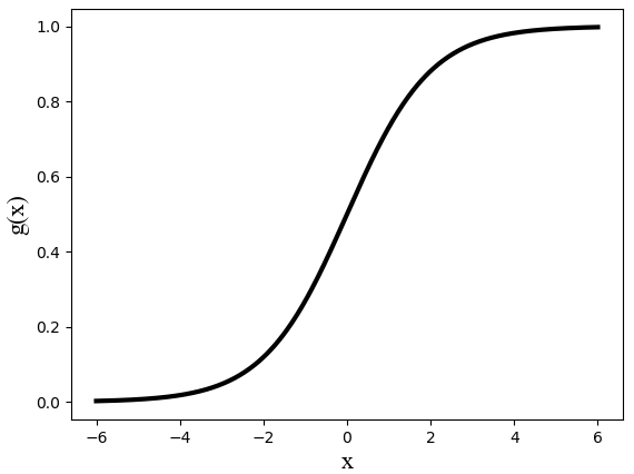
Intuitively, if we can formulate the quantization operation as a simple non-linear function similar to the common activation functions (e.g., Sigmoid sigmoid, ReLU relu or Maxout maxout), no approximation of gradients would be needed, and the quantization of any learnable parameters in DNNs, including activations and weights, can be learned straightforwardly and efficiently. Inspired by that, we present a novel perspective for interpreting and implementing quantization in neural networks. Specifically, we formulate quantization as a differentiable non-linear mapping function, termed quantization function. As shown in Fig. 1, the quantization function is formed as a linear combination of several Sigmoid functions with learnable biases and scales. In this way, the proposed quantization function can be learned in a lossless and end-to-end manner and works for any weights and activations in neural networks, avoiding the gradient mismatch problem. As illustrated in Fig. 2, the quantization is achieved via the continuous relaxation of the steepness of the Sigmoid functions during the training stage.
Our main contributions are summarized as follows:
- •
In contrast to existing low-bit quantization methods, we are the first to formulate quantization as a differentiable non-linear mapping function, which provides a simple/straightforward and general/uniform solution for any-bit weight and activation quantization, without suffering the severe gradient mismatch problem.
- •
We implement a simple and effective form of quantization networks, which could be learned in a lossless and end-to-end manner and outperform state-of-the-art quantization methods on both image classification and object detection tasks.
2 Related Work
In this paper, we propose formulating the quantization operation as a differentiable non-linear function. In this section, we give a brief review of both low-bit quantization methods and non-linear functions used in neural networks.
2.1 Low-Bit Quantization of Neural Networks
Approaches for quantizing full-precision networks into low-bit networks can be roughly divided into two categories: approximation-based and optimization-based. The first approach is to approximate the 32-bit full-precision values with discrete low-bit values in the forward pass of networks. BinaryConnect BinaryConnect directly optimizes the loss of the network with weights replaced by sign(), and approximates the sign function with the “hard tanh” function in the backward process, to avoid the zero-gradient problem. Binary weight network (BWN) xnor-net adds scale factors for the weights during binarization. Ternary weight network (TWN) twn introduces ternary weights and achieves better performance. Trained ternary quantization (TTQ) TTQ proposes learning both ternary values and scaled gradients for -bit weights. DoReFa-Net DoReFa proposes quantizing -bit weights, activations and gradients using different widths of bits. Gradients are approximated by a custom-defined form based on the mean of the absolute values of full-precision weights. In integer-net, weights, activations, gradients and errors are all approximated by low-bitwidth integers based on rounding and shifting operations. Jacob et al. integer-arithmetic propose an affine mapping of integers to real numbers that allows inference to be performed using integer-only arithmetic. As discussed before, the approximation-based methods use different forward and backward approximations, which causes a gradient mismatch problem. Friesen and Domingos iclr18 observe that setting targets for hard-threshold hidden units to minimize loss is a discrete optimization problem. Zhuang et al. telcnn propose a two-stage approach to quantize the weights and activations in a two-step manner. Lin et al. abcnet approximate full-precision weights with the linear combination of multiple binary weight bases. Zhang et al. lqnet propose an flexible un-uniform quantization method to quantize both network weights and activations. Cai et al. HWGQ used several piece-wise backward approximators to overcome the problem of gradient mismatch. Zhou et al. INQ proposed a decoupling step-by-step operation to efficiently convert a pre-trained full-precision convolutional neural network (CNN) model into a low-precision version. As a specific quantization, HashNet HashNet adopts a similar continuous relaxation to train the hash function, where a single tanh function is used for binarization. However, our training case (multi-bits quantization of both activations and weights in multi-layers) is much more complicated and challenging.
To avoid the gradient approximation problem, optimization-based quantization methods are recently proposed. They directly formulate the quantization of neural networks as a discretely constrained optimization problem admm; loss-aware. Leng et al. admm introduce convex linear constraints for the weights and solve the problem by the alternating direction method of multipliers (ADMM). Hou and Kwok loss-aware directly optimize the loss function w.r.t. the ternarized weights using proximal Newton algorithm. However, these methods are only suitable for quantization of weights and such iterative solution suffers from high computational costs in training.


2.2 Non-Linear Functions in Deep Neural Networks
In neural networks, the design of hidden units is distinguished by the choice of the non-linear activation function for hidden units deep-learning-book. The simplest form of a neural network is perceptron perceptron, where a unit step function is introduced to produce a binary output:
| (1) |
This form is similar to the binary quantization operation, i.e., discretize the continuous inputs into binary values. However, the problem is that it is not immediately obvious how to learn the perceptron networks NNDL-book.
To solve this problem, the sigmoid activation function is adopted in the early form of feedforward neural networks:
| (2) |
which has smooth and non-zero gradient everywhere so that the sigmoid neurons can be learned via back-propagation. When the absolute value of is very large, the outputs of a sigmoid function is close to a unit step function.
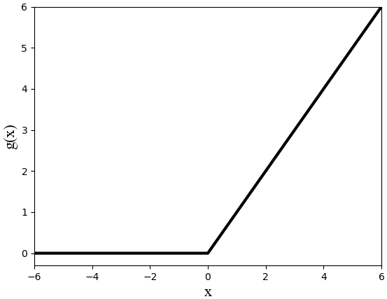
Currently, rectified linear units (ReLU) are more frequently used as the activation functions in deep neural networks:
| (3) |
The ReLU function outputs zero across half of its domain and is linear in the other half, which makes the DNNs easy to optimize.
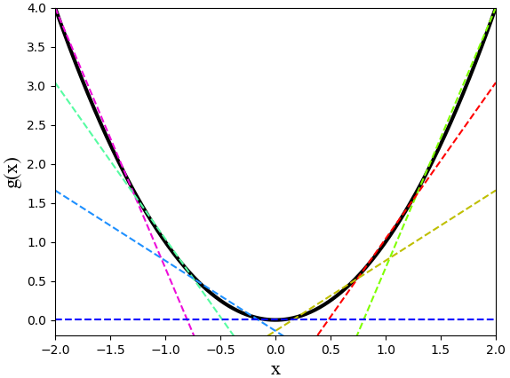
A generalization of the rectified linear units is Maxout. Its activation function is defined as:
| (4) |
where {} and {} are learned parameters. The form of Maxout indicates that a complex convex function can be approximated by a combination of simple linear functions.
3 Quantization Networks
The main idea of this work is to formulate the quantization operation as a differentiable non-linear function, which can be applied to any weights and activations in deep neural networks. We first present our novel interpretation of quantization from the perspective of non-linear functions. Then, our simple and effective quantization function is introduced and the learning of quantization networks are given.
3.1 Reformulation of Quantization
The quantization operation is mapping continuous inputs into discrete integer numbers, which is similar to the perceptron. Thus, from the perspective of non-linear mapping functions, a binary quantization operation can be formed of a unit step function. Inspired by the design of Maxout units, quantizing continuous values into a set of integer numbers can be formulated as a combination of several binary quantizations. In other words, the ideal low-bit quantization function is a combination of several unit step functions with specified biases and scales, as shown in Fig. 2(e):
| (5) |
where is the full-precision weight/activation to be quantized, is the quantized integer constrained to a predefined set , and is the number of quantization intervals. is the scale factor of inputs. is the standard unit step function. and are the scales and biases for the unit step functions, . The global offset keeps the quantized output zero-centered. Once the expected quantized integer set is given, , and offset can be directly obtained.
3.2 Training and Inference with Quantization Networks
Inspired by the advantage of sigmoid units against the perceptron in feedforward networks, we propose replacing the unit step functions in the ideal quantization function Eq. (5) with sigmoid functions. With this replacement, we can have a differentiable quantization function, termed soft quantization function, as shown in Fig. 2(c). Thus, we can learn any low-bit quantized neural networks in an end-to-end manner based on back propagation.
However, the ideal quantization function Eq. (5) is applied in the inference stage. The use of different quantization functions in training and inference stages may decrease the performance of DNNs. To narrow the gap between the ideal quantization function used in inference stage and the soft quantization function used in training stage, we introduce a temperature to the sigmoid function, motivated by the temperature introduced in distilling distilling,
| (6) |
With a larger , the gap between two quantization functions is smaller, but the learning capacity of the quantization networks is lower since the gradients of the soft quantization function will be zero in more cases. To solve this problem, in the training stage we start with a small to ensure the quantized networks can be well learned, and then gradually increase w.r.t. the training epochs. In this way, the quantized networks can be well learned and the gap between two quantization functions will be very small at the end of the training.
Forward Propagation. In detail, for a set of full-precision weights or activations to be quantized , the quantization function is applied to each independently:
| (7) |
where and are the scale factors of the input and output respectively. , where indicates the beginning of the input for the -th quantization interval except the first quantization interval, and the beginning of the first quantization interval is . The temperature controls the gap between the ideal quantization function and the soft quantization function. The gradual change from no quantization to complete quantization along with the adjustment of is depicted in Fig. 2.
The quantization function Eq. (7) is applied to every full-precision value that need to be quantized, just as applying ReLU in traditional DNNs. can be either a weight or an activation in DNNs. The output replaces for further computing.
Backward Propagation. During training stage, we need to back propagate the gradients of loss through the quantization function, as well as compute the gradients with respect to the involved parameters :
| (8) | ||||
| (9) | ||||
| (10) | ||||
| (11) |
where . we do not need to compute the gradients of , and offset , because their are directly obtained by . Our soft quantization function is a differentiable transformation that introduces quantized weights and activations into the network.
| 1/32 | 2/32 | 3(2)/32 | 3(4)/32 | 1/1 | 1/2 | |
|---|---|---|---|---|---|---|
| BinaryConnect BinaryConnect | 35.4/61.0 | - | - | - | 27.9/50.42 | - |
| BWN xnor-net | 56.8/79.4 | - | - | - | 44.2/69.2 | - |
| DoReFa DoReFa | 53.9/76.3 | - | - | - | 39.5/- | 47.7/- |
| TWN twn | - | 54.5/76.8 | - | - | - | - |
| TTQ TTQ | - | 57.5/79.7 | - | - | - | - |
| ADMM admm | 57.0/79.7 | 58.2/80.6 | 59.2/81.8 | 60.0/82.2 | - | - |
| HWGQ HWGQ | - | - | - | - | - | 52.7/76.3 |
| TBN TBN | - | - | - | - | - | 49.7/74.2 |
| LQ-Net lqnet | - | 60.5/82.7 | - | - | - | 55.7/78.8 |
| Ours | 58.8/81.7 | 60.9/83.2 | 61.5/83.5 | 61.9/83.6 | 47.9/72.5 | 55.4/78.8 |
Training and Inference. To quantize a network, we specify a set of weights or activations and insert the quantization function for each of them, according to Eq. (7). Any layer that previously received as an input, now receives . Any module that previously used as parameters, now uses . The smooth quantization function allows efficient training for networks, but it is neither necessary nor desirable during inference; we want the specified weights or activations to be discrete numbers. For this, once the network has been trained, we replace the sigmoid function in Eq. (7) by the unit step function for quantization:
| (12) |
Algorithm 1 summarizes the procedure for training quantization networks. For a full-precision network with modules, where a module can be either a convolutional layer or a fully connected layer, we denote all the activations to be quantized in the -th module as , and denote all the weights to be quantized in the -th module as . All elements in share the same quantization function parameters . All elements in share the same quantization function parameters . We apply the quantization function module by module. Then, we train the network with gradually increased temperature .
4 Experiments
4.1 Image Classification
To compare with state-of-the-art methods, we evaluate our method on ImageNet (ILSVRC 2012). ImageNet has approximately million training images from thousand categories and thousand validation images. We evaluate our method on AlexNet alexnet (over-parameterized architectures) and ResNet-18/ResNet-50 ResNet (compact-parameterized architectures). We report our classification performance using Top-1 and Top-5 accuracies with networks quantized to Binary({0, 1}, 1 bit), Ternary({-1, 0, 1}, 2 bits), {-2, -1, 0, 1, 2} (denoted as 3 bits(2)), {-4, -2, -1, 0, 1, 2, 4 } (denoted as 3 bits(4)), and {-15, -14, , -1, 0, 1, , 14, 15 } (5 bits). All the parameters are fine-tuned from pretrained full-precision models.
All the images from ImageNet are resized to have pixels for the smaller dimension, and then a random crop of is selected for training. Each pixel of the input images is subtracted by the mean values and divided by variances. Random horizontal flipping is introduced for preprocessing. No other data augmentation tricks are used in the learning process. The batch size is set to . Following xnor-net and twn, the parameters of the first convolutional layer and the last fully connected layer for classification are not quantized. For testing, images are resized to for the smaller side, and a center crop of is selected.
For our quantization function Eq. (7), to ensure all the input full-precision values lie in the linear region of our quantization function, the input scale is initialized as , where is the max absolute value of elements in and is the max absolute value of elements in . The output scale is initialized by , keeping the magnitude of the inputs unchanged after quantization.
Weight quantization: For binary quantization, only sigmoid function is needed; thus , , , and . For ternary quantization (), , and , ensuring that of the values in are quantized to as in twn. For the quantization of other bits, we first group the full-precision inputs into clusters by -means clustering. Then, the centers of the clusters are ranked in ascending order, and we get . For bias initialization, . Again, we set and to ensure that of the values in are quantized to .
| 1/32 | 2/32 | 3(2)/32 | 3(4)/32 | 5/32 | 1/1 | 1/2 | 32/2 | |
|---|---|---|---|---|---|---|---|---|
| BWN xnor-net | 60.8/83.0 | - | - | - | - | 51.2/73.2 | - | - |
| TWN twn | - | 61.8/84.2 | - | - | - | - | - | - |
| TTQ TTQ | - | 66.6/87.2 | - | - | - | - | - | - |
| INQ INQ | - | 66.0/87.1 | - | 68.1/88.4 | 69.0/89.1 | - | - | - |
| ABC-Net abcnet | - | - | - | - | 68.3/87.9 | 42.7/67.6 | - | - |
| HWGQ HWGQ | - | - | - | - | - | - | 59.6/82.2 | - |
| ADMM admm | 64.8/86.2 | 67.0/87.5 | 67.5/87.9 | 68.0/88.3 | - | - | - | - |
| ICLR18 iclr18 | - | - | - | - | - | - | - | 64.3/- |
| TBN TBN | - | - | - | - | - | - | 55.6/79.0 | - |
| LQ-Net lqnet | - | 68.0/88.0 | - | 69.3/88.8 | - | - | 62.6/84.3 | - |
| Ours | 66.5/87.3 | 69.1/88.9 | 69.9/89.3 | 70.4/89.6 | 70.6/89.6 | 53.6/75.3 | 63.4/84.9 | 65.7/86.5 |
| 1/32 | 2/32 | 3(2)/32 | 3(4)/32 | 5/32 | |
|---|---|---|---|---|---|
| BWN xnor-net | 68.7/- | - | - | - | - |
| TWN twn | - | 72.5/- | - | - | - |
| INQ INQ | - | - | - | - | 74.8/- |
| LQ-Net lqnet | - | 75.1/92.3 | - | - | - |
| Ours | 72.8/91.3 | 75.2/92.6 | 75.5/92.8 | 76.2/93.2 | 76.4/93.2 |
Activation quantization: Outputs of the ReLU units are used for activation quantization. It means that the block is Conv−-BN−-ReLU(-−Pooling)-−Quant in our method. The in Eq. (7) is set to because all activations are non-negative. For binary quantization(), only sigmoid function is needed, i.e. and . For two-bit quantization of activations (), and . is obtained by clustering as in weight quantization. We randomly sample 1000 samples from the dataset, and get the min/max activation values of the output layer by layer for ’s initialization .
The whole training process consists of phases. First, disable activation quantization and only train the quantization of weights. Second, fix the quantization of weights and only train the quantization of activations. Third, release quantization of both weights and activations until the model converges.
AlexNet: This network has five convolutional layers and two fully connected layers. This network is the mostly used benchmark for the quantization of neural networks. As in xnor-net; twn; admm, we use AlexNet coupled with batch normalization bn layers. We update the model by stochastic gradient descent (SGD) with the momentum set to . The learning rate is initialized by and decayed by at epochs and respectively. The model is trained for at most epochs in total. The weight decay is set to . The temperature is set to and increased linearly w.r.t. the training epochs, i.e., . Gradients are clipped with a maximum L2 norm of .
The results of different quantization methods are shown in Table 1. denotes both weights and activations are binary quantized. As shown, our quantization network outperforms state-of-the-art methods in both weight quantization and activation quantization. Moreover, our quantization network is highly flexible. It is suitable for arbitrary bits quantizaion and can be applied for quantization of both weights and activation.
ResNet: The most common baseline architectures, including AlexNet, VGG and GoogleNet, are all over-parameterized by design for accuracy improvements. Therefore, it is easy to obtain sizable compression of these architectures with a small accuracy degradation. A more meaningful benchmark would be to quantize model architectures that are already with efficient parameters, e.g., ResNet. We use the ResNet-18 and ResNet-50 proposed in ResNet.
The learning rate is decayed by at epochs and , and the model is trained for at most epochs in total. The weight decay is set to . The temperature is set to and increased linearly w.r.t the training epochs (). The other settings are the same as these for AlexNet. The results of different quantization methods are shown in Table 2 and Table 3 for ResNet-18 and ResNet-50, respectively. We can see that the performance degradation of quantized models is larger than that on AlexNet. This is reasonable because that the parameters of the original model are more compact. It’s worth noting that even in such a compact model, our method still achieves lossless results with only bits. And as far as we know, we are the first to surpass the full-precision model on ResNet-18 with bits weight quantization.


4.2 Object Detection
In order to evaluate our quantization network on object detection task, we test it on the popular architecture SSD (single shot multibox detection) ssd. The models are trained on Pascal VOC and train datasets, and are tested on Pascal VOC test dataset. We follow the same settings in ssd and the input images are resized to . Except the final convolutional layers with kernels and the first convolution layer, parameters of all other layers in the backbone VGG16 are quantized.
We update the model by SGD with the momentum set to . The initial learning rate is set to for quantized parameters, for non-quantized parameters and decayed by at epochs and . Models are trained for epochs in total. The batch size is set to and the weight decay is . We increase the temperature by every epoch, i.e., . Gradients are clipped with maximum L2 norm of .
The results are given in Table 4. Here we compare our model with ADMM only because other baseline quantization methods did not report their performance on object detection task. As shown in Table 4, our model is slightly better than ADMM. This result is very promising since our method is much simpler and much more general than ADMM.
| 2/32 | 3(4)/32 | 3(4)/8 | |
|---|---|---|---|
| ADMM admm | 76.2 | 77.6 | - |
| Ours | 76.3 | 77.7 | 76.1 |
4.3 Ablation Experiments
In this section we discuss about the settings of our quantization network. All statistics are collected from the training process of Alexnet and ResNet-18 on ImageNet.
Configuration of Bias . Generally, the quantized values are pre-defined linearly (e.g., ) or logarithmically (e.g., ) with a scale factor twn; integer-net; admm; DoReFa; loss-aware; integer-arithmetic. In this paper, we find that the distribution of full-precision parameters of pre-trained model is roughly subjected to Gaussian distribution, as shown in Fig. 3. It indicates that quantizing weights into linear or logarithmical intervals may not be the most suitable way. Thus, a non-uniform quantization (e.g. K-means clustering) is adopted to counterbalance this. So, we use the clustering centers to determine the boundaries of quantization intervals {}. The experimental results in Table 5 demonstrate the superior of non-uniform quantization over linear quantization. We also find that adaptive learning of biases during training does not show superiority over the fixed version. Therefore, we freeze the biases after initialization in all experiments.
| Quantization methods | W/A | Top-1 | Top-5 |
|---|---|---|---|
| linear | 2/32 | ||
| non-uniform | 2/32 | 60.9 | 83.2 |
| linear | 3(4)/32 | ||
| non-uniform | 3(4)/32 | 61.9 | 83.6 |
Effect of layer-wise quantization. As shown in Fig. 3, the parameter magnitudes are quite different from layer to layer (full-precision network). Therefore, it is unsuitable and less efficient to use a shared quantization function across layers. We adopt layer-wise quantization in this paper, i.e., weights/activations from the same layer share the same quantization function and weights/activations from different layers use different quantization functions. Table 6 shows a comparison between shared quantization function across layers and layer-wise shared quantization function.
| Quantization methods | W/A | Top-1 | Top-5 |
|---|---|---|---|
| shared | 2/32 | ||
| layer-wise | 2/32 | 60.9 | 83.2 |
Effect of Temperature. As discussed in Section 3, the temperature controls the gap between the hard quantization function Eq. (12) in the inference stage and the soft quantization function Eq. (7) in the training stage. In order to investigate the effect of this gap to the performance of quantized network, we compare the testing accuracy of the models (trained with different s) when soft and hard quantization functions are adopted, as shown in Fig. 4. We can see that as the temperature increases, the difference between them is gradually reduced. Thus, gradually increasing temperature during training can achieve a good balance between model learning capacity and quantization gap.


Training from pre-trained model. In our training, the temperature parameter is increased linearly w.r.t. the training epochs. When training from scratch, the temperature may become quite large before the network is well-converged, and the saturated neurons will slow down the network training process and make the network stuck in bad minima. According to Table 7, training from a pre-trained model could greatly improve the performance compared to training from scratch.
| Training methods | W/A | Top-1 | Top-5 |
|---|---|---|---|
| from scratch | 3(4)/32 | ||
| from pre-trained | 3(4)/32 | 70.4 | 89.6 |
Time-space complexity of the final model for inference. Table 8 shows the time-space complexities of the final quantization networks for inference based on VU9P FPGA evaluation. We can see that both time and space complexity are significantly reduced via low-bit quantization of Neural Networks.
| Binary | Ternary | Full-precision | |
|---|---|---|---|
| Time | 1x | 1.4x | 45x |
| Space | 1x | 2x | 32x |
Convergence for Temprature . The training process is very stable w.r.t. different s (shown in Fig. 5). The approximation of the final “soft” quantization function to a “hard” step function is determined by the final temperature, which is controlled by the maximum training epoch (). The increasing speed of temperature (e.g.10) controls the speed of convergence (or learning rate) from a “soft” to “hard” quantization (shown in Figure in our paper), and it is consistent with the learning progress of the backbone model. Practically, for differentbackbone models, we can tune in via performance on validation set as the way of learning rate for DL models.


5 Conclusion
This work focused on interpreting and implementing low-bit quantization of deep neural networks from the perspective of non-linear functions. Inspired by activation functions in DNNs, a soft quantization function is proposed and incorporated in deep neural networks as a new kind of activation function. With this differentiable non-linear quantization function embedded, quantization networks can be learned in an end-to-end manner. Our quantization method is highly flexible. It is suitable for arbitrary bits quantization and can be applied for quantization of both weights and activations. Extensive experiments on image classification and object detection tasks have verified the effectiveness of the proposed method.
Acknowledgements
This work was supported in part by the National Key R&D Program of China under contract No. 2017YFB1002203 and NSFC No. 61872329.
References
- (1) Zhaowei Cai, Xiaodong He, Jian Sun, and Nuno Vasconcelos. Deep learning with low precision by half-wave gaussian quantization. In CVPR, pages 5406–5414, 2017.
- (2) Zhangjie Cao, Mingsheng Long, Jianmin Wang, and S Yu Philip. Hashnet: Deep learning to hash by continuation. In ICCV, pages 5609–5618, 2017.
- (3) Wenlin Chen, James Wilson, Stephen Tyree, Kilian Weinberger, and Yixin Chen. Compressing neural networks with the hashing trick. In ICML, pages 2285–2294, 2015.
- (4) Matthieu Courbariaux, Yoshua Bengio, and Jean-Pierre David. Binaryconnect: Training deep neural networks with binary weights during propagations. In NIPS, pages 3123–3131, 2015.
- (5) Abram L Friesen and Pedro Domingos. Deep learning as a mixed convex-combinatorial optimization problem. arXiv preprint arXiv:1710.11573, 2017.
- (6) Ian J. Goodfellow, David Warde-Farley, Mehdi Mirza, Aaron C. Courville, and Yoshua Bengio. Maxout networks. In ICML, pages 1319–1327, 2013.
- (7) Song Han, Jeff Pool, John Tran, and William J. Dally. Learning both weights and connections for efficient neural networks. In NIPS, pages 1135–1143, 2015.
- (8) Kaiming He, Xiangyu Zhang, Shaoqing Ren, and Jian Sun. Deep residual learning for image recognition. In CVPR, pages 770–778, 2016.
- (9) Geoffrey Hinton, Oriol Vinyals, and Jeff Dean. Distilling the knowledge in a neural network. arXiv preprint arXiv:1503.02531, 2015.
- (10) Lu Hou and James T. Kwok. Loss-aware weight quantization of deep networks. In ICLR, 2018.
- (11) Andrew G Howard, Menglong Zhu, Bo Chen, Dmitry Kalenichenko, Weijun Wang, Tobias Weyand, Marco Andreetto, and Hartwig Adam. Mobilenets: Efficient convolutional neural networks for mobile vision applications. arXiv preprint arXiv:1704.04861, 2017.
- (12) Yoshua Bengio Ian Goodfellow and Aaron Courville. Deep learning. Book in preparation for MIT Press, 2016.
- (13) Forrest N Iandola, Song Han, Matthew W Moskewicz, Khalid Ashraf, William J Dally, and Kurt Keutzer. Squeezenet: Alexnet-level accuracy with 50x fewer parameters and¡ 0.5 mb model size. arXiv preprint arXiv:1602.07360, 2016.
- (14) Sergey Ioffe and Christian Szegedy. Batch normalization: Accelerating deep network training by reducing internal covariate shift. In ICML, pages 448–456, 2015.
- (15) Benoit Jacob, Skirmantas Kligys, Bo Chen, Menglong Zhu, Matthew Tang, Andrew G. Howard, Hartwig Adam, and Dmitry Kalenichenko. Quantization and training of neural networks for efficient integer-arithmetic-only inference. In CVPR, pages 2704–2713, 2018.
- (16) Max Jaderberg, Andrea Vedaldi, and Andrew Zisserman. Speeding up convolutional neural networks with low rank expansions. In BMVC, 2014.
- (17) Joe Kilian and Hava T Siegelmann. On the power of sigmoid neural networks. In COLT, pages 137–143, 1993.
- (18) Alex Krizhevsky, Ilya Sutskever, and Geoffrey E. Hinton. Imagenet classification with deep convolutional neural networks. In NIPS, pages 1106–1114, 2012.
- (19) Abhisek Kundu, Kunal Banerjee, Naveen Mellempudi, Dheevatsa Mudigere, Dipankar Das, Bharat Kaul, and Pradeep Dubey. Ternary residual networks. arXiv preprint arXiv:1707.04679, 2017.
- (20) Cong Leng, Hao Li, Shenghuo Zhu, and Rong Jin. Extremely low bit neural network: Squeeze the last bit out with admm. In AAAI, pages 3466–3473, 2018.
- (21) Fengfu Li and Bin Liu. Ternary weight networks. arXiv preprint arXiv:1605.04711v2, 2016.
- (22) Zefan Li, Bingbing Ni, Wenjun Zhang, Xiaokang Yang, and Wen Gao. Performance guaranteed network acceleration via high-order residual quantization. In ICCV, pages 2603–2611, 2017.
- (23) Xiaofan Lin, Cong Zhao, and Wei Pan. Towards accurate binary convolutional neural network. In NIPS, pages 345–353, 2017.
- (24) Wei Liu, Dragomir Anguelov, Dumitru Erhan, Christian Szegedy, Scott E. Reed, Cheng-Yang Fu, and Alexander C. Berg. Ssd: Single shot multibox detector. In ECCV, pages 21–37, 2016.
- (25) Vinod Nair and Geoffrey E. Hinton. Rectified linear units improve restricted boltzmann machines. In ICML, pages 807–814, 2010.
- (26) Michael A. Nielsen. Neural networks and deep learning. Determination Press, 2015.
- (27) Mohammad Rastegari, Vicente Ordonez, Joseph Redmon, and Ali Farhadi. Xnor-net: Imagenet classification using binary convolutional neural networks. In ECCV, pages 525–542, 2016.
- (28) Frank Rosenblatt. The perceptron: A probabilistic model for information storage and organization in the brain. Psychological Review, pages 65–386, 1958.
- (29) Diwen Wan, Fumin Shen, Li Liu, Fan Zhu, Jie Qin, Ling Shao, and Heng Tao Shen. Tbn: Convolutional neural network with ternary inputs and binary weights. In ECCV, pages 315–332, 2018.
- (30) Shuang Wu, Guoqi Li, Feng Chen, and Luping Shi. Training and inference with integers in deep neural networks. In ICLR, 2018.
- (31) Dongqing Zhang, Jiaolong Yang, Dongqiangzi Ye, and Gang Hua. Lq-nets: Learned quantization for highly accurate and compact deep neural networks. In ECCV, pages 365–382, 2018.
- (32) Aojun Zhou, Anbang Yao, Yiwen Guo, Lin Xu, and Yurong Chen. Incremental network quantization: Towards lossless cnns with low-precision weights. In ICLR, 2017.
- (33) Shuchang Zhou, Yuxin Wu, Zekun Ni, Xinyu Zhou, He Wen, and Yuheng Zou. Dorefa-net: Training low bitwidth convolutional neural networks with low bitwidth gradients. arXiv preprint arXiv:1606.06160, 2016.
- (34) Chenzhuo Zhu, Song Han, Huizi Mao, and William J. Dally. Trained ternary quantization. In ICLR, 2017.
- (35) Bohan Zhuang, Chunhua Shen, Mingkui Tan, Lingqiao Liu, and Ian Reid. Towards effective low-bitwidth convolutional neural networks. In CVPR, pages 7920–7928, 2018.