The asymptotics of the clustering transition for random constraint satisfaction problems

As mentioned in the introduction the dynamic transition $\alpha_{\rm d}$ can be characterized in several ways; we shall exploit here the perspective provided by the tree reconstruction problem, that we now briefly describe in the specific case of the hypergraph bicoloring, referring the reader to MoPe03; MezardMontanari06 for more generic and extensive discussions. Consider an hypertree $G=(V,E)$, with vertices $i\in V$, and hyperedges $a\in E$, where an hyperedge is a set denoted $\partial a$ of $k\geq 3$ vertices (see Fig. 1 for an example); we shall denote similarly $\partial i$ the set of hyperedges adjacent to a vertex $i$. An Ising spin variable $\sigma_{i}\in\{-1,+1\}$ is placed on each vertex $i\in V$ of the hypertree, with their global configuration denoted $\underline{\sigma}=\{\sigma_{i},i\in V\}$, the notation $\underline{\sigma}_{S}=\{\sigma_{i},i\in S\}$ corresponding to the configuration on a subset $S\subset V$ of the vertices. A proper bicoloring of $G$ is defined as a configuration $\underline{\sigma}$ such that no hyperedge is monochromatic, in other words every hyperedge must have among its $k$ neighboring vertices at least one spin equal to $+1$ and one equal to $-1$. The uniform distribution over these proper bicolorings, $\eta(\underline{\sigma})$, can thus be written as

$$\eta(\underline{\sigma})=\frac{1}{Z}\prod_{a\in E}w(\underline{\sigma}_{\partial a})\ ,\qquad w(\sigma_{1},\dots,\sigma_{k})=\mathbb{I}(\sigma_{1},\dots,\sigma_{k}\,\text{n.a.e.})=1-\mathbb{I}(\sigma_{1}=\dots=\sigma_{k})\ ,$$

(2)

where $Z$ is a normalizing factor counting the number of proper bicolorings, $\mathbb{I}(A)$ is the indicator function of the event $A$, and n.a.e. is the abbreviation of not all equal.

Thanks to the invariance of $\eta$ under a global spin flip, $\eta(-\underline{\sigma})=\eta(\underline{\sigma})$, and to the acyclic property of the tree $G$, it is actually easy to sample configurations from $\eta$ by a recursive, broadcasting procedure described as follows. Choose an arbitrary vertex $i_{0}$ to be called the root of the tree (the one drawn at the top of Fig. 1), and set its spin $\sigma_{i_{0}}$ to $\pm 1$ with probability $1/2$. Then, independently for each edge $a$ adjacent to the root, draw the configuration of the $k-1$ other variables with the conditional probability $p(\underline{\sigma}_{\partial a\setminus i_{0}}|\sigma_{i_{0}})$, where

$$p(\sigma_{1},\dots,\sigma_{k-1}|\sigma)=\frac{1}{2^{k-1}-1}(1-\mathbb{I}(\sigma_{1}=\dots=\sigma_{k-1}=\sigma))\ .$$

(3)

Once the values of all the spins at distance 1 from the root have been set in this way the same process can be iterated, each of these vertices of the first generation being in turn considered as the root of the subtree lying below it.

This description of the sampling from $\eta$ as a broadcast process naturally calls for an interpretation as the transmission of an information, the value of the spin at the root, through noisy channels, the hyperedges, towards a set of receivers, the vertices at a certain distance $n$ from the root, to be denoted $B_{n}$. In this information theoretic perspective the tree reconstruction problem asks the following question: given only the values $\underline{\sigma}_{B_{n}}$ of the spins at distance $n$ from the root in a configuration $\underline{\sigma}$ generated as above, how much information is available on the value of the root $\sigma_{i_{0}}$, and does a non-vanishing amount of information on $\sigma_{i_{0}}$ survives in the $n\to\infty$ limit ? This question is equivalent to the existence of long-range non-trivial point-to-set correlations under the probability measure $\eta$, the “point” being the root and the “set” the vertices at distance $n$ from it. In this Bayesian setting the information-theoretical optimal strategy of an observer having to reconstruct $\sigma_{i_{0}}$ from $\underline{\sigma}_{B_{n}}$ is to compute the posterior probability $\eta(\sigma_{i_{0}}|\underline{\sigma}_{B_{n}})$. Thanks to the tree structure of the interaction graph this strategy is actually computationally feasible and can be performed in a recursive way. Consider indeed the so-called Belief Propagation (BP) equations, also known as message passing or dynamic programming algorithm KschischangFrey01, bearing upon probability measures over $\{-1,+1\}$, $\eta_{i\to a}$, $\widehat{\eta}_{a\to i}$ for each edge between an hyperedge $a$ and an adjacent vertex $i\in\partial a$:

$$\eta_{i\to a}(\tau_{i})=\frac{1}{z_{i\to a}}\prod_{b\in\partial i\setminus a}\widehat{\eta}_{b\to i}(\tau_{i})\ ,\quad\widehat{\eta}_{a\to i}(\tau_{i})=\frac{1}{z_{a\to i}}\sum_{\underline{\tau}_{\partial a\setminus i}}w(\tau_{i},\underline{\tau}_{\partial a\setminus i})\prod_{j\in\partial a\setminus i}\eta_{j\to a}(\tau_{j})\ ,$$

(4)

where $z_{i\to a}$ and $z_{a\to i}$ are chosen to enforce the normalization of these probability laws. A moment of thought reveals that, once supplemented by the boundary conditions

$$\eta_{i\to a}(\tau_{i})=\delta_{\tau_{i},\sigma_{i}}\ \ \text{for}\ \ i\in B_{n}\ ,$$

(5)

these BP equations admit a unique solution for any finite tree, and that the posterior probabilities $\eta(\sigma_{i}|\underline{\sigma}_{B_{n}})$ can be determined, for $i\notin B_{n}$, from these messages according to

$$\eta(\sigma_{i}|\underline{\sigma}_{B_{n}})=\frac{1}{z_{i}}\prod_{a\in\partial i}\widehat{\eta}_{a\to i}(\sigma_{i})\ ,$$

(6)

with again $z_{i}$ a normalizing constant; note that in order to lighten the notations we have kept implicit the dependency of the messages on the observed variables $\underline{\sigma}_{B_{n}}$. As the messages $\eta_{i\to a}$ and $\widehat{\eta}_{a\to i}$ are probability distributions over a binary variable they can be parametrized by a single real number, that we shall denote $h_{i\to a}$ and $u_{a\to i}$ respectively, and define by

$$\eta_{i\to a}(\tau_{i})=\frac{1+h_{i\to a}\tau_{i}}{2}\ ,\qquad\widehat{\eta}_{a\to i}(\tau_{i})=\frac{1+u_{a\to i}\tau_{i}}{2}\ .$$

(7)

These numbers $h_{i\to a}$ and $u_{a\to i}$ are the average values of $\tau_{i}$ under the laws $\eta_{i\to a}$ and $\widehat{\eta}_{a\to i}$, they are thus in $[-1,1]$ and correspond to the magnetization of the spin; with a slight abuse of vocabulary we shall sometimes call them “fields” in the following. With this parametrization, and for the special case of the hypergraph bicoloring problem, the BP equations (4) become

$$h_{i\to a}=f(\{u_{b\to i}\}_{b\in\partial i\setminus a})\ ,\qquad u_{a\to i}=g(\{h_{j\to a}\}_{j\in\partial a\setminus i})\ ,$$

(8)

with the functions $f$ and $g$ defined by

$$f(u_{1},\dots,u_{l})=\frac{\underset{i=1}{\overset{l}{\prod}}\frac{1+u_{i}}{2}-\underset{i=1}{\overset{l}{\prod}}\frac{1-u_{i}}{2}}{\underset{i=1}{\overset{l}{\prod}}\frac{1+u_{i}}{2}+\underset{i=1}{\overset{l}{\prod}}\frac{1-u_{i}}{2}}\ ,\qquad g(h_{1},\dots,h_{k-1})=\frac{\underset{i=1}{\overset{k-1}{\prod}}\frac{1-h_{i}}{2}-\underset{i=1}{\overset{k-1}{\prod}}\frac{1+h_{i}}{2}}{2-\underset{i=1}{\overset{k-1}{\prod}}\frac{1+h_{i}}{2}-\underset{i=1}{\overset{k-1}{\prod}}\frac{1-h_{i}}{2}}\ .$$

(9)

The boundary condition (5) becomes

$$h_{i\to a}=\sigma_{i}\ \ \text{for}\ \ i\in B_{n}\ ,$$

(10)

and the average value of the spin at the root, in the posterior probability measure conditional on the observations of the spins at distance $n$, reads

$$h_{i_{0}}=\sum_{\sigma_{i_{0}}}\sigma_{i_{0}}\eta(\sigma_{i_{0}}|\underline{\sigma}_{B_{n}})=f(\{u_{a\to i_{0}}\}_{a\in\partial i_{0}})\ .$$

(11)

It is this value which has to be compared with the actual value of $\sigma_{i_{0}}$ in the broadcast process that led to $\underline{\sigma}_{B_{n}}$ in order to assess the amount of information transmitted between $i_{0}$ and $B_{n}$; once averaged over $\eta(\underline{\sigma})$ this yields the point-to-set correlation function.

The computation descrived above was performed for a given tree. Suppose now that the tree itself is random, and drawn as an instance of a Galton-Watson process with $n$ generations, in which every vertex has a random offspring (number of descendent hyperedges) distributed as a Poisson law of parameter denoted $\alpha k$. Let us call as above $h\in[-1,1]$ the posterior magnetization of the root given the observations of the spins on the vertices of the $n$-th generation (the root corresponding to the generation $n=0$). $h$ is a random variable because of the randomness in the generation of the Galton-Watson tree on the one hand, and in the broadcast process yielding $\underline{\sigma}_{B_{n}}$ on the other hand. We shall denote $P_{\sigma,n}(h)$ its distribution when the broadcast is conditioned to the root being equal to $\sigma$. As both the broadcast process (from the root downwards) and the resolution of the BP equations (from the leaves upwards) decompose recursively along the branches of the tree, it is possible to obtain from the above analysis an inductive formula relating these distributions for trees of depth $n$ and $n+1$, namely

	$\displaystyle P_{\sigma,n+1}(h)$	$\displaystyle=\sum_{l=0}^{\infty}e^{-\alpha k}\frac{(\alpha k)^{l}}{l!}\int\prod_{i=1}^{l}{\rm d}\widehat{P}_{\sigma,n}(u_{i})\,\delta(h-f(u_{1},\dots,u_{l}))\ ,$		(12)
	$\displaystyle\widehat{P}_{\sigma,n}(u)$	$\displaystyle=\sum_{\sigma_{1},\dots,\sigma_{k-1}}p(\sigma_{1},\dots,\sigma_{k-1}|\sigma)\int\prod_{i=1}^{k-1}{\rm d}P_{\sigma_{i},n}(h_{i})\,\delta(u-g(h_{1},\dots,h_{k-1}))\ ,$		(13)

with the initial condition $P_{\sigma,0}(h)=\delta(h-\sigma)$ that expresses the observation of the variables at the boundary of the tree. These are examples of Recursive Distributional Equations (RDEs), as they define by recursion a sequence of probability distributions. They can be equivalently written as equalities in distribution between random variables, for instance (12) means $h\overset{\rm d}{=}f(u_{1},\dots,u_{l})$ with $h$ drawn from $P_{\sigma,n+1}$, $l$ is a Poisson distributed random variable with mean $\alpha k$, and the $u_{i}$’s are i.i.d. copies of a random variable of law $\widehat{P}_{\sigma,n}$.

One can slightly simplify these equations by noticing that the invariance of the bicoloring problem under a global spin-flip of all its variables implies that $P_{-\sigma,n}(h)=P_{\sigma,n}(-h)$ and $\widehat{P}_{-\sigma,n}(u)=\widehat{P}_{\sigma,n}(-u)$; this can be checked by induction from (12,13), using $p(\sigma_{1},\dots,\sigma_{k-1}|\sigma)=p(-\sigma_{1},\dots,-\sigma_{k-1}|-\sigma)$ and the fact that $f$ and $g$ change sign when all their arguments are multiplied by $-1$. It is thus redundant to track the evolution with $n$ of the distributions with both $\sigma=+1$ and $\sigma=-1$, we shall instead define $P_{n}(h)=P_{+1,n}(h)$ and $\widehat{P}_{n}(u)=\widehat{P}_{+1,n}(u)$ and close the equations on these two sequences of distributions:

	$\displaystyle P_{n+1}(h)$	$\displaystyle=\sum_{l=0}^{\infty}e^{-\alpha k}\frac{(\alpha k)^{l}}{l!}\int\prod_{i=1}^{l}{\rm d}\widehat{P}_{n}(u_{i})\,\delta(h-f(u_{1},\dots,u_{l}))\ ,$		(14)
	$\displaystyle\widehat{P}_{n}(u)$	$\displaystyle=\sum_{\sigma_{1},\dots,\sigma_{k-1}}p(\sigma_{1},\dots,\sigma_{k-1}|+1)\int\prod_{i=1}^{k-1}{\rm d}P_{n}(h_{i})\,\delta(u-g(h_{1}\sigma_{1},\dots,h_{k-1}\sigma_{k-1}))\ .$		(15)

The answer to the reconstructibility question raised above can be read off from the behavior of $P_{n}(h)$ in the large $n$ limit: if it tends to the trivial distribution $\delta(h)$ (which is always a stationary solution of (14,15)), then all information on the value of the root has been washed out and the reconstruction problem is not solvable. On the contrary if the limit of $P_{n}(h)$ is non-trivial then the observation of $\underline{\sigma}_{B_{n}}$ contains some information on the root and the problem is said to be solvable. The occurence of these two situations depend on the parameters $k$ and $\alpha$ of the model; increasing $\alpha$ gives rise to a larger number of spin variables to be observed, which makes the inference problem easier. Hence it is natural to expect the existence of a threshold $\alpha_{\rm d}(k)$ such that the problem is unsolvable (resp. solvable) for $\alpha<\alpha_{\rm d}(k)$ (resp. $\alpha>\alpha_{\rm d}(k)$).

It is actually more convenient to describe this transition by a scalar order parameter (instead of the functional one $P_{n}$), the point-to-set correlation function that we shall define as

$$C_{n}(\alpha,k)=\int{\rm d}P_{n}(h)\,h\ ,\qquad C(\alpha,k)=\lim_{n\to\infty}C_{n}(\alpha,k)\ .$$

(16)

This is indeed an order parameter for the transition in the sense that $C(\alpha,k)>0$ if and only if $\alpha>\alpha_{\rm d}(k)$. This equivalence is a consequence of some symmetry properties of the distributions $P_{n}$ that we will describe now.

Let us call $T_{n}(h)$ the distribution of the posterior magnetization $h$ of the root, in a broadcast process which is not conditioned on the value of the root in $\underline{\sigma}$, i.e. $T_{n}(h)=(P_{+,n}(h)+P_{-,n}(h))/2$. A consequence of Bayes theorem applied to the joint law between the spins at the root and on the boundary vertices is the following converse relation between conditional and unconditional laws, $P_{\sigma,n}(h)=(1+\sigma h)T_{n}(h)$ (see MezardMontanari06; MoReTe11_recclus; RichardsonUrbanke07 for more details on this property and its consequences). In addition the invariance of the problem under a global spin-flip implies that $T_{n}(-h)=T_{n}(h)$, which yields a symmetry constraint on the distributions $P_{n}$,

$$P_{n}(-h)=\frac{1-h}{1+h}\,P_{n}(h)\ ,\qquad\int{\rm d}P_{n}(h)\,b(h)=\int{\rm d}P_{n}(h)\,b(-h)\,\frac{1-h}{1+h}\ ,$$

(17)

the second equality being valid for any function $b(h)$ such that the integrals exist. This symmetry (sometimes called Nishimori symmetry NishimoriBook01, and also fulfilled by $\widehat{P}_{n}(u)$) implies several identities between the moments of $h$ that can be derived by appropriate choices of the test function $b$ MoReTe11_recclus; RichardsonUrbanke07; here we shall only state the simplest one, namely

$$C_{n}(\alpha,k)=\int{\rm d}P_{n}(h)\,h=\int{\rm d}P_{n}(h)\,h^{2}\ ,$$

(18)

that can be obtained from (17) with $b(h)=h(1-h)$. This is enough to justify our statement of the characterization of the reconstruction transition via the behavior of $C_{n}$: if the latter vanishes in the $n\to\infty$ limit this implies that both the average and the variance of $P_{n}$ go to zero, hence $P_{n}$ tends to the trivial distribution $\delta(h)$.

The distributional equations (14,15) can be solved numerically relatively easily for finite values of $k$ by using a population dynamics algorithm ACTA73; MezardParisi01, whose main idea is to approximate a probability distribution by the empirical distribution of a large sample of representative elements. Suppose indeed that at some step $n$ one has an approximation of $P_{n}(h)$ written as

$\displaystyle P_{n}(h)\approx\frac{1}{{\cal N}}\sum_{i=1}^{\cal N}\delta(h-h_{i}^{(n)})\ ,$

(19)

where ${\cal N}\gg 1$ is the size of the population, that controls the numerical accuracy of the procedure. One can then insert this form in the r.h.s. of (15) to obtain an approximation of $\widehat{P}_{n}(u)$ as

$\displaystyle\widehat{P}_{n}(u)\approx\frac{1}{{\cal N}}\sum_{i=1}^{\cal N}\delta(u-u_{i}^{(n)})\ ,$

(20)

where each of the representants $u_{i}^{(n)}$ has been constructed independently by drawing $\sigma_{1},\dots,\sigma_{k-1}$ according to the law $p(\sigma_{1},\dots,\sigma_{k-1}|+)$, then $k-1$ indices $i_{1},\dots,i_{k-1}$ uniformly at random in $\{1,\dots,\cal N\}$, and setting $u_{i}^{(n)}=g\left(\sigma_{1}h_{i_{1}}^{(n)},\dots,\sigma_{k-1}h_{i_{k-1}}^{(n)}\right)$. Similarly, $P_{n+1}(h)$ can be approximated by an empirical distribution of the form (19), where according to (14) each of the representants $h_{i}^{(n+1)}$ is obtained by drawing an integer $l$ from the Poisson law $p_{l}=e^{-\alpha k}\frac{(\alpha k)^{l}}{l!}$, then $l$ indices $i_{1},\dots,i_{l}$ uniformly at random in $\{1,\dots,\cal N\}$, and taking $h_{i}^{(n+1)}=f\left(u_{i_{1}}^{(n)},\dots,u_{i_{l}}^{(n)}\right)$. The initial condition $P_{0}(h)=\delta(h-1)$ can obviously be represented by a sample with all representants $h_{i}^{(0)}$ equal to 1, and at every iteration step observables can be estimated as empirical averages,

$$\int{\rm d}P_{n}(h)F(h)\approx\frac{1}{{\cal N}}\sum_{i=1}^{\cal N}F(h_{i}^{(n)})$$

(21)

for an arbitrary function $F$.

The figure 2 presents some numerical results obtained with this procedure. The left panel displays the decay of the correlation function $C_{n}(\alpha,k)$ as a function of the distance $n$ for different values of $\alpha$ and $k=5$ (all values of $k$ large enough are qualitatively similar, but small values of $k$ behaves differently, see for instance gabrie2017phase). When $\alpha$ is small this function decays to 0 as $n\to\infty$, signalling the impossibility of reconstruction; when $\alpha$ increases the decay gets slower and proceeds in two steps, with a longer and longer plateau at a strictly positive value developping as $\alpha$ gets closer to the transition; finally for $\alpha>\alpha_{\rm d}$ the plateau lasts forever, the large $n$ limit $C(\alpha,k)$ is strictly positive. This quantity, that jumps discontinuously from 0 to a strictly positive value when $\alpha$ crosses $\alpha_{\rm d}$, is plotted as a function of $\alpha$ in the right panel of Fig. 2. To increase the numerical accuracy we estimated the limit by averaging the value of $C_{n}$ when $n$ is large enough to have reached its plateau behavior.

The definition of the reconstruction transition $\alpha_{\rm d}$ and its analysis in terms of the RDE on $P_{n}$ described above are based on the optimal inference algorithm, namely the computation of the posterior probability $\eta(\sigma_{i}|\underline{\sigma}_{B_{n}})$ via the BP equations (4). One can nevertheless consider a simpler, suboptimal inference procedure, that aims at answering the following question: is $\sigma_{i}$ uniquely determined in the measure $\eta(\cdot|\underline{\sigma}_{B_{n}})$, in other words is $\sigma_{i}$ constant in all the proper bicolorings of the graphs that take the values $\underline{\sigma}_{B_{n}}$ on the boundary vertices? It is clear that if the answer is yes then the inferred value of $\sigma_{i}$ is the correct one that was used in the broadcast, hence if reconstruction is possible in this strong sense of certain inference it is also possible in the definition introduced above.

We shall now determine the probability of success of this naive reconstruction procedure, that corresponds to a projection of the BP algorithm towards its Warning Propagation BraunsteinMezard05 version that only keeps sure beliefs and discards partially biased ones. To incorporate naturally this computation in the one presented above we decompose the field distributions as follows:

$$P_{n}(h)=w_{n}\,\delta(h-1)+(1-w_{n})\,Q_{n}(h)\ ,\qquad\widehat{P}_{n}(u)=\widehat{w}_{n}\,\delta(u-1)+(1-\widehat{w}_{n})\,\widehat{Q}_{n}(u)\ ,$$

(22)

where $Q_{n}$ and $\widehat{Q}_{n}$ are probability measures with no atom in $1$. The weight $w_{n}$ of the “hard field” $h=1$, that constrain completely the variable at the root and makes it a frozen variable under the boundary condition $\underline{\sigma}_{B_{n}}$, is precisely the probability of success of the naive reconstruction procedure. In the following we shall call $Q_{n}$ and $\widehat{Q}_{n}$ the distributions of soft fields; note that they do not contain atoms in $-1$ (because a variable $\sigma_{i}$ cannot be forced by $\underline{\sigma}_{B_{n}}$ to another value that it had in the broadcast), and that they enjoy the same Bayes symmetry (17) as the complete distributions $P_{n}$ and $\widehat{P}_{n}$. Inserting this decomposition in (14,15), and considering the possible combinations of arguments of the functions $f,g$ in (9) that yields $h,u=1$ one easily obtains the following evolution equations for $w_{n}$ and $\widehat{w}_{n}$:

$$w_{n+1}=1-e^{-\alpha k\widehat{w}_{n}}\ ,\qquad\widehat{w}_{n}=\frac{w_{n}^{k-1}}{2^{k-1}-1}\ .$$

(23)

The first one expresses the fact that a spin is perfectly recovered as soon as one of its neighboring interactions forces it to its correct value, while the second one shows that this latter event happens when in the broadcast the $k-1$ variables adjacent to it have been given the same value, and that they all have been perfectly recovered.

Assembling these two equations we obtain a simple recursive equation on $w_{n}$,

$$w_{n+1}=1-e^{-\Gamma(\alpha,k)w_{n}^{k-1}}\ ,\qquad\Gamma(\alpha,k)=\frac{\alpha k}{2^{k-1}-1}\ ,$$

(24)

with the initial condition $w_{0}=1$. By a numerical inspection of the shape of this recursion function one easily realizes that for $k\geq 3$ the fixed point reached by $w_{n}$ for $n\to\infty$ undergoes a discontinuous bifurcation from zero to a strictly positive value when $\Gamma$ crosses a critical value $\Gamma_{\rm r}=\Gamma_{\rm r}(k)$. The latter can be determined by noting that at such a bifurcation the derivative of the recursion function must be equal to 1, hence that $\Gamma_{\rm r}$ and $w_{\rm r}$, the fixed point at the bifurcation, are solutions of

$$w_{\rm r}=1-e^{-\Gamma_{\rm r}w_{\rm r}^{k-1}}\ ,\qquad 1=(k-1)w_{\rm r}^{k-2}\Gamma_{\rm r}e^{-\Gamma_{\rm r}w_{\rm r}^{k-1}}\ .$$

(25)

One can close these two equations on a single one that determines $w_{\rm r}$: $1=(k-1)\ln(1-w_{\rm r})(1-1/w_{\rm r})$, from which one obtain $\Gamma_{\rm r}(k)=-\ln(1-w_{\rm r})/(w_{\rm r}^{k-1})$, and in terms of the original parameter $\alpha$ this “rigidity” transition occurs at $\alpha_{\rm r}(k)=(2^{k-1}-1)\Gamma_{\rm r}(k)/k$.

From the intuitive interpretation of this computation as the analysis of a suboptimal reconstruction algorithm it is clear that $\alpha_{\rm r}$ should be an upperbound on $\alpha_{\rm d}$, and indeed if $w=\lim_{n}w_{n}$ is strictly positive then $P_{n}$ cannot converge to $\delta(h)$. Moreover this probability $w$ of perfect reconstruction is a lowerbound on the correlation function $C$, as for any value of $n$ the fraction of hard fields $w_{n}$ is a lowerbound on $C_{n}$:

$$C_{n}(\alpha,k)=\int{\rm d}P_{n}(h)h=w_{n}+(1-w_{n})\int{\rm d}Q_{n}(h)h\ ,\qquad\text{and}\ \ \int{\rm d}Q_{n}(h)h=\int{\rm d}Q_{n}(h)h^{2}\geq 0\ ,$$

(26)

because of the consequence stated in (18) of the Bayes symmetry, that is also enjoyed by $Q_{n}$. An illustration of the bound $w(\alpha,k)\leq C(\alpha,k)$ can be found for $k=5$ in the right panel of Fig. 2. For finite $k$ this bound, as well as its consequence $\alpha_{\rm d}(k)\leq\alpha_{\rm r}(k)$, are not tight. There is an intermediate regime $\alpha_{\rm d}<\alpha<\alpha_{\rm r}$ where reconstruction is possible but naive reconstruction is not, all the relevant information on the value of the root is asymptotically contained in the soft fields distribution. Another view on this phenomenon is given in Fig. 3 where one sees the fraction $w_{n}$ of hard fields fall to zero as $n$ grows while $C_{n}$ remains at a positive plateau value. Also when $\alpha>\alpha_{\rm r}$ one can see on the right panel of Fig. 2 that $C>w$ for $k=5$, i.e. the soft fields do bring some additional information on the value of the root even in the presence of hard fields.

We will now derive the recursion equations on the distribution of the soft fields $Q_{n}$ and $\widehat{Q}_{n}$ introduced in (22), that complete the equations (23) for the evolution of the weights $w_{n}$ and $\widehat{w}_{n}$ of hard fields. Both are obtained by plugging the decomposition (22) into the recursion equations (14,15) on $P_{n}$ and $\widehat{P}_{n}$.

As $f(u_{1},\dots,u_{l})=1$ as soon as one of the arguments is equal to 1, i.e. as soon as one of the neighboring interactions forces the root variable, it is easy to see from (14) that the soft part of $P_{n}$ arises from the combination of only soft $u$’s, namely

$$Q_{n+1}(h)=\sum_{l=0}^{\infty}e^{-\alpha k(1-\widehat{w}_{n})}\frac{(\alpha k(1-\widehat{w}_{n}))^{l}}{l!}\int\prod_{i=1}^{l}{\rm d}\widehat{Q}_{n}(u_{i})\,\delta(h-f(u_{1},\dots,u_{l}))\ .$$

(27)

The treatment of (15) will require a little bit more work in order to put the resulting equation into a form convenient for the rest of the paper. Denoting $p$ the number of soft fields picked in the r.h.s. of (15), we first rewrite this equation as

	$\displaystyle\widehat{P}_{n}(u)=\sum_{p=0}^{k-1}\binom{k-1}{p}w_{n}^{k-1-p}(1-w_{n})^{p}$	$\displaystyle\sum_{\sigma_{1}\dots\sigma_{k-1}}p(\sigma_{1}\dots\sigma_{k-1}|+)$
		$\displaystyle\int{\rm d}Q_{n}(h_{1})\dots{\rm d}Q_{n}(h_{p})\,\delta(u-g(\sigma_{1}h_{1}\dots\sigma_{p}h_{p},\sigma_{p+1}\dots,\sigma_{k-1}))\ .$		(28)

As explained above the term $\delta(u-1)$ arises solely from the term $p=0$, $(\sigma_{1}\dots\sigma_{k-1})=(-,\dots,-)$. Moreover one realizes by inspection of the expression of $g$ in (9) that $u=0$ as soon as among the hard fields $(\sigma_{p+1}\dots,\sigma_{k-1})$ at least one is positive and at least one is negative; this expresses the fact that in such a situation the bicoloring condition is satisfied whatever the value of the spin at the root. Combining these observations with the expression (3) of the broadcasting probability $p(\sigma_{1}\dots\sigma_{k-1}|+)$ one obtains after a short computation the following expression for the soft part of $\widehat{P}_{n}$,

	$\displaystyle(1-\widehat{w}_{n})\widehat{Q}_{n}(u)$	$\displaystyle=\frac{2^{k-1}}{2^{k-1}-1}\left[1+(1-w_{n})^{k-1}-2\left(1-\frac{w_{n}}{2}\right)^{k-1}\right]\delta(u)$
		$\displaystyle+\sum_{p=1}^{k-2}\binom{k-1}{p}(1-w_{n})^{p}w_{n}^{k-1-p}\int\prod_{i=1}^{p}{\rm d}Q_{n}(h_{i})\frac{1}{2^{k-1}-1}\sum_{\sigma_{1},\dots,\sigma_{p}}\delta(u-g_{p}(\sigma_{1}h_{1},\dots,\sigma_{p}h_{p}))$
		$\displaystyle+\sum_{p=1}^{k-2}\binom{k-1}{p}(1-w_{n})^{p}w_{n}^{k-1-p}\int\prod_{i=1}^{p}{\rm d}Q_{n}(h_{i})\frac{1}{2^{k-1}-1}\underset{\sigma_{1},\dots,\sigma_{p}}{{\sum}^{\prime}}\delta(u+g_{p}(\sigma_{1}h_{1},\dots,\sigma_{p}h_{p}))$
		$\displaystyle+\frac{(1-w_{n})^{k-1}}{2^{k-1}-1}\underset{\sigma_{1},\dots,\sigma_{k-1}}{{\sum}^{\prime}}\int\prod_{i=1}^{k-1}{\rm d}Q_{n}(h_{i})\delta(u-g(\sigma_{1}h_{1},\dots,\sigma_{k-1}h_{k-1}))\ ,$		(29)

where the primed sums $\sum^{\prime}$ exclude the configuration with all the spin arguments equal to $+1$, and where $g_{p}$ is defined as

$$g_{p}(h_{1},\dots,h_{p})=-g(h_{1},\dots,h_{p},+1,\dots,+1)=\frac{\underset{i=1}{\overset{p}{\prod}}\frac{1+h_{i}}{2}}{2-\underset{i=1}{\overset{p}{\prod}}\frac{1+h_{i}}{2}}\ .$$

(30)

The initial condition for this evolution of the soft fields distribution turns out to be $Q_{1}(h)=\delta(h)$, as can be easily realized by an explicit computation of $\widehat{P}_{0}(u)$ and $P_{1}(h)$ starting from $P_{0}(h)=\delta(h-1)$.

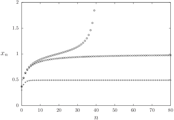
We turn now to the first steps towards the main goal of this article, namely the determination of the asymptotic expansion of $\alpha_{\rm d}(k)$ when $k\to\infty$. Before confronting this functional bifurcation threshold it is much easier to consider the rigidity transition $\alpha_{\rm r}(k)$, that corresponds to the bifurcation of the scalar recursion equation (24). We have given in (25) the expressions that determine analytically $\alpha_{\rm r}(k)$ for all $k$. The value of $\Gamma_{\rm r}(k)$ cannot be given explicitly when $k$ is finite, but it is easy to perform its asymptotic expansion at large $k$, which yields

$$\alpha_{\rm r}(k)=\frac{2^{k-1}}{k}(\ln k+\ln\ln k+\gamma_{\rm r}+o(1))\ ,\qquad\text{with}\ \ \gamma_{\rm r}=1\ .$$

(31)

As explained above this is an upperbound on the sought for dynamic transition $\alpha_{\rm d}(k)$, and the rigorous results of MoReTe11_recclus suggest (or prove for the coloring problem Sly08; SlyZhang16) that the asymptotic expansion of $\alpha_{\rm d}(k)$ has the same form as the one of $\alpha_{\rm r}(k)$, with a different constant term $\gamma_{\rm d}$.

We shall thus study the large $k$ limit taking $\alpha$ to diverge simultaneously with $k$ according to the function $\alpha(k,\gamma)$ defined in Eq. (1), with $\gamma$ a finite constant that becomes our control parameter for the density of constraints in this limit. It is instructive to investigate the behavior of the hard field weights $w_{n}$, solution of the recursion equation (24), for a finite distance $n$. With this choice for the scaling of $\alpha$ with $k$ one easily obtains by induction on $n$ that the leading behavior of $w_{n}$ reads

$$w_{n}=1-\frac{x_{n}}{k\ln k}+o\left(\frac{1}{k\ln k}\right)\ ,$$

(32)

where $x_{n}$ is a $\gamma$-dependent sequence, defined recursively by

$$x_{0}=0\ ,\qquad x_{n+1}=e^{-\gamma+x_{n}}\ .$$

(33)

This recursion function is illustrated on Fig. 4. Its study is very simple, and unveils the following behavior for $x_{n}$: if $\gamma\geq 1$ then $x_{n}$ converges at large $n$ to a finite fixed point (depicted on the right panel of Fig. 5), while for $\gamma<1$ the sequence $x_{n}$ diverges as $n\to\infty$, very quickly (as iterated exponentials). The transition between these two behaviors thus occurs at the critical value of the parameter $\gamma=\gamma_{\rm r}=1$, which corresponds to the expansion of $\alpha_{\rm r}(k)$ stated above. Note that this coincidence is not as trivial as it may look at first sight: the expansion of Eq. (31) was obtained by first taking the limit $n\to\infty$, then $k\to\infty$, while in (33) we have taken the limit $k\to\infty$, and only later studied the behavior of $x_{n}$ for large $n$. The commutativity of these two limits can in this case be traced back to the simple shape of the recursion equation (24): either it has no non-trivial fixed point, or if it has one in the large $k$ limit it must be of order $1-O(1)/(k\ln k)$, and hence captured by the scaling (32).

Our determination of the asymptotic behavior of $\alpha_{\rm d}(k)$ will be based on three hypotheses that we now spell out explicitly. First of all, we assume that this transition occurs on the scale (1), hence that the sought for constant $\gamma_{\rm d}$ can be defined as

$$\gamma_{\rm d}=\lim_{k\to\infty}\left[\frac{k\alpha_{\rm d}(k)}{2^{k-1}}-\ln k-\ln\ln k\right]\ ;$$

(34)

as mentioned above the rigorous results of Sly08; MoReTe11_recclus; SlyZhang16 support this hypothesis. We shall furthermore assume that on this scale of $\alpha$ the order parameter $C(\alpha,k)$ is either equal to 0 (for $\alpha<\alpha_{\rm d}(k)$) or scales with $k$ in the same way as its lowerbound provided by the hard field weight $w(\alpha,k)$ (see Eq. (32)), hence define a reduced order parameter as

$$\widetilde{C}(\gamma)=\lim_{k\to\infty}(1-C(\alpha(k,\gamma),k))k\ln k\ ,$$

(35)

that should be finite for $\gamma>\gamma_{\rm d}$, and diverge to $+\infty$ for $\gamma<\gamma_{\rm d}$. Note that in order to have $\widetilde{C}(\gamma)\geq 0$ we introduced a minus sign in this definition, hence increasing values of $\widetilde{C}$ corresponds to smaller correlations in the original order parameter $C$. Finally we assume that $\widetilde{C}(\gamma)$ can be computed by reversing the order of the large $n$ and large $k$ limits, in other words we define for $n$ finite $\widetilde{C}_{n}(\gamma)$ as

$$\widetilde{C}_{n}(\gamma)=\lim_{k\to\infty}(1-C_{n}(\alpha(k,\gamma),k))k\ln k\ ,$$

(36)

and our third hypothesis will consist in computing $\widetilde{C}(\gamma)$ as the large $n$ limit of $\widetilde{C}_{n}(\gamma)$.

To rephrase these last two hypotheses, we exclude the possibility that on the scale (1) the fixed point order parameter $C(\alpha,k)$ has distinct scalings with $k$ depending on the value of $\gamma$, and similarly that the finite distance correlation function $C_{n}(\alpha,k)$ decays with several plateaus at heights each scaling differently with $k$. These hypotheses are reasonable when confronted with the finite $k$ numerical results (for instance those of Fig. 2), and are somehow corroborated by the scheme of proofs of Sly08; MoReTe11_recclus, that rely on the fact that once $C_{n}$ is “small enough”, then it must decay to 0; we shall see in the rest of the paper that they are at least self-consistent. Note also that they hint at the intrisic difficulty of the computation: in the intermediate regime $[\alpha_{\rm d}(k),\alpha_{\rm r}(k)]$ there are no hard fields in the fixed point distribution $P(h)$, nevertheless the soft fields become asymptotically hard in the $k\to\infty$ limit as the correlation function $C$ tends to 1 according to (35).

References

- (1) M. Garey and D. Johnson. Computers and intractability: A guide to the theory of NP-completeness. Freeman, San Francisco, 1979.
- (2) C. H. Papadimitriou. Computational complexity. Addison-Wesley, 1994.
- (3) R. Monasson, R. Zecchina, S. Kirkpatrick, B. Selman, and L. Troyansky. 2+p-SAT: Relation of typical-case complexity to the nature of the phase transition. Random Structures and Algorithms, 15, 414 (1999).
- (4) G. Biroli, R. Monasson, and M. Weigt. A variational description of the ground state structure in random satisfiability problems. Eur. Phys. J. B, 14, 551 (2000).
- (5) M. Mézard, G. Parisi, and R. Zecchina. Analytic and Algorithmic Solution of Random Satisfiability Problems. Science, 297, 812–815 (2002).
- (6) S. Mertens, M. Mézard, and R. Zecchina. Threshold values of random K-SAT from the cavity method. Random Struct. Algorithms, 28(3), 340–373 (2006).
- (7) F. Krzakala, A. Montanari, F. Ricci-Tersenghi, G. Semerjian, and L. Zdeborova. Gibbs states and the set of solutions of random constraint satisfaction problems. Proceedings of the National Academy of Sciences, 104(25), 10318–10323 (2007).
- (8) D. Achlioptas and F. Ricci-Tersenghi. On the solution-space geometry of random constraint satisfaction problems. In Proc. of 38th STOC, pages 130–139, New York, NY, USA, 2006. ACM.
- (9) D. Achlioptas and A. Coja-Oghlan. Algorithmic barriers from phase transitions. In Proceedings of FOCS 2008, page 793, 2008.
- (10) M. Molloy. The freezing threshold for k-colourings of a random graph. In Proceedings of the 44th symposium on Theory of Computing, page 921. ACM, 2012.
- (11) J. Ding, A. Sly, and N. Sun. Proof of the Satisfiability Conjecture for Large K. In Proceedings of the Forty-seventh Annual ACM Symposium on Theory of Computing, STOC ’15, pages 59–68, 2015.
- (12) M. Mézard and G. Parisi. The Bethe lattice spin glass revisited. Eur. Phys. J. B, 20, 217 (2001).
- (13) A. Montanari and G. Semerjian. Rigorous Inequalities between Length and Time Scales in Glassy Systems. J. Stat. Phys., 125, 23 (2006).
- (14) E. Mossel and Y. Peres. Information flow on trees. Ann. Appl. Probab., 13(3), 817–844 (2003).
- (15) M. Mézard and A. Montanari. Reconstruction on Trees and Spin Glass Transition. J. Stat. Phys., 124, 1317–1350 (2006).
- (16) L. Zdeborová and F. Krzakala. Phase Transitions in the Coloring of Random Graphs. Phys. Rev. E, 76, 031131 (2007).
- (17) L. Dall’Asta, A. Ramezanpour, and R. Zecchina. Entropy landscape and non-Gibbs solutions in constraint satisfaction problems. Phys. Rev. E, 77, 031118 (2008).
- (18) M. Gabrié, V. Dani, G. Semerjian, and L. Zdeborová. Phase transitions in the q-coloring of random hypergraphs. Journal of Physics A: Mathematical and Theoretical, 50(50), 505002 (2017).
- (19) A. Sly. Reconstruction of Random Colourings. Communications in Mathematical Physics, 288(3), 943–961 (2009).
- (20) A. Montanari, R. Restrepo, and P. Tetali. Reconstruction and Clustering in Random Constraint Satisfaction Problems. SIAM Journal on Discrete Mathematics, 25(2), 771–808 (2011).
- (21) A. Sly and Y. Zhang. Reconstruction of colourings without freezing. arXiv preprint arXiv:1610.02770, (2016).
- (22) G. Semerjian. On the freezing of variables in random constraint satisfaction problems. J. Stat. Phys., 130, 251 (2008).
- (23) A. Montanari, F. Ricci-Tersenghi, and G. Semerjian. Clusters of solutions and replica symmetry breaking in random k-satisfiability. J. Stat. Mech., P04004 (2008).
- (24) F. R. Kschischang, B. Frey, and H.-A. Loeliger. Factor graphs and the sum-product algorithm. IEEE Trans. Inform. Theory, 47(2), 498–519 (2001).
- (25) T. Richardson and R. Urbanke. Modern Coding Theory. Cambridge University Press, 2007.
- (26) H. Nishimori. Statistical Physics of Spin Glasses and Information Processing: An Introduction. Oxford University Press, Oxford, UK, 2001.
- (27) R. Abou-Chacra, D. J. Thouless, and P. W. Anderson. A selfconsistent theory of localization. Journal of Physics C: Solid State Physics, 6(10), 1734 (1973).
- (28) A. Braunstein, M. Mézard, and R. Zecchina. Survey propagation: An algorithm for satisfiability. Random Struct. Algorithms, 27(2), 201–226 (2005).
- (29) K.-I. Sato. Lévy Processes and Infinitely Divisible Distributions. Cambridge University Press, 2013.
- (30) S. Asmussen and J. Rosinski. Approximations of small jumps of Lévy processes with a view towards simulation. Journal of Applied Probability, 38(2), 482–493 (2001).
- (31) Z. Chi. Nonnormal Small Jump Approximation of Infinitely Divisible Distributions. Advances in Applied Probability, 46(4), 963–984 (2014).
- (32) W. Feller. An introduction to probability theory and its applications, Vol II, 2nd ed. Wiley New York, 1971.
- (33) T. Watanabe and K. Yamamuro. Ratio of the Tail of an Infinitely Divisible Distribution on the Line to that of its Lévy Measure. Electron. J. Probab., 15, 44–74 (2010).
- (34) G. R. Brightwell and P. Winkler. A second threshold for the hard-core model on a Bethe lattice. Random Structures & Algorithms, 24(3), 303–314 (2004).
- (35) J. Barbier, F. Krzakala, L. Zdeborová, and P. Zhang. The hard-core model on random graphs revisited. Journal of Physics: Conference Series, 473, 012021 (2013).
- (36) N. Bhatnagar, A. Sly, and P. Tetali. Reconstruction Threshold for the Hardcore Model. In M. Serna, R. Shaltiel, K. Jansen, and J. Rolim, editors, Approximation, Randomization, and Combinatorial Optimization. Algorithms and Techniques, pages 434–447, 2010.
- (37) L. Budzynski, F. Ricci-Tersenghi, and G. Semerjian. Biased landscapes for random constraint satisfaction problems. Journal of Statistical Mechanics: Theory and Experiment, 2019(2), 023302 (2019).