On the separation of shape and temporal patterns in time series
-Application to signature authentication-

We consider the following $\mathcal{G}$ class of stochastic generative processes that can be formalized in a parametric form:

with $t\in\{0,1,2,\cdots\}$ the discrete time variable, $\xi\in\Xi$ a function, possibly stochastic, monotonously increasing with $t$, $G\in\Gamma$ a nonlinear function randomly drawn from $\Gamma$, $o(t)$ the observable output of the process at timestamps $t$ and $\epsilon$ a Gaussian noise with zero mean and standard deviation $\sigma$. We will denote such process $(\Gamma,\Xi,\epsilon_{\sigma})$.

The set $\Gamma$ will characterize what we call the shape variability and the set $\Xi$ the temporal variability.

Thus, if we observe $N$ distinct realizations of the previous generative process, we get a set of $N$ traces $\{o_{i}(t)\}_{i=1,\cdots,N}$ such that:

with $G_{i}\in\Gamma$, $\xi_{i}\in\Xi$ and $\epsilon_{i}$ a Gaussian noise.

In the absence of a strictly atemporal shape, we will call (temporally) neutral shape associated to the process defined by Eq.4 the time series $O_{s}(t)=E(G(E(\xi(t))))$, where $E$ represents the mathematical expectation, and $t\in\{0,1,2,\cdots\}$. For the neutral shape, the associated temporal function $\xi_{s}(t)$ corresponds to the mathematical expectation of observed $\xi$ functions.

As an example, the stochastic process defined by

1. 1.

   matrix $G_{a,b}$ defined in Eq. 5,

2. 2.

   $\xi_{\omega}(t)=\omega\cdot t$,

3. 3.

   constraints on the parameters, $a=a_{0}\cdot(1+U_{[-.5,.5]})$, $b=b_{0}\cdot(1+U_{[-.5,.5]})$,
   $\omega=\omega_{0}\cdot(1+U_{[-.1,.1]})$, $\varphi=\varphi_{0}+U_{[-.1,.1]}$ where $U_{[u,v]}$ is the uniform law defined on interval $[u,v]$, and

4. 4.

   the additive Gaussian noise $\epsilon_{\sigma}(t)$,

belongs to the $\mathcal{G}$ class of process, sets $\Gamma$ and $\Xi$ being respectively defined by the constraints on $(a,b)$ and $(\omega,\varphi)$ parameters.

Here, $\Gamma=\{G_{a,b}|a=a_{0}\cdot(1+U_{[-.25,.25]}),b=b_{0}\cdot(1+U_{[-.25,.25]})\}$ and $\Xi=\{\omega t+\varphi|\omega=\omega_{0}\cdot(1+U_{[-.1,.1]}),\varphi=\varphi_{0}+U_{[-.25,.25]}\}$.

The neutral shape for this process is $O_{s}(t)=G_{a_{0},b_{0}}(\omega_{0}t+\varphi_{0})$.

Given $\{o_{i}(t)\}_{i=1,2,\cdots,N}$, $N$ observations assumed to be produced by a stochastic process class $\mathcal{G}$,

Can we estimate $\Gamma$, $\Xi$, $O_{s}$ and $\{\xi_{i}(t)\}_{i=1,2,\cdots,N}$ under the conditions that $\forall i$, $o_{i}(t)=G_{i}(\xi_{i}(t))+\epsilon_{i}(t)$, $G_{i}\in\Gamma$, $\xi_{i}\in\Xi$ and $\epsilon_{i}$ a Gaussian noise with zero mean?

Answering this question is to separate the neutral shape from the temporal functions. This separation makes it possible to consider the study of shape variability independently of temporal variability.

The general problem of separability as previously stated is under-constrained (or ill-posed) and, as such, probably does not admit a solution in the general case. On the other hand, we empirically show that the algorithm proposed in [5] that estimates an average time series of a set of time series using temporally elastic kernel provides a way to approximate the concept of neutral shape. Moreover, the probabilistic formalization of the temporal alignment mechanism that is suggested is particularly suited to address our separation problem.

We present below the general concepts of this algorithm (for details, see [5]) and show how it offers elements of answer to the previously stated problem of separability.

Unlike the dynamic time warping algorithm (DTW) [6] which considers only the best alignment path to match pairs of time series, the time elastic kernels [7, 8] consider the sum of the alignment scores of all possible matching paths. The score assigned to a path is the result of the product of the local matching kernels evaluated along the path.

Let $o_{1}^{n}=o_{1}o_{2}\cdots o_{n}$ and ${o^{\prime}}_{1}^{n^{\prime}}=o^{\prime}_{1}o^{\prime}_{2}\cdots o^{\prime}_{n^{\prime}}$ be two time series (observations) with respective lengths $n$ and $n^{\prime}$. The local kernel that quantifies the proximity of two samples $o_{i}$ and $o^{\prime}_{j}$ is in general an exponential kernel : $k(o_{i},o^{\prime}_{j})=e^{-\nu\cdot||o_{i},o^{\prime}_{j}||^{2}}$. By interpreting this local kernel as a local probability function [5], it is possible to consider the alignment of two time series as the mathematical expectation of the outputs generated by a stochastic finite state machinery.

The considered stochastic automata is a Hidden Markov process defined on a finite set of hidden states $\mathcal{S}=\{S_{1,1},S_{1,2},\cdots,S_{n,n^{\prime}},S_{n+1,n^{\prime}+1}\}$. Each state $S_{i,j}$ characterizes the alignment between two samples $o_{i}$ and $o^{\prime}_{j}$, $S_{1,1}$ is assimilated to the initial state and $S_{n,n^{\prime}}$ as the final state.

The hidden variable (at step $\tau$) $z_{\tau}$ takes value in $\mathcal{S}$. The index $\tau$ follows one of the admissible alignment paths and takes value in $\{(1,1),...,(n,n^{\prime})\}$. To take into account monotonic alignment constraints (as in DTW), we impose $\tau=(i,j)$, $\tau+1\in\{(i,j+1),(i+1,j),(i+1,j+1)\}$ and $\tau-1\in\{(i,j-1),(i-1,j),(i-1,j-1)\}$.

The a posteriori probability for the process to be in state $S_{i,j}$ at step $\tau$, given the observed sequences $o_{1}^{n}$ et ${o^{\prime}}_{1}^{n^{\prime}}$ est $P(z_{\tau}=S_{i,j}|o_{1}^{n},{o^{\prime}}_{1}^{n^{\prime}},\theta)$, where $\theta$ is the vector of parameters of the Hidden Markov Model. This a posteriori probability is estimated through forward and backward recursions, $\alpha$ and $\beta$ defined as follows

$\alpha_{\tau}(t,t^{\prime})=P(o_{1}^{t},{o^{\prime}}_{1}^{t^{\prime}},z_{\tau}=S_{t,t^{\prime}}|\theta)$ is the probability for the process to be at state $S_{t,t^{\prime}}$ at step $\tau$ once the partial observation sequences $(o_{1}^{t},{o^{\prime}}_{1}^{t^{\prime}})$ are aligned.
$\beta_{\tau}(t,t^{\prime})=P(o_{t}^{n},{o^{\prime}}_{t^{\prime}}^{n^{\prime}}|z_{\tau}=S_{t,t^{\prime}},\theta)$ is the probability of the alignment of the pair of partial sequences $(o_{t}^{n},{o^{\prime}}_{t^{\prime}}^{n^{\prime}})$ given the alignment process is at state $S_{t,t^{\prime}}$ at step $\tau$.

The matching of any pair of samples $o_{i}$ and $o^{\prime}_{j}$ can then be interpreted as the probability of presence of the stochastic alignment automata on cell $S_{i,j}$.

The marginal probability for the process to be at step $\tau$ in one of the states of the subset $S_{t,\bullet}=\{S_{t,1},S_{t,2},\cdots,S_{t,n^{\prime}}\}$, being given the observations $o_{1}^{n}$ and ${o^{\prime}}_{1}^{n^{\prime}}$, (that is, the probability for the process to visit at step $\tau$ one of the state of $S_{t,\bullet}$, or $o_{t}$ to be aligned with one of the samples in the series ${o^{\prime}}_{1}^{n^{\prime}}$) is given by:

The mathematical expectation of alignments of samples in the ${o^{\prime}}_{1}^{n^{\prime}}$ series with the sample $o_{t}$ (given that $o_{t}$ is aligned by the automaton) and similarly the expectation of the time occurrences associated with the samples of the series ${o^{\prime}}_{1}^{n^{\prime}}$ aligned with $o_{t}$ are defined by:

The previous mathematical expectations (Eq. 8) are the basis of the proposed procedure for estimating a time elastic centroid for a set of time series.

Let $\mathcal{O}=\{{}^{k}\!o_{1}^{n_{k}}\}_{k=1\cdots N}$ be a subset of time series, $r_{1}^{n}$ a reference time series ($r_{1}^{n}$ can be initialized with the medoid of $\mathcal{O}$). The centroid estimate of $\mathcal{O}$ is defined by the tuple $(O_{s},\xi_{s})$ where $O_{s}$ is a time series of length $n$ and $\xi_{s}$ is the sequence of time occurrences associated to the sample of $O_{s}$

$(O_{s},\xi_{s})$ is in general a non-uniformly sampled time series: $\xi_{s}(t)$ is the mathematical expectation of the time of occurrence for sample $O_{s}(t)$. If necessary, a uniform re-sampling can straightforwardly be used to get back to a uniformly sampled time series.

By successive iterations, i.e. by replacing the reference time series $r_{1}^{n}$ by the new centroid estimates $O_{s}$ evaluated at the end of each iteration, until no more improvement can be obtained (decrease in inertia), we get a final estimate of the centroid for $\mathcal{O}$.

It should be noted here that the underlying multiple alignment problem being NP-complete [9] and characterized with an exponential complexity [10] with the size of $\mathcal{O}$, only sub-optimal heuristics allow to approach this notion of temporally elastic centroid for sets $\mathcal{O}$ of more than tens of time series.

We conjecture that, at the end of the iterative process, $(O_{s},\xi_{s})$ as defined by the equations Eq.9 is an empirical estimator for the neutral shape associated to the set $\mathcal{O}$. Furthermore, equations 8 also provide access to temporal function estimators $\xi_{i}$ associated with the elements of $\mathcal{O}$. Thus, for $o_{i}={o_{i}}_{1}^{n_{i}}\in\mathcal{O}$, and the neutral shape $O_{s}$ estimated on $O$, the estimate of the temporal function $\xi_{i}$ associated with $o_{i}$ is:

In other words, each $\xi_{i}(t)$ corresponds to the mathematical expectation of the alignment times of the samples of the series $o_{i}$ with the sample $O_{s}(t)$ of the neutral form.

In terms of algorithmic complexity, this algorithm is in $O(|\mathcal{O}|.||O_{s}||^{2})$, that is to say quadratic with respect to the average size of the time series and therefore of the size $|O_{s}|$ of the neutral form, and linear with respect to the cardinal of $\mathcal{O}$.

We take again the ellipse example, previously introduced in subsection II-A, and characterized by the process $g\in\mathcal{G}$ defined through equation 5 with the following parameter values: $\omega_{0}=2\pi f_{0}$ with $f_{0}=1hz$ and $fe=400hz$ the sampling frequency, $\varphi_{0}=0$, $a_{0}=2$, $b_{0}=1$, all the ellipses being centered in $(1,.5)$, $\epsilon$ a Gaussian noise with standard deviation $\sigma=1.5$.

A subset of $20$ time series is produced by $g$ from which the separation of shape and time functions is evaluated. The results of the separation process are shown in Fig. 1.

To illustrate the variability of (non-noisy) shapes produced by $g$, the sub-figure at the top left shows the projections of the 20 ellipses randomly generated by $g$. At the bottom right sub-figure, are presented i) the noisy trajectories of the time series produced by $g$ (cyan curves), the theoretical neutral (mean) shape (dashed red curve) and the neutral shape estimate (black curve) provided by our algorithm.

At the top center, the sub-figure presents the temporal variability by displaying the 20 true $\xi_{i}$ temporal functions associated with the previous shapes. The sub-figure at the bottom center shows the estimated temporal functions $\xi_{i}$, the red curve corresponding to the mean time curve associated with the neutral shape.

Finally, the right sub-figures present new temporal functions produced by $g$ that violate the temporal constraints previously fixed. The true temporal functions are shown in the top sub-figure, while the estimated temporal function are shown in the bottom sub-figure. The red curve corresponds to the neutral temporal curve $\xi_{s}$ associated to the neutral shape $O_{s}$ ($f0=1hz$). The cyan color curve corresponds to the estimate of a function $\xi$ generated with a frequency $f$ that is twice higher than $f_{0}$ ($f=2hz$). The shape is thus traveled twice as fast and the slope expected for the cyan curve is twice times lower than that of the red curve, which is approximately the case for the estimation displayed in the figure. The black curve corresponds to the estimate of a function $\xi$ generated with a frequency $f$ twice as small as $f0$ ($f=0,5hz$). The shape is therefore traveled half as fast as the neutral shape, and the expected slope for the black curve is twice times greater than that of the red curve, which is approximately the case for the estimation presented in the figure. The blue dashed curves correspond to temporal curves presenting constant acceleration (below the red curve) and deceleration (above the red curve). The shapes of these two curves are no longer linear, which is also expected. Finally, the dashed green curve corresponds to a frequency modulated $xi$ curve, which thus presents successive accelerations and decelerations. The fluctuations are not very well reproduced in the estimation of this curve, but they are nevertheless quite visible in the temporal curve that is extracted by our algorithm.

This simple synthetic example, which nevertheless presents a relatively important temporal and shape variability coupled with an additive noise largely covering the neutral shape, shows that the initial objective behind this notion of separation of shape and time components within time series has some empirical grounds. The concept of time elastic centroid makes it possible, on this example, to approach this concept of neutral shape and furthermore allows for the extraction of the temporal functions associated to the shape utterances that are randomly produced by a stochastic generative process $g$.

We are interested here in some experiments related to the identification of forgeries of some online genuine signatures. These signatures are collected using capture devices such as digitizing tables, digital pens or touch screens. The data is in the form of trajectories in $\mathbb{R}^{d}$, with $d\geq 2$ (including at least positions $x$ and $y$, and possibly pressure sensor output, stylus or pen orientations, etc.)

The tasks we consider are semi-supervised classification tasks that can be considered as being similar to anomaly detection tasks: only a few legitimate signatures are available for learning, forgery signatures can be considered as anomalies with respect to legitimate signatures.

The approach developed here consists in applying the separation algorithm on the training set, that is to say, to extract from legitimate signatures the neutral shape component and the temporal functions. From these shape and time components, we then construct an overall dissimilarity score between a test signature and our model that integrates a measure of shape dissimilarity and a measure of temporal dissimilarity.

The shape dissimilarity between a test time series $o$ and the neutral shape $O_{s}$ is estimated by evaluating the mean squared error of the differences between the samples of the neutral shape $O_{s}(t)$ and the mathematical expectations of the samples of time series $o$ that are aligned with $O_{s}(t)$, as formalized by equation Eq. 11.

The temporal dissimilarity is composed of the product of two terms, as specified by equation Eq. 12. The first term evaluates the absolute difference between the normalized averaged slope of temporal function $\xi_{o}$ and unity. The averaged slope is obtained by a linear regression estimated on the temporal function. It is normalized using the mean slope $\overline{Slope}$ estimated on the linear regressions of the temporal function extracted from the training time series (which corresponds to legitimate signatures).

The second term evaluates the absolute difference to unity of the area under the curve (AUC) for temporal function $\xi_{o}$ normalized by the mean AUC, noted $\overline{AUC}$, of the $\xi$ functions extracted on the training data.

The global dissimilarity score correspond to the fusion of the two previous terms as specified in equation Eq.13. The meta parameter $\alpha$ is used to adjust weight of importance between temporal and shape dissimilarities. This method for separating shape and temporal functions in time series along with the subsequent score aggregation model is call STS (shape and time separation) in the remaining part of the article.

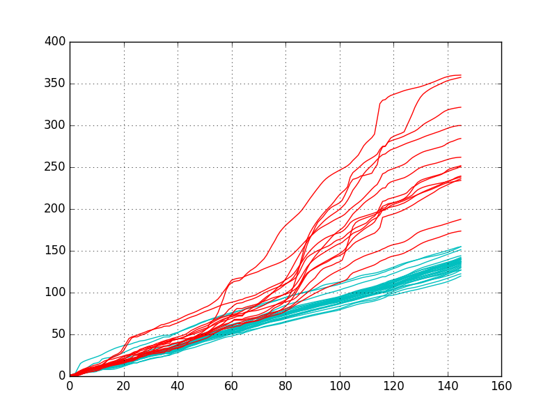
As an illustration, we present in Fig. 2, the result of our separating algorithm applied on a case extracted from the MOBISIG dataset presented below. On the top left sub-figure, the dark blue trajectory corresponds to the neutral shape, superimposed to the curves that correspond to the legitimate signatures used for training. On the top right sub-figure, temporal functions extracted from legitimate signatures are shown in cyan color, while temporal functions extracted from forgery signatures are shown in red color. On this example, most of the forgeries are characterized with a highly nonlinear temporal function, whose slope greatly increases near the middle of the signature realization. Moreover, comparatively to genuine signatures, forgeries are produced with slower temporal patterns. Clearly, on this example, the average slopes and AUCs are significantly higher for forgeries than for genuine signatures.

In Fig. 2, bottom sub-figure, we show the 2D distributions corresponding to the dissimilarity scores, with the temporal dissimilarity in the x-axis and the shape dissimilarity in the y-axis. One can notice that, for the legitimate signatures (blue, cyan cluster), this 2D distribution is much more compact than it is for the 2D distribution associated to forgeries (red cluster). Furthermore, on this example, using the two dissimilarity scores jointly enable us to find a better separating hyperplane between the two clusters comparatively to the case where only one of the two scores is considered.

For the considered benchmarks, the assessment measures that are used are the following ones:

1. 1.

   EER : (equal error rate) gives the error rate obtained when the false-positive rate is equal to the false-negative rate. In this configuration, rates are evaluated globally, i.e. when all subjects are treated together, without distinction.

2. 2.

   aEER : (equal error rate) gives the average error rate obtained when the false-positive rate is equal to the false-negative rate. In this configuration, rates are evaluated subject by subject and then averaged.

3. 3.

   FAR et FRR : true False Acceptance Rate and False Rejection Rate obtained when operating at the closest to the EER point.
   

The SVC2004 [11] dataset is the first benchmark specifically designed for evaluating on-line handwritten signature verification systems. SVC2004 contains two distinct tasks: the first task only exploits the 2D (x,y) trajectories that are captured using a digitizing tablet (WACOM Intuos tablet) with a $100hz$ sampling frequency as well as the pen-down/pen-up binary information, that tells whether the contact between the pen and the tablet is established or not. The second task exploits supplementary information including the orientation of the pen. We have used the first task to determine a satisfactory value for meta parameter $\alpha$ (cf. Eq. 13). Using a cross-validation we have obtained best EER values in average for $\alpha=.85$. This $\alpha$ value has been used (and maintain constant) to evaluate the STS approach on the second MOBISIG task as well as for the processing of all the other benchmarks described below.

The ICDAR2011 dataset [12] is made of 3D trajectories $(x,y,z)$, produced by 10 subjects and captured using digitizing tablet Intuos3 (with a sampling frequency of $200hz$) and a pen. Here $z$ contains the pressure exerted on the pen.

The MOBISIG dataset [13] is made of pseudo-signatures produced by 83 subjects using one of their fingers and captured using a mobile tablet equipped with a touch screen. The signatures are captured with a sampling frequency of $60hz$. The collected trajectories contain 2D positions $x$ and $y$, the speeds $vx$ and $vy$, accelerations $ax$ and $ay$ the pressure exerted on the touch screen $z$, and the size of the contact area between the finger and the screen $ta$. We have applied the STS approach on the trajectories containing the previous features, without using the accelerations or the speeds dimensions that are more or less already encoded into the temporal functions we are extracting.

The pre-processing that has been implemented is common to all the datasets. Basically we remove the mean and normalized the data using standard deviations for $x$, $y$ and $z$ (the pen pressure). The other dimensions, if any, are normalized into the unit interval using $u=(u-min_{u})/(max_{u}-min_{u})$.

Table Tab. I presents in a synthetic way results that have been obtained on the three benchmarks that cover four distinct tasks. Our algorithm (STS) achieves slightly better results than the best methods that have been evaluated so far on these tasks. These results are quite encouraging since the nature of the capture devices as well as the cultural differences of the subjects (European and Asian) are relatively diversified. The state of the art is mostly composed with methods that are derived from DTW for SVC2004 and MOBISIG benchmarks, and with statistical methods or heuristics-based approaches that are not detailed for the ICDAR2011 benchmark. Neural-based approaches, particularly those involving deep learning or recurrent architectures, seem poorly suited to these tasks because of the limited size of the training sets.

The C++ code with a Python wraper is available at
https://github.com/pfmarteau/ShapeTimeSeparation/.

References

- [1] A. Andreopoulos and J. K. Tsotsos, “50 years of object recognition: Directions forward,” Computer Vision and Image Understanding, vol. 117, no. 8, pp. 827 – 891, 2013.
- [2] V. Niennattrakul, D. Srisai, and C. A. Ratanamahatana, “Shape-based template matching for time series data,” Knowledge-Based Systems, vol. 26, pp. 1 – 8, 2012.
- [3] V. M. Panaretos and Y. Zemel, “Amplitude and phase variation of point processes,” The Annals of Statistics, vol. 44, no. 2, p. 771?812, Apr 2016. [Online]. Available: http://dx.doi.org/10.1214/15-AOS1387
- [4] L. M. Sangalli, P. Secchi, S. Vantini, and V. Vitelli, “k-mean alignment for curve clustering,” Computational Statistics and Data Analysis, vol. 54, no. 5, pp. 1219 – 1233, 2010. [Online]. Available: http://www.sciencedirect.com/science/article/pii/S0167947309004605
- [5] P.-F. Marteau, “Times series averaging and denoising from a probabilistic perspective on time-elastic kernels,” International Journal of Applied Mathematics and Computer Science, vol. 29, no. 2, pp. 375–392, Jun. 2019. [Online]. Available: https://hal.archives-ouvertes.fr/hal-01401072
- [6] H. Sakoe and S. Chiba, “A dynamic programming approach to continuous speech recognition,” in Proceedings of the Seventh International Congress on Acoustics, Budapest, vol. 3. Budapest: Akadémiai Kiadó, 1971, pp. 65–69.
- [7] M. Cuturi, J.-P. Vert, O. Birkenes, and T. Matsui, “A kernel for time series based on global alignments,” in IEEE ICASSP 2007, vol. 2, April 2007, pp. II–413–II–416.
- [8] P.-F. Marteau and S. Gibet, “On Recursive Edit Distance Kernels with Application to Time Series Classification,” IEEE Trans. on Neural Networks and Learning Systems, pp. 1–14, Jun. 2014.
- [9] L. Wang and T. Jiang, “On the complexity of multiple sequence alignment.” Jour. of Comp. Biology, vol. 1, no. 4, pp. 337–348, 1994.
- [10] W. Just and W. Just, “Computational complexity of multiple sequence alignment with sp-score,” Journal of Computational Biology, vol. 8, pp. 615–623, 1999.
- [11] D. yan Yeung, H. Chang, Y. Xiong, S. George, R. Kashi, T. Matsumoto, and G. Rigoll, “Svc2004: First international signature verification competition,” in In Proceedings of the International Conference on Biometric Authentication (ICBA), Hong Kong. Springer, 2004, pp. 16–22.
- [12] M. Liwicki, M. I. Malik, C. E. v. d. Heuvel, X. Chen, C. Berger, R. Stoel, M. Blumenstein, and B. Found, “Signature verification competition for online and offline skilled forgeries (sigcomp2011),” in 2011 International Conference on Document Analysis and Recognition, Sep. 2011, pp. 1480–1484.
- [13] M. Antal, L. Z. Szabó, and T. Tordai, “Online signature verification on mobisig finger-drawn signature corpus,” Mobile Information Systems, vol. v, pp. 1–15, 2018.
- [14] A. Sharma and S. Sundaram, “An enhanced contextual dtw based system for online signature verification using vector quantization,” Pattern Recogn. Lett., vol. 84, no. C, pp. 22–28, Dec. 2016. [Online]. Available: https://doi.org/10.1016/j.patrec.2016.07.015