Robustness Certificates for Sparse Adversarial Attacks by Randomized Ablation

Adversarial attacks, and defenses against these attacks, have been active topics of research in machine learning in recent years [\citeauthoryearSzegedy et al.2013, \citeauthoryearCarlini and Wagner2017, \citeauthoryearMadry et al.2017]. In the case of image classification, given a classifier $f$, the goal of an adversarial attack on an image ${\mathbf{x}}$ is to produce an image ${\mathbf{x}}^{\prime}$, such that ${\mathbf{x}}^{\prime}$ is visually similar to ${\mathbf{x}}$, but $f$ classifies ${\mathbf{x}}^{\prime}$ differently than it classifies ${\mathbf{x}}$. Assuming that ${\mathbf{x}}$ is a natural image that was classified correctly, this means that the attacker can produce an image ${\mathbf{x}}^{\prime}$ which looks imperceptibly similar to this natural image, but is misclassified by $f$.
When designing or evaluating an adversarial attack, one must choose an objective measure of ‘similarity’ between two images: more precisely, the goal of the attacker is to minimize $d({\mathbf{x}},{\mathbf{x}}^{\prime})$, subject to $f({\mathbf{x}})\neq f({\mathbf{x}}^{\prime})$, where $d$ is a chosen distance metric. Most existing work in adversarial examples has used $L_{p}$ norms as distance metrics, focusing in particular on $L_{\infty}$ and $L_{2}$ norms [\citeauthoryearGoodfellow, Shlens, and Szegedy2015, \citeauthoryearSzegedy et al.2013, \citeauthoryearMadry et al.2017, \citeauthoryearDong et al.2018, \citeauthoryearKurakin, Goodfellow, and Bengio2018]. The $L_{0}$ metric, which is simply the number of pixels at which ${\mathbf{x}}^{\prime}$ differs from ${\mathbf{x}}$, has also been the target of adversarial attacks. This metric presents a distinct challenge, because $d({\mathbf{x}},{\mathbf{x}}^{\prime})$ is non-differentiable. However, both gradient-based (white-box) attacks [\citeauthoryearMadry et al.2017, \citeauthoryearPapernot et al.2016a] and zeroth-order (black-box) attacks [\citeauthoryearSchott et al.2019] have been proposed under the $L_{0}$ attack model. The $L_{0}$ attack model is the focus of this paper.
Several practical defenses against adversarial attacks under the $L_{0}$ attack model have been proposed in the last couple of years. These methods include defensive distillation [\citeauthoryearPapernot et al.2016b], as well as attempts to recover ${\mathbf{x}}$ from ${\mathbf{x}}^{\prime}$ using compressed sensing [\citeauthoryearBafna, Murtagh, and Vyas2018] or generative models [\citeauthoryearSchott et al.2019, \citeauthoryearMeng and Chen2017]. However, as new defenses are proposed, new attacks are also developed for which these defenses are vulnerable (e.g. [\citeauthoryearCarlini and Wagner2016]). Experimental demonstrations of a defense’s efficacy based on currently existing attacks do not provide a general proof of security. In response, certifiably robust classifiers have been developed for adversarial examples for a variety of attack models [\citeauthoryearWong and Kolter2018, \citeauthoryearGowal et al.2018]. For these classifiers, given an image ${\mathbf{x}}$, it is possible to compute a radius $\rho$ such that it is guaranteed that no adversarial example ${\mathbf{x}}^{\prime}$ exists within a distance $\rho$ of ${\mathbf{x}}$. One drawback of many of these certifiable approaches is that they can be computationally expensive since they attempt to minimize $d({\mathbf{x}},{\mathbf{x}}^{\prime})$ (or its lower bound) using formal methods.
Recently, a relatively computationally inexpensive family of certifiably robust classifiers have been proposed which employ randomized smoothing [\citeauthoryearLecuyer et al.2019, \citeauthoryearCohen, Rosenfeld, and Kolter2019, \citeauthoryearLi et al.2018, \citeauthoryearSalman et al.2019]. This development has mostly been focused on the $L_{1}$ and $L_{2}$ metrics. Conceptually, these schemes work by repeatedly adding random noise to the image ${\mathbf{x}}$, in order to create a large set of noised images. A base classifier is then used to classify each of these noised samples, and the final robust classification is made by ‘majority vote.’ The key insight is that, if the magnitude of the noise added to each image is much larger than the distance between ${\mathbf{x}}$ and a potentially adversarial image ${\mathbf{x}}^{\prime}$, then any particular noised image generated from ${\mathbf{x}}$ could have been generated from ${\mathbf{x}}^{\prime}$ with nearly equal likelihood. Then the expected number of ‘votes’ for each class can only differ between ${\mathbf{x}}$ and ${\mathbf{x}}^{\prime}$ by a bounded amount. Therefore, if we use a statistically sufficient number of random noise samples, and if the observed ‘gap’ between the number of votes for the top class and the number of ‘votes’ for any other class at ${\mathbf{x}}$ is sufficiently large, then we can guarantee with high probability that the robust classification at ${\mathbf{x}}^{\prime}$ will be the same as it is at ${\mathbf{x}}$. Note that the success probability can be made arbitrarily high by adding more noise samples to ${\mathbf{x}}$ in the smoothing process.
In this work, we develop a certifiably robust classification scheme for the $L_{0}$ metric (i.e. sparse adversarial perturbations). To guarantee the robustness of the classification against sparse adversarial attacks, we propose a novel smoothing method based on performing random ablations on the input image, rather than adding random noise. In our proposed $L_{0}$ smoothing method, for each sample generated from ${\mathbf{x}}$, a majority of pixels are randomly dropped from the image before the image is given to the base classifier. If a relatively small number $\rho$ of pixels have been adversarially corrupted (which is the case in sparse adversarial attacks), then it is highly likely that none of these pixels are present in a given ablated sample. Then, for the majority of possible random ablations, ${\mathbf{x}}$ and ${\mathbf{x}}^{\prime}$ will give the same ablated image. Therefore, the expected number of votes for each class can only differ between ${\mathbf{x}}$ and ${\mathbf{x}}^{\prime}$ by a bounded amount. Using this, we can prove that with high probability, the smoothed classifier will classify ${\mathbf{x}}$ robustly against any sparse adversarial attack which is allowed to perturbed certain number of input pixels, provided that the ‘gap’ between the number of votes for the top class and the number of ‘votes’ for any other class at ${\mathbf{x}}$ is sufficiently large. (See Figure 1)
Our ablation method produces significantly larger robustness guarantees compared to a more direct extension of randomized smoothing to the $L_{0}$ metric provided in a concurrent work by [\citeauthoryearLee et al.2019]: see the Discussion section for a comparison of the techniques.
We note that our proposed approach bears some similarities to [\citeauthoryearHosseini, Kannan, and Poovendran2019], in that both works aim to defend against $L_{0}$ adversarial attacks by randomly ablating pixels. However, several differences exist: most notably, [\citeauthoryearHosseini, Kannan, and Poovendran2019] presents a practical defense with no robustness certificate given. By contrast, the main contribution of this work is a provable guarantee of robustness to adversarial attack.
In summary, our contributions are as follows:

• •

  We develop a novel defense technique against sparse adversarial attacks (threat models that use the $L_{0}$ metric) based on randomized ablation.

• •

  We characterize robustness guarantees for our proposed defense against arbitrary sparse adversarial attacks.

• •

  We show the effectiveness of the proposed technique on standard datasets: MNIST, CIFAR-10, and ImageNet.

We will use ${\mathcal{S}}$ to represent the set of possible pixel values in an image. For example, in an 24-bit RGB color image, ${\mathcal{S}}=\{0,1,...,255\}^{3}$, while in a binarized black-and-white image, ${\mathcal{S}}=\{0,1\}$. We will use ${\mathcal{X}}={\mathcal{S}}^{d}$ to represent the set of possible images, where $d$ is the number of pixels in each image. Additionally, we will use ${\mathcal{S}_{{\text{NULL}}}}$ to represent the set ${\mathcal{S}}\cup\{{\text{NULL}}\}$, where NULL is a null symbol representing the absence of information about a pixel, and ${\mathcal{X}_{{\text{NULL}}}}={\mathcal{S}_{{\text{NULL}}}}^{d}$ to represent the set of images where some elements in the images may be replaced by the null symbol. Note that NULL is not the same as a zero-valued pixel, or black. For example, if ${\mathcal{S}}=\{0,1\}$ and $d=5$, then $[0,1,1,0,1]^{T}\in{\mathcal{X}}$, while $[{\text{NULL}},1,{\text{NULL}},0,1]^{T}\in{\mathcal{X}_{{\text{NULL}}}}$.
Also, let $[d]$ represent the set of indices $\{1,...,d\}$, let ${\mathcal{H}}(d,k)\subseteq{\mathcal{P}}([d])$ represent all sets of $k$ unique indices in $[d]$, and let ${\mathcal{U}}(d,k)$ represent the uniform distribution over ${\mathcal{H}}(d,k)$. (To sample from ${\mathcal{U}}(d,k)$ is to sample $k$ out of $d$ indices uniformly without replacement. For example, an element sampled from ${\mathcal{U}}(5,3)$ might be $\{2,4,5\}$.)
We define the operation ${{\textsc{Ablate}}}\in{\mathcal{X}}\times{\mathcal{H}}(d,k)\to{\mathcal{X}_{{\text{NULL}}}}$, which takes an image and a set of indices, and outputs the image, with all pixels except those in the set replaced with the null symbol NULL. For example, ${{\textsc{Ablate}}}([0,1,1,0,1]^{T},\{2,4,5\})=[{\text{NULL}},1,{\text{NULL}},0,1]^{T}$
For images ${\mathbf{x}},{\mathbf{x}}^{\prime}\in{\mathcal{X}}$, let $\|{\mathbf{x}}-{\mathbf{x}}^{\prime}\|_{0}$ denote the $L_{0}$ distance between ${\mathbf{x}}$ and ${\mathbf{x}}^{\prime}$, defined as the number of pixels at which ${\mathbf{x}}$ and ${\mathbf{x}}^{\prime}$ differ. Note that we are following the convention used by [\citeauthoryearCarlini and Wagner2017], where, for a color image, the number of channels in which the images differ at a given pixel location does not matter: any difference at a pixel location (corresponding to an index in $[d]$) counts the same. This differs from [\citeauthoryearPapernot et al.2016a], in which channels are counted separately. Also (in a slight abuse of notation) let ${\mathbf{x}}\ominus{\mathbf{x}}^{\prime}$ denote the set of pixel indices at which ${\mathbf{x}}$ and ${\mathbf{x}}^{\prime}$ differ, so that $\|{\mathbf{x}}-{\mathbf{x}}^{\prime}\|_{0}=|{\mathbf{x}}\ominus{\mathbf{x}}^{\prime}|$.
Finally, for multiclass classification problems, let $c$ be the number of classes.

First, we note that in this section, we closely follow the notation of [\citeauthoryearCohen, Rosenfeld, and Kolter2019], using appropriate analogs between the $L_{2}$ smoothing scheme of that work, and the proposed $L_{0}$ ablation scheme of this work. In particular, let $f\in{\mathcal{X}_{{\text{NULL}}}}\rightarrow[c]$ denote a base classifier, which is trained to classify images with some pixels ablated. Let $g\in{\mathcal{X}}\rightarrow[c]$ represent a smoothed classifier, defined as:

where $k$ is the retention constant; i.e., the number of pixels retained (not ablated) from ${\mathbf{x}}$. In other words, $g({\mathbf{x}})$ denotes the class most likely to be returned if we first randomly ablate all but $k$ pixels from ${\mathbf{x}}$ and then classify the resulting image with the base classifier $f$. To simplify notation, we will let $p_{i}({\mathbf{x}})$ denote the probability that, after ablation, $f$ returns the class $i$:

Thus, $g({\mathbf{x}})$ can be defined simply as $\arg\max_{i}\left[p_{i}({\mathbf{x}})\right]$.
We first prove the following general theorem, which can be used to develop a variety of related robustness certificates.

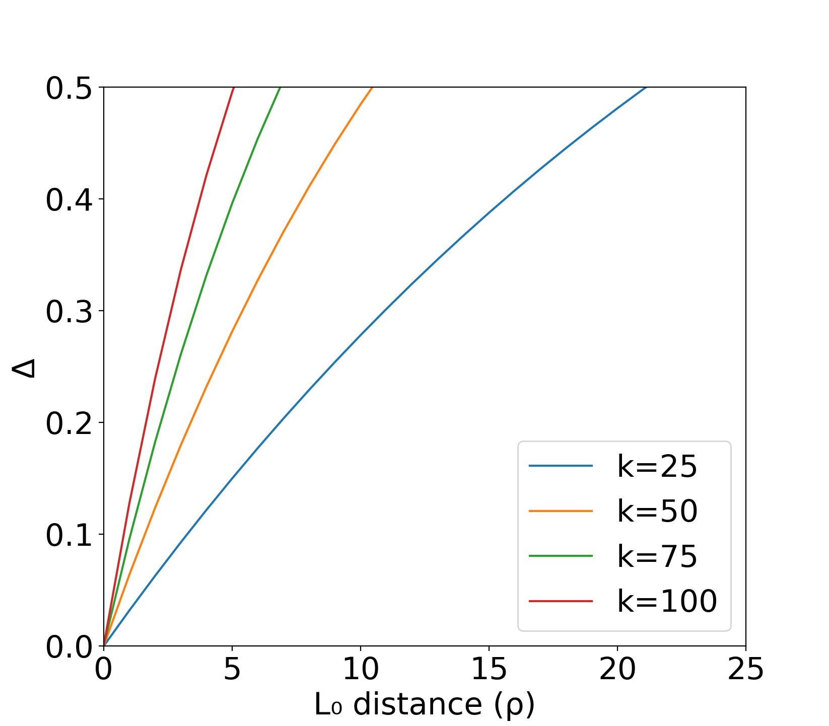
See Figure 2 for a plot of how the constant $\Delta$ scales with $k$ and $\rho$.

We present a short proof of Theorem 1 here:

In this section, we provide experimental results of the proposed method on MNIST, CIFAR-10, and ImageNet. When reporting results, we refer to the following quantities:

• •

  The certified robustness of a particular image ${\mathbf{x}}$ is the maximum $\rho$ for which we can certify (with probability at least $1-\alpha$) that the smoothed classifier $g({\mathbf{x}}^{\prime})$ will return the correct label where ${\mathbf{x}}^{\prime}$ is any adversarial perturbation of ${\mathbf{x}}$ such that $\|{\mathbf{x}}-{\mathbf{x}}^{\prime}\|_{0}\leq\rho$. If the unperturbed classification $g({\mathbf{x}})$ is itself incorrect, we define the certified robustness as N/A (Not Applicable).

• •

  The certified accuracy at $\rho$ on a dataset is the fraction of images in the dataset with certified robustness of at least $\rho$. In other words, it is the guaranteed accuracy of the classifier $g(.)$, if all images are corrupted with any $L_{0}$ adversarial attack of measure up to $\rho$.

• •

  The median certified robustness on a dataset is the median value of the certified robustness across the dataset. Equivalently, it is the maximum $\rho$ for which the certified accuracy at $\rho$ is at least $0.5$. When computing this median, images which $g(.)$ misclassifies when unperturbed (i.e., certified robustness is N/A) are counted as having $-\infty$ certified robustness. For example, if the robustness certificates of images in a dataset are {N/A,N/A,1,2,3}, the median certified robustness is 1, not 2.

• •

  The classification accuracy on a dataset is the fraction of images on which our empirical estimation of $g(.)$ returns the correct class label, and does not abstain.

• •

  The empirical adversarial attack magnitude of a particular image ${\mathbf{x}}$ is the minimum $\rho$ for which an adversarial attack can find an adversarial example ${\mathbf{x}}^{\prime}$ such that $\|{\mathbf{x}}-{\mathbf{x}}^{\prime}\|_{0}\leq\rho$, and such that our empirical classification procedure misclassifies or abstains on ${\mathbf{x}}^{\prime}$.

• •

  The median adversarial attack magnitude on a dataset is the median value of the empirical adversarial attack magnitude across the dataset.

Unless otherwise stated, the uncertainty $\alpha$ is 0.05, and 10,000 randomly-ablated samples are used to make each prediction. The empirical estimation procedure we use to generate certificates, from [\citeauthoryearCohen, Rosenfeld, and Kolter2019], requires two sampling steps: the first to identify the majority class $i$, and the second to bound $\underline{p_{i}({\mathbf{x}})}$. We use 1,000 and 10,000 samples, respectively, for these two steps.

In this paper, we introduced a novel smoothing-based certifiably robust classification method against sparse adversarial attacks, in which the adversary can perturb a certain number features in input samples. Our method, which is modeled after randomised smoothing methods for certifiably robust classification for $L_{1}$ and $L_{2}$ attack models, was shown to produce non-trivial robustness certificates on MNIST, CIFAR-10, and ImageNet, and to be an effective empirical defense against $L_{0}$ attacks on MNIST.

This work was supported in part by NSF award CDS&E:1854532 and award HR00111990077.

References

- [\citeauthoryearBafna, Murtagh, and Vyas2018] Bafna, M.; Murtagh, J.; and Vyas, N. 2018. Thwarting adversarial examples: An -robust sparse fourier transform. In Advances in Neural Information Processing Systems, 10075–10085.
- [\citeauthoryearCarlini and Wagner2016] Carlini, N., and Wagner, D. 2016. Defensive distillation is not robust to adversarial examples. arXiv preprint arXiv:1607.04311.
- [\citeauthoryearCarlini and Wagner2017] Carlini, N., and Wagner, D. 2017. Towards evaluating the robustness of neural networks. In 2017 38th IEEE Symposium on Security and Privacy (SP), 39–57. IEEE.
- [\citeauthoryearCohen, Rosenfeld, and Kolter2019] Cohen, J.; Rosenfeld, E.; and Kolter, Z. 2019. Certified adversarial robustness via randomized smoothing. In International Conference on Machine Learning, 1310–1320.
- [\citeauthoryearDong et al.2018] Dong, Y.; Liao, F.; Pang, T.; Su, H.; Zhu, J.; Hu, X.; and Li, J. 2018. Boosting adversarial attacks with momentum. In 2018 IEEE/CVF Conference on Computer Vision and Pattern Recognition, 9185–9193. IEEE.
- [\citeauthoryearGoodfellow, Shlens, and Szegedy2015] Goodfellow, I. J.; Shlens, J.; and Szegedy, C. 2015. Explaining and harnessing adversarial examples. In 3rd International Conference on Learning Representations, ICLR 2015, San Diego, CA, USA, May 7-9, 2015.
- [\citeauthoryearGowal et al.2018] Gowal, S.; Dvijotham, K.; Stanforth, R.; Bunel, R.; Qin, C.; Uesato, J.; Mann, T.; and Kohli, P. 2018. On the effectiveness of interval bound propagation for training verifiably robust models. arXiv preprint arXiv:1810.12715.
- [\citeauthoryearHe et al.2016] He, K.; Zhang, X.; Ren, S.; and Sun, J. 2016. Deep residual learning for image recognition. In Proceedings of the IEEE conference on computer vision and pattern recognition, 770–778.
- [\citeauthoryearHosseini, Kannan, and Poovendran2019] Hosseini, H.; Kannan, S.; and Poovendran, R. 2019. Dropping pixels for adversarial robustness. In Proceedings of the IEEE Conference on Computer Vision and Pattern Recognition Workshops, 0–0.
- [\citeauthoryearKurakin, Goodfellow, and Bengio2018] Kurakin, A.; Goodfellow, I. J.; and Bengio, S. 2018. Adversarial examples in the physical world. In Artificial Intelligence Safety and Security. Chapman and Hall/CRC. 99–112.
- [\citeauthoryearLecuyer et al.2019] Lecuyer, M.; Atlidakis, V.; Geambasu, R.; Hsu, D.; and Jana, S. 2019. Certified robustness to adversarial examples with differential privacy. In 2019 2019 IEEE Symposium on Security and Privacy (SP), 726–742. Los Alamitos, CA, USA: IEEE Computer Society.
- [\citeauthoryearLee et al.2019] Lee, G.-H.; Yuan, Y.; Chang, S.; and Jaakkola, T. S. 2019. Tight certificates of adversarial robustness for randomly smoothed classifiers. arXiv preprint arXiv:1906.04948.
- [\citeauthoryearLi et al.2018] Li, B.; Chen, C.; Wang, W.; and Carin, L. 2018. Second-order adversarial attack and certifiable robustness. arXiv preprint arXiv:1809.03113.
- [\citeauthoryearLiu2019] Liu, K. 2019. 95.16% on cifar10 with pytorch. https://github.com/kuangliu/pytorch-cifar.
- [\citeauthoryearMadry et al.2017] Madry, A.; Makelov, A.; Schmidt, L.; Tsipras, D.; and Vladu, A. 2017. Towards deep learning models resistant to adversarial attacks. arXiv preprint arXiv:1706.06083.
- [\citeauthoryearMeng and Chen2017] Meng, D., and Chen, H. 2017. Magnet: a two-pronged defense against adversarial examples. In Proceedings of the 2017 ACM SIGSAC Conference on Computer and Communications Security, 135–147. ACM.
- [\citeauthoryearPapernot et al.2016a] Papernot, N.; McDaniel, P.; Jha, S.; Fredrikson, M.; Celik, Z. B.; and Swami, A. 2016a. The limitations of deep learning in adversarial settings. In 2016 IEEE European Symposium on Security and Privacy (EuroS&P), 372–387. IEEE.
- [\citeauthoryearPapernot et al.2016b] Papernot, N.; McDaniel, P.; Wu, X.; Jha, S.; and Swami, A. 2016b. Distillation as a defense to adversarial perturbations against deep neural networks. In 2016 IEEE Symposium on Security and Privacy (SP), 582–597. IEEE.
- [\citeauthoryearPaszke et al.2017] Paszke, A.; Gross, S.; Chintala, S.; Chanan, G.; Yang, E.; DeVito, Z.; Lin, Z.; Desmaison, A.; Antiga, L.; and Lerer, A. 2017. Automatic differentiation in PyTorch. In NIPS Autodiff Workshop.
- [\citeauthoryearRauber, Brendel, and Bethge2017] Rauber, J.; Brendel, W.; and Bethge, M. 2017. Foolbox: A python toolbox to benchmark the robustness of machine learning models. arXiv preprint arXiv:1707.04131.
- [\citeauthoryearSalman et al.2019] Salman, H.; Yang, G.; Li, J.; Zhang, P.; Zhang, H.; Razenshteyn, I.; and Bubeck, S. 2019. Provably robust deep learning via adversarially trained smoothed classifiers. arXiv preprint arXiv:1906.04584.
- [\citeauthoryearSchott et al.2019] Schott, L.; Rauber, J.; Bethge, M.; and Brendel, W. 2019. Towards the first adversarially robust neural network model on mnist. In Seventh International Conference on Learning Representations (ICLR 2019), 1–16.
- [\citeauthoryearSzegedy et al.2013] Szegedy, C.; Zaremba, W.; Sutskever, I.; Bruna, J.; Erhan, D.; Goodfellow, I.; and Fergus, R. 2013. Intriguing properties of neural networks. arXiv preprint arXiv:1312.6199.
- [\citeauthoryearTsipras et al.2019] Tsipras, D.; Santurkar, S.; Engstrom, L.; Turner, A.; and Madry, A. 2019. Robustness may be at odds with accuracy. In 7th International Conference on Learning Representations, ICLR 2019, New Orleans, LA, USA, May 6-9, 2019.
- [\citeauthoryearWong and Kolter2018] Wong, E., and Kolter, Z. 2018. Provable defenses against adversarial examples via the convex outer adversarial polytope. In International Conference on Machine Learning, 5283–5292.
- [\citeauthoryearXu, Evans, and Qi2017] Xu, W.; Evans, D.; and Qi, Y. 2017. Feature squeezing: Detecting adversarial examples in deep neural networks. arXiv preprint arXiv:1704.01155.
- [\citeauthoryearZhang et al.2017] Zhang, C.; Bengio, S.; Hardt, M.; Recht, B.; and Vinyals, O. 2017. Understanding deep learning requires rethinking generalization. In 5th International Conference on Learning Representations, ICLR 2017, Toulon, France, April 24-26, 2017, Conference Track Proceedings.
Appendix A Architecture and Training Parameters for MNIST