Multi-group Multicast Beamforming: Optimal Structure and Efficient Algorithms

Min Dong Thanks: The authors are with the Department of Electrical, Computer and Software Engineering, Ontario Tech University, Ontario L1G 0C5, Canada. Email: {min.dong, qiqi.wang}@ontariotechu.ca. Part of this work was presented in [1]. Qiqi Wang

Abstract

This paper considers the multi-group multicast beamforming optimization problem, for which the optimal solution has been unknown due to the non-convex and NP-hard nature of the problem. By utilizing the successive convex approximation numerical method and Lagrangian duality, we obtain the optimal multicast beamforming solution structure for both the quality-of-service (QoS) problem and the max-min fair (MMF) problem. The optimal structure brings valuable insights into multicast beamforming: We show that the notion of uplink-downlink duality can be generalized to the multicast beamforming problem. The optimal multicast beamformer is a weighted MMSE filter based on a group-channel direction: a generalized version of the optimal downlink multi-user unicast beamformer. We also show that there is an inherent low-dimensional structure in the optimal multicast beamforming solution independent of the number of transmit antennas, leading to efficient numerical algorithm design, especially for systems with large antenna arrays. We propose efficient algorithms to compute the multicast beamformer based on the optimal beamforming structure. Through asymptotic analysis, we characterize the asymptotic behavior of the multicast beamformers as the number of antennas grows, and in turn, provide simple closed-form approximate multicast beamformers for both the QoS and MMF problems. This approximation offers practical multicast beamforming solutions with a near-optimal performance at very low computational complexity for large-scale antenna systems.

Index Terms:

Multicast beamforming, optimal solution structure, duality, large-scale antenna systems, computational complexity, asymptotic beamforming

I Introduction

We consider the downlink multi-group multicast beamforming problem. In wireless communications, common data may be intended for a group of users. Multi-antenna multicast beamforming is an efficient physical-layer transmission technique to deliver common data to multiple users simultaneously, improving both spectrum and power efficiency. Multicast transmit beamforming has been first considered more than a decade ago [2]. The attention to this technique is fast rising in recent years for its potential to support wireless multicasting and content distribution in the growing number of wireless services and applications (e.g., video conference, mobile commerce, intelligent transportation systems). Besides these, in the emerging cache-aided wireless networking technologies, (coded) multicasting is utilized in coded caching techniques for content delivery of individual data requests to reduce wireless traffic [3]. This new area of application further expands the potential of multicast beamforming techniques in improving content distribution and delivery in the rising trend of content-centric wireless networks.

The problem of multicast beamforming optimization has initially been considered for a single user group [2, 4, 5]. It has later been extended to multiple user groups [6, 7, 8] and multi-cell networks [9, 10], where inter-group or inter-cell interference further complicates the problem. Two types of problem formulation are typically considered for multicast beamforming: the transmit power minimization subject to a minimum signal-to-interference-and-noise (SINR) target for each user – the quality of service (QoS) problem, and the maximization of (weighted) minimum SINR of all users subject to a total transmit power budget – the max-min fair (MMF) problem. The family of these multicast beamforming problems are non-convex and are shown to be NP-hard in general [2]. Existing literature works have focused on developing numerical algorithms or signal processing methods to obtain feasible solutions with good performance. It is more direct to solve the QoS problem than the MMF problem, although the feasibility of the QoS problem imposes challenges in designing numerical methods. The MMF problem is typically handled in the literature works by iteratively solving the QoS problem.

Among existing methods for tackling the multicast beamforming problems, semi-definite relaxation (SDR) is a popular numerical approach to obtain an approximate (sometimes global optimal) solution by relaxing the problem into a semi-definite problem (SDP) to solve [2, 4, 6, 11, 10]. Its provable approximation accuracies are shown via theoretical analysis [12]. However, as the problem size increases, the computational complexity of SDR-based methods grows quickly, and the performance deteriorates noticeably [6]. These drawbacks make the direct use of this approach unsuitable for future large-scale wireless systems, in particular for massive multiple-input and multiple-output (MIMO) systems with large-scale antenna arrays [13]¹¹ 1 The computational complexity to solve the QoS problem directly via SDR is ${\cal O}(N^{6})$ where $N$ is the number of antennas at the base station.. For addressing these issues, the successive convex approximation (SCA) [14] has been proposed for multicast beamforming in large-scale systems [15, 16, 17]. The SCA is an iterative numerical method to solve the original problem through a sequence of convex approximations. Although it shows good performance with reduced complexity, the SCA requires an initial feasible solution for the problem that is generally difficult to obtain. Besides, its computational complexity is still high for a large number of antennas. There is an increasing need for effective and efficient multicast beamforming design. To further address the computational complexity, low-complexity multicast beamforming schemes have recently been proposed for massive MIMO systems for multi-group [18, 19] and multi-cell [20, 21] scenarios. These schemes use specific beamforming strategies (e.g., maximum ratio transmission (MRT) or zero-forcing (ZF)) in combination with SCA or distributed optimization techniques to reduce complexity.

A primary challenge for the multicast beamforming problems is the elusive optimal solution structure. Prevailing numerical optimization methods target at finding good feasible solutions to the non-convex problems. However, theoretically, they are unable to characterize or offer a fundamental understanding of the beamforming structure for multicasting, and practically, they face challenges in both computational complexity and performance for large-scale systems. In this paper, in the general multi-group setting, we characterize the optimal multicast beamforming structure for both QoS and MMF problems. We take a different approach from existing works by exploring both the numerical method of iterative approximation via SCA and Lagrangian duality and combining the two techniques to obtain the optimal multicast beamforming solution structure for the QoS problem. This solution structure provides valuable insights into the optimal multicast beamforming: We establish an uplink-downlink duality interpretation for downlink multicast beamforming, as a generalization of the uplink-downlink duality for downlink multi-user unicast beamforming. We show that the optimal beamforming solution for a multicast group has an intuitive structure: a weighted minimum mean square error (MMSE) filter, formed by the group-channel direction and the noise plus weighted channel covariance matrix. This optimal multicast beamforming is a generalized version of the optimal downlink multi-user unicast beamforming. We draw connections and explain differences between the multicast and unicast beamforming. An important finding from the optimal structure is that the optimal multicast beamforming has an inherent low-dimensional structure, where only weights of user channels in the group need to be computed. This structure changes the dimension of the multicast beamforming problem from the number of antennas to the number of users per group, and the problem size may be further reduced depending on the dimension of the subspace spanned by the user channels in each group. This optimal multicast beamforming structure gives rise to efficient numerical methods to compute the beamforming solution, especially for massive MIMO systems with large-scale antenna arrays.

With the optimal multicast beamforming structure, we only need to compute the parameters in the optimal solution. Due to the NP-hard nature of the original problem, obtaining their optimal values are difficult. We propose efficient numerical algorithms to compute these parameters, including Lagrange multipliers (associated with the SINR constraints) and user weights (in the group-channel direction). Our algorithm for computing the Lagrange multipliers is asymptotically optimal. We derive the asymptotic expression of the multipliers. It can be used directly for systems with a large number of antennas, further eliminating the computational need. To compute the weights, we transform the original problem into a weight optimization problem of a much smaller size, independent of the number of antennas. Taking advantage of this small problem size, we apply the SDR or SCA method for good approximate or locally optimal solutions with very low computational complexity.

We extend our results to the MMF problem. Exploring the inverse relation of the QoS and MMF problems, we directly obtain the optimal MMF multicast beamforming structure. Computing the MMF beamformers is more involved, which requires iteratively computing the QoS beamformers. However, we show that the asymptotic results obtained from the QoS problem lead to simple asymptotic MMF beamformers, including a closed-form asymptotic beamformer. They provide simple approximate multicast beamforming solutions for a large number of antennas. Simulation demonstrates both the computational efficiency and the near-optimal performance by our proposed algorithms using the optimal multicast beamforming structure.

I-A Related Work

Downlink multicast transmit beamforming has been studied for both QoS and MMF problems in single-group [2, 5, 22, 4, 23] and multi-group [6, 7, 8] settings, as well as in multi-cell scenarios [9, 10]. It has also been considered in other network scenarios, such as relay networks [24, 25], cognitive spectrum access [26], and cache-aided cloud radio access networks [27]. The family of problems are non-convex quadratically constrained quadratic programming (QCQP) problems and are shown to be NP-hard in general [2]. The SDR approach was proposed [2] and has been widely used [4, 6, 10, 8], due to its bounded approximation performance [12] and can be efficiently solved by interior-point methods with polynomial time complexity [28] for problems with a moderately small size. Different techniques have been proposed to extract a rank-one approximate solution to the original problem from the relaxed problem, including randomization methods [2, 4] and rank-reduction methods [29]. The conditions for the existence of an optimal rank-one solution for the SDR problem were also investigated [29]. Rank-two multicasting beamforming techniques were also proposed as a generalization of the rank-one SDR-based approach by combining beamforming and the Alamouti space-time code [4, 22]. Alternative signaling processing approaches, such as channel orthogonalization, were also proposed [5, 23].

Recently, a great deal of effort has been made in developing computationally efficient numerical methods for massive MIMO systems with large-scale antenna arrays [15, 30, 16, 18, 19, 17, 20, 21]. The SCA method is applied to find a stationary solution for single-group [15], multi-group [16], and multi-cell [17] scenarios. It is shown to perform better than SDR-based methods in large-scale systems with reduced computational complexities. However, the SCA method requires a feasible initial point that is difficult to obtain in general. Several optimization techniques have been developed to improve SCA-type methods [31, 17]. For massive MIMO systems, the existing SCA-based methods are still computationally intensive. Asymptotic multicast beamformers were derived by invoking channel orthogonality at the asymptotic regime to eliminate interference [30, 32]. While they have simple analytical expressions, it is observed that these beamformers perform poorly in most practical systems [32, 20]. We will explain this phenomenon of slow convergence to asymptotic orthogonality in Section IV-B through our asymptotic analysis. Several low-complexity methods have been proposed for massive MIMO systems. These include a two-layer method combining ZF and SCA [18] and an alternating direction method of multipliers (ADMM) algorithm [19] for multi-group multicasting, and a weighted MRT beamforming method for both centralized and distributed coordinated multicast beamforming in multi-cell scenarios [20, 21].

Besides the above, multicast beamforming in overloaded systems with fewer antennas than the users has also been investigated recently. With insufficient degrees of freedom, the rate-splitting based MMF beamforming strategies have been proposed for single-carrier or multi-carrier systems [33, 34, 35]. Multicast beamforming using other design objectives has also been considered, such as energy efficiency maximization [35, 36] and the sum-rate maximization in a mixed multicast and broadcast scenario [37].

I-B Organization and Notations

The rest of this paper is organized as follows. In Section II, we present the system model and problem formulation for multi-group multicast beamforming. In Section III, we derive our main result of the optimal multicast beamforming in semi-closed-form for the QoS problem and characterize the solution structure. In Section IV, numerical algorithms are proposed for computing the parameters in the optimal solution, and asymptotic analysis is provided at the large-scale antenna array regime. In Section V, we describe the optimal solution structure for the MMF problem, its relation to the solution structure for the QoS problem, and the asymptotic MMF beamforming solution. Simulation results are presented in Section VI, and the conclusion and possible extension are provided in Section VII.

Notations: Hermitian, transpose, and conjugate are denoted as $(\cdot)^{H}$ , $(\cdot)^{T}$ , and $(\cdot)^{*}$ , respectively. The Euclidean norm of a vector is denoted by $\left\|\cdot\right\|$ . The notation ${\bf a}\succcurlyeq{\bf 0}$ means element-wise non-negative, and ${\bf A}\succcurlyeq 0$ indicates matrix ${\bf A}$ being positive semi-definite. The trace of matrix ${\bf A}$ is denoted as ${\rm tr}({\bf A})$ . The real part of $x$ is denoted by $\operatorname{\mathfrak{Re}}\{x\}$ , and $E(x)$ denotes the expectation of $x$ . The abbreviation i.i.d. stands for independent and identically distributed, and ${\bf x}\sim{\cal C}{\cal N}({\bf 0},{\bf I})$ means ${\bf x}$ is a complex Gaussian random vector with zero mean and covariance ${\bf I}$ .

II System Model and Problem Formulation

Consider a downlink multi-group multicasting scenario, where a BS equipped with $N$ antennas serves $G$ multicast groups, sending each group a common message that is independent of other groups. Let ${\cal G}=\{1,\ldots,G\}$ denote the set of group indices. Each group $i$ consists of $K_{i}$ single-antenna users, and the set of user indices in the group is denoted by ${\cal K}_{i}=\{1,\ldots,K_{i}\}$ , $i\in{\cal G}$ . User groups are disjoint, i.e., each user only belongs to one multicast group and only receives the multicast message intended to this group. The total number of users in all groups is denoted by $K_{\text{tot}}\triangleq\sum_{i=1}^{G}K_{i}$ .

Let ${\bf h}_{ik}$ denote the $N\times 1$ channel vector between the BS and user $k$ in group $i$ , and let ${\bf w}_{i}$ denote the $N\times 1$ multicast beamforming vector for group $i\in{\cal G}$ . The received signal at user $k$ in group $i$ is given by

\displaystyle y_{ik}={\bf w}_{i}^{H}{\bf h}_{ik}s_{i}+\sum_{j\neq i}{\bf w}_{j}^{H}{\bf h}_{ik}s_{j}+n_{ik}

(1)

where $s_{i}$ is the data symbol intended for group $i$ with unit power $E(|s_{i}|^{2})=1$ , and $n_{ik}$ is the receiver additive white Gaussian noise with zero mean and variance $\sigma^{2}$ . The transmit power at the BS is given by $\sum_{i=1}^{G}\|{\bf w}_{i}\|^{2}$ . The received SINR at user $k$ in group $i$ is given by

\displaystyle\textrm{SINR}_{ik}

\displaystyle=\displaystyle\frac{|{\bf w}_{i}^{H}{\bf h}_{ik}|^{2}}{\displaystyle\sum_{j\neq i}|{\bf w}_{j}^{H}{\bf h}_{ik}|^{2}+\sigma^{2}}.

(2)

Depending on the design focus, two problem formulations are typically considered for the multicast beamforming: 1) the QoS problem for transmit power minimization while meeting the received SINR target at each user, formulated as

	$\displaystyle{\cal P}_{o}:\ \min_{{\bf w}}$	$\displaystyle\ \ \sum_{i=1}^{G}\\|{\bf w}_{i}\\|^{2}$
	subject to	$\displaystyle\ \ \textrm{SINR}_{ik}\geq\gamma_{ik},\ k\in{\cal K}_{i},~i\in{\cal G}$		(3)

where ${\bf w}\triangleq[{\bf w}_{1}^{H},\ldots,{\bf w}_{G}^{H}]^{H}$ , and $\gamma_{ik}$ is the SINR target at user $k$ in group $i$ . 2) The (weighted) MMF problem for maximizing the minimum (weighted) SINR, subject to the transmit power constraint, formulated as

	$\displaystyle{\cal S}_{o}:\ \max_{{\bf w}}\min_{i,k}$	$\displaystyle\ \ \frac{\textrm{SINR}_{ik}}{\gamma_{ik}}$
	subject to	$\displaystyle\ \ \sum_{i=1}^{G}\\|{\bf w}_{i}\\|^{2}\leq P$

where $P$ is the transmit power budget, and $\{\gamma_{ik}\}$ here serve as the weights to control the fairness or service grades among users.

Remark (Feasibility): The QoS problem ${\cal P}_{o}$ for multi-group multicast beamforming may not always be feasible, depending on the channels $\{{\bf h}_{ik}\}$ and the SINR targets $\{\gamma_{ik}\}$ . On the other hand, the MMF problem ${\cal S}_{o}$ is always feasible, but more involved than the QoS problem to solve. In the following sections, we assume the QoS problem ${\cal P}_{o}$ being feasible to derive the optimal multicast beamformer structure.

III Optimal Multicast Beamforming Structure

We now focus on the multicast beamforming QoS problem ${\cal P}_{o}$ , which is known to be a non-convex QCQP problem and NP-hard. The optimal solution is difficult to obtain either in the primal domain, or in the dual domain due to the unknown duality gap. In the following, we take a different approach by exploring the problem via the SCA method and derive the structure of the optimal solution.

III-A The SCA Method

The SCA method is a numerical approximation method that iteratively solves a non-convex optimization problem via a sequence of convex approximations of the original problem, provided that an initial feasible point is given. For non-convex problems with a convex objective function, the SCA method is proven to converge to a stationary solution [14]. The SCA method, and in particular, the convex-concave procedure (CCP) as a special case, has been applied to find a feasible multicast beamforming solution in several existing works [15, 16, 17, 18]. The SCA method is briefly described below.

Consider $N\times 1$ auxiliary vector ${\bf z}_{i}$ , $i\in{\cal G}$ . For matrix ${\bf A}\succcurlyeq{\bf 0}$ , we have $({\bf w}_{i}-{\bf z}_{i})^{H}{\bf A}({\bf w}_{i}-{\bf z}_{i})\geq 0$ , for any ${\bf z}_{i}$ . It follows that ${\bf w}_{i}^{H}{\bf A}{\bf w}_{i}\geq 2\operatorname{\mathfrak{Re}}\{{\bf w}_{i}^{H}{\bf A}{\bf z}_{i}\}-{\bf z}_{i}^{H}{\bf A}{\bf z}_{i}$ . Denote ${\bf z}\triangleq[{\bf z}_{1}^{H},\ldots,{\bf z}_{G}^{H}]^{H}$ . Given ${\bf z}$ , applying the above inequality to SINR constraint (3), we obtain the following optimization problem which is a convex approximation of ${\cal P}_{o}$

$\displaystyle\hskip-1.99997pt{\cal P}_{\text{\tiny SCA}}({\bf z}):\min_{{\bf w}}$	$\displaystyle\ \sum_{i=1}^{G}\\|{\bf w}_{i}\\|^{2}$
subject to	$\displaystyle\ \gamma_{ik}\sum_{j\neq i}\|{\bf w}_{j}^{H}{\bf h}_{ik}\|^{2}-2\operatorname{\mathfrak{Re}}\{{\bf w}_{i}^{H}{\bf h}_{ik}{\bf h}_{ik}^{H}{\bf z}_{i}\}$
	$\displaystyle\ \ +\|{\bf z}_{i}^{H}{\bf h}_{ik}\|^{2}\leq-\gamma_{ik}\sigma^{2},\ k\in{\cal K}_{i},i\in{\cal G}.$	(4)

With non-convex SINR constraint (3) being replaced by convex constraint (4), problem ${\cal P}_{\text{\tiny SCA}}({\bf z})$ is now convex. The main steps in the SCA method are summarized below:

1.

Set initial feasible point ${\bf z}^{(0)}$ ; Set $l=0$ .
2.

Solve ${\cal P}_{\text{\tiny SCA}}({\bf z}^{(l)})$ and obtain the optimal solution ${\bf w}^{\star}({\bf z}^{(l)})$ .
3.

Set ${\bf z}^{(l+1)}={\bf w}^{\star}({\bf z}^{(l)})$ .
4.

Set $l\leftarrow l+1$ . Repeat Steps 2-4 until convergence.

The above SCA method is guaranteed to converge to a stationary point ${\bf w}^{\star}$ of ${\cal P}_{o}$ [14]. Since the global optimal solution is a stationary point, the above procedure may converge to the global optimal solution ${\bf w}^{o}$ of ${\cal P}_{o}$ , provided that the initial point ${\bf z}^{(0)}$ is appropriately chosen, e.g., ${\bf z}^{(0)}$ is at the vicinity of ${\bf w}^{o}$ . When this is the case, we have ${\bf z}^{(l)}\to{\bf w}^{\star}={\bf w}^{o}$ .

Remark: A challenge to use the SCA method for ${\cal P}_{o}$ is finding an initial feasible point ${\bf z}^{(0)}$ that satisfies the SINR constraint (3). Some existing works propose different methods to address this issue. Here, we focus on deriving the optimal solution structure via the SCA method, not the implementation or numerical behavior of this method. Thus, we only assume a feasible initial point ${\bf z}^{(0)}$ without discussing how to obtain it.

III-B The Optimal Multicast Beamforming Solution

Since ${\cal P}_{\text{\tiny SCA}}({\bf z})$ is convex (and Slater’s condition holds), we obtain its optimal solution from its Lagrange dual domain. The Lagrangian for ${\cal P}_{\text{\tiny SCA}}({\bf z})$ is given by

	$\displaystyle\hskip-5.0pt{\cal L}({\bf z},{\bf w},\boldsymbol{\lambda})=$	$\displaystyle\sum_{i=1}^{G}\\|{\bf w}_{i}\\|^{2}+\sum_{i=1}^{G}\sum_{k=1}^{K_{i}}\lambda_{ik}\bigg[\gamma_{ik}\sum_{j\neq i}\left\|{{\bf w}_{j}^{H}{\bf h}_{ik}}\right\|^{2}$
		$\displaystyle\!\!\!-2\mathfrak{Re}\left\{{\bf w}_{i}^{H}{\bf h}_{ik}{\bf h}_{ik}^{H}{\bf z}_{i}\right\}+\left\|{\bf z}_{i}^{H}{\bf h}_{ik}\right\|^{2}\!+\sigma^{2}\gamma_{ik}\bigg]$		(5)

where $\lambda_{ik}$ is the Lagrange multiplier associated with constraint (4) for user $k$ in group $i$ , and $\boldsymbol{\lambda}\triangleq[\boldsymbol{\lambda}_{1}^{T},\ldots,\boldsymbol{\lambda}_{G}^{T}]^{T}$ with $\boldsymbol{\lambda}_{i}\triangleq[\lambda_{i1},\ldots,\lambda_{iK_{i}}]^{T}$ . The Lagrange dual problem for ${\cal P}_{\text{\tiny SCA}}({\bf z})$ is given by

\displaystyle{{\cal D}_{\text{\tiny SCA}}({\bf z}):}\ \max_{\boldsymbol{\lambda}}

\displaystyle\ g({\bf z},\boldsymbol{\lambda})\quad\text{subject~to~}\ \boldsymbol{\lambda}\succcurlyeq{\bf 0}

where

\displaystyle g({\bf z},\boldsymbol{\lambda})\triangleq\min_{{\bf w}}\

\displaystyle{\cal L}({\bf z},{\bf w},\boldsymbol{\lambda}).

(6)

Regrouping the different terms in (5), the Lagrangian can be rewritten as

$\displaystyle{\cal L}({\bf z},{\bf w},\boldsymbol{\lambda})=$	$\displaystyle\sum_{i=1}^{G}\sum_{k=1}^{K_{i}}\lambda_{ik}\left(\sigma^{2}\gamma_{ik}+\left\|{\bf z}_{i}^{H}{\bf h}_{ik}\right\|^{2}\right)$
	$\displaystyle+\sum_{i=1}^{G}{\bf w}_{i}^{H}\left({\bf I}+\sum_{j\neq i}\sum_{k=1}^{K_{j}}\gamma_{jk}\lambda_{jk}{\bf h}_{jk}{\bf h}_{jk}^{H}\right){\bf w}_{i}$
	$\displaystyle-\sum_{i=1}^{G}2\operatorname{\mathfrak{Re}}\left\{{\bf z}_{i}^{H}\left(\sum_{k=1}^{K_{i}}\lambda_{ik}{\bf h}_{ik}{\bf h}_{ik}^{H}\right){\bf w}_{i}\right\}.$	(7)

Define $\boldsymbol{\nu}_{i}\triangleq\left(\sum_{k=1}^{K_{i}}\lambda_{ik}{\bf h}_{ik}{\bf h}_{ik}^{H}\right){\bf z}_{i}$ , and

\displaystyle{\bf R}_{i^{-}}(\boldsymbol{\lambda})

\displaystyle\triangleq{\bf I}+\sum_{j\neq i}\sum_{k=1}^{K_{j}}\lambda_{jk}\gamma_{jk}{\bf h}_{jk}{\bf h}_{jk}^{H}.

(8)

Then, the optimization problem (6) is equivalent to

\displaystyle\min_{{\bf w}}\sum_{i=1}^{G}\left({\bf w}_{i}^{H}{\bf R}_{i^{-}}(\boldsymbol{\lambda}){\bf w}_{i}-2\operatorname{\mathfrak{Re}}\left\{\boldsymbol{\nu}_{i}^{H}{\bf w}_{i}\right\}\right).

(9)

The above optimization problem can be decomposed into subproblems with respect to (w.r.t.) each ${\bf w}_{i}$ , $i\in{\cal G}$ , as

\displaystyle\min_{{\bf w}_{i}}\ {\bf w}_{i}^{H}{\bf R}_{i^{-}}(\boldsymbol{\lambda}){\bf w}_{i}-2\operatorname{\mathfrak{Re}}\{\boldsymbol{\nu}_{i}^{H}{\bf w}_{i}\},

(10)

and solved separately. Since the optimization problem (10) is convex, we can obtain its optimal solution in closed-form using KKT conditions [28]. The solution is given as follows.

Proposition 1.

The optimal solution for ${\cal P}_{\text{\tiny SCA}}({\bf z})$ is given by

\displaystyle{\bf w}_{i}^{\star}({\bf z})

\displaystyle={\bf R}_{i^{-}}^{-1}(\boldsymbol{\lambda}^{\star})\left(\sum_{k=1}^{K_{i}}\alpha_{ik}^{\star}{\bf h}_{ik}\right),\ \ i\in{\cal G}

(11)

where $\boldsymbol{\lambda}^{\star}$ is the optimal dual solution for ${\cal D}_{\text{\tiny SCA}}({\bf z})$ , and $\alpha_{ik}^{\star}\triangleq\lambda_{ik}^{\star}{\bf h}_{ik}^{H}{\bf z}_{i}$ , $k\in{\cal K}_{i}$ , $i\in{\cal G}$ .

Proof:

We first provide the complex gradients of two functions. Denote the real and imaginary part of vector ${\bf x}$ as ${\bf x}={\bf x}_{\textrm{R}}+j{\bf x}_{\textrm{I}}$ . For complex vector ${\bf c}$ , by the complex derivative operation [38], we have

	$\displaystyle\nabla{{\bf x}}\operatorname{\mathfrak{Re}}\{{\bf c}^{H}{\bf x}\}$	$\displaystyle=\frac{1}{2}\left(\nabla{{\bf x}_{\textrm{R}}}\operatorname{\mathfrak{Re}}\{{\bf c}^{H}{\bf x}\}-\rm{j}\nabla{{\bf x}_{\textrm{I}}}\operatorname{\mathfrak{Re}}\{{\bf c}^{H}{\bf x}\}\right)$
		$\displaystyle=\frac{1}{2}({\bf c}_{\textrm{R}}-\rm{j}{\bf c}_{\textrm{I}})=\frac{1}{2}{\bf c}^{*}$		(12)

where we note that $\operatorname{\mathfrak{Re}}\{{\bf c}^{H}{\bf x}\}={\bf c}_{\textrm{R}}^{T}{\bf x}_{\textrm{R}}+{\bf c}_{\textrm{I}}^{T}{\bf x}_{\textrm{I}}$ . Also, for Hermitian matrix ${\bf C}$ , we have

\displaystyle\nabla{\bf x}({\bf x}^{H}{\bf C}{\bf x})=({\bf C}{\bf x})^{*}.

(13)

The optimization problem (10) is an unconstrained convex optimization problem. Denote the objective function in (10) by $J({\bf z}_{i},{\bf w}_{i})$ for given ${\bf z}_{i}$ . Let $\boldsymbol{\lambda}^{\star}$ be the optimal Lagrange multiplier vector for the dual problem ${\cal D}_{\text{\tiny SCA}}({\bf z})$ . By the KKT condition, and from (12) and (13), at the optimality of ${\cal P}_{\text{\tiny SCA}}({\bf z})$ , the gradient of $J({\bf z}_{i},{\bf w}_{i})$ w.r.t. ${\bf w}_{i}$ satisfies

\displaystyle\nabla{{\bf w}_{i}}J({\bf z}_{i},{\bf w}_{i})=\left({\bf R}_{i^{-}}(\boldsymbol{\lambda}^{\star}){\bf w}_{i}({\bf z})\right)^{*}-\boldsymbol{\nu}_{i}^{*}={\bf 0},

(14)

and we obtain

	$\displaystyle\hskip-5.0pt{\bf w}_{i}^{\star}({\bf z})$	$\displaystyle={\bf R}_{i^{-}}^{-1}(\boldsymbol{\lambda}^{\star})\boldsymbol{\nu}_{i}={\bf R}_{i^{-}}^{-1}(\boldsymbol{\lambda}^{\star})\left(\sum_{k=1}^{K_{i}}\lambda_{ik}^{\star}{\bf h}_{ik}{\bf h}_{ik}^{H}\right){\bf z}_{i}$		(15)
		$\displaystyle={\bf R}_{i^{-}}^{-1}(\boldsymbol{\lambda}^{\star})\left(\sum_{k=1}^{K_{i}}\alpha_{ik}^{\star}{\bf h}_{ik}\right)$		(16)

where $\alpha_{ik}^{\star}\triangleq\lambda_{ik}^{\star}{\bf h}_{ik}^{H}{\bf z}_{i}$ , for $k\in{\cal K}_{i}$ , $i\in{\cal G}$ . ∎

Examining the optimal solution ${\bf w}_{i}^{\star}({\bf z})$ in Proposition 1, we note that the dependency of ${\bf w}_{i}^{\star}({\bf z})$ on ${\bf z}$ is only through $\boldsymbol{\lambda}^{\star}$ in ${\bf R}_{i^{-}}(\boldsymbol{\lambda}^{\star})$ and $\{\alpha_{ik}^{\star}\}$ , both of which are functions of ${\bf z}$ . This implies that, as the SCA method iteratively updates ${\bf z}$ , the optimal solution ${\bf w}^{\star}({\bf z})$ for ${\cal P}_{\text{\tiny SCA}}({\bf z})$ is updated accordingly, but only through $\boldsymbol{\lambda}^{\star}$ and $\{\alpha_{ik}^{\star}\}$ , while the structure of ${\bf w}^{\star}({\bf z})$ is unchanged. Thus, if ${\bf z}\to{\bf w}^{o}$ , then the optimal solution for ${\cal P}_{o}$ is obtained.

Define ${\bf H}_{i}\triangleq[{\bf h}_{i1},\ldots,{\bf h}_{iK_{i}}]$ as the channel matrix for group $i$ , and

\displaystyle{\bf R}(\boldsymbol{\lambda})

\displaystyle\triangleq{\bf I}+\sum_{i=1}^{G}\sum_{k=1}^{K_{i}}\lambda_{ik}\gamma_{ik}{\bf h}_{ik}{\bf h}_{ik}^{H}.

(17)

We state the main result in the following theorem.

Theorem 1.

The optimal beamforming solution for the multi-group multicast beamforming QoS problem ${\cal P}_{o}$ is given by

\displaystyle{\bf w}_{i}^{o}={\bf R}^{-1}(\boldsymbol{\lambda}^{o})\sum_{k=1}^{K_{i}}a_{ik}^{o}{\bf h}_{ik}={\bf R}^{-1}(\boldsymbol{\lambda}^{o}){\bf H}_{i}{\bf a}_{i}^{o},\ i\in{\cal G}

(18)

where $\boldsymbol{\lambda}^{o}$ is the optimal dual solution for ${\cal D}_{\text{\tiny SCA}}({\bf w}^{o})$ , $a_{ik}^{o}\triangleq\lambda_{ik}^{o}\delta_{ik}(1+\gamma_{ik})$ with $\delta_{ik}\triangleq{\bf h}_{ik}^{H}{\bf w}_{i}^{o}$ , $k\in{\cal K}_{i}$ , and ${\bf a}_{i}^{o}\triangleq[a_{i1}^{o},\ldots,a_{iK_{i}}^{o}]^{T}$ , $i\in{\cal G}$ .

Proof:

The SCA iterative procedure described in Section III-A is guaranteed to converge to a stationary point. This means that assuming initial ${\bf z}^{(0)}$ chosen at the vicinity of the global optimal solution, the method will converge to the global optimal solution, i.e., ${\bf z}\to{\bf w}^{o}$ , and ${\bf w}_{i}^{\star}({\bf z})\to{\bf w}_{i}^{o}$ . Specifically, from (15), the optimal ${\bf w}_{i}^{\star}({\bf z})$ for ${\cal P}_{\text{\tiny SCA}}({\bf z})$ in each iteration satisfies

\displaystyle{\bf R}_{i^{-}}(\boldsymbol{\lambda}^{\star}){\bf w}_{i}^{\star}({\bf z})

\displaystyle=\sum_{k=1}^{K_{i}}\lambda_{ik}^{\star}{\bf h}_{ik}\left({\bf h}_{ik}^{H}{\bf z}_{i}\right).

(19)

From (17), we have ${\bf R}_{i^{-}}(\boldsymbol{\lambda})={\bf R}(\boldsymbol{\lambda})-\sum_{k=1}^{K_{i}}\lambda_{ik}\gamma_{ik}{\bf h}_{ik}{\bf h}_{ik}^{H}$ . Substituting this into (19), we have

\displaystyle{\bf R}(\boldsymbol{\lambda}^{\star}){\bf w}_{i}^{\star}({\bf z})

\displaystyle=\sum_{k=1}^{K_{i}}\lambda_{ik}^{\star}\left({\bf h}_{ik}^{H}{\bf z}_{i}+\gamma_{ik}{\bf h}_{ik}^{H}{\bf w}_{i}^{\star}({\bf z})\right){\bf h}_{ik}.

(20)

At the convergence ${\bf z}\to{\bf w}^{o}$ , we have ${\bf h}_{ik}^{H}{\bf z}_{i}\to{\bf h}_{ik}^{H}{\bf w}_{i}^{o}\triangleq\delta_{ik}$ . Also, as ${\bf z}\to{\bf w}^{o}$ , we have ${\bf w}_{i}^{\star}({\bf z})\to{\bf w}_{i}^{o}$ , and the optimal $\boldsymbol{\lambda}^{\star}$ for ${\cal D}_{\text{\tiny SCA}}({\bf z})$ converges to $\boldsymbol{\lambda}^{o}$ for ${\cal D}_{\text{\tiny SCA}}({\bf w}^{o})$ . Then, the expression in (20) becomes

\displaystyle{\bf R}(\boldsymbol{\lambda}^{o}){\bf w}_{i}^{o}

\displaystyle=\sum_{k=1}^{K_{i}}\lambda_{ik}^{o}\delta_{ik}(1+\gamma_{ik}){\bf h}_{ik},

(21)

and thus we have

\displaystyle{\bf w}_{i}^{o}

\displaystyle={\bf R}^{-1}(\boldsymbol{\lambda}^{o})\!\!\sum_{k=1}^{K_{i}}\lambda_{ik}^{o}\delta_{ik}(1+\gamma_{ik}){\bf h}_{ik}={\bf R}^{-1}(\boldsymbol{\lambda}^{o})\!\!\sum_{k=1}^{K_{i}}a_{ik}^{o}{\bf h}_{ik}

where $a_{ik}^{o}\triangleq\lambda_{ik}^{o}\delta_{ik}(1+\gamma_{ik})$ , for $k\in{\cal K}_{i}$ , $i\in{\cal G}$ . ∎

Theorem 1 presents the structure of the optimal multicast beamforming vector ${\bf w}_{i}^{o}$ for ${\cal P}_{o}$ . The optimal solution ${\bf w}_{i}^{o}$ in (18) is expressed in semi-closed-form, where $\boldsymbol{\lambda}^{o}$ and ${\bf a}_{i}^{o}$ need to be determined numerically. We point out that computing the optimal $\boldsymbol{\lambda}^{o}$ and ${\bf a}_{i}^{o}$ is still challenging because ${\cal P}_{o}$ is NP-hard. This point will be revisited in Section III-C3 when we compare multicast beamforming with unicast beamforming. In Section IV, we will provide numerical algorithms to compute $\boldsymbol{\lambda}$ and ${\bf a}_{i}$ .

From (19) and following the proof of Theorem 1, it is straightforward to show the structure of the optimal beamforming vector ${\bf w}_{i}^{o}$ in an alternative form, given in the following corollary.

Corollary 1.

The optimal solution ${\bf w}_{i}^{o}$ in (18) has the following equivalent alternative form

\displaystyle{\bf w}_{i}^{o}

\displaystyle={\bf R}_{i^{-}}^{-1}(\boldsymbol{\lambda}^{o})\sum_{k=1}^{K_{i}}\!\alpha_{ik}^{o}{\bf h}_{ik}={\bf R}_{i^{-}}^{-1}(\boldsymbol{\lambda}^{o}){\bf H}_{i}\boldsymbol{\alpha}_{i}^{o},\ i\in{\cal G}

(22)

where $\boldsymbol{\lambda}^{o}_{i}$ is the same as in Theorem 1, and $\boldsymbol{\alpha}_{i}^{o}\triangleq[\alpha_{i1}^{o},\ldots,\alpha_{iK}^{o}]^{T}$ with $\alpha_{ik}^{o}\triangleq\lambda_{ik}^{o}\delta_{ik}$ , in which $\delta_{ik}$ is given in Theorem 1.

Note that comparing the definition of $a_{ik}^{o}$ in (18) with that of $\alpha_{ik}^{o}$ in (22), we have the relation $\alpha_{ik}^{o}=a_{ik}^{o}/(1+\gamma_{ik})$ , $k\in{\cal K}_{i}$ , $i\in{\cal G}$ .

The value of the minimum power objective of ${\cal P}_{o}$ is given in the following corollary.

Corollary 2.

At the optimum of ${\cal P}_{o}$ , the minimum power objective value is given by

\displaystyle\sum_{i=1}^{G}\|{\bf w}_{i}^{o}\|^{2}

\displaystyle=\sigma^{2}\sum_{i=1}^{G}{\boldsymbol{\lambda}^{o}_{i}}^{T}\boldsymbol{\gamma}_{i}=\sigma^{2}{\boldsymbol{\lambda}^{o}}^{T}\boldsymbol{\gamma}

(23)

where $\boldsymbol{\gamma}\triangleq[\boldsymbol{\gamma}_{1}^{T},\ldots,\boldsymbol{\gamma}_{G}^{T}]^{T}$ is the SINR target vector with $\boldsymbol{\gamma}_{i}\triangleq[\gamma_{i1},\ldots,\gamma_{iK_{i}}]^{T}$ , $i\in{\cal G}$ , and $\boldsymbol{\lambda}^{o}$ is given in Theorem 1.

Proof:

See Appendix A. ∎

Remark (Locally optimal multicast beamforming vector): As mentioned in Section III-A, the SCA method for the multicast beamforming problem ${\cal P}_{o}$ may converge to a local minimum. Following Proposition 1 and Theorem 1, we have the structure of any locally optimal beamforming solution as follows.

Corollary 3.

Any locally optimal multicast beamforming solution ${\bf w}_{i}^{\text{lo}}$ for ${\cal P}_{o}$ has the following structure

\displaystyle{\bf w}_{i}^{\text{lo}}

\displaystyle={\bf R}^{-1}(\boldsymbol{\lambda}){\bf H}_{i}{\bf a}_{i},\ \ i\in{\cal G}

(24)

for some $\boldsymbol{\lambda}$ and ${\bf a}_{i}$ , $i\in{\cal G}$ .

Comparing (24) with (18), we note that a locally optimal multicast beamformer has a similar solution structure as the globally optimal one. The difference between the two lies in the values of $\boldsymbol{\lambda}$ and ${\bf a}_{i}$ : those in (24) obtained via the SCA method are suboptimal.

III-C Discussions on the Optimal Solution Structure

From Theorem 1, we have several important observations on the structure of the optimal multicast beamforming solution, which are summarized below.

III-C1 Uplink-downlink duality interpretation

Uplink-downlink duality has been established for the downlink multi-user unicast beamforming problem [39, 40], showing that the downlink beamforming problem can be transformed into an equivalent uplink beamforming problem to solve. The structure of the optimal beamforming solution in (18) indicates that there is a similar uplink-downlink duality interpretation for the downlink multi-group multicast beamforming problem as well. To see this, notice the following optimization problem

\displaystyle\max_{{\bf w}_{i}}\ \frac{\displaystyle\left|{\bf w}_{i}^{H}\left(\sum_{k=1}^{K_{i}}\lambda_{ik}^{o}\delta_{ik}{\bf h}_{ik}\right)\right|^{2}}{\displaystyle\sum_{j\neq i}\sum_{k=1}^{K_{i}}\lambda_{jk}^{o}\gamma_{jk}|{\bf w}_{i}^{H}{\bf h}_{jk}|^{2}+{\bf w}_{i}^{H}{\bf w}_{i}}

(25)

which can be rewritten as

\displaystyle\max_{{\bf w}_{i}}\frac{{\bf w}_{i}^{H}\tilde{{\bf h}}_{i}\tilde{{\bf h}}_{i}^{H}{\bf w}_{i}}{{\bf w}_{i}^{H}{\bf R}_{i^{-}}(\boldsymbol{\lambda}^{o}){\bf w}_{i}}

where $\tilde{{\bf h}}_{i}\triangleq\sum_{k=1}^{K_{i}}\lambda_{ik}^{o}\delta_{ik}{\bf h}_{ik}={\bf H}_{i}\boldsymbol{\alpha}_{i}^{o}$ , with $\boldsymbol{\alpha}^{o}$ defined in Corollary 1. The above problem is a generalized eigenvalue problem whose optimal solution is given by

\displaystyle{\bf w}_{i}^{s}

\displaystyle={\bf R}_{i^{-}}^{-1}(\boldsymbol{\lambda}^{o})\tilde{{\bf h}}_{i}={\bf R}_{i^{-}}^{-1}(\boldsymbol{\lambda}^{o}){\bf H}_{i}\boldsymbol{\alpha}_{i}^{o}={\bf R}^{-1}(\boldsymbol{\lambda}^{o}){\bf H}_{i}{\bf a}_{i}^{o}

where the last equation is by Corollary 1, and the solution is identical to (18). Thus, the optimal beamforming vector ${\bf w}_{i}^{o}$ in (18) is the solution to the optimization problem (25).

The optimization problem (25) can be interpreted as an uplink receive beamforming problem for SINR maximization: For an uplink system with multiple receiver antennas, consider the dual uplink channel ${\bf h}_{ik}$ , transmit power $P_{ik}=\sigma^{2}\lambda_{ik}^{o}\gamma_{ik}$ for user $k$ in group $i$ , and the receiver noise covariance $\sigma^{2}{\bf I}$ . Then, the problem (25) is equivalent to the following problem

\displaystyle\max_{{\bf w}_{i}}\ \frac{\displaystyle\left|{\bf w}_{i}^{H}\left(\sum_{k=1}^{K_{i}}\tilde{\delta}_{ik}\sqrt{P_{ik}}{\bf h}_{ik}\right)\right|^{2}}{\displaystyle\sum_{j\neq i}\sum_{k=1}^{K_{j}}P_{jk}|{\bf w}_{i}^{H}{\bf h}_{jk}|^{2}+\sigma^{2}{\bf w}_{i}^{H}{\bf w}_{i}}

(26)

where $\tilde{\delta}_{ik}\triangleq\delta_{ik}\sqrt{\lambda_{ik}^{o}/\gamma_{ik}}$ . The problem (26) can be interpreted as the optimal uplink beamforming to maximize the receiver SINR at a group-channel direction. This group-channel direction is specified by the weighted sum of channels in group $i$ , defined by $\sum_{k=1}^{K_{i}}\tilde{\delta}_{ik}\sqrt{P_{ik}}{\bf h}_{ik}$ , where $\tilde{\delta}_{ik}$ is the weight for each user in the group.

Note that in the uplink beamforming problem (26), $\{\tilde{\delta}_{ik}\}$ and $\{P_{ik}\}$ are given. These need to be obtained for ${\bf w}_{i}^{o}$ in ${\cal P}_{o}$ (i.e., the optimal $\boldsymbol{\lambda}^{o}$ and $\{\delta_{ik}\}$ ). These parameters specify the group-channel direction and need to be determined via other methods. This is the difference between multicast beamforming and unicast beamforming on the uplink-downlink duality. For the unicast beamforming, the related parameter in the optimal beamforming vector can be determined via optimizing the dual uplink power allocation to minimize the sum-power [39, 40].

III-C2 Weighted MMSE beamforming structure

For multi-user uplink transmissions, it is known that the optimal receive beamforming vector for SINR maximization is the MMSE filter. Following the uplink-downlink duality interpretation for multicast beamforming, we see that this is indeed the structure of ${\bf w}_{i}^{o}$ given in (18). More precisely, the solution structure indicates that the optimal multicast beamforming vector ${\bf w}_{i}^{o}$ is a weighted MMSE filter. The optimal ${\bf w}_{i}^{o}$ contains two terms:

•

A weighted sum of channel vectors of the intended user group $i$ : $\sum_{k=1}^{K_{i}}a_{ik}^{o}{\bf h}_{ik}\triangleq\hat{{\bf h}}_{i}$ . The resulting $\hat{{\bf h}}_{i}$ is the multicast group-channel direction.²² 2 The group-channel direction $\hat{{\bf h}}_{i}$ can be defined up to a scaling factor: $\hat{{\bf h}}_{i}=c\sum_{k=1}^{K_{i}}a_{ik}^{o}{\bf h}_{ik}$ , for $c$ being a scaler. Weight $a_{ik}^{o}$ determines the relative significance of user $k$ ’s channel ${\bf h}_{ik}$ in this group-channel direction.
•

Matrix ${\bf R}(\boldsymbol{\lambda})$ is the (normalized) noise plus weighted channel covariance (of all groups) matrix (and likewise, ${\bf R}_{i^{-}}(\boldsymbol{\lambda})$ is the (normalized) noise plus weighted interference covariance matrix for group $i$ ), where $\lambda_{ik}\gamma_{ik}$ is the weight of each user channel ${\bf h}_{ik}$ relative to others.³³ 3 For convenience, here we refer to ${\bf h}_{ik}{\bf h}_{ik}^{H}$ as the channel covariance matrix, considering ${\bf h}_{ik}$ is given deterministic.

In the special case of a single user per group ( $K=1$ ), the system reduces to the traditional downlink unicast multi-user beamforming problem. For notation simplicity, we remove subscript $k$ in the notations to represent the unicast case, and the expression of beamforming solution ${\bf w}_{i}^{o}$ in (18) reduces to

\displaystyle{\bf w}_{i}^{o}=a_{i}^{o}\left({\bf I}+\sum_{i=1}^{G}\lambda_{i}^{o}\gamma_{i}{\bf h}_{i}{\bf h}_{i}^{H}\right)^{-1}\!\!{\bf h}_{i},

(27)

which is exactly the classical downlink multi-user unicast beamforming solution [41, 42].

III-C3 Multicast versus unicast

Comparing the optimal beamforming structures in (18) and (27), we can view the optimal multicast beamforming as the generalized version of the optimal unicast beamforming. It is a weighted MMSE filter with a similar covariance matrix structure, except that the signal direction is now a multicast group-channel direction instead of the unicast individual user channel direction.⁴⁴ 4 Alternatively, we may also interpret the optimal structure as the weighted optimal unicast beamforming vectors, with the weight giving different emphasis on each user’s beamforming vector based on its channel condition.

While structurally similar, there is a key difference between the optimal ${\bf w}_{i}^{o}$ in multicast and in unicast. For the unicast beamforming QoS problem, the SINR target constraint for each user is attained with equality at optimality. This allows the optimal $a_{i}^{o}$ in (27) to be solved easily for the optimal ${\bf w}_{i}^{o}$ . In contrast, for multicast beamforming, the SINR constraints will not be all attained with equality in general. This uncertainty adds difficulty in determining the optimal weight vector ${\bf a}_{i}^{o}$ for the optimal ${\bf w}_{i}^{o}$ , which reflects the NP-hard nature of the multicast beamforming problem ${\cal P}_{o}$ . As a result, we obtain the structure of the optimal solution ${\bf w}_{i}^{o}$ in (18), while the optimal weights $\{{\bf a}_{i}^{o}\}$ and $\boldsymbol{\lambda}^{o}$ are still challenging to determine. In Section IV, we propose numerical algorithms to compute them.

III-C4 Inherent low-dimensional structure

One main issue of existing numerical methods to compute a feasible multicast beamforming solution is their computational complexity, which has a high order of growth w.r.t. the number of antennas $N$ , making them unrealistic for practical implementation in massive MIMO systems with $N\gg 1$ . Some recent works [15, 16, 18] have proposed reduced complexity algorithms to reduce the scaling order of complexity w.r.t. $N$ .

An important observation of the optimal multicast beamforming vector ${\bf w}_{i}^{o}$ in (18) is that it has an inherent low-dimensional structure for computation. As mentioned earlier, the solution is based on a weighted sum of channel vectors in the group. Instead of directly optimizing ${\bf w}_{i}$ of $N$ -dimension, the problem is equivalent to optimizing the weight vector ${\bf a}_{i}$ of $K_{i}$ -dimension (details are given in Section IV-C). For systems with $N\gg K_{i}$ , this means a significant reduction of the complexity in computing the beamforming solution. This low-dimensional structure in the solution brings an immediate benefit to the multicast beamforming design in massive MIMO systems, where typically we expect the number of antennas is much more than the size of each multicast user group ( $N\gg K_{i}$ ). Optimizing weight vector ${\bf a}_{i}$ , instead of ${\bf w}_{i}$ directly, reduces the size of optimization variables to $K_{i}$ . As a result, the computational complexity will no longer grow with $N$ . This leads to substantial computational saving, which lifts the computational barrier for designing multicast beamforming in massive MIMO systems.

In general, depending on the values of $N$ and $K_{i}$ , we can choose to directly solve ${\bf w}_{i}$ or weight vector ${\bf a}_{i}$ , whichever has a lower dimension, to minimize the computational complexity in finding the beamforming solution. This applies to both the traditional multi-antenna systems and massive MIMO systems. Furthermore, note that ${\bf H}_{i}{\bf a}_{i}$ in the optimal ${\bf w}_{i}^{o}$ in (18) is a linear combination of channel vectors. This suggests that we can further reduce the size of the weight optimization problem by only considering the dimension of the channel space spanned by ${\bf H}_{i}$ . Assume that the $N\times K_{i}$ channel matrix ${\bf H}_{i}$ for group $i$ has rank $r_{i}\leq\min(N,K_{i})$ . Let ${\bf U}_{i}\triangleq[{\bf u}_{i1},\ldots,{\bf u}_{ir_{i}}]$ be the $N\times r_{i}$ matrix containing the orthonormal vectors that span the column space of ${\bf H}_{i}$ .⁵⁵ 5 The SVD of ${\bf H}_{i}$ is ${\bf H}_{i}=[{\bf U}_{i}\ \ {\bf U}_{i}^{\bot}]\boldsymbol{\Lambda}{\bf V}$ , with ${\bf U}_{i}$ consisting of the left singular vectors corresponding to the first $r_{i}$ non-zero singular values in $\boldsymbol{\Lambda}$ . Then, we can express ${\bf H}_{i}{\bf a}_{i}$ as

\displaystyle{\bf H}_{i}{\bf a}_{i}={\bf U}_{i}{\bf b}_{i}

(28)

for some $r_{i}\times 1$ vector ${\bf b}_{i}$ . Thus, the weight optimization problem w.r.t ${\bf a}_{i}$ can be further transformed into a size-reduced weight optimization problem w.r.t. ${\bf b}_{i}$ of $r_{i}$ -dimension. Methods used to solve $\{{\bf a}_{i}\}$ , as described in Section IV-C can be similarly applied to solve $\{{\bf b}_{i}\}$ .

IV Numerical Algorithms and Analysis

The optimal multicast beamforming solution ${\bf w}_{i}^{o}$ in (18) contains parameters $\boldsymbol{\lambda}^{o}$ and ${\bf a}_{i}^{o}$ that need to be computed numerically. As discussed in Section III-C, obtaining the optimal $\boldsymbol{\lambda}^{o}$ and ${\bf a}_{i}^{o}$ is challenging, due to the NP-hard nature of ${\cal P}_{o}$ . In this section, we develop numerical algorithms to compute $\boldsymbol{\lambda}$ and ${\bf a}_{i}$ .

IV-A Algorithm for Lagrange Multiplier $\boldsymbol{\lambda}$

Define ${\bf D}_{\boldsymbol{\gamma}_{i}}\triangleq\diag(\boldsymbol{\gamma}_{i})$ , ${\bf D}_{\boldsymbol{\lambda}_{i}}\triangleq\diag(\boldsymbol{\lambda}_{i})$ , and $\boldsymbol{\delta}_{i}\triangleq[\delta_{i1},\ldots,\delta_{iK_{i}}]^{T}$ , $i\in{\cal G}$ . The definition of ${\bf a}_{i}$ is given in Theorem 1. We express it in a compact matrix form as ${\bf a}_{i}={\bf D}_{\boldsymbol{\lambda}_{i}}({\bf I}+{\bf D}_{\boldsymbol{\gamma}_{i}})\boldsymbol{\delta}_{i}$ . By Theorem 1, at optimality, we have

\displaystyle\delta_{ik}={\bf h}_{ik}^{H}{\bf w}_{i}^{o}={\bf h}_{ik}^{H}{\bf R}^{-1}(\boldsymbol{\lambda}){\bf H}_{i}{\bf D}_{\boldsymbol{\lambda}_{i}}({\bf I}+{\bf D}_{\boldsymbol{\gamma}_{i}})\boldsymbol{\delta}_{i},

(29)

for $k\in K_{i},i\in{\cal G}$ . It follows that

\displaystyle\boldsymbol{\delta}_{i}

\displaystyle={\bf H}_{i}^{H}{\bf R}^{-1}(\boldsymbol{\lambda}){\bf H}_{i}{\bf D}_{\boldsymbol{\lambda}_{i}}({\bf I}+{\bf D}_{\boldsymbol{\gamma}_{i}})\boldsymbol{\delta}_{i},\ i\in{\cal G},

(30)

which is equivalent to

\displaystyle\left({\bf H}_{i}^{H}{\bf R}^{-1}(\boldsymbol{\lambda}){\bf H}_{i}{\bf D}_{\boldsymbol{\lambda}_{i}}({\bf I}+{\bf D}_{\boldsymbol{\gamma}_{i}})-{\bf I}\right)\boldsymbol{\delta}_{i}={\bf 0}.

(31)

At the optimality, the optimal $\boldsymbol{\lambda}^{o}$ should satisfy (31). However, since $\boldsymbol{\delta}_{i}$ is unknown, directly solving (31) is difficult.⁶⁶ 6 For (31) to hold, $\boldsymbol{\delta}_{i}$ should be in the null space of matrix ${\bf H}_{i}^{H}{\bf R}^{-1}(\boldsymbol{\lambda}){\bf H}_{i}{\bf D}_{\boldsymbol{\lambda}_{i}}({\bf I}+{\bf D}_{\boldsymbol{\gamma}_{i}})-{\bf I}$ . However, with unknown $\boldsymbol{\delta}_{i}$ , it is difficult to use this condition to derive $\boldsymbol{\lambda}^{o}$ . Instead, we propose a suboptimal algorithm to compute $\boldsymbol{\lambda}$ below, which we later show to be asymptotically optimal as $N\to\infty$ .

A sufficient condition to satisfy (31) is the following

\displaystyle{\bf H}_{i}^{H}{\bf R}^{-1}(\boldsymbol{\lambda}){\bf H}_{i}{\bf D}_{\boldsymbol{\lambda}_{i}}({\bf I}+{\bf D}_{\boldsymbol{\gamma}_{i}})={\bf I},\quad i\in{\cal G}.

(32)

which is equivalent to, for $i\in{\cal G}$ ,

\displaystyle\begin{cases}\lambda_{ik}(1+\gamma_{ik}){\bf h}_{ik}^{H}{\bf R}^{-1}(\boldsymbol{\lambda}){\bf h}_{ik}=1,&k\in{\cal K}_{i},\\ \lambda_{ik}(1+\gamma_{ik}){\bf h}_{ik}^{H}{\bf R}^{-1}(\boldsymbol{\lambda}){\bf h}_{il}=0,&l\neq k,l\in{\cal K}_{i}.\end{cases}

(33)

However, the above conditions may not be satisfied for all $\lambda_{ik}$ , since there are typically more equations than variables to solve. In the following, we propose to obtain $\boldsymbol{\lambda}$ by only solving the first equation in (33), i.e.,

\displaystyle\lambda_{ik}(1+\gamma_{ik}){\bf h}_{ik}^{H}{\bf R}^{-1}(\boldsymbol{\lambda}){\bf h}_{ik}=1,\ \ k\in{\cal K}_{i},i\in{\cal G}.

(34)

The solution $\boldsymbol{\lambda}$ to the above fixed-point equations can be obtained using the fixed-point iterative method as follows:

1.

Initialize $\boldsymbol{\lambda}^{(0)}$ ; Set $l=1$ .

Compute $\lambda_{ik}^{(l)}$ : for each $k\in{\cal K}_{i},i\in{\cal G}$ ,

\displaystyle\lambda_{ik}^{(l)}

\displaystyle=\frac{1}{(1+\gamma_{ik}){\bf h}_{ik}^{H}{\bf R}^{-1}(\boldsymbol{\lambda}^{(l-1)}){\bf h}_{ik}}.

(35)

3.

Set $l=l+1$ ; Repeat Steps 2-3 until convergence.

IV-B Asymptotic Analysis of $\boldsymbol{\lambda}$

Our solution for $\boldsymbol{\lambda}$ by the proposed algorithm has the following asymptotic property as the number of antennas $N$ grows.

Proposition 2.

Assume channel vectors ${\bf h}_{ik}$ ’s are independent, and the elements $h_{ik,n}$ ’s in ${\bf h}_{ik}$ are i.i.d. with $E(h_{ik,n})=0$ and $E(|h_{ik,n}|)<\infty$ . As $N\to\infty$ , the solution $\boldsymbol{\lambda}$ of (34) satisfies (31) almost surely, and thus is asymptotically optimal.

Proof:

See Appendix B.∎

Note that the channel conditions in Proposition 2 hold for commonly used fading channel models, such as Rayleigh fading, where channels are zero-mean Gaussian distributed.

The above results indicate that our algorithm to compute $\boldsymbol{\lambda}$ is particularly efficient and effective in massive MIMO systems with large $N$ . The iterative procedure to compute $\boldsymbol{\lambda}$ is simple with low computational complexity. There are $\sum_{i=1}^{G}K_{i}$ elements in $\boldsymbol{\lambda}$ to be computed, which does not grow with $N$ . At the same time, the asymptotic result in Proposition 2 indicates that $\boldsymbol{\lambda}$ computed by our proposed algorithm would be close to the optimal $\boldsymbol{\lambda}^{o}$ for large $N$ . We will see from the simulation that our algorithm provides a near-optimal performance for a moderate value of $N$ .

We further provide the asymptotic expression of $\boldsymbol{\lambda}$ as $N\to\infty$ . Let ${\bf h}_{ik}=\sqrt{\beta_{ik}}{\bf g}_{ik}$ , where ${\bf g}_{ik}\sim{\cal C}{\cal N}({\bf 0},{\bf I})$ , and $\beta_{ik}$ represents the large-scale channel variation.

Proposition 3.

Assume that channel vectors ${\bf h}_{ik}$ ’s are independent. As $N\to\infty$ , the solution $\boldsymbol{\lambda}$ for (34) is given by

\displaystyle\hskip-5.0pt\lambda_{ik}\beta_{ik}=\frac{1}{\displaystyle N-\mathop{\sum\sum}_{jl\neq ik}\gamma_{jl}}+o\left(\frac{1}{N^{2}}\right),\ k\in{\cal K}_{i},i\in{\cal G}.

(36)

Proof:

See Appendix C. ∎

Proposition 3 shows the asymptotic behavior of $\boldsymbol{\lambda}$ produced by our proposed algorithm. For large $N$ , $\lambda_{ik}\beta_{ik}$ can be approximated using the first term in (36), which greatly simplifies the computation of $\boldsymbol{\lambda}$ , especially in massive MIMO systems. We also have the following important observations:

IV-B1 Asymptotic ${\bf R}(\boldsymbol{\lambda})$

For large $N$ , the difference among $\lambda_{ik}\beta_{ik}$ ’s diminishes, and all $\lambda_{ik}\beta_{ik}$ ’s converge to nearly the same value. In the special case when the target SINRs for all users are equal, $\gamma_{ik}=\gamma$ , $\forall i,k$ , all $\lambda_{ik}\beta_{ik}$ ’s converge to the same value given by

\displaystyle\lambda_{ik}\beta_{ik}=\frac{1}{N-(K_{\text{tot}}-1)\gamma}+o\left(\frac{1}{N^{2}}\right)

(37)

where recall that $K_{\text{tot}}$ is the number of all users. Note from ${\bf R}(\boldsymbol{\lambda})$ in (17) that, $\lambda_{ik}$ is the weight for each user channel covariance term in ${\bf R}(\boldsymbol{\lambda})$ . The above indicates that, asymptotically, $\lambda_{ik}$ acts to normalize the channel variance $\beta_{ik}$ for ${\bf h}_{ik}$ in ${\bf R}(\boldsymbol{\lambda})$ , which can be written as ${\bf R}(\boldsymbol{\lambda})={\bf I}+\sum_{i=1}^{G}\sum_{k=1}^{K_{i}}(\lambda_{ik}\beta_{ik})\gamma_{ik}{\bf g}_{ik}{\bf g}_{ik}^{H}$ . As a result, each user contribution in ${\bf R}(\boldsymbol{\lambda})$ is equalized and weighted only based on $\gamma_{ik}$ ’s (weighted equally when all $\gamma_{ik}$ ’s are the same). This leads to a much-simplified approximation in computing ${\bf R}(\boldsymbol{\lambda})$ and thus the optimal ${\bf w}_{i}^{o}$ in (18) in practice when $N$ is large. For example, in the case considered in (37), we have

\displaystyle{\bf R}(\boldsymbol{\lambda})\approx{\bf I}+\frac{1}{\frac{N}{\gamma}-(K_{\text{tot}}-1)}\sum_{i=1}^{G}\sum_{k=1}^{K_{i}}{\bf g}_{ik}{\bf g}_{ik}^{H},

(38)

provided that $N>(K_{\text{tot}}-1)\gamma$ .

IV-B2 Slow diminishing rate of interference

We also draw the following cautious observation. It is known that, for transmit beamforming, interference at each user diminishes as $N\to\infty$ . The asymptotic beamformer design and analysis in massive MIMO systems may be simplified by removing the interference, which is considered for multi-group multicast beamforming [30, 32]. This diminishing interference is similarly manifested in ${\bf R}(\boldsymbol{\lambda})$ in (38), where, as $N\to\infty$ , ${\bf R}(\boldsymbol{\lambda})$ converges to ${\bf I}$ , and ${\bf w}^{o}$ reduces to the weighted MRT beamforming. However, the interference may diminish slowly as $N$ increases, and it requires very large $N$ in practice to reflect the asymptotic behavior accurately.⁷⁷ 7 This slow converging behavior is observed in [32, 20], where the asymptotic beamformer (ignoring interference) performs poorly in a wide range of $N$ values. To see this, note that the total interference term in ${\bf R}(\boldsymbol{\lambda})$ in (38) is reduced by approximately a factor of $(N/\gamma-K_{\text{tot}})$ , where both $\gamma$ and $K_{\text{tot}}$ affect the reduction rate over $N$ . For example, for $G=3$ , $K_{i}=5$ , $\forall i$ , and $\gamma=10$ dB, we have $N/\gamma=N/10$ . For $N=256$ , $N/\gamma-K_{\text{tot}}\approx 10$ , and the interference term in ${\bf R}(\boldsymbol{\lambda})$ is still non-negligible. For $\gamma=20$ dB, it would require $N$ to be more than $2000$ for $N/\gamma-K_{\text{tot}}\approx 10$ . The above discussion shows that for the practical value of $N$ used in large-scale antenna systems, the interference may still be substantial in the received SINR, and we need to consider it in obtaining the optimal ${\bf w}_{i}^{o}$ in (18).

IV-C Algorithms for Weight Vector $\{{\bf a}_{i}\}$

Using the expression of the optimal ${\bf w}_{i}^{o}$ in (18) and $\boldsymbol{\lambda}$ computed by our algorithm in Section IV-A, the multi-group multicast beamforming problem ${\cal P}_{o}$ w.r.t. ${\bf w}$ can be transformed into a weight optimization problem w.r.t. ${\bf a}\triangleq[{\bf a}_{1}^{H},\ldots,{\bf a}_{G}^{H}]^{H}$ as follows ⁸⁸ 8 By Theorem 1, $a_{ik}=\lambda_{ik}\delta_{ik}(1+\gamma_{ik})$ . Thus, alternatively, we can obtain $\{\boldsymbol{\delta}_{i}\}$ for given $\{\boldsymbol{\lambda}_{i}\}$ and $\{\boldsymbol{\gamma}_{i}\}$ by formulating a problem w.r.t. $\{\boldsymbol{\delta}_{i}\}$ similar to ${\cal P}_{1}$ . There is no difference in the two approaches, and we choose to directly obtain ${\bf a}$ for simplicity.

$\displaystyle{\cal P}_{1}:\ \min_{{\bf a}}\$	$\displaystyle\sum_{i=1}^{G}\\|{\bf R}^{-1}(\boldsymbol{\lambda}){\bf H}_{i}{\bf a}_{i}\\|^{2}$
subject to	$\displaystyle\displaystyle\frac{\|{\bf a}_{i}^{H}{\bf H}_{i}^{H}{\bf R}^{-1}(\boldsymbol{\lambda}){\bf h}_{ik}\|^{2}}{\displaystyle\sum_{j\neq i}\|{\bf a}_{j}^{H}{\bf H}_{j}^{H}{\bf R}^{-1}(\boldsymbol{\lambda}){\bf h}_{ik}\|^{2}+\sigma^{2}}\geq\gamma_{ik},$
	$\displaystyle\hskip 108.405pt\ k\in{\cal K}_{i},i\in{\cal G}.$	(39)

The optimization problem ${\cal P}_{1}$ is still NP-hard, since the form of constraints is similar to that in the original problem ${\cal P}_{o}$ . However, the key difference here is that the beamforming vector ${\bf w}$ in ${\cal P}_{o}$ is of size $GN$ , and in contrast, the weight vector ${\bf a}$ for the weight optimization problem ${\cal P}_{1}$ is of size $\sum_{i=1}^{G}K_{i}$ , which no longer depends on $N$ . This is especially appealing to massive MIMO systems with $N\gg K_{i}$ , $i\in{\cal G}$ , because of a significant computational saving by solving the much smaller problem ${\cal P}_{1}$ instead of ${\cal P}_{o}$ .

As mentioned earlier, existing prevailing numerical algorithms for this family of problems have high computational complexity for a large problem size (e.g., SCA and SDR). This makes them impractical to directly compute multicast beamforming solutions for large $N$ . Using the optimal beamforming structure in Theorem 1, the numerical computation of the solution via ${\cal P}_{1}$ is no longer affected by $N$ ; It can be done efficiently with low-complexity. Moreover, as the performance of some approaches may deteriorate as the problem size grows, keeping the problem size small will maintain the quality of the computed solution.

In the following, we apply two approaches to compute the weight vector ${\bf a}$ for ${\cal P}_{1}$ .

IV-C1 The SDR method

Define ${\bf G}_{i}\triangleq{\bf R}^{-1}(\boldsymbol{\lambda}){\bf H}_{i}$ , and ${\bf f}_{jik}\triangleq{\bf G}_{j}^{H}{\bf h}_{ik}$ , $k\in{\cal K}_{i}$ , $i,j\in{\cal G}$ . Define ${\bf X}_{i}\triangleq{\bf a}_{i}{\bf a}_{i}^{H}$ , $i\in{\cal G}$ . Dropping the rank-one constraint on ${\bf X}_{i}$ , ${\cal P}_{1}$ is relaxed to the following SDP problem

	$\displaystyle{\cal P}_{1\text{\tiny SDR}}:$	$\displaystyle\min_{\{{\bf X}_{i}\}}\sum_{i=1}^{G}{\rm tr}({\bf G}_{i}^{H}{\bf G}_{i}{\bf X}_{i})$
	subject to	$\displaystyle\left(\!\frac{1}{\gamma_{ik}}\!+1\!\right)\!{\rm tr}({\bf f}_{iik}{\bf f}_{iik}^{H}{\bf X}_{i})\!-\!\!\sum_{j=1}^{G}\!{\rm tr}({\bf f}_{jik}{\bf f}_{jik}^{H}{\bf X}_{j})\geq\sigma^{2}$
		$\displaystyle{\bf X}_{i}\succcurlyeq 0,\hskip 101.17755pt\ k\in{\cal K}_{i},i\in{\cal G}.$

Standard SDP solvers can be used to solve ${\cal P}_{1\text{\tiny SDR}}$ to obtain the optimal $\{{\bf X}_{i}^{o}\}$ . Finally, $\{{\bf a}_{i}^{\text{\tiny SDR}}\}$ can be extracted from $\{{\bf X}_{i}^{o}\}$ by using the Gaussian randomization methods [2]. Rank reduction based techniques [29] can also be applied to obtain $\{{\bf a}_{i}^{\text{\tiny SDR}}\}$ , depending on the number of constraints.

As mentioned above, a major benefit of adopting the SDR method to solve ${\cal P}_{1}$ , as compared to directly solving ${\cal P}_{o}$ by the SDR, is the significantly smaller problem size ${\cal P}_{1}$ . Specifically, the complexity of solving ${\cal P}_{1}$ via SDP [43] is ${\cal O}((\sum_{i=1}^{G}K_{i}^{2})^{3})$ , while the complexity of directly solving ${\cal P}_{o}$ via SDP is ${\cal O}((GN^{2})^{3})$ .

IV-C2 The SCA method

We can apply the SCA method to iteratively solve ${\cal P}_{1}$ for ${\bf a}$ . Similar to ${\cal P}_{\text{\tiny SCA}}({\bf z})$ in Section III-A, using $K_{i}\times 1$ auxiliary vector ${\bf v}_{i}$ , $i\in{\cal G}$ , and applying the convex approximation to constraint (IV-C) in ${\cal P}_{1}$ , we have the following convex optimization problem for any given ${\bf v}\triangleq[{\bf v}_{1}^{H},\ldots,{\bf v}_{G}^{H}]^{H}$

		$\displaystyle{\cal P}_{1\text{\tiny SCA}}(\!{\bf v}\!):\min_{\{{\bf a}_{i}\}}\sum_{i=1}^{G}\\|{\bf G}_{i}{\bf a}_{i}\\|^{2}$
		$\displaystyle\text{subject~to~}\sum_{j=1}^{G}\|{\bf a}_{j}^{H}{\bf f}_{jik}\|^{2}-2\left(\!\frac{1}{\gamma_{ik}}\!+1\!\right)\ \operatorname{\mathfrak{Re}}\{{\bf a}_{i}^{H}{\bf f}_{iik}{\bf f}_{iik}^{H}{\bf v}_{i}\}$
		$\displaystyle\quad\quad+\left(\!\frac{1}{\gamma_{ik}}\!+1\!\right)\|{\bf v}_{i}^{H}{\bf f}_{iik}\|^{2}\leq-\sigma^{2},\ k\in{\cal K}_{i},i\in{\cal G}.$		(40)

To obtain ${\bf a}$ for ${\cal P}_{1}$ , iteratively solve ${\cal P}_{1\text{\tiny SCA}}({\bf v})$ and update ${\bf v}$ with the optimal solution ${\bf a}_{i}^{\star}({\bf v})$ for ${\cal P}_{1\text{\tiny SCA}}({\bf v})$ until convergence. The steps are similar to those given in Section III-A, and the convergence is standard. Note that solving ${\cal P}_{1\text{\tiny SCA}}({\bf v})$ in each SCA iteration using the typical interior-point method [28] has a complexity of ${\cal O}((\sum_{i=1}^{G}K_{i})^{3})$ , as opposed to ${\cal O}((GN)^{3})$ for ${\cal P}_{\text{\tiny SCA}}({\bf z})$ in each iteration to directly solve ${\cal P}_{o}$ .

Initialization: In the SCA method, the initial ${\bf v}^{(0)}$ should be feasible to ${\cal P}_{1\text{\tiny SCA}}({\bf v})$ . To ensure this and expedite the convergence, we use the solution $\{{\bf a}_{i}^{\text{\tiny SDR}}\}$ by the SDR method to set ${\bf v}_{i}^{(0)}={\bf a}_{i}^{\text{\tiny SDR}}$ , $i\in{\cal G}$ . The solution $\{{\bf a}_{i}^{\text{\tiny SDR}}\}$ provides a good initial point close to the optimum; it will fasten the convergence of the SCA method, and increase the chance to converge to the global optimum (instead of a local optimum). In particular, since the problem size of ${\cal P}_{1\text{\tiny SDR}}$ is small, computing $\{{\bf a}_{i}^{\text{\tiny SDR}}\}$ is fast even for large $N$ , adding minimal computational burden. This is verified by simulation in Section VI.

Remark: Finally, we point out that in considering the above two prevailing methods to solve ${\cal P}_{1}$ for ${\bf a}$ , we emphasize the computational and performance benefits of transforming ${\cal P}_{o}$ into the weight optimization problem ${\cal P}_{1}$ of a much smaller size. Other methods can be used to solve ${\cal P}_{1}$ as well. In particular, methods developed to solve ${\cal P}_{o}$ can be applied to solve ${\cal P}_{1}$ , since ${\cal P}_{o}$ and ${\cal P}_{1}$ are structurally the same, and the benefits mentioned above also carry to these possible methods. For example, the ADMM method [44] can be used to solve ${\cal P}_{\text{\tiny SCA}}({\bf z})$ (or ${\cal P}_{1\text{\tiny SCA}}({\bf v})$ ) in each SCA iteration; it can decouple the problem into per user group subproblems with a reduced number of variables for faster computation. An ADMM-based algorithm has been recently proposed [19] for the multicast beamforming problem (e.g., ${\cal P}_{o}$ ). There may be other first-order approximation methods to solve ${\cal P}_{\text{\tiny SCA}}({\bf z})$ . As mentioned above, these methods can also be adopted to solve ${\cal P}_{1}$ to reduce the computational complexity further.

V Multicast Beamforming for the MMF Problem

In this section, we consider the weighted MMF problem ${\cal S}_{o}$ for multi-group multicast beamforming and discuss how our results obtained for the QoS problem ${\cal P}_{o}$ can be extended to solve ${\cal S}_{o}$ . We first transform ${\cal S}_{o}$ into the following equivalent problem

$\displaystyle{\cal S}_{1}:\ \max_{{\bf w},t}$	$\displaystyle\ \ t$
subject to	$\displaystyle\ \ \textrm{SINR}_{ik}\geq t\gamma_{ik},\ k\in{\cal K}_{i},\ i\in{\cal G}$	(41)
	$\displaystyle\ \ \sum_{i=1}^{G}\\|{\bf w}_{i}\\|^{2}\leq P.$

It has been shown that the QoS problem ${\cal P}_{o}$ and the MMF problem ${\cal S}_{1}$ are inverse problems [6]. Specifically, for given SINR target vector $\boldsymbol{\gamma}$ and power budget $P$ , explicitly parameterize the problem ${\cal S}_{1}$ as ${\cal S}_{1}(\boldsymbol{\gamma},P)$ , with the optimal objective value as $t^{o}={\cal S}_{1}(\boldsymbol{\gamma},P)$ . Also, parameterize ${\cal P}_{o}$ as ${\cal P}_{o}(\boldsymbol{\gamma})$ , with the minimum power as $P={\cal P}_{o}(\boldsymbol{\gamma})$ . Then, the inverse relation of problems ${\cal P}_{o}$ and ${\cal S}_{1}$ is described below

	$\displaystyle t^{o}$	$\displaystyle={\cal S}_{1}(\boldsymbol{\gamma},{\cal P}_{o}(t^{o}\boldsymbol{\gamma})),$		(42)
	$\displaystyle P$	$\displaystyle={\cal P}_{o}({\cal S}_{1}(\boldsymbol{\gamma},P)\boldsymbol{\gamma}).$		(43)

This inverse relation means that, if the solution for ${\cal P}_{o}$ can be obtained, we can find the solution for ${\cal S}_{1}$ via iteratively solving ${\cal P}_{o}$ along with a bi-section search over $t$ until the transmit power is equal to $P$ . This procedure immediately implies that the optimal beamforming vector for the MMF problem ${\cal S}_{1}$ has a similar structure as in (18) for the QoS problem: A weighted MMSE filter with the group-channel direction formed by a weighted sum of channels in the group. Following this, as well as the relations in (42) and (43), we have the optimal beamforming vector for ${\cal S}_{1}$ given below.

Theorem 2.

The optimal beamforming solution for the MMF multi-group multicast beamforming problem ${\cal S}_{o}$ is given by

\displaystyle{\bf w}_{\text{\tiny MMF},i}^{o}=\widetilde{{\bf R}}^{-1}(\boldsymbol{\lambda}_{\text{\tiny QoS}}^{o}){\bf H}_{i}\tilde{{\bf a}}_{i}^{o},\ i\in{\cal G}

(44)

where $\boldsymbol{\lambda}_{\text{\tiny QoS}}^{o}$ is obtained from the optimal beamforming vector ${\bf w}_{\text{\tiny QoS},i}^{o}$ in (18) for the QoS problem ${\cal P}_{o}(t^{o}\boldsymbol{\gamma})$ ,

\displaystyle\widetilde{{\bf R}}(\boldsymbol{\lambda}_{\text{\tiny QoS}}^{o})\triangleq{\bf I}+\frac{P}{\sigma^{2}}\sum_{i=1}^{G}\sum_{k=1}^{K_{i}}\frac{\lambda_{\text{\tiny QoS},ik}^{o}\gamma_{ik}}{\boldsymbol{\lambda}_{\text{\tiny QoS}}^{oT}\boldsymbol{\gamma}}{\bf h}_{ik}{\bf h}_{ik}^{H},

(45)

and $\tilde{{\bf a}}_{i}^{o}=[\tilde{a}_{i1}^{o},\ldots,\tilde{a}_{iK_{i}}^{o}]^{T}$ with

\displaystyle\tilde{a}_{ik}^{o}\triangleq\lambda_{\text{\tiny QoS},ik}^{o}\delta_{ik}\left(1+\frac{P\gamma_{ik}}{\sigma^{2}\boldsymbol{\lambda}_{\text{\tiny QoS}}^{oT}\boldsymbol{\gamma}}\right)

(46)

in which $\delta_{ik}={\bf h}_{ik}^{H}{\bf w}^{o}_{\text{\tiny QoS},i}$ , $k\in{\cal K}_{i},i\in{\cal G}$ .

The optimal objective value $t^{o}$ of problem ${\cal S}_{o}$ is given by

\displaystyle t^{o}=\frac{P}{\sigma^{2}\boldsymbol{\lambda}_{\text{\tiny QoS}}^{oT}\boldsymbol{\gamma}}.

(47)

Proof:

Using the equivalent problem ${\cal S}_{1}(\boldsymbol{\gamma},P)$ , and from (42) and (43), we first consider the inverse QoS problem ${\cal P}_{o}(t^{o}\boldsymbol{\gamma})$ . By Corollary 2, the minimum power of ${\cal P}_{o}(t^{o}\boldsymbol{\gamma})$ is

\displaystyle P=t^{o}\sigma^{2}\boldsymbol{\lambda}_{\text{\tiny QoS}}^{oT}\boldsymbol{\gamma}

where $\boldsymbol{\lambda}_{\text{\tiny QoS}}^{o}$ is obtained in (18) for ${\cal P}_{o}(t^{o}\boldsymbol{\gamma})$ . Thus, $t^{o}=P/(\sigma^{2}\boldsymbol{\lambda}_{\text{\tiny QoS}}^{oT}\boldsymbol{\gamma})$ . Based on the inversion relation in (42), the optimal ${\bf w}_{\text{\tiny MMF},i}^{o}$ for ${\cal S}_{1}(\boldsymbol{\gamma},P)$ is the same as in (18), except that $\gamma_{ik}$ in (18) is now replaced by $t^{o}\gamma_{ik}=\gamma_{ik}P/(\sigma^{2}\boldsymbol{\lambda}_{\text{\tiny QoS}}^{oT}\boldsymbol{\gamma})$ . Correspondingly, using $t^{o}\gamma_{ik}$ and $\boldsymbol{\lambda}_{\text{\tiny QoS}}^{o}$ , the covariance matrix ${\bf R}(\boldsymbol{\lambda}^{o})$ in (18) becomes $\widetilde{{\bf R}}(\boldsymbol{\lambda}_{\text{\tiny QoS}}^{o})$ in (45), and $a_{ik}^{o}$ in (18) now becomes $\tilde{a}_{ik}^{o}$ shown in (46). Thus, we have the optimal ${\bf w}_{\text{\tiny MMF},i}^{o}$ given in (44). ∎

Similar to Theorem 1 for the QoS problem, the optimal beamforming vector ${\bf w}_{\text{\tiny MMF},i}^{o}$ for the MMF problem in Theorem 2 is in semi-closed-form as a function of $t^{o},\boldsymbol{\lambda}_{\text{\tiny QoS}}^{o}$ , and $\tilde{{\bf a}}_{i}^{o}$ . The expression in (44) provides the optimal MMF beamforming structure. We still need to numerically determine $t$ , $\boldsymbol{\lambda}_{\text{\tiny QoS}}$ related to the QoS problem ${\cal P}_{o}(t\boldsymbol{\gamma})$ , and $\tilde{{\bf a}}_{i}$ , which are difficult to compute. As mentioned earlier, using the inverse problem relationship, one practical method to obtain $\{{\bf w}_{\text{\tiny MMF},i}^{o}\}$ is through iteratively finding $\{{\bf w}^{o}_{i}\}$ for ${\cal P}_{o}(t\boldsymbol{\gamma})$ with a bi-section search over $t$ until the transmit power is equal to $P$ . Since this procedure is known in the literature, details are omitted.

V-A Asymptotic MMF Multicast Beamforming Solution

The difficulty of directly computing ${\bf w}_{\text{\tiny MMF},i}^{o}$ in (44) is in the determination of $\widetilde{{\bf R}}(\boldsymbol{\lambda}_{\text{\tiny QoS}}^{o})$ , because it requires the knowledge of $t^{o}$ . Note from (45) that the contribution from each user channel is weighted by $\frac{P}{\sigma^{2}}\cdot\frac{\lambda_{\text{\tiny QoS},ik}^{o}\gamma_{ik}}{\boldsymbol{\lambda}_{\text{\tiny QoS}}^{oT}\boldsymbol{\gamma}}$ , indicating the fraction of transmit power used by each user. For massive MIMO systems with large $N$ , we may obtain an asymptotic expression for $\widetilde{{\bf R}}(\boldsymbol{\lambda}_{\text{\tiny QoS}}^{o})$ and consider a simplified fast computation method. Specifically, we use the asymptotic expression of $\boldsymbol{\lambda}_{\text{\tiny QoS}}^{o}$ in Proposition 3 to obtain the asymptotic expression for $\widetilde{{\bf R}}(\boldsymbol{\lambda}_{\text{\tiny QoS}}^{o})$ . Consider each channel as ${\bf h}_{ik}=\sqrt{\beta_{ik}}{\bf g}_{ik}$ . As an example, in the special case $\gamma_{ik}=\gamma$ , $\forall i,k$ , using the first term in (37) to approximate $\lambda^{o}_{\text{\tiny QoS},ik}\beta_{ik}$ , we can approximate $\widetilde{{\bf R}}(\boldsymbol{\lambda}_{\text{\tiny QoS}}^{o})$ for large $N$ using its simple asymptotic expression given by

\displaystyle\widetilde{{\bf R}}(\boldsymbol{\lambda}_{\text{\tiny QoS}})\approx{\bf I}+\frac{P}{\sigma^{2}K_{\text{tot}}}\bar{\beta}_{\text{h}}\sum_{i=1}^{G}\sum_{k=1}^{K_{i}}{\bf g}_{ik}{\bf g}_{ik}^{H}\triangleq\widetilde{{\bf R}}^{\scriptscriptstyle\infty}_{\text{\tiny MMF}}

(48)

where $\bar{\beta}_{\text{h}}\triangleq 1/(\frac{1}{K_{\text{tot}}}\sum_{i=1}^{G}\sum_{k=1}^{K_{i}}\frac{1}{\beta_{ik}})$ is the harmonic mean of the large-scale channel variations of all users. As the asymptotic $\widetilde{{\bf R}}^{\scriptscriptstyle\infty}_{\text{\tiny MMF}}$ in (48) is in closed-form, we only need to compute weight vector $\tilde{{\bf a}}_{i}$ in (44) to obtain ${\bf w}_{\text{\tiny MMF},i}$ . Similar to Section IV-C, using (44), we can transform ${\cal S}_{1}$ into the weight optimization problem w.r.t. $(\{\tilde{{\bf a}}_{i}\},t)$ of a much smaller size. The SDR or SCA method can be similarly applied, along with a bi-section search over $t$ , to obtain a solution.

To further simplify the computation of ${\bf w}^{o}_{\text{\tiny MMF},i}$ , we also propose a closed-form asymptotic beamformer ${\bf w}^{\scriptscriptstyle\infty}_{\text{\tiny MMF},i}$ , where besides using $\widetilde{{\bf R}}^{\scriptscriptstyle\infty}_{\text{\tiny MMF}}$ in (48), we replace weight vector $\tilde{{\bf a}}_{i}$ by its asymptotic version $\tilde{{\bf a}}^{\scriptscriptstyle\infty}_{i}$ . The asymptotic weight $\tilde{{\bf a}}^{\scriptscriptstyle\infty}_{i}$ has been obtained in the limiting regime $N\to\infty$ , when all interferences vanish [45] (effectively each group becomes a separate single-group scenario). The expression of $\tilde{{\bf a}}^{\scriptscriptstyle\infty}_{i}$ is given by $\tilde{{\bf a}}^{\scriptscriptstyle\infty}_{i}=c_{i}{\bf q}_{i}$ , where ${\bf q}_{i}=[1/\beta_{i1},\ldots,1/\beta_{iK_{i}}]^{T}$ , and $c_{i}$ is the scaling factor for $\tilde{{\bf a}}^{\scriptscriptstyle\infty}_{i}$ to ensure that the transmit power allocated to group $i$ is $\|{\bf w}^{\scriptscriptstyle\infty}_{\text{\tiny MMF},i}\|^{2}=\frac{K_{i}\bar{\beta}_{\text{h}}}{K_{\text{tot}}\bar{\beta}_{\text{h},i}}P$ , with $\bar{\beta}_{\text{h},i}\triangleq 1/(\frac{1}{K_{i}}\sum_{k=1}^{K_{i}}\frac{1}{\beta_{ik}})$ being the harmonic mean of $\{\beta_{ik}\}$ for users in group $i$ . Using the above, we have the proposed asymptotic MMF multicast beamformer in the following simple closed-form expression

\displaystyle{\bf w}^{\scriptscriptstyle\infty}_{\text{\tiny MMF},i}=\widetilde{{\bf R}}^{{\scriptscriptstyle\infty}-1}_{\text{\tiny MMF}}{\bf H}_{i}\tilde{{\bf a}}^{\scriptscriptstyle\infty}_{i},\ i\in{\cal G}.

(49)

By (49), we obtain the scaling factor $c_{i}$ for $\tilde{{\bf a}}^{\scriptscriptstyle\infty}_{i}$ , given by $c_{i}^{2}=\frac{\bar{\beta}_{\text{h},i}}{\bar{\beta}_{\text{h}}}P/({\bf q}_{i}^{H}{\bf H}_{i}^{H}\widetilde{{\bf R}}^{{\scriptscriptstyle\infty}-2}_{\text{\tiny MMF}}{\bf H}_{i}{\bf q}_{i})$ .

Remark: We point out that our asymptotic beamforming solution in (49) is different from other existing asymptotic beamformers in the literature [45, 32]. They are identical when $N\to\infty$ . However, for finite large $N$ , ${\bf w}^{\scriptscriptstyle\infty}_{\text{\tiny MMF},i}$ contains the interference term in $\widetilde{{\bf R}}^{\scriptscriptstyle\infty}_{\text{\tiny MMF}}$ , while existing asymptotic beamformers ignore interference. For this reason, as verified in simulation, our asymptotic beamformer converges to the optimal beamformer much faster, around $N\approx 500$ . In contrast, existing ones require $N$ to be more than a few thousand.

VI Simulation Results

We consider a symmetric setup for downlink multi-group multicast beamforming, where $K_{i}=K$ , $\forall i$ , and the target received SINR $\gamma_{ik}=\gamma$ , $\forall k,i$ . Unless otherwise specified, we set the default system setup as $G=3$ groups, $K=5$ users per group, and $\gamma=\ 10$ dB. Channel vectors are generated i.i.d. as ${\bf h}_{ik}\sim{\cal C}{\cal N}({\bf 0},\beta_{ik}{\bf I})$ , $\forall k,i$ . We consider two types of channels: 1) pathloss channels: $\beta_{ik}=\xi_{o}d_{ik}^{-3}$ , where $d_{ik}$ is the distance between the BS and user $k$ in group $i$ , generated randomly, pathloss exponent is 3, and $\xi_{o}$ is the pathloss constant. We set $\xi_{o}$ such that at the cell boundary, the nominal average received SNR (by a single transmit antenna and unit transmit power) is $-5$ dB; 2) normalized channels: for all users, $\beta_{ik}=1$ , $\forall k,i$ , i.e., all users having the same distance to the BS. The performance results are obtained by averaging over 100 channel realizations per user (also over 10 realizations of user locations for pathloss channels).

VI-1 Convergence behavior of the algorithm for $\boldsymbol{\lambda}$

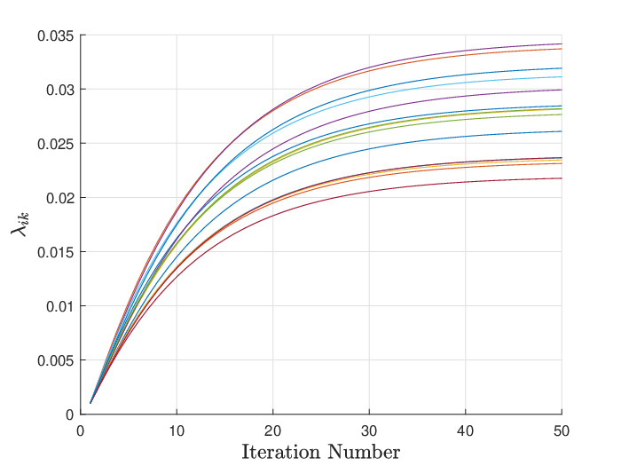
We first study the convergence behavior of the iterative algorithm proposed in Section IV-A to compute $\boldsymbol{\lambda}$ for the QoS problem ${\cal P}_{o}$ . Fig. 1 (left) shows the trajectory of $\lambda_{ik}$ over the number of iterations for each user with a normalized channel, for $N=50$ . To verify the asymptotic behavior of $\lambda_{ik}\beta_{ik}$ in Proposition 3, we consider users randomly located in the cell and generate their pathloss channels accordingly. Fig. 1 (right) shows the CDF of $\lambda_{ik}\beta_{ik}$ , with $\lambda_{ik}$ being computed by the iterative algorithm, for $N=50$ to 500. It is evident that as $N$ becomes large, all $\lambda_{ik}\beta_{ik}$ ’s converge to the same value, and the CDF converges to a step function.

Refer to caption — Fig. 1: Left: Convergence behavior of the iterative algorithm for $\{\lambda_{ik}\}$ ( $N=50$ , $G=3$ , $K=5$ ). Each curve represents $\lambda_{ik}$ of a user over iterations. Right: The CDF of $\lambda_{ik}\beta_{ik}$ for randomly generated user locations.

VI-2 Performance comparison for the QoS problem

We present the performance of using the optimal beamforming structure ${\bf w}_{i}^{o}$ in (18) and our proposed algorithms for the QoS problem ${\cal P}_{o}$ . Both SDR and SCA methods in Section IV-C are considered for computing weight vector ${\bf a}_{i}$ , and we name them OptBFwSDR and OptBFwSCA, respectively. Normalized channels are used. We also consider the following for comparison: 1) Lower bound for ${\cal P}_{o}$ : obtained by solving the relaxed problem of ${\cal P}_{o}$ via SDR, it serves as a benchmark for all algorithms; 2) AsymBFwSCA: the same as OptBFwSCA, except that ${\bf R}(\boldsymbol{\lambda})$ is approximated by (38); 3) Direct SDR: directly solve ${\cal P}_{o}$ for ${\bf w}$ via SDR with Gaussian randomization; 4) Direct SCA: directly solve ${\cal P}_{o}$ for ${\bf w}$ via the SCA method, taking the solution from the direct SDR as the initial point; 5) BDZF[18]: a low-complexity algorithm proposed recently for large-scale antenna arrays, using a two-layered approach combining block-diagonal ZF beamforming and SCA.⁹⁹ 9 Due to ZF beamforming, BDZF requires $N>K_{\text{tot}}-\min_{i\in{\cal G}}K_{i}$ . The computational complexity of SDR or SCA-based algorithm is analyzed in Sections IV-C1 and IV-C2, respectively. The complexity of BDZF is ${\cal O}(GN^{3})$ in each SCA iteration for $N\gg K$ .

TABLE I: Average Computation Time over

N

(sec.) (

G=3,K=5

, QoS).

$N$	50	100	200	300	400	500
OptBFwSDR	0.49	0.45	0.49	0.52	0.56	0.62
OptBFwSCA	1.61	1.37	1.51	1.40	1.41	1.42
BDZF[18]	11.5	34.1	182	495	605	N/A
Direct SDR	8.7	52.9	427	1509	4507	N/A
Direct SCA	7.41	44.2	353	1192	N/A	N/A

TABLE II: Average Computation Time over

K

(sec.) (

N=100,G=3

, QoS).

$K$	3	5	7	10	15
OptBFwSDR	0.44	0.48	0.68	1.03	1.89
OptBFwSCA	0.81	1.50	3.28	6.46	13.07
BDZF[18]	21.9	29.2	38.0	46.9	51.2
Direct SDR	33.5	50.6	69.4	98.4	136

TABLE III: Average Computation Time over

G

(sec.) (

N=100,K=5

$G$	2	3	4	5
OptBFwSDR	0.39	0.48	0.63	0.80
OptBFwSCA	0.86	1.50	2.77	4.52
BDZF[18]	16.5	27.0	40.2	49.2
Direct SDR	22.6	50.6	86.4	132.6

Denote the transmit power objective of ${\cal P}_{o}$ by $P_{t}\triangleq\sum_{i=1}^{G}\|{\bf w}_{i}\|^{2}$ . Fig. 2 shows the average normalized transmit power $P_{t}/\sigma^{2}$ vs. the number of antennas $N$ . Both OptBFwSCA and OptBFwSDR have consistent performance over a wide range of $N$ values. The performance of OptBFwSCA nearly attains the lower bound, while that of OptBFwSDR has a small gap of $\sim 0.3$ dB. Their performance is near-identical to their respective direct methods (direct SCA or direct SDR). The computational saving by using the optimal beamforming structure in OptBFwSCA and OptBFwSDR is evident in Table I, where the average computation time for different $N$ is shown (via MATLAB and CVX). Both OptBFwSCA and OptBFwSDR require very low computation time, which is kept roughly constant for all $N$ values. This is in contrast to the other alternative methods, whose computation times increase fast with $N$ and become impractical for large $N$ . OptBFwSCA performs better than OptBFwSDR by using SCA, at the cost of slightly higher computational complexity. Furthermore, we observe that AsymBFwSCA performs nearly identical to OptBFwSCA, indicating the effectiveness by using the closed-form asymptotic expression in (38) for ${\bf R}(\boldsymbol{\lambda})$ .

Fig. 3 presents the average normalized transmit power $P_{t}/\sigma^{2}$ vs. $K$ users per group for different $N$ values, when $G=3$ . OptBFwSCA performs very well and nearly attains the lower bound at all $K$ and $N$ values. For both OptBFwSDR and the direct SDR, the performance deteriorates over $K$ , which is known for the SDR-based methods as the number of constraints ( $K$ ) becomes large. The average computation time for the plots in Fig. 3 is shown in Table II. The increase of computation time over $K$ by OptBFwSDR is insignificant, while that of OptBFwSCA is more noticeable. Nevertheless, the computation time under both methods is still kept very low and is significantly lower than other methods. Also, to verify the performance of AsymBFwSCA, we plot it over $K$ for $N=300$ . Again, it shows a near-identical performance as OptBFwSCA. Fig. 4 shows the average normalized transmit power $P_{t}/\sigma^{2}$ vs. $G$ groups when $K=5$ , for different $N$ values. The corresponding average computation time is shown in Table III. The relative performance among different methods is similar to that in Fig. 3 for $K=5$ and $G=3$ and maintains the same as $G$ increases: both OptBFwSDR and OptBFwSCA provide near-optimal performance with very low computation time that only slightly increases over $G$ .

VI-3 Performance comparison for the MMF problem

We now present the performance using the optimal solution structure in (44) for the MMF problem ${\cal S}_{o}$ . The MMF beamformer is obtained via iteratively solving the QoS problem discussed in Section V, and the weight $\tilde{{\bf a}}_{i}$ is computed via the SDR (SCA) method, which we refer to as QoS2MMF-SDR (QoS2MMF-SCA). The pathloss channels are used. For comparison, we also consider the followings: 1) Upper bound of ${\cal S}_{o}$ : obtained by solving the relaxed version of ${\cal S}_{1}$ via SDR; 2) Direct SDR: direct solve the relaxed version of ${\cal S}_{1}$ via SDR with Gaussian randomization;¹⁰¹⁰ 10 In both 1) and 2), a bi-section search over $t$ is required along with SDR to obtain a solution. 3) AsymMMF-SCA: approximate $\widetilde{{\bf R}}(\boldsymbol{\lambda}_{\text{\tiny QoS}})$ by (48) and compute weight vector $\tilde{{\bf a}}_{i}$ by the SCA method as described below (48); 4) CF-AsymMMF: the closed-form asymptotic beamformer given in (49).

TABLE IV: Average Computation Time over

N

(sec.) (

G=3,K=5

, MMF).

$N$	50	100	200	300	400	500
QoS2MMF-SDR	6.77	7.26	7.54	7.75	8.88	9.96
QoS2MMF-SCA	27.6	29.9	27.6	30.0	33.7	37.6
AsymMMF-SCA	17.4	17.8	18.4	17.2	17.8	17.1
Direct SDR	162	1158	9924	N/A	N/A	N/A

TABLE V: Average Computation Time over

K

(sec.) (

N=100,G=3

, MMF).

$K$	3	5	7	10
QoS2MMF-SDR	5.65	7.16	8.81	14.6
QoS2MMF-SCA	18.3	22.7	27.7	39.3
AsymMMF-SCA	7.21	10.7	16.2	30.3
Direct SDR	457	766	1018	1359

Fig. 6 shows the average minimum SINR vs. $N$ , and Table V shows the corresponding computation time. The observations are similar to that in the QoS problem, where both QoS2MMF-SCA and QoS2MMF-SDR provide near-optimal performance, with a substantially lower computation time that only increases slightly over $N$ . Furthermore, AsymMMF-SCA performs as good as QoS2MM-SCA, with a further lower computation time roughly constant over $N$ . This verifies the asymptotic expression of $\widetilde{{\bf R}}(\boldsymbol{\lambda}_{\text{\tiny QoS}})$ in (48) and the effectiveness of this efficient method for the MMF problem. In contrast, CF-AsymMMF converges to the upper bound slower over $N$ , with a more noticeable performance gap observed due to the simple closed-form asymptotic weights used. Nonetheless, it offers much better performance with a significantly improved convergence rate than the existing asymptotic beamformers [45, 32], with less than 1dB gap at $N=500$ (as compared to $N$ being a few thousands in those works).

Finally, Fig. 6 shows the average minimum SINR vs. $K$ , with the computation time shown in Table V. The observations are similar to that in the QoS problem, where both QoS2MMF-SCA and AsymMMF-SCA show near-optimal performance at different $K$ values, and the computation time of the proposed methods is substantially lower than the direct SDR method.

VII Conclusion and Discussion

In this work, we obtained the optimal beamforming structure for the multi-group multicast beamforming, which has been unknown in the literature. Combining both the SCA numerical method and Lagrange duality, we derived the optimal multicast beamforming structure for both the QoS and MMF problems. This structure sheds light on the optimal multicast beamforming: 1) There is an uplink-downlink duality interpretation for the multicast beamforming problem, similar to the classical downlink multi-user unicast beamforming problem. 2) The optimal multicast beamformer is a weighted MMSE filter based on a group-channel direction, as a generalized version of the optimal downlink unicast beamformer. 3) There is an inherent low-dimensional structure in the optimal beamforming solution independent of $N$ , which brings opportunities for efficient numerical algorithms to compute the beamformer that is especially beneficial for systems with large antenna arrays. Using the optimal beamforming structure, we proposed efficient algorithms to compute the parameters in the optimal multicast beamformer. Characterizing the asymptotic behavior of the beamformers as $N$ grows large, we provided simple approximate multicast beamformers for large $N$ , including a closed-form asymptotic beamformer. They provide practical multicast beamforming solutions with near-optimal performance at very low computational complexity for massive MIMO systems.

The optimal multicast beamforming structure can be extended to multi-cell coordinated multicast beamforming scenarios, where the model difference is the per BS transmit power, instead of total power. For example, the MMF problem ${\cal S}_{o}$ has an inherent power allocation problem to $G$ groups, while for the multi-cell problem, the transmit power at each BS (to each group) is fixed. However, this difference is not expected to fundamentally change the optimal multicast beamforming structure, and the results obtained in this work can be extended to the multi-cell problem after some care of technical details.

Appendix A Proof of Corollary 2

Proof:

Since ${\cal P}_{\text{\tiny SCA}}({\bf z})$ is convex, its minimum objective can be obtained by its dual ${\cal D}_{\text{\tiny SCA}}({\bf z})$ . Rewrite $\boldsymbol{\nu}_{i}$ defined above (8) in a compact matrix form as $\boldsymbol{\nu}_{i}={\bf H}_{i}{\bf D}_{\boldsymbol{\lambda}_{i}}{\bf H}_{i}^{H}{\bf z}_{i}$ , where ${\bf D}_{\boldsymbol{\lambda}_{i}}\triangleq\diag(\boldsymbol{\lambda}_{i})$ . Then, the optimal ${\bf w}_{i}^{\star}({\bf z})$ in (11) can be rewritten as

\displaystyle{\bf w}_{i}^{\star}({\bf z})

\displaystyle={\bf R}_{i^{-}}^{-1}(\boldsymbol{\lambda}){\bf H}_{i}{\bf D}_{\boldsymbol{\lambda}_{i}}{\bf H}_{i}^{H}{\bf z}_{i}.

(50)

Substituting the above expression into (III-B), we have the dual function $g({\bf z},\boldsymbol{\lambda})$ in (6) as

$\displaystyle g({\bf z},\boldsymbol{\lambda})=$	$\displaystyle\sum_{i=1}^{G}\sum_{k=1}^{K_{i}}\lambda_{ik}(\sigma^{2}\gamma_{ik}+\|{\bf z}_{i}^{H}{\bf h}_{ik}\|^{2})$
	$\displaystyle+\sum_{i=1}^{G}{\bf z}_{i}^{H}{\bf H}_{i}{\bf D}_{\boldsymbol{\lambda}_{i}}{\bf H}_{i}^{H}{\bf R}_{i^{-}}^{-1}(\boldsymbol{\lambda}){\bf H}_{i}{\bf D}_{\boldsymbol{\lambda}_{i}}{\bf H}_{i}^{H}{\bf z}_{i}$
	$\displaystyle-2\sum_{i=1}^{G}\operatorname{\mathfrak{Re}}\{{\bf z}_{i}^{H}{\bf H}_{i}^{H}{\bf D}_{\boldsymbol{\lambda}_{i}}{\bf H}_{i}{\bf R}_{i^{-}}^{-1}(\boldsymbol{\lambda}){\bf H}_{i}{\bf D}_{\boldsymbol{\lambda}_{i}}{\bf H}_{i}^{H}{\bf z}_{i}\}$
$\displaystyle=$	$\displaystyle\sigma^{2}\sum_{i=1}^{G}\boldsymbol{\lambda}_{i}^{T}\boldsymbol{\gamma}_{i}+\sum_{i=1}^{G}{\bf z}_{i}^{H}{\bf H}_{i}{\bf D}_{\boldsymbol{\lambda}_{i}}{\bf H}_{i}^{H}{\bf z}_{i}$
	$\displaystyle-\sum_{i=1}^{G}{\bf z}_{i}^{H}{\bf H}_{i}{\bf D}_{\boldsymbol{\lambda}_{i}}{\bf H}_{i}^{H}{\bf R}_{i^{-}}^{-1}(\boldsymbol{\lambda}){\bf H}_{i}{\bf D}_{\boldsymbol{\lambda}_{i}}{\bf H}_{i}^{H}{\bf z}_{i}$
$\displaystyle=$	$\displaystyle\sum_{i=1}^{G}{\bf z}_{i}^{H}{\bf H}_{i}{\bf D}_{\boldsymbol{\lambda}_{i}}{\bf H}_{i}^{H}({\bf I}-{\bf R}_{i^{-}}^{-1}(\boldsymbol{\lambda}){\bf H}_{i}{\bf D}_{\boldsymbol{\lambda}_{i}}{\bf H}_{i}^{H}){\bf z}_{i}$
	$\displaystyle+\sigma^{2}\sum_{i=1}^{G}\boldsymbol{\lambda}_{i}^{T}\boldsymbol{\gamma}_{i}.$	(51)

From the optimal ${\bf w}_{i}^{o}$ expression in (22), based on the definition of $\alpha_{ik}^{o}$ , we have $\boldsymbol{\alpha}_{i}^{o}={\bf D}_{\boldsymbol{\lambda}_{i}^{o}}{\bf H}_{i}^{H}{\bf w}_{i}^{o}$ . Substituting this expression into (22), we have

\displaystyle{\bf w}_{i}^{o}

\displaystyle={\bf R}_{i^{-}}^{-1}(\boldsymbol{\lambda}^{o}){\bf H}_{i}{\bf D}_{\boldsymbol{\lambda}_{i}^{o}}{\bf H}_{i}^{H}{\bf w}_{i}^{o},\ i\in{\cal G},

or equivalently,

\displaystyle\left({\bf I}-{\bf R}_{i^{-}}^{-1}(\boldsymbol{\lambda}^{o}){\bf H}_{i}{\bf D}_{\boldsymbol{\lambda}_{i}^{o}}{\bf H}_{i}^{H}\right){\bf w}_{i}^{o}={\bf 0}.

(52)

As explained in the proof of Theorem 1, by the iterative procedure of the SCA method, if ${\bf z}_{i}$ converges to the optimum ${\bf z}_{i}\to{\bf w}_{i}^{o}$ in (51), the optimal $\boldsymbol{\lambda}^{\star}({\bf z})$ for the dual problem ${\cal D}_{\text{\tiny SCA}}({\bf z})$ also converges $\boldsymbol{\lambda}^{\star}({\bf z})\to\boldsymbol{\lambda}^{o}$ . By (52), it follows that

\displaystyle\max_{\boldsymbol{\lambda}}g({\bf w}^{o},\boldsymbol{\lambda})

\displaystyle=\sigma^{2}\sum_{i=1}^{G}{\boldsymbol{\lambda}_{i}^{o}}^{T}\boldsymbol{\gamma}_{i}=\sigma^{2}{\boldsymbol{\lambda}^{o}}^{T}\boldsymbol{\gamma}.

As ${\bf z}\to{\bf w}^{o}$ , ${\cal D}_{\text{\tiny SCA}}({\bf z})\to{\cal D}_{\text{\tiny SCA}}({\bf w}^{o})$ , ${\cal P}_{\text{\tiny SCA}}({\bf z})\to{\cal P}_{o}$ , and we obtain the minimum objective value of ${\cal P}_{o}$ as the above. ∎

Appendix B Proof of Proposition 2

Proof:

We first present the following lemma regarding the average of random variables.

Lemma 1.

Suppose $\{x_{n}\}$ is a sequence of i.i.d. random variables with $E(|x_{n}|)<\infty$ , $E(x_{n})=0$ , and $\{c_{n}\}$ is a bounded sequence, where $c_{n}$ is real, for all $n$ . Then, $\frac{1}{N}\sum_{n=1}^{N}c_{n}x_{n}\to 0$ almost surely (a.s.) as $N\to\infty$ .

Proof:

The result deals with an independent but not identically distributed sequence of random variables. It can be viewed as a variation of Kolmogorov’s Strong Law of Large Numbers (SLLN). The proof of this lemma follows the similar steps in the proof of SLLN, and thus is omitted here. The proof of SLLN can be found in [46, Theorem 7.5.1]. ∎Using Lemma 1, we have the following result.

Lemma 2.

Consider any two independent channel vectors ${\bf h}_{ik}$ and ${\bf h}_{il}$ , $l\neq k$ , each containing i.i.d. zero-mean elements. Then

\displaystyle\lim_{N\to\infty}\frac{1}{N}{\bf h}_{ik}^{H}{\bf R}^{-1}(\boldsymbol{\lambda}){\bf h}_{il}=0\ \ \text{a.s.}

(53)

Proof:

From the expression of ${\bf R}(\boldsymbol{\lambda})$ in (17), define

\displaystyle{\bf R}(\boldsymbol{\lambda};{ik}^{-})

\displaystyle\triangleq{\bf R}(\boldsymbol{\lambda})-\lambda_{ik}\gamma_{ik}{\bf h}_{ik}{\bf h}_{ik}^{H}.

(54)

To simplify the notation, let $\rho_{ik}\triangleq\lambda_{ik}\gamma_{ik}$ . Using the formula $({\bf A}+{\bf u}{\bf u}^{H})^{-1}={\bf A}^{-1}-\frac{{\bf A}^{-1}{\bf u}{\bf u}^{H}{\bf A}^{-1}}{1+{\bf u}^{H}{\bf A}^{-1}{\bf u}}$ , where ${\bf A}$ is an $n\times n$ matrix and ${\bf u}$ is an $n\times 1$ vector, we have

		$\displaystyle\hskip-10.00002pt{\bf h}_{ik}^{H}{\bf R}^{-1}(\boldsymbol{\lambda}){\bf h}_{il}={\bf h}_{ik}^{H}\left({\bf R}(\boldsymbol{\lambda};{ik}^{-})+\rho_{ik}{\bf h}_{ik}{\bf h}_{ik}^{H}\right)^{-1}{\bf h}_{il}$
		$\displaystyle={\bf h}_{ik}^{H}{\bf R}^{-1}(\boldsymbol{\lambda};{ik}^{-}){\bf h}_{il}\Big(\!1\!-\!\frac{\rho_{ik}{\bf h}_{ik}^{H}{\bf R}^{-1}(\boldsymbol{\lambda};{ik}^{-}){\bf h}_{ik}}{1+\rho_{ik}{\bf h}_{ik}^{H}{\bf R}^{-1}(\boldsymbol{\lambda};{ik}^{-}){\bf h}_{ik}}\!\Big)$
		$\displaystyle=\frac{{\bf h}_{ik}^{H}{\bf R}^{-1}(\boldsymbol{\lambda};{ik}^{-}){\bf h}_{il}}{1+\rho_{ik}{\bf h}_{ik}^{H}{\bf R}^{-1}(\boldsymbol{\lambda};{ik}^{-}){\bf h}_{ik}},\quad\forall k,l,i.$		(55)

For $l\neq k$ , define ${\bf R}(\boldsymbol{\lambda};(ik,il)^{-})\triangleq{\bf R}(\boldsymbol{\lambda};{ik}^{-})-\rho_{il}{\bf h}_{il}{\bf h}_{il}^{H}$ . Using ${\bf R}(\boldsymbol{\lambda};(ik,il)^{-})$ , we apply the same procedure above to ${\bf h}_{ik}^{H}{\bf R}^{-1}(\boldsymbol{\lambda};{ik}^{-}){\bf h}_{il}$ in (55) again and obtain (56). Note that, by our construction, ${\bf R}(\boldsymbol{\lambda};(ik,il)^{-})$ at the right-hand side (RHS) of (56) is no longer a function of ${\bf h}_{ik}$ or ${\bf h}_{il}$ .

\displaystyle{\bf h}_{ik}^{H}{\bf R}^{-1}(\boldsymbol{\lambda}){\bf h}_{il}=

\displaystyle\frac{{\bf h}_{ik}^{H}{\bf R}^{-1}(\boldsymbol{\lambda};(ik,il)^{-}){\bf h}_{il}}{(1+\rho_{ik}{\bf h}_{ik}^{H}{\bf R}^{-1}(\boldsymbol{\lambda};{ik}^{-}){\bf h}_{ik})(1+\rho_{il}{\bf h}_{il}^{H}{\bf R}^{-1}(\boldsymbol{\lambda};(ik,il)^{-}){\bf h}_{il})},\quad l\neq k.

(56)

Let ${\bf R}^{-1}(\boldsymbol{\lambda};(ik,il)^{-})={\bf U}\boldsymbol{\Delta}{\bf U}^{H}$ , where $\boldsymbol{\Delta}$ is a diagonal matrix containing the eigenvalues $\{\delta_{n}\}$ of ${\bf R}^{-1}(\boldsymbol{\lambda};(ik,il)^{-})$ . We have

\displaystyle\hskip-6.00006pt{\bf h}_{ik}^{H}{\bf R}^{-1}(\boldsymbol{\lambda};(ik,il)^{-}){\bf h}_{il}

\displaystyle=\tilde{{\bf h}}_{ik}^{H}\boldsymbol{\Delta}\tilde{{\bf h}}_{il}=\!\sum_{n=1}^{N}\delta_{n}\tilde{h}_{ik,n}^{*}\tilde{h}_{il,n}

(57)

where $\tilde{{\bf h}}_{ik}=[\tilde{h}_{ik,1},\ldots,\tilde{h}_{ik,N}]^{T}\triangleq{\bf U}^{H}{\bf h}_{ik}$ , and $\tilde{{\bf h}}_{il}$ is similarly defined. For ${\bf h}_{ik}$ and ${\bf h}_{il}$ being independent and zero-mean, $\tilde{{\bf h}}_{ik}$ and $\tilde{{\bf h}}_{il}$ are also independent and zero-mean. Let $x_{n}=\tilde{h}_{ik,n}^{*}\tilde{h}_{il,n}$ . We have $E(x_{n})=E(\tilde{h}_{ik,n}^{*})E(\tilde{h}_{il,n})=0$ . Since $\lambda_{i,k}\geq 0$ , from the structure of ${\bf R}(\boldsymbol{\lambda};(ik,il)^{-})$ , it is easy to see that $0<\delta_{n}\leq 1$ , $\forall n$ . Thus, the sequence $\{\delta_{n},1\leq n\leq N\}$ is bounded (for any given $N$ ). By Lemma 1, we have $\frac{1}{N}\sum_{n=1}^{N}\delta_{n}\tilde{h}_{ik,n}^{*}\tilde{h}_{il,n}\to 0$ a.s., or equivalently,

\displaystyle\lim_{N\to\infty}\frac{1}{N}{\bf h}_{ik}^{H}{\bf R}^{-1}(\boldsymbol{\lambda};(ik,il)^{-}){\bf h}_{il}

\displaystyle=0\ \ \text{a.s.}

(58)

Applying this to (56), we have (53), for $l\neq k$ . ∎

By (55), we have

\displaystyle{\bf h}_{ik}^{H}{\bf R}^{-1}(\boldsymbol{\lambda}){\bf h}_{ik}

\displaystyle=\frac{{\bf h}_{ik}^{H}{\bf R}^{-1}(\boldsymbol{\lambda};{ik}^{-}){\bf h}_{ik}}{1+\rho_{ik}{\bf h}_{ik}^{H}{\bf R}^{-1}(\boldsymbol{\lambda};{ik}^{-}){\bf h}_{ik}}.

(59)

Similar to (57), by decomposing ${\bf R}^{-1}(\boldsymbol{\lambda};ik^{-})$ , we have

\displaystyle\frac{1}{N}{\bf h}_{ik}^{H}{\bf R}^{-1}(\boldsymbol{\lambda};ik^{-}){\bf h}_{ik}

\displaystyle=\frac{1}{N}\sum_{n=1}^{N}\delta_{n}^{\prime}|\tilde{h}_{ik,n}^{\prime}|^{2}

(60)

where ${\bf R}^{-1}(\boldsymbol{\lambda};ik^{-})={\bf U}^{\prime}\boldsymbol{\Delta}^{\prime}{\bf U}^{\prime H}$ with $\boldsymbol{\Delta}^{\prime}\triangleq\diag([\delta^{\prime}_{1},\ldots,\delta^{\prime}_{N}])$ , and $\tilde{{\bf h}}_{ik}^{\prime}\triangleq{\bf U}^{\prime H}{\bf h}_{ik}$ with $\tilde{h}^{\prime}_{ik,n}$ being the $n$ th element in $\tilde{{\bf h}}_{ik}^{\prime}$ . Since elements in ${\bf h}_{ik}$ are i.i.d., $\tilde{h}^{\prime}_{ik,n}$ ’s are i.i.d. Also similarly, we have $0<\delta^{\prime}_{n}\leq 1$ , $\forall n$ , for ${\bf R}^{-1}(\boldsymbol{\lambda};ik^{-})$ . Denote $E(|\tilde{h}_{ik,n}^{\prime}|^{2})\triangleq\sigma_{h,ik}^{2}$ and define $x_{n}\triangleq|\tilde{h}_{ik,n}^{\prime}|^{2}-\sigma_{h,ik}^{2}$ . It is easy to verify that $\{x_{n}\}$ and $\{\delta^{\prime}_{n}\}$ satisfy the conditions in Lemma 1, and thus we have, as $N\to\infty$ , $\frac{1}{N}\sum_{n=1}^{N}\delta_{n}^{\prime}(|\tilde{h}_{ik,n}^{\prime}|^{2}-\sigma_{h,ik}^{2})\to 0~\text{a.s.}$ , or equivalently,

\displaystyle\frac{1}{N}{\bf h}_{ik}^{H}{\bf R}^{-1}(\boldsymbol{\lambda};ik^{-}){\bf h}_{ik}-\frac{\sigma_{h,ik}^{2}}{N}\sum_{n=1}^{N}\delta_{n}^{\prime}\to 0\ \ \text{a.s.}

(61)

Applying this to (59), we have $\lim_{N\to\infty}\frac{1}{N}{\bf h}_{ik}^{H}{\bf R}^{-1}(\boldsymbol{\lambda}){\bf h}_{ik}=c~~\text{a.s.}$ , for some $c>0$ .¹¹¹¹ 11 It can be shown by contradiction; Otherwise, (34) would not hold.

For $\lambda_{ik}$ being the solution of (34), by Lemma 2 and the above result, we have

		$\displaystyle\lambda_{ik}(1+\gamma_{ik}){\bf h}_{ik}^{H}{\bf R}^{-1}(\boldsymbol{\lambda}){\bf h}_{il}$
		$\displaystyle=\frac{{\bf h}_{ik}^{H}{\bf R}^{-1}(\boldsymbol{\lambda}){\bf h}_{il}}{{\bf h}_{ik}^{H}{\bf R}^{-1}(\boldsymbol{\lambda}){\bf h}_{ik}}=\frac{{\bf h}_{ik}^{H}{\bf R}^{-1}(\boldsymbol{\lambda}){\bf h}_{il}/N}{{\bf h}_{ik}^{H}{\bf R}^{-1}(\boldsymbol{\lambda}){\bf h}_{ik}/N}\to 0\ \ \text{a.s.}$

as $N\to\infty$ , for $\forall k,l\in{\cal K}_{i}$ and $l\neq k$ . Thus, the second equation in (33) asymptotically holds, and (32) asymptotically holds. Since (32) is a sufficient condition for (31), it follows that (31) also asymptotically holds. In other words, the solution $\boldsymbol{\lambda}$ of (34) converges to the solution of (31) almost surely. ∎

Appendix C Proof of Proposition 3

Proof:

From (34) and (59), we have, for $\forall\ k\in{\cal K}_{i},i\in{\cal G}$ ,

\displaystyle\frac{\lambda_{ik}(1+\gamma_{ik}){\bf h}_{ik}^{H}{\bf R}^{-1}(\boldsymbol{\lambda};{ik}^{-})^{-1}{\bf h}_{ik}}{1+\rho_{ik}{\bf h}_{ik}^{H}{\bf R}^{-1}(\boldsymbol{\lambda};{ik}^{-})^{-1}{\bf h}_{ik}}=1.

(62)

Substituting $\rho_{ik}=\lambda_{ik}\gamma_{ik}$ back into (62), bringing the denominator to the RHS, and removing the common terms at both sides, we have

\displaystyle\lambda_{ik}=\frac{1}{{\bf h}_{ik}^{H}{\bf R}^{-1}(\boldsymbol{\lambda};{ik}^{-})^{-1}{\bf h}_{ik}}.

(63)

Following (60), we note that $\tilde{{\bf h}}^{\prime}_{ik}$ and ${\bf h}_{ik}$ have the same distribution. Thus, for ${\bf h}_{ik}=\sqrt{\beta_{ik}}{\bf g}_{ik}$ with ${\bf g}_{ik}\sim{\cal C}{\cal N}({\bf 0},{\bf I})$ , we have $E(|\tilde{h}_{ik,n}^{\prime}|^{2})=\beta_{ik}$ . By (61) and the fact that $\sum_{n=1}^{N}\delta^{\prime}_{n}={\rm tr}(\boldsymbol{\Delta}^{\prime})={\rm tr}({\bf R}^{-1}(\boldsymbol{\lambda};ik^{-}))$ , we have, as $N\to\infty$ ,

\displaystyle\hskip-5.0pt\frac{1}{N}{\bf h}_{ik}^{H}{\bf R}^{-1}(\boldsymbol{\lambda};ik^{-}){\bf h}_{ik}-\frac{\beta_{ik}}{N}{\rm tr}({\bf R}^{-1}(\boldsymbol{\lambda};ik^{-}))\to 0\ \text{a.s.}

(64)

From (63) and (64), it follows that, as $N\to\infty$ ,

\displaystyle\frac{\frac{1}{N}}{\frac{1}{N}{\bf h}_{ik}^{H}{\bf R}^{-1}(\boldsymbol{\lambda};{ik}^{-})^{-1}{\bf h}_{ik}}-\frac{\frac{1}{N}}{\frac{\beta_{ik}}{N}{\rm tr}({\bf R}^{-1}(\boldsymbol{\lambda};ik^{-}))}\to 0\ \ \text{a.s.}

Thus, we have, as $N\to\infty$ ,

\displaystyle\lambda_{ik}\beta_{ik}

\displaystyle-\frac{1}{{\rm tr}({\bf R}^{-1}(\boldsymbol{\lambda};ik^{-}))}\to 0\ \ \text{a.s.}

(65)

By Jensen’s inequality, $\frac{1}{\frac{1}{N}{\rm tr}({\bf R}^{-1}(\boldsymbol{\lambda};ik^{-}))}\leq\frac{1}{N}{\rm tr}({\bf R}(\boldsymbol{\lambda};ik^{-}))$ . For ${\bf h}_{ik}=\sqrt{\beta_{ik}}{\bf g}_{ik}$ , we have

	$\displaystyle\frac{\frac{1}{N}}{\frac{1}{N}{\rm tr}({\bf R}^{-1}(\boldsymbol{\lambda};ik^{-}))}$	$\displaystyle\leq\frac{1}{N^{2}}{\rm tr}({\bf R}(\boldsymbol{\lambda};ik^{-}))$
	$\displaystyle=\frac{1}{N}$	$\displaystyle\Big[1+\mathop{\sum\sum}_{jl\neq ik}\lambda_{jl}\beta_{jl}\gamma_{jl}\Big(\frac{1}{N}\sum_{n=1}^{N}\|g_{jl,n}\|^{2}\Big)\Big]$

Note by Jensen’s inequality that, the gap between two sides of the above inequality reduces when the difference between the diagonal elements of $\frac{1}{N}{\bf R}(\boldsymbol{\lambda};ik^{-})$ reduces¹²¹² 12 For convex function $f(x)$ , as the range of $x$ becomes smaller, $f(x)$ is closer to a linear function.. In this case, the above bound becomes tight, and inequality becomes equality. Examining the diagonal elements, $[\frac{1}{N}{\bf R}(\boldsymbol{\lambda};ik^{-})]_{nn}=\frac{1}{N}(1+\mathop{\sum\sum}_{jl\neq ik}\lambda_{jl}\beta_{jl}\gamma_{jl}|g_{jl,n}|^{2})$ , for all $n$ , we verify that they have diminishing variance among them as $N\to\infty$ . It follows that, for (65), as $N\to\infty$ ,

\displaystyle\lambda_{ik}\beta_{ik}-\frac{1}{N}(1+\mathop{\sum\sum}_{jl\neq ik}\lambda_{jl}\beta_{jl}\gamma_{jl})\to 0\ \ \text{a.s.}

Let $\bar{\lambda}_{ik}\triangleq\lambda_{ik}\beta_{ik}$ . Rewrite the above, we have, as $N\to\infty$ ,

\displaystyle\Big(1+\frac{\gamma_{ik}}{N}\Big)\bar{\lambda}_{ik}\to\frac{1+\sum_{j=1}^{G}\sum_{l=1}^{{\cal K}_{j}}\bar{\lambda}_{jl}\gamma_{jl}}{N}\ \ \text{a.s.}

(66)

for $\forall k\in{\cal K}_{i}$ , $i\in{\cal G}$ , where the RHS limit is the same for all $k\in{\cal K}_{i}$ , $i\in{\cal G}$ . It follows that for $k\in{\cal K}_{i},l\in{\cal K}_{j},i,j\in{\cal G}$ , $ik\neq jl$ , as $N\to\infty$ ,

\displaystyle\frac{\bar{\lambda}_{jl}}{\bar{\lambda}_{ik}}=\frac{1+\gamma_{ik}/N}{1+\gamma_{jl}/N}=1+{\cal O}\Big(\frac{1}{N}\Big).

Substituting $\bar{\lambda}_{jl}=\bar{\lambda}_{ik}\big(1+{\cal O}\big(\frac{1}{N}\big)\big)$ , for $jl\neq ik$ , into the RHS of (66), we have, as $N\to\infty$ ,

\displaystyle\bar{\lambda}_{ik}\!

\displaystyle=\frac{1}{\displaystyle N\!-\!\mathop{\sum\sum}_{jl\neq ik}\gamma_{jl}-{\cal O}\Big(\frac{1}{N}\Big)}\!=\frac{1}{\displaystyle N\!-\!\mathop{\sum\sum}_{jl\neq ik}\gamma_{jl}}+o\Big(\!\frac{1}{N^{2}}\!\Big)

which is (36). ∎

References

[1] M. Dong and Q. Wang, “Optimal multi-group multicast beamforming structure,” in Proc. IEEE Int. Workshop on Signal Process. advances in Wireless Commun.(SPAWC), Jul. 2019.
[2] N. Sidiropoulos, T. Davidson, and Z.-Q. Luo, “Transmit beamforming for physical-layer multicasting,” IEEE Trans. Signal Process., vol. 54, pp. 2239–2251, Jun. 2006.
[3] M. A. Maddah-Ali and U. Niesen, “Fundamental limits of caching,” IEEE Trans. Inf. Theory, vol. 60, no. 5, pp. 2856–2867, 2014.
[4] S. Wu, W.-K. Ma, and A.-C. So, “Physical-layer multicasting by stochastic transmit beamforming and Alamouti space-time coding,” IEEE Trans. Signal Process., vol. 61, pp. 4230–4245, Sept 2013.
[5] A. Abdelkader, A. Gershman, and N. Sidiropoulos, “Multiple-antenna multicasting using channel orthogonalization and local refinement,” IEEE Trans. Signal Process., vol. 58, pp. 3922–3927, Jul. 2010.
[6] E. Karipidis, N. Sidiropoulos, and Z.-Q. Luo, “Quality of service and max-min fair transmit beamforming to multiple cochannel multicast groups,” IEEE Trans. Signal Process., vol. 56, pp. 1268–1279, 2008.
[7] T.-H. Chang, Z.-Q. Luo, and C.-Y. Chi, “Approximation bounds for semidefinite relaxation of max-min-fair multicast transmit beamforming problem,” IEEE Trans. Signal Process., vol. 56, pp. 3932–3943, 2008.
[8] D. Christopoulos, S. Chatzinotas, and B. Ottersten, “Weighted fair multicast multigroup beamforming under per-antenna power constraints,” IEEE Trans. Signal Process., vol. 62, pp. 5132–5142, Oct. 2014.
[9] M. Jordan, X. Gong, and G. Ascheid, “Multicell multicast beamforming with delayed SNR feedback,” in Proc. IEEE Global Telecommn. Conf. (GLOBECOM), Nov. 2009.
[10] Z. Xiang, M. Tao, and X. Wang, “Coordinated multicast beamforming in multicell networks,” IEEE Trans. Wireless Commun., vol. 12, pp. 12–21, Jan. 2013.
[11] Z. Luo, W. Ma, A. M. So, Y. Ye, and S. Zhang, “Semidefinite relaxation of quadratic optimization problems,” IEEE Signal Process. Mag., vol. 27, no. 3, pp. 20–34, May 2010.
[12] Z.-Q. Luo, N. Sidiropoulos, P. Tseng, and S. Zhang, “Approximation bounds for quadratic optimization with homogeneous quadratic constraints,” SIAM J. Optim., vol. 18, pp. 1–28, 2007.
[13] F. Rusek, D. Persson, B. K. Lau, E. G. Larsson, T. L. Marzetta, O. Edfors, and F. Tufvesson, “Scaling up MIMO: Opportunities and challenges with very large arrays,” IEEE Signal Process. Mag., vol. 30, pp. 40–60, Jan. 2013.
[14] B. R. Marks and G. P. Wright, “A general inner approximation algorithm for nonconvex mathematical programs,” Oper. Res., vol. 26, pp. 681–683, 1978.
[15] L. Tran, M. F. Hanif, and M. Juntti, “A conic quadratic programming approach to physical layer multicasting for large-scale antenna arrays,” IEEE Signal Processing Lett., vol. 21, pp. 114–117, 2014.
[16] D. Christopoulos, S. Chatzinotas, and B. Ottersten, “Multicast multigroup beamforming for per-antenna power constrained large-scale arrays,” in Proc. IEEE Workshop on Signal Processing Advances in Wireless Commun.(SPAWC), Jun. 2015, pp. 271–275.
[17] G. Scutari, F. Facchinei, L. Lampariello, S. Sardellitti, and P. Song, “Parallel and distributed methods for constrained nonconvex optimization-part II: Applications in communications and machine learning,” IEEE Trans. Signal Process., vol. 65, no. 8, pp. 1945–1960, Apr. 2017.
[18] M. Sadeghi, L. Sanguinetti, R. Couillet, and C. Yuen, “Reducing the computational complexity of multicasting in large-scale antenna systems,” IEEE Trans. Wireless Commun., vol. 16, pp. 2963–2975, May 2017.
[19] E. Chen and M. Tao, “ADMM-based fast algorithm for multi-group multicast beamforming in large-scale wireless systems,” IEEE Trans. Commun., vol. 65, pp. 2685–2698, Jun. 2017.
[20] J. Yu and M. Dong, “Low-complexity weighted MRT multicast beamforming in massive MIMO cellular networks,” in Proc. IEEE Int. Conf. Acoust., Speech, and Signal Process. (ICASSP), Apr. 2018, pp. 3849–3853.
[21] ——, “Distributed low-complexity multi-cell coordinated multicast beamforming with large-scale antennas,” in Proc. IEEE Int. Workshop on Signal Process. advances in Wireless Commun.(SPAWC), Jun. 2018.
[22] X. Wen, K. Law, S. Alabed, and M. Pesavento, “Rank-two beamforming for single-group multicasting networks using OSTBC,” in IEEE Sensor Array and Multichannel Signal Process. Workshop, Jun. 2012, pp. 69–72.
[23] I. H. Kim, D. Love, and S. Park, “Optimal and successive approaches to signal design for multiple antenna physical layer multicasting,” IEEE Trans. Commun., vol. 59, pp. 2316–2327, Aug. 2011.
[24] N. Bornhorst, M. Pesavento, and A. Gershman, “Distributed beamforming for multi-group multicasting relay networks,” IEEE Trans. Signal Process., vol. 60, pp. 221–232, Jan. 2012.
[25] M. Dong and B. Liang, “Multicast relay beamforming through dual approach,” in Proc. IEEE Int. Workshops on Computational Advances in Multi-Channel Sensor Array Process. (CAMSAP), Dec. 2013.
[26] K. T. Phan, S. A. Vorobyov, N. D. Sidiropoulos, and C. Tellambura, “Spectrum sharing in wireless networks via QoS-aware secondary multicast beamforming,” IEEE Trans. Signal Process., vol. 57, pp. 2323–2335, Jun. 2009.
[27] M. Tao, E. Chen, H. Zhou, and W. Yu, “Content-centric sparse multicast beamforming for cache-enabled cloud RAN,” IEEE Trans. Wireless Commun., vol. 15, no. 9, pp. 6118–6131, Sep. 2016.
[28] S. Boyd and L. Vandenberghe, Convex Optimization. Cambridge University Press, 2004.
[29] Y. Huang and D. Palomar, “Rank-constrained separable semidefinite programming with applications to optimal beamforming,” IEEE Trans. Signal Process., vol. 58, pp. 664–678, 2010.
[30] Z. Xiang, M. Tao, and X. Wang, “Massive MIMO multicasting in noncooperative cellular networks,” IEEE J. Sel. Areas Commun., vol. 32, no. 6, pp. 1180–1193, Jun. 2014.
[31] O. Mehanna, K. Huang, B. Gopalakrishnan, A. Konar, and N. D. Sidiropoulos, “Feasible point pursuit and successive approximation of non-convex QCQPs,” IEEE Signal Process. Lett., vol. 22, pp. 804–808, Jul. 2015.
[32] M. Sadeghi and C. Yuen, “Multi-cell multi-group massive MIMO multicasting: An asymptotic analysis,” in Proc. IEEE Global Telecommn. Conf. (GLOBECOM), Dec. 2015.
[33] H. Joudeh and B. Clerckx, “Rate-splitting for max-min fair multigroup multicast beamforming in overloaded systems,” IEEE Trans. Wireless Commun., vol. 16, no. 11, pp. 7276–7289, Nov. 2017.
[34] H. Chen, D. Mi, B. Clerckx, Z. Chu, J. Shi, and P. Xiao, “Joint power and subcarrier allocation optimization for multigroup multicast systems with rate splitting,” IEEE Trans. Veh. Technol., vol. 69, no. 2, pp. 2306–2310, Feb. 2020.
[35] O. Tervo, L. Trant, S. Chatzinotas, B. Ottersten, and M. Juntti, “Multigroup multicast beamforming and antenna selection with rate-splitting in multicell systems,” in Proc. IEEE Workshop on Signal Processing Advances in Wireless Commun.(SPAWC), Jun. 2018.
[36] O. Tervo, L. Tran, H. Pennanen, S. Chatzinotas, B. Ottersten, and M. Juntti, “Energy-efficient multicell multigroup multicasting with joint beamforming and antenna selection,” IEEE Trans. Signal Process., vol. 66, no. 18, pp. 4904–4919, Sep. 2018.
[37] A. Z. Yalcin and M. Yuksel, “Precoder design for multi-group multicasting with a common message,” IEEE Trans. Commun., vol. 67, no. 10, pp. 7302–7315, Oct. 2019.
[38] S. Kay, Fundamentals of Statistical Signal Processing: Estimation Theory. Englewood Cliffs, NJ 07632: Prentice Hall, 1993.
[39] F. Rashid-Farrokhi, K. J. R. Liu, and L. Tassiulas, “Transmit beamforming and power control for cellular wireless systems,” IEEE J. Sel. Areas Commun., vol. 16, no. 8, pp. 1437–1450, Oct. 1998.
[40] E. Visotsky and U. Madhow, “Optimum beamforming using transmit antenna arrays,” in Proc. IEEE Vehicular Technology Conf. (VTC), vol. 1, May 1999, pp. 851–856.
[41] M. Schubert and H. Boche, “Solution of the multiuser downlink beamforming problem with individual SINR constraints,” IEEE Trans. Veh. Technol., vol. 53, no. 1, pp. 18–28, Jan. 2004.
[42] E. Björnson, M. Bengtsson, and B. Ottersten, “Optimal multiuser transmit beamforming: A difficult problem with a simple solution structure [Lecture Notes],” IEEE Signal Process. Mag., vol. 31, no. 4, pp. 142–148, Jul. 2014.
[43] M. Lobo, L. Vandenberghe, S. Boyd, and H. Lebret, “Applications of second-order cone programming,” Linear Algebra and its Applications, vol. 284, pp. 193–228, 1998.
[44] S. Boyd, N. Parikh, and E. Chu, “Distributed optimization and statistical learning via the alternating direction method of multipliers,” Foundations and Trends in Machine Learning, vol. 3, no. 1, pp. 1–122, 2011.
[45] H. Zhou and M. Tao, “Joint multicast beamforming and user grouping in massive MIMO systems,” in Proc. IEEE Int. Conf. Commun. (ICC), Jun. 2015, pp. 1770–1775.
[46] S. I. Resnick, A probability path. Springer Science & Business Media, 2013.

		$\displaystyle{\cal P}_{1\text{\tiny SCA}}(\!{\bf v}\!):\min_{\{{\bf a}_{i}\}}\sum_{i=1}^{G}\\|{\bf G}_{i}{\bf a}_{i}\\|^{2}$
		$\displaystyle\text{subject~to~}\sum_{j=1}^{G}\|{\bf a}_{j}^{H}{\bf f}_{jik}\|^{2}-2\left(\!\frac{1}{\gamma_{ik}}\!+1\!\right)\ \operatorname{\mathfrak{Re}}\{{\bf a}_{i}^{H}{\bf f}_{iik}{\bf f}_{iik}^{H}{\bf v}_{i}\}$
		$\displaystyle\quad\quad+\left(\!\frac{1}{\gamma_{ik}}\!+1\!\right)\|{\bf v}_{i}^{H}{\bf f}_{iik}\|^{2}\leq-\sigma^{2},\ k\in{\cal K}_{i},i\in{\cal G}.$		(40)

Multi-group Multicast Beamforming: Optimal Structure and Efficient Algorithms

Abstract

Index Terms:

I Introduction

I-A Related Work

I-B Organization and Notations

II System Model and Problem Formulation

III Optimal Multicast Beamforming Structure

III-A The SCA Method

III-B The Optimal Multicast Beamforming Solution

Proposition 1.

Proof:

Theorem 1.

Proof:

Corollary 1.

Corollary 2.

Proof:

Corollary 3.

III-C Discussions on the Optimal Solution Structure

III-C1 Uplink-downlink duality interpretation

III-C2 Weighted MMSE beamforming structure

III-C3 Multicast versus unicast

III-C4 Inherent low-dimensional structure

IV Numerical Algorithms and Analysis

IV-A Algorithm for Lagrange Multiplier 𝛌\boldsymbol{\lambda}

IV-B Asymptotic Analysis of 𝛌\boldsymbol{\lambda}

Proposition 2.

Proof:

Proposition 3.

Proof:

IV-B1 Asymptotic 𝐑⁡(𝝀){\bf R}(\boldsymbol{\lambda})

IV-B2 Slow diminishing rate of interference

IV-C Algorithms for Weight Vector {𝐚i}\{{\bf a}_{i}\}

IV-C1 The SDR method

IV-C2 The SCA method

V Multicast Beamforming for the MMF Problem

Theorem 2.

Proof:

V-A Asymptotic MMF Multicast Beamforming Solution

VI Simulation Results

VI-1 Convergence behavior of the algorithm for 𝝀\boldsymbol{\lambda}

VI-2 Performance comparison for the QoS problem

VI-3 Performance comparison for the MMF problem

VII Conclusion and Discussion

Appendix A Proof of Corollary 2

Proof:

Appendix B Proof of Proposition 2

Proof:

Lemma 1.

Proof:

Lemma 2.

Proof:

Appendix C Proof of Proposition 3

Proof:

References

IV-A Algorithm for Lagrange Multiplier $\boldsymbol{\lambda}$

IV-B Asymptotic Analysis of $\boldsymbol{\lambda}$

IV-B1 Asymptotic ${\bf R}(\boldsymbol{\lambda})$

IV-C Algorithms for Weight Vector $\{{\bf a}_{i}\}$

VI-1 Convergence behavior of the algorithm for $\boldsymbol{\lambda}$