Unified SU(4) theory for the and anomalies
Abstract
We propose a chiral Pati-Salam theory based on the gauge group . The left-handed quarks and leptons are unified into a fundamental representation of , while right-handed quarks and leptons have a separate treatment. The deviations measured in the rare semileptonic decays are explained by a scalar leptoquark which couples to right-handed fields and is contained in the -breaking scalar multiplet. The measured deviation of lepton flavor universality in the rare decays , is explained via the leptoquark gauge boson. The model predicts a new sub-GeV scale sterile neutrino which participates in the anomaly and can be searched for in upcoming neutrino experiments. The theory satisfies the current most sensitive experimental constraints and its allowable parameter regions will be probed as more precise measurements from the LHCb and Belle II experiments become available.
Keywords:
B physics, lepton flavor universality, leptoquark, unified model, Pati-SalamI Introduction
The standard model (SM) of particle physics with the inclusion of neutrino masses describes nature with unprecedented precision and has so far withstood all experimental tests. However, recently several hints for a violation of lepton flavor universality (LFU) in recent measurements of semileptonic meson decays Aaij et al. 2014a; Aaij et al. 2017; Aaij et al. 2013; Aaij et al. 2016; Wehle et al. 2017; Aaij et al. 2014b; Aaij et al. 2015; Aaij et al. 2019a have emerged. The theoretically cleanest probes are the LFU ratios
| (1) |
where is a light lepton , because hadronic uncertainties cancel out in the LFU ratios Hiller and Kruger 2004. Their current experimental measurements and SM predictions are summarized in Table 1. While the LFU ratios point to a smaller decay rate with final state muons compared to electrons in the neutral current process , the LFU ratios indicate an enhanced rate for the charged current process compared to light charged leptons in the final state. The significance of the anomalies in semileptonic meson decays is at the level of for both and ratios, while the significance for the combined measurement of the LFU ratios and exceeds .
| Observed | SM | range | |
|---|---|---|---|
| Aaij et al. 2019a | Bobeth et al. 2007 | ||
| Aaij et al. 2017 | Bordone et al. 2016 | ||
| Amhis et al. 2018 | Bailey et al. 2015 | Full | |
| Amhis et al. 2018 | Fajfer et al. 2012 | Full |
The experimental anomalies in and are supported by a similar deviation in the LFU ratio which analogously points to a larger branching fraction to tau leptons compared to muons, although still being consistent with the SM at the level due to large experimental uncertainties Aaij et al. 2018a. Also, there are deviations in the angular observable Descotes-Genon et al. 2013; Guadagnoli 2017 and more generally data from several measurements of Descotes-Genon et al. 2016 that suggest a suppression of the decays compared to the SM expectation, while being consistent with the experimentally observed value of the LFU ratios . However, as these other channels currently have fewer clean signals due to large hadronic uncertainties in absolute branching ratio measurements and due to the difficulty of estimating a signal for Guadagnoli 2017 along with other experimental uncertainties, we instead focus on the LFU ratios introduced in Eq. (1) in the following discussion.
The possibility that some or even all of these deviations might be a harbinger of new physics has been entertained in the literature. In particular, several models Assad et al. 2018; Di Luzio et al. 2017; Calibbi et al. 2018; Bordone et al. 2018a; Barbieri and Tesi 2018; Blanke and Crivellin 2018; Greljo and Stefanek 2018; Bordone et al. 2018b; Faber et al. 2018; Heeck and Teresi 2018; Balaji et al. 2019; Fornal et al. 2019 have been proposed. Most of these models simultaneously explain the physics anomalies via a massive vector leptoquark 11 1 is the vector leptoquark in the nomenclature of Ref. Buchmuller et al. 1987., which is predicted by the breaking of . In particular chiral models Buttazzo et al. 2017; Balaji et al. 2019; Fornal et al. 2019 are phenomenologically motivated, because they avoid constraints from lepton-flavor-violating pseudoscalar meson decays like , which place stringent constraints on the -breaking scale Hung et al. 1982; Valencia and Willenbrock 1994; Smirnov 2007; Kuznetsov et al. 2012; Carpentier and Davidson 2010; Smirnov 2018. The authors of Ref. Hati et al. 2019 find that minimal models with a single vector leptoquark and a unitary quark-lepton mixing matrix are generally disfavored due to strong constraints from charged lepton-flavor-violating processes.
We pursue a different approach and build on our previously suggested Pati-Salam inspired chiral gauge model Balaji et al. 2019, where the anomaly is explained via the vector leptoquark with purely left-handed couplings. The explanation of is predictive and depends on only two parameters, the mass of the vector leptoquark and a CKM-type mixing angle between left-handed down-type quarks and charged leptons. One interesting feature of the model is the simultaneous modification of both the decay to muons, , and electrons22 2 Modifications to electrons have been suggested in Ref. Hiller and Schmaltz 2015 and also realized in the simultaneous explanation of both anomalies using the leptoquark Popov et al. 2019., , in opposite directions by an equal amount. Here, we consider a simple extension of the model with a larger gauge group which further unifies the right-handed matter fields. This allows explanation of the anomalies with a new scalar leptoquark 33 3 corresponds to the conjugate of the leptoquark in the nomenclature of Ref. Buchmuller et al. 1987., which is part of the scalar breaking of the Pati-Salam gauge group to the SM gauge group. The leptoquark is well known as an explanation for Sakaki et al. 2013; Freytsis et al. 2015 and other hints of new physics (see e.g. Refs. Bauer and Neubert 2016; Popov and White 2017; Cai et al. 2017; Azatov et al. 2018; Bigaran et al. 2019). Here, the leptoquark features purely right-handed couplings and thus mediates with right-handed charged fermions, where is a new light sterile neutrino. The sterile neutrino can be searched for and provides a smoking-gun signature of the explanation of the observed measurement of .
The paper is structured as follows. In Sec. II we introduce the model and discuss the scalar potential and fermion masses. New contributions to the physics anomalies are discussed in Sec. III and relevant constraints in Sec. IV. In Sec. V we present our results before concluding in Sec. VI. The decomposition of the particle content in terms of SM multiplets is shown in the appendix.
II Model
We propose a model based on the gauge group and assign the particle content such that the leptoquark gauge boson couples to the quarks and leptons in a chiral fashion. This naturally avoids strong constraints from charged lepton-flavor-violating leptonic neutral meson decays such as and . The particle content of the model is listed in Table 2.
| Fermion | Generations | Scalar | ) | |
|---|---|---|---|---|
| 3 | ||||
| 3 | ||||
| 3 | ||||
| 1 |
Apart from the usual matter fields in the fundamental representation of , there are three generations of right-handed triplet fermions and a left-handed total singlet fermion . The scalar sector consists of a bidoublet and two fields in the fundamental representation of , and .
The symmetry is broken by the vacuum expectation value (VEV) of the scalar at a high scale, TeV, where the first (second) index refers to the fundamental representation of (). Electroweak symmetry is broken by the scalar with where and refer to the VEVs in the and ( components. The combination of the VEVs of and induces small VEVs for , and . The first index refers to the fundamental representation of , the second refers to the fundamental representation of and the last two in round brackets are two indices in the fundamental representation of which are symmetrized as indicated by the round brackets, . Thus the following symmetry-breaking pattern emerges
| (2) |
Here weak hypercharge and electric charge are related to the generators in by and , respectively. If we use the gauge symmetry to rotate the VEV of to the fourth component, then is the diagonal traceless generator with elements .
II.1 Yukawa sector
Given the particle content in Table 2 the full Yukawa Lagrangian is given by
| (3) | ||||
where flavor indices are suppressed, but indices for the gauge groups are explicitly shown.44 4 Lower indices refer to the fundamental representation and upper indices refer to the antifundamental representation. Fields with lower indices transform as . The Yukawa couplings are matrices in flavor space; rows (columns) are labeled by the first (second) fermion in the fermion bilinear. Indices in fundamental representation of are labeled by roman letters , indices in the fundamental representation of are labeled by greek letters and indices in the fundamental representation of are labeled by roman letters . In the above expression we used the charge-conjugate fields and with . From the Yukawa Lagrangian (3) we obtain the Lagrangian of the quark masses
| (4) |
with the quark mass matrices
| (5) |
The charged and neutral lepton mass matrices can be written in the basis
| (6) |
with the mass matrices
| (7) |
A viable mass spectrum for the charged leptons is obtained for . More precisely, we take the eigenvalues of to be less than GeV and the eigenvalues of to be larger than TeV. In this case the new charged fermions decouple and their masses are determined by , while the light charged lepton masses are determined by . The contribution from mixing with can be neglected because of the assumed relative sizes of , and . In the basis of a diagonal the SM charged lepton mass eigenstates are approximately given by the weak interaction eigenstates. We thus denote them by . Neutrino mass eigenstates are labeled by . Hence in this basis the leptonic mixing matrix is determined by the neutrino mass matrix up to subpercent-level corrections from mixing with the heavy charged leptons.
The neutrino oscillation data and the existence of a fourth light sterile neutrino with GeV requires and to be satisfied. For the remainder of this work we focus exclusively on the limit in order to recover the experimentally observed active neutrino mass spectrum and the leptonic mixing angles. In this limit, three pseudo-Dirac pairs obtain masses of order and decouple from four light neutrinos. A minimal phenomenologically viable texture for the neutrino mass matrix is given by
| (8) |
The large off-diagonal entries and are required for the anomalies. The entries of the Majorana mass matrices and have to be small GeV in order to kinematically allow from the relevant process.
II.2 Scalar potential
In this model, the masses of the charged leptons arise from the VEV of the scalar, while the masses of the quarks result from the VEVs of the bidoublet . In such a situation, consistent Higgs phenomenology requires a decoupling limit where the LHC Higgs-like scalar is identified with the lightest neutral scalar in the model. The decoupling limit works analogously to the one shown in Refs. Haber and Nir 1990; Balaji et al. 2019 and thus, we do not repeat the whole discussion, but instead focus only on the pertinent differences in the following.
In order to achieve the desired symmetry-breaking pattern, we first neglect the scalar and focus on the scalars and . In this case the possible invariants which enter the scalar potential are
| (9) | ||||||
where we have subtracted the VEVs from each invariant such that the invariants vanish in the vacuum. The VEV of can always be chosen to be real by using a suitable global rotation. The terms , and respect an accidental symmetry. is broken by and is broken by . The invariants , and are non-negative, while the others may become negative and thus terms involving these have to be sufficiently small to ensure vacuum stability. As the discussion of the physics anomalies is mostly independent to the exact form of the scalar potential, we only comment on how to obtain the correct vacuum structure. The scalar potential in terms of invariants is given by
| (10) |
The coefficients parametrize interactions between the and fields. Most of the scalar potential is invariant under a larger symmetry group with two separate symmetries for each of the two scalars and . It is only broken to the diagonal subgroup by the last term . The couplings in the scalar potential can be chosen real due to the invariants in Eq. (9) being Hermitian. We also restrict ourselves to real VEVs. This potential allows the VEV hierarchy to emerge, which leads to the correct quark mass spectrum with and as mentioned in the previous section. The scalar doublet in the bidoublet which does not obtain a VEV induces flavor changing neutral currents Mohapatra et al. 1983; Gilman and Reno 1984; Gilman and Reno 1983; Ecker et al. 1983 which poses a lower bound on its mass scale of TeV Bertolini et al. 2014.
There are many terms in the scalar potential which couple the scalar field to other scalar fields. However most of them are not relevant for the induced VEVs of . The most important term is linear in
| (11) |
where we have absorbed the phase of by rephasing and defined the electrically neutral scalar . In order to calculate the induced VEV of the scalar it is sufficient to consider terms quadratic in , because the induced VEV is much smaller compared to all other scales. Thus we obtain
| (12) |
where is the mass of . In the limit the observed Higgs boson is a linear combination of and
| (13) |
The mixing arises from the term in Eq. (11) and indirectly from terms quadratic in and , after obtains a VEV . Generally the mixing angle is given by and thus the Higgs features SM-like couplings, as discussed in Refs. Haber and Nir 1990; Balaji et al. 2019.
III New contributions to semileptonic decays
In Ref. Balaji et al. 2019, we showed that the experimentally observed values of and can be explained via the exchange of the massive leptoquark gauge boson in . There has been a recent measurement of by the LHCb experiment Aaij et al. 2019a (see Table 1) and the LHCb experiment also published a new stronger limit Aaij et al. 2019b on the branching ratio of the semileptonic charged lepton flavor violating decay : BR and BR at 90% C.L. Hence we briefly summarize the relevant definitions in Sec. III.1 and update the analysis with the latest measurements in Sec. IV.
The aforementioned vector leptoquark cannot explain the measurement of and due to its chiral couplings. This model also features several scalar leptoquarks which also contribute to : (i) The scalar contains two leptoquarks and , denoted by and in the nomenclature of Ref. Buchmuller et al. 1987. However these two leptoquarks have chiral couplings and either couple to charged leptons or neutrinos, but not both simultaneously. Although their electric charge components mix and thus in general contribute to , their contribution is suppressed due to the small mixing and thus cannot account for the observed deviation in . (ii) The scalar also contains a leptoquark . We discuss its contributions to in Sec. III.2.
III.1 Neutral current process:
We briefly outline the most important points from the study in Ref. Balaji et al. 2019 and refer the interested reader to the publication for further details. The relevant gauge interactions with the fermions are given by
| (14) |
where is the gauge coupling constant and is the mixing matrix between left-handed charged leptons and down-type quarks as shown in Ref. Balaji et al. 2019. As quantum chromodynamics is embedded in , the coupling is directly defined by the strong gauge coupling. Here we have defined to include the three charged SM leptons and the three heavy exotic charged lepton mass eigenstates, i.e. .
After integrating out the heavy mediator with mass there are new contributions to the Wilson coefficients of ,
| (15) |
In the above is the running strong coupling constant and denotes the fine-structure constant evaluated at the electroweak scale. are the elements of a CKM-type quark-lepton mixing matrix. The Wilson coefficients are defined by the effective Lagrangian
| (16) |
where denotes operators with a strange and bottom quark and two charged leptons
| (17) |
In order to explain the anomalies and to avoid stringent constraints from the lepton-flavor-violating decays among others, a particular off-diagonal structure of the CKM-type quark-lepton mixing matrix is suggested. Considering only the first three columns of the general matrix, i.e. the part relevant to quark-SM lepton interactions, we adopt the limiting case 55 5 In general is a matrix which satisfies the unitarity condition , where is the unit matrix.
| (18) |
III.2 Charged current process:
The leptoquark couples to both charged leptons and neutrinos
| (19) |
Starting from this interaction Lagrangian we derive the Wilson coefficients. The neutrino mass eigenstate mixes with the flavor eigenstates and where denotes the matrix diagonalizing the neutral fermion mass matrix . The masses of the neutrino mass eigenstates are denoted , , where denotes the masses of the three active neutrinos, is the mass of the fourth mass eigenstate and labels the masses of the mostly heavy sterile neutrinos. We work in the basis where the right-handed charged leptons and the right-handed up-type quarks are given by their mass eigenstates. Then the relevant part of the interaction Lagrangian for reads
| (20) |
with , where relates the weak interaction eigenstates with the mass eigenstate . In the following we use and drop the primes from the mass eigenstates. Integrating out scalar results in
| (21) |
among other operators. The effective vector and axial-vector operators for a lepton and right-handed neutrino are defined according to Ref. Bardhan et al. 2017 as
| (22) |
and enter the effective Lagrangian
| (23) |
We may then simply compute the relevant Wilson coefficients required to compute which are given by
| (24) |
where we expressed in terms of the entries of the minimal Yukawa matrix structure defined in Eq. (8) and the matrix elements of .
Considering the aforementioned limit where , we may compute the mixing angles and for the fourth neutrino state
| (25) |
to leading order. So we note that with the selected Yukawa structure, the neutrino that participates in the anomalies is dominantly a mixture of the singlet and the second state in . Substituting the above mixing angles into (24) results in
| (26) |
As the decay rates are summed over all polarizations and spins, the expressions for the LFU ratios should be invariant after replacing all Wilson coefficients for left-handed currents by right-handed ones and vice versa Asadi et al. 2018. Hence, we may use the literature result for left-handed neutrinos Bardhan et al. 2017 and map them directly to right-handed neutrinos since there is no interference between left- and right-handed operators. The resulting (C.L.) bounds on from Table 1 can be directly converted to constraints on the right-handed neutrino current Wilson coefficient
| (27) |
IV Constraints
Several measurements already place constraints on the favored parameter region. In particular boson decays to charged leptons, semihadronic B-meson decays, and collider constraints for the leptoquark, cosmological, astrophysical and direct search constraints on the sterile neutrino .
IV.1 decay constraints
The new leptoquark modifies the decay width to muons at one-loop level due to the presence of a large Yukawa coupling . Contributions to other leptonic decays of the boson are generally small in this model. As the leptoquark only couples to right-handed charged leptons, its contribution can be parametrized by
| (28) |
following Ref. Arnan et al. 2019, where is the gauge coupling and the weak mixing angle. For the contribution of the leptoquark can simply be written as
| (29) |
to leading order, where . The current best experimental bound from precision electroweak physics comes from the LEP experiments Schael et al. 2006. We demand that the -boson coupling to muons is not changed by more than the experimental uncertainty at [90% C.L.], i.e. , and thus we obtain the constraint
| (30) |
IV.2
Another constraint comes from which is modified by the leptoquark . It is described by effective operators of the form Buras et al. 2015
| (31) |
Integrating out as before we obtain
| (32) |
As we find that the new physics contribution is very small compared to the SM contribution and thus does not provide any competitive constraint. Similarly, new contributions from the exchange of to and decay rates are very suppressed due to the assumed Yukawa coupling structure.
IV.3 Collider constraints
There currently does not exist a plethora of dedicated searches at colliders for the leptoquark since the chosen Yukawa texture by construction couples only second-generation quarks with third-generation leptons and vice versa. The most common LHC searches are for single generation leptoquarks Sirunyan et al. 2019a; Sirunyan et al. 2018; Sirunyan et al. 2018; Khachatryan et al. 2017; Khachatryan et al. 2014; Chatrchyan et al. 2012; Chatrchyan et al. 2013. The searches are commonly separated into single leptoquark and pair production. The latter is generally independent of the absolute magnitude of the leptoquark Yukawa coupling, because the leptoquarks are produced via strong interactions in a hadron collider, unless the Yukawa couplings are large and substantially contribute to the leptoquark production, while single leptoquark production depends on the Yukawa coupling.
The model parameter space can be most economically constrained by searches with or final states. The particle can also decay into due to the coupling being nonzero, but searches for final states with missing transverse energy are typically less sensitive. For the chosen mass range of the scalar leptoquark imposing the constraints from searches with third-generation scalar leptoquarks decaying into a tau lepton and a quark such as the analysis in Ref. Sirunyan et al. 2018 does not pose any additional constraint on the parameter space over the decay constraint, although the sensitivity on the quark is markedly improved due to tagging of the final state jets. However, a mixed 1-3 generation leptoquark search with final states analogous to the third-generation search in Ref. Khachatryan et al. 2015 could strengthen the limits on the coupling significantly in the future. Of course more complicated Yukawa textures for and (particularly the diagonal entries), can be chosen and constrained with the aforementioned single generations searches, however we do not consider these more complicated parametrizations in this work for the sake of brevity.
Finally there are constraints from the single -lepton + MET searches. The authors of Ref. Greljo et al. 2019 reinterpreted the searches for a heavy charged gauge boson from sequential SM (SSM) resonance searches of the ATLAS Aaboud et al. 2018 and CMS Sirunyan et al. 2019b experiments as constraints on models explaining . In particular, the leptoquark with purely right-handed couplings has been studied and the study finds that leptoquark masses above 2 TeV are excluded at more than . At face value this constrains the leptoquark to be lighter than 2 TeV. As the study was based on an older best fit to the anomalies further away from the SM, the current constraint for heavy charged gauge bosons from SSM resonance searches is relaxed and heavier masses are allowed. However, the precise value of the current constraint requires a new study. In the following results discussion, we thus consider leptoquark masses up to 3 TeV and caution the reader that the SSM resonance search poses a constraint on the heaviest allowable leptoquark masses according to the study shown in Ref. Greljo et al. 2019.
IV.4 Constraints on the sterile neutrino
The sterile neutrino as defined would be produced in the early Universe. The dominant decay modes are with for masses GeV. These decays are mediated by the boson and thus the decay rate depends quadratically on the mixing matrix element . In the limit of vanishing final state lepton masses, the decay rate of is given by Lee and Shrock 1977; Pal and Wolfenstein 1982; Barger et al. 1995
| (33) |
For the lifetime is given
| (34) |
Big bang nucleosynthesis (BBN) poses a constraint on the lifetime of , since the abundances of the light elements agree well with the standard cosmological model. Thus in order to avoid any changes to the standard BBN, the sterile neutrino has to decay and its decay products thermalize, before BBN. If the lifetime of is shorter than , this condition can be satisfied as it has been shown in Refs. Dolgov et al. 2000a; Dolgov et al. 2000b. This translates into a bound
| (35) |
Similarly, sterile neutrinos can be produced in supernovae. The arguments of Ref. Dolgov et al. 2000a imply that the duration of the SN 1987A neutrino burst excludes mixing angles for sterile neutrinos MeV.
Finally, sterile neutrinos can be searched for at terrestrial experiments. In particular the fixed-target experiments NOMAD Astier et al. 2001 and CHARM Orloff et al. 2002 placed limits on the mixing angle of sterile neutrinos with neutrinos, which further constrains the allowed parameter space, as discussed in Sec. V.
Together this puts a lower bound on the sterile neutrino mass of MeV.
V Results
As the explanations for the and anomalies are mostly independent, we first discuss the explanation of , which sets the scale of the symmetry breaking. As a second step, we present the favored region for the anomalies , before finally discussing its predictions for the sterile neutrino in the process .
V.1
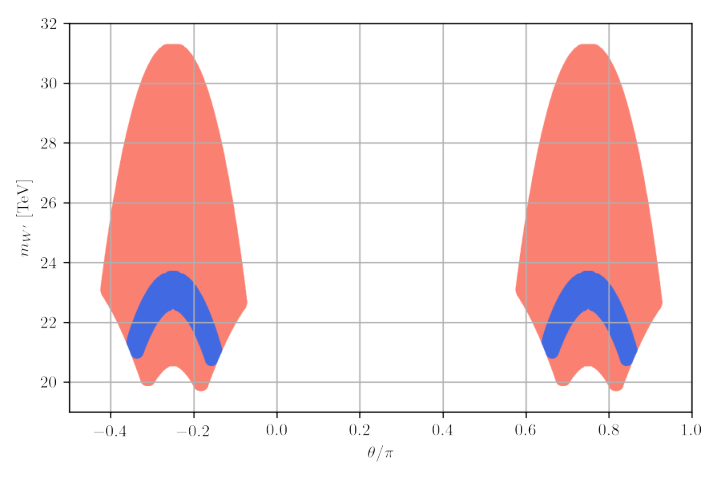
We follow our previous analysis Balaji et al. 2019 and identify the favored region of parameter space for the model using the flavio package Straub et al. 2018 and tree-level analytical estimations where appropriate. The (90% C.L.) favored parameter region is defined by the values of the vector leptoquark mass and the quark-SM lepton mixing angle [see Eq. (18) for its definition] which satisfy (), () and also satisfy the current 90% C.L. experimental limits and Tanabashi et al. 2018. Other processes currently do not constrain the parameter region as we discussed in Ref. Balaji et al. 2019.
Figure 1 shows the favored region of parameter space in the leptoquark mass versus the mixing angle plane. Compared to Ref. Balaji et al. 2019 the mass of is larger, because the experimentally observed value of has since moved closer to the SM prediction with smaller error bars and therefore the region is smaller. The favored range of is approximately between or and between TeV. The identical nature of the two adjacent regions can be understood from the invariance of the relevant branching ratios under the transformation . The constraints from lead to the wedge-shape form at the bottom of each favored region.


Figure 2 shows the predicted range for the branching ratios of the lepton-flavor-violating rare decays and processes. The two processes probe different ranges of values and are thus complementary: While is sensitive to , is sensitive to . LHCb is expected to further improve its sensitivity and to probe the two branching ratios of at the level of Aaij et al. 2018b.
In addition to further improvements to this leptoquark contributes to lepton-flavor-violating rare tau lepton decays such as , and the leptonic decays , as shown in Ref. Balaji et al. 2019. However, the additional contributions are below the current experimental sensitivity and thus we do not show these predictions for the sake of brevity and refer the interested reader to Ref. Balaji et al. 2019 for further details.
V.2
Using Eq. (26) along with the and C.L. constraints on the Wilson coefficient we may derive the allowable parameter region for the model which satisfies the anomalies. We restrict ourselves to placing bounds on the and C.L. region. Choosing the minimal Yukawa texture described in Sec. II.1 for and constrains the parameter region in , , and space.
We limit for our parameter scans to ensure that the lightest flavor exotic charged lepton mass is larger than TeV for scales larger than TeV, and this coupling does not affect the neutrino states and that participate in the anomaly and is therefore not important in constraining the model’s allowable region. The Yukawa couplings of interest must also satisfy perturbativity requirements such that , while in order to obtain Wilson coefficient with the correct sign. The VEV TeV was chosen for our parameter scans as this is a favored central value for the TeV gauge boson mass scale which explains the anomalies. This fixes the lightest exotic vectorlike lepton mass to TeV which easily evades the LEP constraints for heavy charged leptons Tanabashi et al. 2018.
We also set as this acts as an upper bound on the fourth neutrino mass participating in . This value is chosen because it ensures that the sterile neutrino decays before BBN. The analytical approximation for the mixing angles and in Eq. (25) and subsequently Eq. (26) is respected as well as ensuring that the new neutrino mass is light enough that it does not introduce too much phase space suppression in the decay . Consequently in our parameter scan we find the fourth neutrino mass to be lighter than the , but heavier than 100 MeV after imposing all constraints, which ensures that it is still significantly heavier than the active neutrinos but sufficiently lighter than the meson. The parameter ranges of the relevant new physics parameters detailed above are summarized in Table 3 for convenience.
| Parameter | Value |
|---|---|
| 0 | |
| 0 | |
| TeV | |
| TeV | |
| 0.1, , |


We also ensure that the leptonic mixing parameters and the neutrino mass squared differences satisfy the ranges from the latest global fit by the NuFIT collaboration Esteban et al. 2019: , , and the solar and atmospheric mass squared differences , . We also impose the unitarity deviation bound derived from as shown in Ref. Agostinho et al. 2018 on . The allowed regions are then constrained by the combination of Yukawa coupling ranges in conjunction with the constraint in Eq. (30) and the constraint in Eq. (26), which can be easily plotted analytically along with the perturbative boundaries.
Figure 3 shows the viable parameter ranges for the Yukawa couplings , , and as a function of the leptoquark mass . We find that for small we require large and vice versa which is what we expect from inspecting Eq. (26). It should be noted that more complicated Yukawa textures for and are indeed permissible as mentioned earlier. But our selection is motivated by maintaining simplicity and reducing the number of free parameters in the theory. If the anomalies persist and new stronger constraints become available reducing the parameter space of this chosen texture, other more elaborate ones can indeed be explored.
V.3 Prediction for neutrino mixing and mass of
We may additionally predict the mixing of the fourth neutrino mass eigenstate with the active neutrinos. In our numerical scan we find that the mixing matrix elements and are negligibly small, and , due to being the only nonzero element in the chosen texture for . In Figure 4 we show the allowable region of parameter space as a function of vs the sterile neutrino mass . The BBN constraint from Eq. (35) results in a lower bound on the mixing matrix element as a function of the sterile neutrino mass. The duration of the neutrino burst of SN 1987A imposes a lower bound on the sterile neutrino mass MeV and thus we only show sterile neutrino masses heavier than MeV.
In this study, we focus on light sterile neutrino masses satisfying , because the contribution to is phase space suppressed for a heavy sterile neutrino . Indeed larger neutrino masses could still be kinematically accessible and interesting to study in the light of the MiniBooNE excess as proposed in Ref. Fischer et al. 2019. However we do not analyze such cases in this work. There are additional constraints coming from the NOMAD Astier et al. 2001 and CHARM Orloff et al. 2002 fixed-target experiments, the stronger of which comes from the CHARM experiment which we also show in Fig. 4. It is also of interest to compare the projected experimental sensitivities for , i.e. a sterile neutrino which almost exclusively mixes with , with proposals of future experiments including NA62 Döbrich 2018, FASER Feng et al. 2018, CODEX-b Gligorov et al. 2018 and SHiP Bonivento et al. 2013. The contours have been extracted from Ref. Ariga et al. 2019. We note that the SHiP contour only starts at around MeV coinciding with the mass splitting between the meson mother and tau lepton daughter.
VI Conclusion
We have proposed a chiral Pati-Salam theory with gauge group which is capable of explaining the anomalies with new scalar leptoquarks and the anomalies via gauge boson leptoquarks. The model is consistent with experimental constraints, including the fermion mass spectrum, modifications to leptonic -boson decays via the new scalar leptoquark, as well as the best available LHC constraints for single and pair production searches of leptoquarks at the LHC and other new particles. New physics coming from the gauge sector via a spectrum of colored leptoquarks with charge also satisfies the best available constraints from lepton number violating searches such as . These gauge bosons couple in a chiral manner to the familiar quarks and leptons and interfere with standard model weak processes.
Both the scalar and massive vector leptoquarks originate from one scalar multiplet which breaks the Pati-Salam group to the SM group, , at a scale of TeV. As already discussed in Ref. Balaji et al. 2019 the explanation of the anomalies originates from an equal and opposite tree-level correction to muons and electrons and thus can be tested at the LHCb and Belle II experiments by measuring both lepton flavor-conserving and lepton flavor-violating processes and similarly , when increased statistics become available. The anomalies can be explained using a simple Yukawa texture with only three free parameters, although more complex Yukawa structures are also feasible. There is an intricate relation between the lepton mass spectrum, particularly neutrino mass spectrum, and the anomalies. One of the striking signatures is a light sterile neutrino with dominant mixing with tau neutrinos. We constrain the model parameter space using the strong bounds on active-sterile neutrino mixing from big bang nucleosynthesis in conjunction with the supernova SN 1987A and CHARM experiments. Additionally, we make predictions for the sterile neutrino properties which can be probed in future searches such as the proposed NA62, FASER, CODEX-b and SHiP experiments.
Acknowledgements.
We thank Robert Foot for useful discussions and contributions in the early stages of this work. This work has been supported in part by the Australian Research Council (ARC).Appendix A Embedding of SM particle representations
In the following we list how the different SM and exotic fields are embedded in the multiplets. The fermions are decomposed as follows in terms of SM fields:
| (36) | ||||||||
| (37) | ||||||||
| (38) | ||||||||
Note that due to the convention there is a factor in the definition of to obtain the correct field normalization of . The scalars can be decomposed in terms of SM fields as follows:
| (39) | ||||||||
| (40) | ||||||||
| (41) | ||||||||
| (42) | ||||||||
Thus there are in total four electroweak doublet scalars with hypercharge , one electroweak doublet scalar with hypercharge , three leptoquarks and another exotic colored scalar which does not couple to quarks and leptons at the renormalizable level.
References
- Aaij et al. (2014a) R. Aaij et al. (LHCb), Phys. Rev. Lett. 113, 151601 (2014a), arXiv:1406.6482 [hep-ex] .
- Aaij et al. (2017) R. Aaij et al. (LHCb), JHEP 08, 055 (2017), arXiv:1705.05802 [hep-ex] .
- Aaij et al. (2013) R. Aaij et al. (LHCb), Phys. Rev. Lett. 111, 191801 (2013), arXiv:1308.1707 [hep-ex] .
- Aaij et al. (2016) R. Aaij et al. (LHCb), JHEP 02, 104 (2016), arXiv:1512.04442 [hep-ex] .
- Wehle et al. (2017) S. Wehle et al. (Belle), Phys. Rev. Lett. 118, 111801 (2017), arXiv:1612.05014 [hep-ex] .
- Aaij et al. (2014b) R. Aaij et al. (LHCb), JHEP 06, 133 (2014b), arXiv:1403.8044 [hep-ex] .
- Aaij et al. (2015) R. Aaij et al. (LHCb), JHEP 09, 179 (2015), arXiv:1506.08777 [hep-ex] .
- Aaij et al. (2019a) R. Aaij et al. (LHCb), Phys. Rev. Lett. 122, 191801 (2019a), arXiv:1903.09252 [hep-ex] .
- Hiller and Kruger (2004) G. Hiller and F. Kruger, Phys. Rev. D69, 074020 (2004), arXiv:hep-ph/0310219 [hep-ph] .
- Bobeth et al. (2007) C. Bobeth, G. Hiller, and G. Piranishvili, JHEP 12, 040 (2007), arXiv:0709.4174 [hep-ph] .
- Bordone et al. (2016) M. Bordone, G. Isidori, and A. Pattori, Eur. Phys. J. C76, 440 (2016), arXiv:1605.07633 [hep-ph] .
- Amhis et al. (2018) Y. Amhis et al. (Heavy Flavor Averaging Group), (2018), updated results and plots available at https://hflav.web.cern.ch/, arXiv:1909.12524 [hep-ex] .
- Bailey et al. (2015) J. A. Bailey et al. (MILC), Phys. Rev. D92, 034506 (2015), arXiv:1503.07237 [hep-lat] .
- Fajfer et al. (2012) S. Fajfer, J. F. Kamenik, and I. Nisandzic, Phys. Rev. D85, 094025 (2012), arXiv:1203.2654 [hep-ph] .
- Aaij et al. (2018a) R. Aaij et al. (LHCb), Phys. Rev. Lett. 120, 121801 (2018a), arXiv:1711.05623 [hep-ex] .
- Descotes-Genon et al. (2013) S. Descotes-Genon, J. Matias, and J. Virto, Phys. Rev. D88, 074002 (2013), arXiv:1307.5683 [hep-ph] .
- Guadagnoli (2017) D. Guadagnoli, Mod. Phys. Lett. A32, 1730006 (2017), arXiv:1703.02804 [hep-ph] .
- Descotes-Genon et al. (2016) S. Descotes-Genon, L. Hofer, J. Matias, and J. Virto, JHEP 06, 092 (2016), arXiv:1510.04239 [hep-ph] .
- Assad et al. (2018) N. Assad, B. Fornal, and B. Grinstein, Phys. Lett. B777, 324 (2018), arXiv:1708.06350 [hep-ph] .
- Di Luzio et al. (2017) L. Di Luzio, A. Greljo, and M. Nardecchia, Phys. Rev. D96, 115011 (2017), arXiv:1708.08450 [hep-ph] .
- Calibbi et al. (2018) L. Calibbi, A. Crivellin, and T. Li, Phys. Rev. D98, 115002 (2018), arXiv:1709.00692 [hep-ph] .
- Bordone et al. (2018a) M. Bordone, C. Cornella, J. Fuentes-Martin, and G. Isidori, Phys. Lett. B779, 317 (2018a), arXiv:1712.01368 [hep-ph] .
- Barbieri and Tesi (2018) R. Barbieri and A. Tesi, Eur. Phys. J. C78, 193 (2018), arXiv:1712.06844 [hep-ph] .
- Blanke and Crivellin (2018) M. Blanke and A. Crivellin, Phys. Rev. Lett. 121, 011801 (2018), arXiv:1801.07256 [hep-ph] .
- Greljo and Stefanek (2018) A. Greljo and B. A. Stefanek, Phys. Lett. B782, 131 (2018), arXiv:1802.04274 [hep-ph] .
- Bordone et al. (2018b) M. Bordone, C. Cornella, J. Fuentes-Martín, and G. Isidori, JHEP 10, 148 (2018b), arXiv:1805.09328 [hep-ph] .
- Faber et al. (2018) T. Faber, M. Hudec, M. Malinský, P. Meinzinger, W. Porod, and F. Staub, Phys. Lett. B787, 159 (2018), arXiv:1808.05511 [hep-ph] .
- Heeck and Teresi (2018) J. Heeck and D. Teresi, JHEP 12, 103 (2018), arXiv:1808.07492 [hep-ph] .
- Balaji et al. (2019) S. Balaji, R. Foot, and M. A. Schmidt, Phys. Rev. D99, 015029 (2019), arXiv:1809.07562 [hep-ph] .
- Fornal et al. (2019) B. Fornal, S. A. Gadam, and B. Grinstein, Phys. Rev. D99, 055025 (2019), arXiv:1812.01603 [hep-ph] .
- Buchmuller et al. (1987) W. Buchmuller, R. Ruckl, and D. Wyler, Phys. Lett. B191, 442 (1987), [Erratum: Phys. Lett.B448,320(1999)].
- Buttazzo et al. (2017) D. Buttazzo, A. Greljo, G. Isidori, and D. Marzocca, JHEP 11, 044 (2017), arXiv:1706.07808 [hep-ph] .
- Hung et al. (1982) P. Q. Hung, A. J. Buras, and J. D. Bjorken, Phys. Rev. D25, 805 (1982).
- Valencia and Willenbrock (1994) G. Valencia and S. Willenbrock, Phys. Rev. D50, 6843 (1994), arXiv:hep-ph/9409201 [hep-ph] .
- Smirnov (2007) A. D. Smirnov, Mod. Phys. Lett. A22, 2353 (2007), arXiv:0705.0308 [hep-ph] .
- Kuznetsov et al. (2012) A. V. Kuznetsov, N. V. Mikheev, and A. V. Serghienko, Int. J. Mod. Phys. A27, 1250062 (2012), arXiv:1203.0196 [hep-ph] .
- Carpentier and Davidson (2010) M. Carpentier and S. Davidson, Eur. Phys. J. C70, 1071 (2010), arXiv:1008.0280 [hep-ph] .
- Smirnov (2018) A. D. Smirnov, Mod. Phys. Lett. A33, 1850019 (2018), arXiv:1801.02895 [hep-ph] .
- Hati et al. (2019) C. Hati, J. Kriewald, J. Orloff, and A. M. Teixeira, (2019), arXiv:1907.05511 [hep-ph] .
- Hiller and Schmaltz (2015) G. Hiller and M. Schmaltz, JHEP 02, 055 (2015), arXiv:1411.4773 [hep-ph] .
- Popov et al. (2019) O. Popov, M. A. Schmidt, and G. White, Phys. Rev. D100, 035028 (2019), arXiv:1905.06339 [hep-ph] .
- Sakaki et al. (2013) Y. Sakaki, M. Tanaka, A. Tayduganov, and R. Watanabe, Phys. Rev. D88, 094012 (2013), arXiv:1309.0301 [hep-ph] .
- Freytsis et al. (2015) M. Freytsis, Z. Ligeti, and J. T. Ruderman, Phys. Rev. D92, 054018 (2015), arXiv:1506.08896 [hep-ph] .
- Bauer and Neubert (2016) M. Bauer and M. Neubert, Phys. Rev. Lett. 116, 141802 (2016), arXiv:1511.01900 [hep-ph] .
- Popov and White (2017) O. Popov and G. A. White, Nucl. Phys. B923, 324 (2017), arXiv:1611.04566 [hep-ph] .
- Cai et al. (2017) Y. Cai, J. Gargalionis, M. A. Schmidt, and R. R. Volkas, JHEP 10, 047 (2017), arXiv:1704.05849 [hep-ph] .
- Azatov et al. (2018) A. Azatov, D. Barducci, D. Ghosh, D. Marzocca, and L. Ubaldi, JHEP 10, 092 (2018), arXiv:1807.10745 [hep-ph] .
- Bigaran et al. (2019) I. Bigaran, J. Gargalionis, and R. R. Volkas, JHEP 10, 106 (2019), arXiv:1906.01870 [hep-ph] .
- Haber and Nir (1990) H. E. Haber and Y. Nir, Nucl. Phys. B335, 363 (1990).
- Mohapatra et al. (1983) R. N. Mohapatra, G. Senjanovic, and M. D. Tran, Phys. Rev. D28, 546 (1983).
- Gilman and Reno (1984) F. J. Gilman and M. H. Reno, Phys. Rev. D29, 937 (1984).
- Gilman and Reno (1983) F. J. Gilman and M. H. Reno, Phys. Lett. 127B, 426 (1983).
- Ecker et al. (1983) G. Ecker, W. Grimus, and H. Neufeld, Phys. Lett. 127B, 365 (1983), [Erratum: Phys. Lett.132B,467(1983)].
- Bertolini et al. (2014) S. Bertolini, A. Maiezza, and F. Nesti, Phys. Rev. D89, 095028 (2014), arXiv:1403.7112 [hep-ph] .
- Aaij et al. (2019b) R. Aaij et al. (LHCb), (2019b), arXiv:1909.01010 [hep-ex] .
- Bardhan et al. (2017) D. Bardhan, P. Byakti, and D. Ghosh, JHEP 01, 125 (2017), arXiv:1610.03038 [hep-ph] .
- Asadi et al. (2018) P. Asadi, M. R. Buckley, and D. Shih, JHEP 09, 010 (2018), arXiv:1804.04135 [hep-ph] .
- Arnan et al. (2019) P. Arnan, D. Becirevic, F. Mescia, and O. Sumensari, JHEP 02, 109 (2019), arXiv:1901.06315 [hep-ph] .
- Schael et al. (2006) S. Schael et al. (ALEPH, DELPHI, L3, OPAL, SLD, LEP Electroweak Working Group, SLD Electroweak Group, SLD Heavy Flavour Group), Phys. Rept. 427, 257 (2006), arXiv:hep-ex/0509008 [hep-ex] .
- Buras et al. (2015) A. J. Buras, J. Girrbach-Noe, C. Niehoff, and D. M. Straub, JHEP 02, 184 (2015), arXiv:1409.4557 [hep-ph] .
- Sirunyan et al. (2019a) A. M. Sirunyan et al. (CMS), JHEP 03, 170 (2019a), arXiv:1811.00806 [hep-ex] .
- Sirunyan et al. (2018) A. M. Sirunyan et al. (CMS), JHEP 07, 115 (2018), arXiv:1806.03472 [hep-ex] .
- Khachatryan et al. (2017) V. Khachatryan et al. (CMS), JHEP 03, 077 (2017), arXiv:1612.01190 [hep-ex] .
- Khachatryan et al. (2014) V. Khachatryan et al. (CMS), Phys. Lett. B739, 229 (2014), arXiv:1408.0806 [hep-ex] .
- Chatrchyan et al. (2012) S. Chatrchyan et al. (CMS), JHEP 12, 055 (2012), arXiv:1210.5627 [hep-ex] .
- Chatrchyan et al. (2013) S. Chatrchyan et al. (CMS), Phys. Rev. Lett. 110, 081801 (2013), arXiv:1210.5629 [hep-ex] .
- Khachatryan et al. (2015) V. Khachatryan et al. (CMS), JHEP 07, 042 (2015), [Erratum: JHEP11,056(2016)], arXiv:1503.09049 [hep-ex] .
- Greljo et al. (2019) A. Greljo, J. Martin Camalich, and J. D. Ruiz-Álvarez, Phys. Rev. Lett. 122, 131803 (2019), arXiv:1811.07920 [hep-ph] .
- Aaboud et al. (2018) M. Aaboud et al. (ATLAS), Phys. Rev. Lett. 120, 161802 (2018), arXiv:1801.06992 [hep-ex] .
- Sirunyan et al. (2019b) A. M. Sirunyan et al. (CMS), Phys. Lett. B792, 107 (2019b), arXiv:1807.11421 [hep-ex] .
- Lee and Shrock (1977) B. W. Lee and R. E. Shrock, Phys. Rev. D16, 1444 (1977).
- Pal and Wolfenstein (1982) P. B. Pal and L. Wolfenstein, Phys. Rev. D25, 766 (1982).
- Barger et al. (1995) V. D. Barger, R. J. N. Phillips, and S. Sarkar, Phys. Lett. B352, 365 (1995), [Erratum: Phys. Lett.B356,617(1995)], arXiv:hep-ph/9503295 [hep-ph] .
- Dolgov et al. (2000a) A. D. Dolgov, S. H. Hansen, G. Raffelt, and D. V. Semikoz, Nucl. Phys. B580, 331 (2000a), arXiv:hep-ph/0002223 [hep-ph] .
- Dolgov et al. (2000b) A. D. Dolgov, S. H. Hansen, G. Raffelt, and D. V. Semikoz, Nucl. Phys. B590, 562 (2000b), arXiv:hep-ph/0008138 [hep-ph] .
- Astier et al. (2001) P. Astier et al. (NOMAD), Phys. Lett. B506, 27 (2001), arXiv:hep-ex/0101041 [hep-ex] .
- Orloff et al. (2002) J. Orloff, A. N. Rozanov, and C. Santoni, Phys. Lett. B550, 8 (2002), arXiv:hep-ph/0208075 [hep-ph] .
- Straub et al. (2018) D. Straub, P. Stangl, C. Niehoff, E. Gürler, Z. Wang, J. Kumar, S. Reichert, and F. Beaujean, “flav-io/flavio v0.29.1,” (2018).
- Tanabashi et al. (2018) M. Tanabashi et al. (ParticleDataGroup), Phys. Rev. D98, 030001 (2018).
- Aaij et al. (2018b) R. Aaij et al. (LHCb), (2018b), arXiv:1808.08865 .
- Esteban et al. (2019) I. Esteban, M. C. Gonzalez-Garcia, A. Hernandez-Cabezudo, M. Maltoni, and T. Schwetz, JHEP 01, 106 (2019), arXiv:1811.05487 [hep-ph] .
- Agostinho et al. (2018) N. R. Agostinho, G. C. Branco, P. M. F. Pereira, M. N. Rebelo, and J. I. Silva-Marcos, Eur. Phys. J. C78, 895 (2018), arXiv:1711.06229 [hep-ph] .
- Fischer et al. (2019) O. Fischer, A. Hernandez-Cabezudo, and T. Schwetz, (2019), arXiv:1909.09561 [hep-ph] .
- Döbrich (2018) B. Döbrich (NA62), Proceedings, Vulcano Workshop 2018: Frontier Objects in Astrophysics and Particle Physics: Vulcano Island, Sicily, Italy, May 20-26, 2018, Frascati Phys. Ser. 66, 312 (2018), arXiv:1807.10170 [hep-ex] .
- Feng et al. (2018) J. L. Feng, I. Galon, F. Kling, and S. Trojanowski, Phys. Rev. D97, 035001 (2018), arXiv:1708.09389 [hep-ph] .
- Gligorov et al. (2018) V. V. Gligorov, S. Knapen, M. Papucci, and D. J. Robinson, Phys. Rev. D97, 015023 (2018), arXiv:1708.09395 [hep-ph] .
- Bonivento et al. (2013) W. Bonivento et al., (2013), arXiv:1310.1762 [hep-ex] .
- Ariga et al. (2019) A. Ariga et al. (FASER), Phys. Rev. D99, 095011 (2019), arXiv:1811.12522 [hep-ph] .