Angular-Domain Selective Channel Tracking and Doppler Compensation for High-Mobility mmWave Massive MIMO
Abstract
In this paper, we consider a mmWave massive multiple-input multiple-output (MIMO) communication system with one static base station (BS) serving a fast-moving user, both equipped with a very large array. The transmitted signal arrives at the user through multiple paths, each with a different angle-of-arrival (AoA) and hence Doppler frequency offset (DFO), thus resulting in a fast time-varying multipath fading MIMO channel. In order to mitigate the Doppler-induced channel aging for reduced pilot overhead, we propose a new angular-domain selective channel tracking and Doppler compensation scheme at the user side. Specifically, we formulate the joint estimation of partial angular–domain channel and DFO parameters as a dynamic compressive sensing (CS) problem. Then we propose a Doppler-aware-dynamic variational Bayesian inference (DD-VBI) algorithm to solve this problem efficiently. Finally, we propose a practical DFO compensation scheme which selects the dominant paths of the fast time-varying channel for DFO compensation and thereby converts it into a slow time-varying effective channel. Compared with the existing methods, the proposed scheme can enjoy the huge array gain provided by the massive MIMO and also balance the tradeoff between the CSI signaling overhead and spatial multiplexing gain. Simulation results verify the advantages of the proposed scheme over various baseline schemes.
Index Terms:
Massive MIMO, Channel Tracking, Doppler Compensation, High MobilityI Introduction
With the development of the Fifth Generation (5G) wireless communication systems, high-mobility scenarios such as high-speed rail and Vehicle-To-everything (V2x) communications have gained increasingly more interest. Due to the high-speed relative motion between the transmitter and receiver, the transmitted signal, propagating through multiple different paths, arrives at the receiver with different Doppler frequency offsets (DFOs), thus resulting in a fast time-varying multipath fading channel. In this case, the link performance such as achievable data rate will be degraded significantly due to the Doppler-induced channel aging effect [1]. To overcome this challenge, several methods have been proposed in previous works, as elaborated below.
Direct Channel Estimation/Prediction: For line-of-sight (LOS) channels with a single LOS path, it is relatively easy to compensate the Doppler effect and resolve the channel aging issue by estimating the DFO parameter of the LOS path. However, when there are multiple different paths due to rich scattering, it is challenging to compensate the Doppler effect because different paths with different DFOs are mixed together in the received signal. Nevertheless, some works have proposed to directly estimate the fast time-varying channels in the time/frequency domain [2, 3]. Existing channel estimators can be classified into two types. The first type approximates time-varying channels using a linearly time-varying (LTV) channel model [4, 5]. For example, a hybrid frequency/time-domain channel estimation algorithm is proposed in [4] based on the LTV model and two methods are introduced to mitigate the Doppler effect. However, this algorithm introduces a processing delay of at least one Orthogonal Frequency Division Multiplexing (OFDM) symbol. The second type of estimators adopt the basis expansion model (BEM) [6] to convert the problem of estimating the channel impulse response (CIR) to that of estimating the basis function weights [7]. For example, in [7], the channel estimation and Doppler mitigation are jointly considered by exploiting the correlations in time and frequency domains, and the basis function coefficients are estimated via the linear minimum mean squared error (LMMSE) approach. However, accurate knowledge on the maximum DFO is required to determine the minimum order of basis function and the computational burden is also heavy for multi-antenna systems [8]. Moreover, the BEM inevitably introduces approximation error to channel estimation due to the imperfect model assumed.
Orthogonal Time Frequency Space (OTFS) Modulation: OTFS modulation [9] is an emerging technique which is able to handle the fast time-varying channels. This method modulates transmitted symbols in the delay-Doppler domain instead of time/frequency domain as in traditional modulation techniques such as OFDM.. The idea is to transform the time-varying channel into a time-invariant channel in the delay-Doppler domain. Early works on OTFS modulation focused on the single-input single-output (SISO) systems [9]. Later, OTFS is extended to multiple-input multiple-output (MIMO) systems by transmitting consecutive impulses with proper guard time between two adjacent ones to distinguish different base station (BS) antennas [10]. However, the channel estimation method in [10] cannot be directly applied to massive MIMO system since a large number of antennas are required to be distinguished by transmitting such impulses, which will lead to large pilot overhead.
Angular-Domain DFO Estimation and Compensation: Since the different DFOs of multiple paths are resulted from their different angles of arrival (AoAs)/angles of departure (AoDs) at the receiver, they can be separated in the angle domain via spatial processing. As such, angular-domain DFO estimation and compensation is another popular approach to address the Doppler-induced channel aging issue [1, 11]. For MIMO systems, prior work [12] first pointed out that channel time-variation can be slowed down through beamforming with a large number of transmit/receive antennas. Motivated by this, a small-scale uniform circular antenna-array (UCA) is adopted in [13, 14] to separate multiple DFOs via array beamforming. However, the DFO compensation methods in [13, 14] only apply to scenarios with very sparse channels due to the limited spatial resolution of small-scale MIMO. Recently, some works have exploited high-spatial resolution provided by massive MIMO to address the high-mobility induced challenges [15, 16, 17, 18, 19]. For example, the authors of [8] propose to separate the DFOs in angular-domain by beamforming with a large-scale uniform linear antenna-array (ULA) at the mobile user side. After estimating and compensating the DFO in each angle, the resultant quasi time-invariant channel can be estimated more efficiently. However, the signaling overhead for the maximum likelihood (ML) based joint estimation of the massive MIMO channel matrix and DFO parameters is extremely high. Moreover, only a single data stream is transmitted from the BS to the mobile user via all possible channel directions, and thus it cannot enjoy the spatial multiplexing gain as well as the huge array signal-to-noise ratio (SNR) gain provided by massive MIMO.
The above works have focused on channel estimation. It is also possible to directly search for the best beamforming vectors without explicit channel estimation. For example, in [20], the authors propose an exhaustive search (ES) scheme, which examines all beam pairs in the codebook and determines the best pair that maximizes a given performance metric (e.g., beamforming gain). To reduce the training overhead of the ES scheme, the hierarchical search (HS) scheme proposed in [21] utilizes hierarchical codebooks and has a favorable performance at low SNRs. However, these codebook-based beam search methods suffer from the quantization error caused by the codebook and the channel aging effect.
In this paper, we consider high-mobility mmWave massive MIMO systems, where both the BS and users are equipped with massive antenna arrays to facilitate Doppler compensation, improve the spectrum and energy efficiency, as well as overcome the large path loss at high frequency band. As such, combining the mmWave and massive MIMO technologies has the potential to significantly improve the capacity and reliability of high-mobility wireless communications. However, it is very challenging to design an efficient channel estimation scheme. For example, since both ends have massive MIMO, the dimension of the channel matrix is huge and conventional downlink/uplink channel estimation or codebook-based beam search will lead to large signaling overhead. Although various pilot overhead reduction methods such as those based on compressive sensing (CS) have been proposed for the estimation of slow massive MIMO fading channels [22][23], they do not consider the Doppler effect and thus cannot be applied to the high mobility scenario. To overcome this challenge, we propose a novel angular-domain selective channel tracking and Doppler compensation scheme, which exploits the dynamic sparsity of the mmWave massive MIMO channel as well as precoded training in both downlink and uplink to significantly reduce the signaling overhead. The main new contributions of our paper are given as follows.
- •
Angular-Domain Selective Channel Tracking: We propose a selective channel tracking scheme to only estimate partial angular–domain channel parameters at the user side that are sufficient for Doppler effect compensation to significantly reduce the pilot overhead. Moreover, we propose an efficient downlink training vector design at the BS side to strike a balance between exploitation of most promising channel directions for array (SNR) gain and exploration of unknown channel directions. Compared to the conventional random training vector design, the proposed design can exploit the massive MIMO array gain to further enhance the channel tracking performance.
- •
Angular-Domain Selective Doppler Compensation: We propose an angular-domain selective DFO compensation scheme at the user side which selectively converts the dominant paths of the fast time-varying channel into a slow time-varying effective channel. Compared to the non-selective DFO compensation scheme in [18], the proposed scheme can enjoy the huge array (SNR) gain provided by the massive MIMO and also balance the tradeoff between the CSI signaling overhead reduction and spatial multiplexing gain maximization.
- •
Channel Tracking Algorithm based on Dynamic VBI: To further reduce the pilot overhead, the proposed partial channel tracking design is formulated as a dynamic CS problem with unknown DFO parameters in the measurement matrix. Then, we adopt a three-layer hierarchical Markov model to capture the dynamic sparsity of the partial angular–domain channel. The existing methods, such as Variational Bayesian inference (VBI) [24] and Sparse Bayesian Learning (SBL) [25], cannot be directly applied to this three-layer hierarchical prior. To address this challenge, we propose a Doppler-aware-dynamic Variational Bayesian inference (DD-VBI) algorithm, which combines the VBI and message-passing approaches to achieve superior channel tracking performance.
The rest of this paper is organized as follows. In Section II, we describe the system model and frame structure. In Section III, we give a brief introduction of the proposed angular-domain selective channel tracking and Doppler compensation scheme. In Sections IV and V, we present the three-layer hierarchical Markov model for partial angular channel vector and the proposed DD-VBI algorithm. The simulation results and conclusions are given in Sections VI and VII.
Notations: For a set of scalars and an index set , we use to denote a column vector consisting of the elements of indexed by the set . Similarly, for a set of column vectors with , denotes a column vector consisting of the elements of indexed by the set . We use to denote the -th column of a matrix . The key notations are summarized in Table I.
| Notations | Meaning |
|---|---|
| Number of downlink training vectors | |
| Downlink training vector | |
| Number of antennas at the BS (user) | |
| Number of propagation paths | |
| The complex path gain of the -th path | |
| The maximum DFO | |
| The AoD (AoA) of the -th path | |
| Rotation angle of user’s antenna array | |
| -th AoD grid (AoA grid) | |
| The AoD/AoA off-grid vector | |
| Number of RF chains at the user | |
| Number of AoA grid |
II System Model
II-A System Architecture and Frame Structure
Consider a time-division duplexing (TDD) mmWave massive MIMO system with one static BS serving a fast-moving user11 1 For clarity, we focus on a single user system. However, the proposed selective channel tracking and Doppler compensation scheme can be readily extended to multi-user systems.. The BS is equipped with antennas. The user is equipped with antennas. The time is divided into frames, with each frame containing a downlink subframe and an uplink subframe, as illustrated in Fig. 1. Each subframe contains a large number of symbol durations.

In the -th downlink subframe, there are uniformly distributed training vectors, which are set to be the same vector denoted as . For convenience, we use to denote the symbol index set for the training vectors. Note that inserting identical training vectors uniformly in the downlink subframe facilitates the estimation of AoAs and Doppler parameters at the user, as will be explained later. Based on the estimated AoAs and Doppler parameters, the user applies a Doppler compensation matrix to mitigate the Doppler effect and essentially converts the fast time-varying channel into a slow time-varying effective channel. In the uplink subframe, there are two sets of training vectors at the beginning and end of the uplink subframe, respectively. The two sets of uplink training vectors are used to estimate the slow time-varying effective channel after Doppler compensation. Specifically, the uplink transmission (e.g., beamforming and power allocation) in the -th uplink subframe is optimized based on the slow time-varying effective channel estimated at the -th uplink subframe. On the other hand, by making use of the channel reciprocity, the downlink transmission in the -th downlink subframe is optimized based on the slow time-varying effective channel estimated at the end of the -th uplink subframe. Since the effective channel after Doppler compensation changes slowly compared to the subframe duration, such a design can effectively overcome the channel aging issue caused by the Doppler effect.
II-B Doppler Multipath Channel Model
For clarity, we focus on the case when both the BS and mobile user are equipped with a half-wavelength space ULA and the channel is flat fading. To incorporate the DFO with conventional mmWave channels, the downlink channel model for the antenna pair is given by [23]
| (1) |
where stands for the frame index, stands for the symbol index, is the total number of propagation paths, is the random complex path gain associated with the -th propagation path, is the maximum DFO of the -th frame, and are the AoD and AoA of the -th path, respectively, and is rotation angle of the user’s antenna array with respect to the moving direction in the t-th frame. Here, and represent the phase shifts induced at the -th transmit antenna and the -th receive antenna, respectively, which depend on the antenna structure, position, and the direction of the path. Note that in (1), we have implicitly assumed that the channel parameters are fixed within each frame but may change over different frames, which is usually true even for high-speed users [18]. However, the channel itself may change over different symbols at a much faster timescale due to the fast changing phase term caused by the Doppler effect.
II-C Angular Domain Channel Representation
To obtain the angular domain channel representation, we introduce a uniform grid of AoDs and AoAs over
In practice, the true AoDs/AOAs usually do not lie exactly on the grid points. In this case, there will be mismatches between the true AoDs/AOAs and the nearest grid point. To overcome this issue, we introduce an off-grid basis for the angular domain channel representation, as in [25]. Specifically, let and denote the nearest grid point to and , respectively. We introduce the AoD off-grid vector such that
Similarly, let denote the AoA off-grid vector, such that
For half-wavelength space ULAs, the array response vectors at the BS and user side are given by and For convenience, define two matrices
and , where
. Furthermore, define as the angular domain channel matrix with the -th element given by
Then, for given AoA off-grid, DFO parameter , rotation angle pair , and AoD off-grid vector , can be expressed in a compact form as
| (2) |
where t and in (1) are implicitly contained in the array response matrices and .
Note that we can also define the angular domain representation for more general 2-dimensional (2D) antenna arrays. In this case, the array response vector (or ) can be expressed as a function of the azimuth angle and elevation angle . Please refer to [26] for the details.
III Angular-Domain Selective Channel Tracking and Doppler Compensation
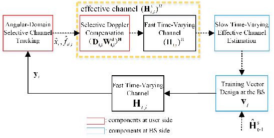
In this section, we propose an efficient angular-domain selective channel tracking and Doppler compensation scheme at the user side. The proposed scheme can exploit both dynamic sparsity of mmWave massive MIMO channel and high resolution of AoA at multi-antenna mobile users to accurately estimate the downlink AoAs and maximum DFO. Using these estimated parameters, a Doppler compensation matrix is applied at the user to convert the fast time-varying channel into a slow time-varying effective channel, based on which efficient downlink/uplink transmissions can be achieved. The proposed scheme includes four key components, namely the Angular-Domain Selective Channel Tracking, Selective Doppler Compensation, Slow Time-Varying Effective Channel Estimation, and Downlink Training Vector Design. Fig. 2 illustrates a top-level diagram of the proposed scheme and the details of each component are elaborated below. The frame index will be omitted when there is no ambiguity.
III-A Outline of Angular-Domain Selective Channel Tracking at the User
This component is used to estimate the downlink AoAs, rotation angle and maximum DFO based on the downlink training vectors. Thanks to the high-spatial resolution provided by the large array at the user side, the user can distinguish DFOs associated with different AOAs from multiple active paths. However, since both the BS and the user are equipped with the large array, the parameter space can be very large if we attempt to estimate the full angular–domain channel parameters (i.e., the full angular domain channel matrix , rotation angle and maximum DFO ). Since the DFO only occurs at the mobile user side, we propose to only estimate partial angular–domain channel parameters that are just sufficient to obtain AoAs, rotation angle and maximum DFO for Doppler compensation.
Specifically, the product of channel and downlink training vector can be expressed as:
| (3) |
where with are called partial angular channel coefficients since only contain partial information about the full angular channel . Specifically, a non-zero with value larger than the noise floor indicates that there is an active path to the -th AoA direction at the user side. Therefore, we only need to estimate partial channel parameters , the AoA off-grid vector , rotation angle and maximum DFO , which are much less than the original full channel parameters, the off-grid vector , rotation angle and maximum DFO. Note that if the training vectors are different, there will be partial angular channel coefficients, leading to a larger parameter space to be estimated. Moreover, with uniformly distributed training vectors, the phase rotation due to the Doppler term is larger compared to the case when the training vectors are squeezed in the beginning of the downlink subframe, leading to a better estimation performance for the Doppler parameter . Therefore, such a selective channel tracking design based on uniformly distributed and identical training vectors can significantly reduce the number of downlink training vectors required to achieve accurate estimation of AoAs, rotation angle and Doppler parameters.
The received baseband pilot signal is given by
| (4) |
where is the training vector for downlink channel tracking, and is the additive white Gaussian noise (AWGN) with each element having zero mean and variance , respectively. The exact choice of is postponed to Section III-D.
The aggregate received pilot signal (channel measurements) of all the downlink pilot symbols (training vectors) in the -th frame can be expressed in a compact form as
| (5) |
Based on the received downlink training vectors, the user obtains the estimated partial channel parameters , , and using a selective channel tracking algorithm. The detailed problem formulation and algorithm design for selective channel tracking scheme are postponed to Section IV.
III-B Angular-Domain Selective Doppler Compensation at the User
This component is used to convert the fast time-varying channel into a slow time-varying effective channel after obtaining the estimated partial channel parameters , , and . We first select a set of most significant AoA directions with the largest energy, where the energy of the -th AoA direction is defined as . The parameter is used to control the tradeoff between the spatial multiplexing gain and the effective CSI signaling overhead (i.e., the CSI signaling overhead required to obtain effective channel in (6)). Let denote the index set of the selected most significant AoA directions. Then, in order to mitigate the Doppler effect and perform per-AoA DFO compensation for each selected AoA direction, a DFO compensation matrix , which also serves as beamforming matrix, is applied at the user side. In this way, we can convert the fast time-varying channel into a slow time-varying effective channel as
| (6) |
where and .
In the following, we explain why the Doppler effect can be alleviated by applying the above DFO compensation matrix to obtain an effective channel . For half-wavelength space ULA, if there is no estimation error for the partial channel parameters, we have
| (7) |
as [27]. From (7), is constant within a frame if we ignore the small order term , i.e., the Doppler effect can be completely eliminated for sufficiently large . This observation is also consistent with the results in [18].
III-C Slow Time-Varying Effective Channel Estimation at the BS
The user can simply transmit orthogonal pilots in the uplink training stage. Then the conventional Least Squares (LS) based channel estimation method can be used at the BS to obtain the estimated slow time-varying effective channel . Based on , the BS can optimize the precoder for both uplink and downlink transmissions. Note that the optimization of MIMO precoder is a standard problem and there are many existing solutions with different performance and complexity tradeoff. Then, the optimized uplink precoder is fed back to the user for uplink transmission. Since can be much less than , the feedback overhead for the optimized uplink precoder is acceptable for practice.
III-D Training Vector Design at the BS
The training vector at the BS is designed according to the slow time-varying effective channel estimated at the end of the -th uplink subframe. The basic idea for training vector design is to strike a balance between exploitation of known channel directions (i.e., transmitting training signal over the most promising channel directions with large effective channel energy to achieve beamforming gain) and exploration of unknown channel directions (i.e., transmitting training signal over other channel directions to detect unknown channel directions). Since the effective channel changes slowly, the effective channel estimated at the end of the -th uplink subframe is expected to provide valuable information for the most promising channel directions. On the other hand, the information about the most promising channel directions extracted from may not be perfect due to the estimation error and CSI delay. In addition, some new direction may arise in the next frame. Therefore, the other channel directions should also be incorporated into the training vector to facilitate the detection of unknown channel directions.
Specifically, we first project the estimated effective channel onto an orthogonal basis to obtain the effective channel energy on each basis vector (quantized channel direction) as . The basis matrix is chosen such that the projection vector is as sparse as possible. For half-wavelength ULAs, we can simply choose the basis matrix as an DFT matrix. Then we find the index set of the most promising channel directions as
| (8) |
where is a threshold which is chosen to be closed to 1. In other words, the most promising channel directions contain fraction of the total effective channel energy. Let . Finally, the training vector is given by
| (9) |
where the first term in (9) exploites the information about the most promising channel directions extracted from , is a system parameter which determines the proportion of transmit power used to exploit the most promising channel directions, the second term is used to detect the other unknown channel directions, is randomly generated from .

In Fig. 3, we illustrate how the achievable data rate is affected by changing the parameters and to achieve different tradeoffs between the exploration and exploitation. It can be seen that setting and can strike a good balance between exploitation and exploration.
IV Problem Formulation for Angular-Domain Selective Channel Tracking
IV-A Three-layer Hierarchical Markov Model for Partial Angular Channel Vector
The dynamic sparsity of the partial angular channel coefficients is captured using a three-layer hierarchical Markov model, as illustrated in Fig. 4. The first layer of random variable is the channel support vector , whose -th element, denoted by , indicates whether the channel coefficient is active () or not (). The second layer of random variable is the precision vector , where represents the precision (inverse of the variance) of . The third layer of random variables are partial angular channel coefficients . For convenience, denote a time series of vectors as (same for , , ,). Then the three-layer hierarchical Markov prior distribution (joint distribution of , and ) is given by
| (10) |
where , the conditional probability has a product form and each is modeled as a Gaussian prior distribution
| (11) |
The conditional prior of precision vector is given by
| (12) |
is a Gamma hyperprior. are the shape and rate parameters of the channel precision conditioned on and they should be chosen such that , since the variance of is when it is active (). are the shape and rate parameters , conditioned on the opposite event (i.e., ). In this case, the shape and rate parameters of the precision should be chosen such that , since the variance of is close to zero when it is inactive.
Note that the exact channel distribution is usually unknown in practice. In this case, it is reasonable to choose a prior distribution such that the derived algorithm can promote sparsity with low complexity and achieve robust performance to different channel distributions. By controlling the parameters in the Gamma distribution of , one can easily promote sparsity based on the knowledge of channel support , as explained above. Moreover, Since the Gamma distribution for is the conjugate probability distribution of the Gaussian distribution for , the above hierarchical prior for and facilitates low-complexity VBI algorithm design with closed-form update equations [24]. Finally, the VBI-type algorithm derived from the such a hierarchical prior is well known to be insensitive to the true distribution of the sparse signals [24, 28]. As a result, similar hierarchical prior distribution has been widely adopted in sparse Bayesian learning [29].
Due to the slowly changing propagation environment, the channel supports often change slowly over time, which implies that depends on , e.g., if , then there is a higher probability that is also 1. Such dynamic sparsity of support vectors can be naturally modeled as a temporal Markov model with an initial prior distribution and a transition probability:
| (13) |
where the transition probability is given by , and . The Markov parameters characterize the degree of temporal correlation of the channel support. Specifically, smaller or lead to highly correlated supports across time, which means the propagation environment between the user and BS is changing slowly. Larger or can allow support to change substantially across time, which means the propagation environment is changing significantly. Moreover, the statistic parameters could be automatically learned based on the EM framework during the recovery process [30], as detailed in Appendix -A. The initial distribution is set to be the steady state distribution of the Markov chain in (13), i.e.,
This ensures that all elements of have the same marginal distribution .
In practice, the noise precision is usually unknown and we model it as a Gamma hyperpiror , where we set as in [25] so as to obtain a broad hyperprior.

IV-B Selective Channel Tracking Formulation
Using the angular domain channel representation, the receive signal at -th frame can be rewritten as a CS model with an unknown AoA off-grid and DFO parameter pair in the measurement matrix as
| (14) |
where the measurement matrix is given by , , .
In each frame , the user needs to estimate the partial channel parameters , the AoA off-grid and DFO parameter pair , given the observations up to frame in model (14), the estimated AoA off-grid and DFO parameter pairs up to frame. In particular, for given , we are interested in computing minimum mean-squared error (MMSE) estimates of , , where the expectation is over the marginal posterior:
| (15) |
where , denotes the vector collections integration over except for the element and denotes equality after scaling.
On the other hand, the optimal at the -th frame is obtained by ML as follows [25]:
| (16) |
Once we obtain the ML estimate of , and the associated conditional marginal posterior , we can obtain the MMSE estimates of .
One challenge in computing the MMSE estimate is the calculation of the exact posterior in (15) whose factor graph has loops. In the next subsection, we propose a Doppler-aware-dynamic-VBI (DD-VBI) algorithm to approximately calculate the marginal posteriors by combining the message passing and VBI approaches, and use the in-exact majorization-minimization (MM) method (which is a generalization of the EM method) [25] to find an approximate solution for (16). The proposed DD-VBI algorithm is shown in the simulations to achieve a good performance.
V Doppler-Aware-Dynamic-VBI algorithm
V-A Decomposition and Approximation of Joint Probability Distribution
This section is to decompose and approximate the joint probability distribution in (16) such that the joint probability distribution at the -th frame only involves the probability density function (PDF) of the current hidden variables , the current observation , and the messages passed from the previous frame, based on which a more efficient algorithm can be designed.
where , is a tractable approximation for the posterior and . Both and can be calculated based on the messages passed from the previous frame. We will elaborate how to calculate later in subsection V-E. When , is reduced to .
For simplicity, we define
| (17) |
In the rest of this section, we will omit in the PDFs when there is no ambiguity.
V-B Outline of the Doppler-Aware-Dynamic-VBI algorithm in Frame
The basic idea of the DD-VBI algorithm is that, at every frame , simultaneously approximates the marginal posterior and maximizes the log-likelihood with respect to , based on the noisy measurements of the -th frame and the messages passed from the previous frame. In summary, for every frame, the DD-VBI algorithm performs iterations between the following two major steps until convergence, as shown in Fig. 5.
- •
DD-VBI-E Step: Given at -th frame and messages passed from the previous frame, calculate the approximate marginal posterior of , denoted as , using the sparse VBI approach, as elaborated in subsection V-D.
- •
DD-VBI-M Step: Given , construct a surrogate function for the objective function , then maximize the surrogate function with respect to as elaborated in subsection V-C.
After convergence, the messages are calculated based on and passed to the next frame. In the following, we first elaborate the M step, which is a variation of the in-exact MM method in [25]. After that, we will elaborate how to approximately calculate the posterior in the E step, which is required to construct the surrogate function in the M step.

V-C DD-VBI-M Step
It is difficult to directly maximize the log-likelihood function , because there is no closed-form expression due to the multi-dimensional integration over as in (16). To make the problem tractable, in the DD-VBI-M Step, we adopt an in-exact MM method in [31, 25], which maximizes a surrogate function of with respect to , to find an approximate solution of (16). Specifically, let be the surrogate function constructed at some fixed point , which satisfies the following properties:
| (18) |
Inspired by the EM algorithm [31], we use the following surrogate function:
| (19) |
where is a tractable approximation of . In subsection V-A, we have approximated the joint probability distribution in (19) using . Therefore, the surrogate function can be approximated as
| (20) |
When there is no approximation error for the associated PDFs, i.e., and , it can be verified that satisfies the properties in (18).
In the M step of the -th iteration, we update as
| (21) |
where stands for the -th iteration.
In our problem, is a non-convex function and it is difficult to find its optimal solution. Therefore, we use a simple gradient update as in [25], i.e.
| (22) |
where is the step sizes determined by the Armijo rule [25].
The approximate posterior has a factorized form as
| (23) |
Therefore, after the convergence of the DD-VBI, we not only obtain an approximate stationary solution of (16), but also the associated (approximate) marginal conditional posterior .
V-D DD-VBI-E Step
DD-VBI-E Step performs the sparse VBI to approximate the conditional marginal posteriors based on the following joint prior distribution:
| (24) |
The corresponding approximate posterior distributions obtained by the sparse VBI will be given by (30)-(37).
V-D1 Outline of Sparse VBI within a Frame
For convenience, we use to denote an individual variable in . Let . Moreover, we use as a simplified notation for when there is no ambiguity. The approximate conditional marginal posterior could be calculated by minimizing the Kullback-Leibler divergence (KLD) between and subject to a factorized form constraint on as
| (25) | ||||
| (26) | ||||
| (27) |
Problem is non-convex, we aim at finding a stationary solution (denoted by ) of , as defined below.
Definition 1.
[Stationary Solution] is called a stationary solution of Problem if it satisfies all the constraints in and ,
By finding a stationary solution of , we could obtain the approximate posterior .
A stationary solution of can be obtained via alternately optimizing each individual density . For given , the optimal that minimizes the KLD in is given by
| (28) |
where . However, is intractable. Since in (17), (28) can be approximated as
| (29) |
Based on (29), the update equations of all variables are given in the subsequent subsections. The detailed derivation can be found in Appendix -B. Note that the operator is equivalent to and the expectation w.r.t. its own approximate posterior is simplified as .
V-D2 Initialization of Sparse VBI
In order to trigger the alternating optimization (AO) algorithm, we use the following initializations for the distribution functions in the first iteration of every frame and in the first iteration of first frame. In the rest iterations, we initialize ,, to the (approximate) posterior calculated in the previous frame.
- •
Initialize with .
- •
For given , initialize a gamma distribution for : , where , .
- •
Initialize a Gaussian distribution for : , where
V-D3 Update for
V-D4 Update for
can be derived as
| (31) |
and can be calculated through
| (32) |
| (33) |
where , , , .
V-D5 Update for
can be derived as
| (34) |
where are given by:
| (35) | ||||
| (36) |
where , is the -th element of , is the -th diagonal element of .
V-D6 Update for
can be derived as
| (37) |
where is given by
| (38) |
and is the normalization constant, given by , , is the digamma function, defined as the logarithmic derivative of the gamma function.
1: for do
2: Initialize the distribution functions according to Section
V-D2.
3: while not converge do
4: while not converge do
5: %DD-VBI-E Step:
6: Update using (30).
7: Update using (31).
8: Update using (34).
9: Update using (37) .
10: end while
11: %DD-VBI-M Step:
12: Construct the surrogate function in (20) using the
output of DD-VBI-E Step
13: Update using (21).
14: end while
15: Let denote the converged maximum DFO for frame
. Calculate using (40).
Pass messages to frame .
16: Estimate using (33).
17: end for
V-E Messages Passed to the Next Frame
After the convergence of the DD-VBI iterations in frame , let and denote the converged Doppler parameter and the associated approximate posterior for , respectively. Then, the messages is calculated as
| (39) | ||||
| (40) |
where
Finally, the messages , as the prior to the channel support, is passed to the next frame.
The overall DD-VBI algorithm is summarized in Algorithm 1. Note that in the -th frame of DD-VBI, the contribution of the previous observations on the estimation of and is summarized in the messages passed from frame . Therefore, in the -th frame, there is no need to store all the observations up to frame .
Remark 2.
In practical mmWave massive MIMO systems, the number of RF chains can be less than the number of antennas at both the BS and user sides to reduce the hardware cost and power consumption. The proposed scheme can be easily extended to the case with limited RF chains. For example, suppose there are only RF chains at the BS and RF chains at the user. In this case, when the BS transmits the training vector for downlink channel tracking in the -th symbol duration, the user employs as a combining matrix to combine the received signal into baseband channel measurements, where and are the RF training matrix and baseband training vector at the BS, respectively, and and are the RF and baseband combining matrix at the mobile user in the -th symbol duration, respectively. We can still write the received pilot signal as a CS model as in (14), but with , , .
V-F Complexity and Signaling Overhead Comparison
The computational complexity of the proposed algorithm is dominated by the update of . Assuming the arithmetic with individual elements has complexity , the computational complexity of matrix inversion in (32) is and the total number of multiplications to update is . Supposing the algorithm executes iterations, the total complexity order of the proposed method is , considering that is usually larger than . In Table II and III, we assume the mmWave channel has dominant paths and compare the complexity and signaling overhead of the proposed algorithm with the following baseline algorithms:
- •
- •
- •
As seen from Table II, the complexity order of the proposed algorithm is similar to the baselines. For example, can range from to to achieve different tradeoff between performance and complexity, and we usually have , . For a resolution of the HS scheme, we usually have [21]. In this typical case, the complexity of the proposed scheme and the baseline schemes are shown in the third column of Table II. On the other hand, the proposed algorithm has the lowest signaling overhead for both the general case and the typical case, as shown in Table III.
| Algorithms | Complexity order | Typical complexity order |
|---|---|---|
| proposed | ||
| ML | ||
| ES | ||
| HS |
| Algorithms | Signaling overhead | Typical signaling overhead |
|---|---|---|
| proposed | ||
| ML | ||
| HS | ||
| ES |
VI Simulation Results
In this section, we compare the performance of the proposed algorithm with the baseline algorithms described in Section V-F. For the ML baseline, we also consider the case when only partial channel parameters are estimated as in the proposed scheme (ML-Partial). For the proposed scheme, we also consider the case when the training vector is generated randomly (DD-VBI-Random). The channel parameters are based on the millimeter-wave statistical spatial channel model (mm-SSCM) as specified in [32], which was developed according to the 28- and 73-GHz ultrawideband propagation measurements in New York City. The signal bandwidth is and the frame duration is set as . The carrier frequency is 28GHz . The mobile user employs a ULA of antennas and the inter antenna spacing is , and the BS also employs a ULA. The user velocity is assumed to be 380km/h, which translates to KHz.
In the simulation, we will consider both cases when the user is equipped with a full set of RF chains and limited RF chains. For the case with limited RF chains, the number of RF chains is set to be . The MSE for DFO estimation and the uplink achievable data rate are adopted as the performance metrics. The frequency MSE and the channel MSE is defined as and , respectively. The parameter is chosen to be equal to the number of dominant AoA directions at the user side (an AoA direction is called a dominant AoA direction if its energy is no less than 10% of the most significant AoA direction) and data streams are transmitted over the dominant AoA directions in the uplink with equal power allocation. Since the uplink transmission is only designed based on the dominant AoA directions which are known at the user, there is no need for the BS to feed back the slow time-varying effective channel.
VI-A Doppler Frequency and Channel MSE Performance

The Doppler frequency and channel MSE performance of different algorithms versus the pilot number, SNR and number of BS antennas are shown in Fig. 6 and Fig. 7. It can be seen that the proposed DD-VBI algorithm achieves large performance gain over all the baseline algorithms, under both full RF chains and limited RF chains. By using the proposed training vector design to strike a balance between exploitation of known channel directions and exploration of unknown channel directions, the DD-VBI algorithm could further improve the MSE performance compared to the case with a random training vector. This demonstrates that the proposed algorithm can effectively estimate the maximum DFO by selective channel tracking and efficient training vector design. Note that as the number of BS antennas increases, the parameters to be estimated increase significantly and the spatial resolution and array gain will also increase. Since the ML-Full method does not exploit the selective channel estimation method or channel sparsity to reduce the number of free parameters, its performance may degrade with the number of BS antennas. However, the performance gain of the proposed algorithm improves because in this case, the number of parameters to be estimated does not increase with the number of BS antennas. This demonstrates that the proposed algorithm is a powerful method for accurate DFO estimation, even when both BS and mobile user are equipped with massive MIMO, and the number of RF chains at the user side is limited.

VI-B Achievable Data Rate Performance

The achievable data rates of different algorithms versus the pilot number, SNR and number of BS antennas are shown in Fig. 8. It can be observed that the performance of all algorithms increases with the number of pilots, SNR and number of BS antennas. The proposed DD-VBI algorithm can achieve large performance gain over various baselines under both full RF chains and limited RF chains. Moreover, by using the proposed training vector design, the proposed DD-VBI algorithm could further improve the achievable data rate. This verifies that the proposed selective channel tracking and Doppler compensation scheme can also enhance the achievable data rate with low pilot overhead, under different SNRs and numbers of BS antennas.
VI-C Complexity versus Realized Gain
In practice, we can control the tradeoff between the complexity and realized gain of the proposed algorithm by adjusting the number of iterations. In Fig. 9, we plot the achievable rate versus the CPU time. It can be seen that the proposed algorithm can achieve a better performance than the baseline algorithms for the same CPU time. Moreover, the performance gain increases with the CPU time. Therefore, the proposed algorithm provides a better and more flexible tradeoff between the performance and computational power.

VII Conclusion
We propose an angular-domain selective channel tracking and Doppler compensation scheme for high-mobility massive MIMO systems. Firstly, we propose a selective channel tracking scheme and the associated Doppler-aware-dynamic-VBI algorithm to accurately estimate the DFO and partial angular–domain channel parameters with reduced pilot overhead. Then, we propose an angular-domain selective DFO compensation scheme to convert the dominant paths of the fast time-varying channel into a slow time-varying effective channel, based on which efficient uplink and downlink transmissions can be achieved. Simulations verify that the proposed scheme not only can mitigate the Doppler and channel aging effect with much less pilots than existing schemes, but also can achieve a good tradeoff between the CSI signaling overhead and spatial multiplexing/array gain.
-A EM Estimation of the Parameters and
Denote the as the channel support vector, as defined in SubSec.IV-A. We apply the EM method in [31] to obtain an estimate of the parameter by perform the following iterations until convergence:
| (41) |
where stands for the -th iteration, denotes expectation over the posterior distribution conditioned on and . Solving the problem (41), we can get a closed-form expression for updating the as
| (42) |
Since the channel support vector forms a Markov chain, the posterior distribution can be approximately calculated using the sum-product message passing over the factor graph of the associated Markov chain with the priors of ’s given by the output of the DD-VBI algorithm at each frame [30]. After the iterations in (42) convergence, we can obtain the EM estimation of the parameter in the t-th frame. The EM estimation of the parameter can be obtained in a similar way.
-B Derivation of (30)-(37)
References
- [1] M. Souden, S. Affes, J. Benesty, and R. Bahroun, “Robust Doppler Spread Estimation in the Presence of a Residual Carrier Frequency Offset,” IEEE Transactions on Signal Processing, vol. 57, no. 10, pp. 4148–4153, 2009.
- [2] C. R. Berger, Z. Wang, J. Huang, and S. Zhou, “Application of compressive sensing to sparse channel estimation,” IEEE Communications Magazine, vol. 48, no. 11, pp. 164–174, 2010.
- [3] X. Wang, G. Wang, R. Fan, and B. Ai, “Channel Estimation with Expectation Maximization and Historical Information based Basis Expansion Model for Wireless Communication Systems on High Speed Railways,” IEEE Access, vol. 6, no. 99, pp. 72–80, 2018.
- [4] Y. Mostofi and D. C. Cox, “ICI Mitigation for Pilot-aided OFDM Mobile Systems,” IEEE Transactions on Wireless Communications, vol. 4, no. 2, pp. 765–774, 2005.
- [5] T. L. Liu, W. H. Chung, S. Y. Yuan, and S. Y. Kuo, “On the Banded Approximation of the Channel Matrix for Mobile OFDM Systems,” Vehicular Technology IEEE Transactions on, vol. 64, no. 8, pp. 3526–3535, 2015.
- [6] W. Xin, X. X. Yang, and Y. Z. Wang, “Study on Channel Estimation in Time-Varing Amplify and Forward Relay Networks,” Applied Mechanics Materials, vol. 519-520, pp. 934–938, 2014.
- [7] T. Y. Al-Naffouri, K. M. Z. Islam, N. Al-Dhahir, and S. Lu, “A Model Reduction Approach for OFDM Channel Estimation Under High Mobility Conditions,” IEEE Transactions on Signal Processing, vol. 58, no. 4, pp. 2181–2193, 2010.
- [8] Y. Ge, W. Zhang, F. Gao, and H. Minn, “Angle-Domain Approach for Parameter Estimation in High-Mobility OFDM with Fully/Partly Calibrated Massive ULA,” IEEE Transactions on Wireless Communications, pp. 1–1, 2018.
- [9] A. Monk, R. Hadani, M. Tsatsanis, and S. Rakib, “OTFS-Orthogonal Time Frequency Space,” 2016.
- [10] M. K. Ramachandran and A. Chockalingam, “MIMO-OTFS in High-Doppler Fading Channels: Signal Detection and Channel Estimation,” 2018.
- [11] F. Bellili and S. Affes, “A Low-cost and Robust Maximum Likelihood Doppler Spread Estimator,” in Global Communications Conference, 2014, pp. 4325–4330.
- [12] D. Chizhik, “Slowing the Time-fluctuating MIMO Channel,” IEEE Transactions on Wireless Communications, vol. 3, no. 5, pp. 1554–1565, 2004.
- [13] Y. Zhang, Q. Yin, P. Mu, and L. Bai, “Multiple Doppler Shifts Compensation and ICI Elimination by Beamforming in High-mobility OFDM systems,” in International ICST Conference on Communications and NETWORKING in China, 2012, pp. 170–175.
- [14] W. Guo, P. Mu, Q. Yin, and H. M. Wang, “Multiple Doppler frequency offsets compensation technique for high-mobility OFDM uplink,” in IEEE International Conference on Signal Processing, Communication and Computing, 2013, pp. 1–5.
- [15] Z. Liu, J. Wu, and P. Fan, “On the Uplink Capacity of High Speed Railway Communications with Massive MIMO Systems,” in Vehicular Technology Conference, 2014, pp. 1–5.
- [16] X. Chen, J. Lu, T. Li, P. Fan, and K. B. Letaief, “Directivity-Beamwidth Tradeoff of Massive MIMO Uplink Beamforming for High Speed Train Communication,” IEEE Access, vol. PP, no. 99, pp. 1–1, 2017.
- [17] W. Guo, W. Zhang, P. Mu, and F. Gao, “High-Mobility OFDM Downlink Transmission with Large-Scale Antenna Array,” IEEE Transactions on Vehicular Technology, vol. PP, no. 99, pp. 1–1, 2017.
- [18] W. Guo, W. Zhang, P. Mu, F. Gao, and H. Lin, “High-Mobility Wideband Massive MIMO Communications: Doppler Compensation, Analysis and Scaling Law,” 2018.
- [19] W. Guo, W. Zhang, P. Mu, F. Gao, and B. Yao, “Angle-Domain Doppler Pre-Compensation for High-Mobility OFDM Uplink with Massive ULA,” in GLOBECOM 2017 - 2017 IEEE Global Communications Conference, 2018, pp. 1–6.
- [20] J. Wang, L. Zhou, C. W. Pyo, T. Baykas, and S. Kato, “Beam Codebook Based Beamforming Protocol for Multi-Gbps Millimeter-Wave WPAN Systems,” IEEE Journal on Selected Areas in Communications, vol. 27, no. 8, pp. 1390–1399, 2009.
- [21] A. Alkhateeb, O. E. Ayach, G. Leus, and R. W. H. Jr, “Channel Estimation and Hybrid Precoding for Millimeter Wave Cellular Systems,” IEEE Journal of Selected Topics in Signal Processing, vol. 8, no. 5, pp. 831–846, 2017.
- [22] Z. Gao, L. Dai, H. Chen, and Z. Wang, “Channel Estimation for Millimeter-Wave Massive MIMO with Hybrid Precoding over Frequency-Selective Fading Channels,” IEEE Communications Letters, vol. 20, no. 6, pp. 1259–1262, 2016.
- [23] W. U. Bajwa, J. Haupt, A. M. Sayeed, and R. Nowak, “Compressed Channel Sensing: A New Approach to Estimating Sparse Multipath Channels,” Proceedings of the IEEE, vol. 98, no. 6, pp. 1058–1076, 2010.
- [24] D. G. Tzikas, C. L. Likas, and N. P. Galatsanos, “The Variational Approximation for Bayesian Inference,” IEEE Signal Processing Magazine, vol. 25, no. 6, pp. 131–146, 2008.
- [25] J. Dai, A. Liu, and V. K. N. Lau, “Fdd massive mimo channel estimation with arbitrary 2d-array geometry,” IEEE Transactions on Signal Processing, vol. PP, no. 99, 2018.
- [26] C. B. Dietrich, “Adaptive Arrays and Diversity Antenna Configurations for Handheld Wireless Communication Terminals,” Dissertation Abstracts International, Volume: 63-08, Section: B, page: 3841.;Chair: Warren L. Stutz, 2000.
- [27] A. Adhikary, J. Nam, J.-Y. Ahn, and G. Caire, “Joint Spatial Division and Multiplexing - The Large-Scale Array Regime,” vol. 59, no. 10, pp. 6441–6463, Oct. 2013.
- [28] S. Ji, Y. Xue, and L. Carin, “Bayesian Compressive Sensing,” IEEE Transactions on Signal Processing, vol. 56, no. 6, pp. 2346–2356, 2008.
- [29] D. P. Wipf and B. D. Rao, “Bayesian Learning for Sparse Signal Reconstruction,” in IEEE International Conference on Acoustics, 2003.
- [30] J. Ziniel and P. Schniter, “Dynamic Compressive Sensing of Time-Varying Signals via Approximate Message Passing,” IEEE Transactions on Signal Processing, vol. 61, no. 21, pp. 5270–5284, 2013.
- [31] A. P. Dempster, “Maximum Likelihood Estimation from Incomplete Data via the EM Algorithm,” Journal of the Royal Statistical Society, vol. 39, no. 1, pp. 1–38, 1977.
- [32] M. K. Samimi and T. S. Rappaport, “3-D Millimeter-Wave Statistical Channel Model for 5G Wireless System Design,” IEEE Transactions on Microwave Theory Techniques, vol. 64, no. 7, pp. 1–19, 2016.