跳到论文正文
W Papers独立论文阅读器 arXiv:1911.08526 论文正文 计算阅读时间 · 0%
引用这篇论文根据当前论文元数据生成,正式投稿前建议核对。


License: arXiv.org perpetual non-exclusive license
arXiv:1911.08526v1 [math.OC] 19 Nov 2019

The nonsmooth landscape of blind deconvolution

Mateo Díaz Thanks: people.cam.cornell.edu/md825/ Affiliation: Center for Applied Mathematics Affiliation: Cornell University
Abstract

The blind deconvolution problem aims to recover a rank-one matrix from a set of rank-one linear measurements. Recently, Charisopulos et al. [1] introduced a nonconvex nonsmooth formulation that can be used, in combination with an initialization procedure, to provably solve this problem under standard statistical assumptions. In practice, however, initialization is unnecessary. As we demonstrate numerically, a randomly initialized subgradient method consistently solves the problem. In pursuit of a better understanding of this phenomenon, we study the random landscape of this formulation. We characterize in closed form the landscape of the population objective and describe the approximate location of the stationary points of the sample objective. In particular, we show that the set of spurious critical points lies close to a codimension two subspace. In doing this, we develop tools for studying the landscape of a broader family of singular value functions, these results may be of independent interest.

1 Introduction

An increasing amount of research has shown how matrix recovery problems, which in the worst case are hard, become tractable under appropriate statistical assumptions. Examples include phase retrieval [2, 3, 4], blind deconvolution [5, 1], matrix sensing [6, 7], matrix completion [8, 9], and robust PCA [10, 11], among others [12, 13, 14, 15]. Convex relaxations have proven to be a great tool to tackle these problems, but they often require lifting the problem to a higher dimensional space and consequently end up being computationally expensive. Thus, focus has shifted back to iterative methods for nonconvex formulations that operate in the natural parameter space. One of the difficulties of nonconvex optimization is that, in general, it is hard to find global minimizers. To overcome this issue, recent works have suggested two stage methods: One starts by running an initialization procedure – usually based on spectral techniques – and then refines the solution by warm-starting a local search method that minimizes a nonconvex formulation. This thread of ideas has proven very successful, and we refer the reader to [16] for a survey.

Initialization procedures are nontrivial to develop and can sometimes more expensive than the refinement stage. Thus, it is important to understand when initialization methods are superfluous. There are iterative methods, for specific problems, that provably converge to minimizers [9, 17, 12, 18, 19]. Analysis of these methods are of two types: those based on studying the iterate sequence [20, 21, 22], and those based on characterizing the landscape of smooth loss functions [17, 23, 24].

In this work, we study the landscape of a nonsmooth nonconvex formulation (2) for the (real) blind deconvolution problem. Unlike the aforementioned works, we consider a nonsmooth loss, which presents fundamentally different technical challenges. We show that, as the number of measurements grow, the set of spurious stationary points converges to a codimension two subspace. This suggests that there is an extensive region with friendly geometry.

The blind deconvolution problem aims to recover a pair of real vectors (w¯,x¯)∈ℝd1×ℝd2(\bar{w},\bar{x})\in\mathbb{R}^{d_{1}}\times\mathbb{R}^{d_{2}} from a set of mm observations given by

yi=⟨ai,w¯⟩​⟨x¯,bi⟩for all ​i∈1,…,my_{i}=\langle a_{i},\bar{w}\rangle\langle\bar{x},b_{i}\rangle\qquad\text{for all }i\in{1,\dots,m} (1)

where aia_{i} and bib_{i} are known vectors for all indices. This problem has important applications in a variety of different fields, we describe two below.

  1. Signal processing. The complex analogue of this problem is intimately linked to the problem of recovering a pair of vectors (u,v)(u,v) from the convolution (A​u)∗(B​v)(Au)\ast(Bv), where AA and BB are tall-skinny matrices. In fact, when passed to the frequency domain, this problem becomes equivalent to the one mentioned above. This problem has applications in image deblurring and channel protection with random codes [25, 23].

  2. Shallow neural networks. Solving this problem is equivalent to learning the weights of a shallow neural network with bilinear activation functions. Taking {((ai,bi),yi)}\big\{((a_{i},b_{i}),y_{i})\big\} as training data, writing the output of the network as y=σ⁡(a⊤​w,b⊤​x)y=\sigma(a^{\top}w,b^{\top}x), with (w,x)∈ℝd1×d2(w,x)\in\mathbb{R}^{d_{1}\times d_{2}}, and the setting the activation function to σ⁡(z1,z2)=z1​z2.\sigma(z_{1},z_{2})=z_{1}z_{2}.

To tackle the blind deconvolution problem, [1] proposed the following nonconvex nonsmooth formulation

argminw,xfS​(w,x)≜1m​∑i=1m|⟨ai,w⟩​⟨x,bi⟩−yi|.\operatornamewithlimits{argmin}_{w,x}f_{S}(w,x)\triangleq\frac{1}{m}\sum_{i=1}^{m}|\langle a_{i},w\rangle\langle x,b_{i}\rangle-y_{i}|. (2)

The authors of [1] designed a two-stage method based on this formulation and showed that if the measuring vectors, aia_{i} and bi,b_{i}, are i.i.d standard Gaussian, then their algorithm converges rapidly to a solution whenever m≳(d1+d2).m\gtrsim(d_{1}+d_{2}). 11 1 This is information-theoretically optimal up to constants [26, 27]. Nonetheless, experimentally the initialization stage seems to be superfluous. Indeed, a simple randomly-initialized subgradient algorithm is successful at solving the problem most of the time provided that m/(d1+d2)m/(d_{1}+d_{2}) is big enough, see the experiments in the last section for support of this claim.

1.1 Main contributions

Aiming to get a better understanding of the high-dimensional geometry of fSf_{S}, we study the landscape of fSf_{S} when AA and BB are standard Gaussian random matrices. Following the line of ideas in [28], we think of fSf_{S} as the empirical average approximation of the population objective

fP​(w,x)≜𝔼​fS​(w,x)=𝔼⁡(|a⊤​(w​x−w¯​x¯)​b⊤|),f_{P}(w,x)\triangleq\mathbb{E}f_{S}(w,x)=\mathbb{E}\left(|a^{\top}(wx-\bar{w}\bar{x})b^{\top}|\right),

where a∈ℝd1a\in\mathbb{R}^{d_{1}} and b∈ℝd2b\in\mathbb{R}^{d_{2}} are standard Gaussian vectors. From now on, we will refer to fSf_{S} as the sample objective. The rationale is simple: we will describe the stationary points of fPf_{P}, then we will prove that the graph of the subdifferential ∂fS\partial f_{S} concentrates around the graph of ∂fP\partial f_{P} and combine these to describe the landscape of fS.f_{S}.22 2 We will give a formal definition of ∂f\partial f in Section 2. This strategy allows us to show that the set of spurious stationary points converges to a codimension two subspace at a controlled rate. We remark that these results are geometrical and not computational.

Before we go on, let us observe that one can only wish to recover the pair (w¯,x¯)(\bar{w},\bar{x}) up to scaling. In fact, the measurements (1) are invariant under the mapping (w,x)↦(α​w,x/α)(w,x)\mapsto(\alpha w,x/\alpha) for any α≠0.\alpha\neq 0. Hence the set of solutions of the problems is defined as

𝒮≜{(α​w¯,x¯/α)∣α∈ℝ∖{0}}.\mathcal{S}\triangleq\left\{\left(\alpha\bar{w},\bar{x}/\alpha\right)\mid\alpha\in\mathbb{R}\setminus\{0\}\right\}.

Population objective.

Interestingly, the population objective only depends on (w,x)(w,x) through the singular values of the rank two matrix X:=w​x⊤−w¯​x¯⊤.X:=wx^{\top}-\bar{w}\bar{x}^{\top}. We show this function can be written as

fP​(w,x)=σmax​(X)​∑n=0∞((2​n)!22​n​(n!)2)2​(1−κ−2​(X))n1−2​nf_{P}(w,x)=\sigma_{\max}(X)\sum_{n=0}^{\infty}\left(\frac{(2n)!}{2^{2n}(n!)^{2}}\right)^{2}\frac{\left(1-\kappa^{-2}(X)\right)^{n}}{1-2n}

where κ⁡(X)=σmax​(X)/σmin​(X)\kappa(X)={\sigma_{\max}(X)}/{\sigma_{\min}(X)} is the condition number of X.X. We characterize the stationary points of a broad family of spectral functions, containing fPf_{P}. By specializing this characterization we find that the stationary points of the population objectives are exactly

𝒮∪{(w,x)∣⟨w,w¯⟩=0,⟨x,x¯⟩=0,and wx⊤=0},\mathcal{S}\cup\{(w,x)\mid\langle w,\bar{w}\rangle=0,\langle x,\bar{x}\rangle=0,\text{and }wx^{\top}=0\},

revealing that the set of extraneous critical points of fPf_{P} is the subspace (w¯,0)⟂∩(0,x¯)⟂.(\bar{w},0)^{\perp}\cap(0,\bar{x})^{\perp}.

Sample objective.

Equipped with a quantitative version of Attouch-Wets’ convergence theorem proved in [28], we show that with high probability any stationary point of fSf_{S} in a bounded set satisfies at least one of the following

∥(w,x)∥≤Δ∥(w¯,x¯)∥,∥wx⊤−w¯x¯⊤∥≤Δ∥w¯x¯⊤∥,or{|⟨w,w¯⟩|≤Δ​‖(w,x)‖​‖w¯‖,|⟨x,x¯⟩|≤Δ​‖(w,x)‖​‖x¯‖.\|(w,x)\|\leq\Delta\|(\bar{w},\bar{x})\|,\;\;\|wx^{\top}-\bar{w}\bar{x}^{\top}\|\leq\Delta\|\bar{w}\bar{x}^{\top}\|,\;\;\text{or}\;\;\left\{\begin{array}[]{ll}|\langle w,\bar{w}\rangle|&\leq\Delta\|(w,x)\|\|\bar{w}\|,\\ |\langle x,\bar{x}\rangle|&\leq\Delta\|(w,x)\|\|\bar{x}\|.\end{array}\right.

provided that m≳d1+d2,m\gtrsim d_{1}+d_{2}, where Δ=𝒪~​(d1+d2m)18\Delta=\widetilde{\mathcal{O}}\left(\frac{d_{1}+d_{2}}{m}\right)^{\frac{1}{8}}.33 3 Where 𝒪~\widetilde{\mathcal{O}} hides logarithmic terms. Intuitively this means, that as the ratio (d1+d2)/m(d_{1}+d_{2})/m goes to zero, the stationary points lie closer and closer to three sets: the singleton zero, the set of solutions 𝒮\mathcal{S}, and the subspace (w¯,0)⟂∩(0,x¯)⟂.(\bar{w},0)^{\perp}\cap(0,\bar{x})^{\perp}.

1.2 Related work

There is a vast recent literature on blind deconvolution. A variety of algorithmic solutions have been proposed, including convex relaxations [25, 29], Riemannian optimization methods [30], gradient descent algorithms [5, 31], and nonsmooth procedures [1]. Related to this work, the authors of [32, 33] studied variations of the blind deconvolution problem via landscape analysis; their approach is based on smooth formulations and therefore their tools are of a different nature. Besides algorithms, researchers have also been interested in information-theoretical limits of the problem under different assumptions[26, 34, 27].

On the other hand, the study of the high-dimensional landscape of nonconvex formulations is an emergent area of research. Examples for smooth formulations include the analysis for phase retrieval [23], matrix completion [9], robust PCA [17], and synchronization networks [24]. The majority of these results focus on using second order information to show that under reasonable assumptions the formulations do not exhibit spurious stationary points. The machinery developed for nonsmooth formulations is based on different ideas and is more case-oriented. Despite there are remarkable examples [28, 35, 36, 37]. Closer to our work is the paper [28]; the authors of this article studied a similar nonsmooth formulation for the phase retrieval problem, which can be regarded as a symmetric analogue of blind deconvolution.

1.3 Outline

The agenda of this paper is as follows: Section 2 introduces notation and some basic results we require. Sections 3 and 4 present the results on the landscape of the population and sample objectives, respectively. In Section 5, we present computational experiments corroborating the conclusions of our theory. We close with a brief discussion and future research directions in Section 6. Many of the arguments are technical and consequently we defer most of the proofs to the appendices.

2 Preliminaries

We will follow standard notation. The symbols ℝ\mathbb{R} and ℝ+\mathbb{R}_{+} denote the real line and the nonnegative reals, respectively. The set of extended reals ℝ∪{+∞}\mathbb{R}\cup\{+\infty\} is written as ℝ¯.\overline{\mathbb{R}}. We always endow ℝd\mathbb{R}^{d} with its standard inner product, ⟨x,y⟩=x⊤​y\langle x,y\rangle=x^{\top}y, and its induced norm ‖x‖=⟨x,x⟩\|x\|=\sqrt{\langle x,x\rangle}. We also use ‖x‖1=∑|xi|\|x\|_{1}=\sum|x_{i}| to denote the ℓ1\ell_{1}-norm. For a set S⊆ℝdS\subseteq\mathbb{R}^{d}, we denote the distance from a point xx to the set by dist⁡(x,Q)=infy∈Q‖x−y‖{\rm dist}(x,Q)=\inf_{y\in Q}\|x-y\|. For any pair of real-valued functions f,g:ℝn→ℝf,g:\mathbb{R}^{n}\rightarrow\mathbb{R}, we say that f≲gf\lesssim g if there exists a constant CC such that f≤C​g.f\leq Cg. Moreover, we write f≍gf\asymp g if both f≲gf\lesssim g and g≲f.g\lesssim f.

The adjoint of a linear operator A:ℝd→ℝnA:\mathbb{R}^{d}\rightarrow\mathbb{R}^{n} is indicated by A⊤:ℝn→ℝd.A^{\top}:\mathbb{R}^{n}\rightarrow\mathbb{R}^{d}. Assuming d≤nd\leq n, the map σ:ℝn×d→ℝ+d\sigma:\mathbb{R}^{n\times d}\rightarrow\mathbb{R}^{d}_{+} returns the vector of ordered singular values of a matrix with σ1​(A)≥σ2​(A)≥⋯≥σd​(A)\sigma_{1}(A)\geq\sigma_{2}(A)\geq\dots\geq\sigma_{d}(A). We will use the symbols ‖A‖op=σ1​(A)\|A\|_{\mathrm{op}}=\sigma_{1}(A) and ‖A‖F=‖σ⁡(A)‖2\|A\|_{F}=\|\sigma(A)\|_{2} to indicate the operator and Frobenius norm, respectively. When not specified it is understood that ‖A‖:=‖A‖op.\|A\|:=\|A\|_{\mathrm{op}}. We will use the symbol O⁡(d)O(d) to denote the set of d×dd\times d orthogonal matrix.

Variational analysis.

Since we will handle nonsmooth functions, we need a definition of generalized derivatives. We refer the interested reader to some excellent references on the subject [38, 39, 40]. Let f:ℝd→ℝ¯f:\mathbb{R}^{d}\rightarrow\overline{\mathbb{R}} be a lower semicontinuous proper function and x¯\bar{x} be a point. The Fréchet subdifferential ∂^​f​(x)\widehat{\partial}f(x) is the set of all vectors ξ\xi for which

f⁡(x)≥f⁡(x¯)+⟨ξ,x−x¯⟩+o⁡(‖x−x¯‖)as ​x→x¯.f(x)\geq f(\bar{x})+\langle\xi,x-\bar{x}\rangle+o(\|x-\bar{x}\|)\qquad\text{as }x\rightarrow\bar{x}.

Intuitively, ξ∈∂f⁡(x¯)\xi\in\partial f(\bar{x}) if the function x↦f⁡(x¯)+⟨ξ,x−x¯⟩x\mapsto f(\bar{x})+\langle\xi,x-\bar{x}\rangle locally minorizes ff up to first order information. Unfortunately, the set-valued mapping x↦∂^​f​(x)x\mapsto\widehat{\partial}f(x) lacks some desirable topological properties. For this reason it is useful to consider an extension. The limiting subdifferential ∂f⁡(x¯)\partial f(\bar{x}) is the set of all ξ\xi such that there are sequences (xn)(x_{n}) and (ξn)(\xi_{n}) with ξn∈∂^​f​(xn)\xi_{n}\in\widehat{\partial}f(x_{n}) satisfying (xn,f⁡(xn),ξn)→(x¯,f⁡(x¯),ξ)(x_{n},f(x_{n}),\xi_{n})\rightarrow(\bar{x},f(\bar{x}),\xi). It is well-known that ∂f⁡(x¯)\partial f(\bar{x}) reduces to the classical derivative when ff is Fréchet differentiable and that for ff convex, ∂f⁡(x¯)\partial f(\bar{x}) is equal to the usual convex subdifferential

ξ∈∂f(x¯)⇔f(x)≥f(x¯)+⟨ξ,x−x¯⟩∀x.\xi\in\partial f(\bar{x})\qquad\iff\qquad f(x)\geq f(\bar{x})+\langle\xi,x-\bar{x}\rangle\;\;\;\forall x.

We say that a point x¯\bar{x} is stationary if 0∈∂f⁡(x¯).0\in\partial f(\bar{x}). The graph of ∂f\partial f is given by gph​∂f={(x,ζ)∣ζ∈∂f⁡(x)}.{\rm gph}\,\partial f=\{(x,\zeta)\mid\zeta\in\partial f(x)\}.

For ρ>0,\rho>0, we say that ff is ρ\rho-weakly convex if the regularized function f+ρ2∥⋅∥22f+\frac{\rho}{2}\|\cdot\|^{2}_{2} is convex. This encompasses a broad class of functions: Any function that can be decomposed as f=h∘gf=h\circ g, where h:ℝm→ℝh:\mathbb{R}^{m}\rightarrow\mathbb{R} is a Lipschitz convex function and g:ℝd→ℝmg:\mathbb{R}^{d}\rightarrow\mathbb{R}^{m} is smooth map, is weakly convex. It is worth noting that for functions that can be decomposed in this fashion, the chain rule [38, Theorem 10.6] yields ∂f(x)=∇g(x)⊤∂h(g(x))\partial f(x)=\nabla g(x)^{\top}\partial h(g(x)) for all x.x.

Singular value functions.

For a pair of dimensions d1,d2d_{1},d_{2} we will denote d=min⁡{d1,d2}.d=\min\{d_{1},d_{2}\}. A function f:ℝd→ℝf:\mathbb{R}^{d}\rightarrow\mathbb{R} is symmetric if f⁡(π​x)=f⁡(x)f(\pi x)=f(x) for any permutation matrix π∈{0,1}d×d\pi\in\{0,1\}^{d\times d}. Additionally, a function ff is sign invariant if f⁡(s​x)=f⁡(x)f(sx)=f(x) for any diagonal matrix s∈{−1,0,1}d×ds\in\{-1,0,1\}^{d\times d} with diagonal entries in {±1}.\{\pm 1\}. We say that fσ:ℝd1×d2→ℝf_{\sigma}:\mathbb{R}^{d_{1}\times d_{2}}\rightarrow\mathbb{R} is a singular value function if it can be decomposed as fσ=(f∘σ)f_{\sigma}=(f\circ\sigma) for a symmetric sign invariant function f.f. A simple and illuminating example is the Frobenius norm, since ‖A‖F=‖σ⁡(A)‖2.\|A\|_{F}=\|\sigma(A)\|_{2}. This type of function has been deeply studied in variational analysis [41, 42, 43].

A pair of matrices XX and YY in ℝd1×d2\mathbb{R}^{d_{1}\times d_{2}} have a simultaneous ordered singular value decomposition if there exist matrices U∈O⁡(d1)U\in O(d_{1}) and V∈O⁡(d2)V\in O(d_{2}) such that X=U​diag​(σ⁡(X))​V⊤X=U{\rm diag}(\sigma(X))V^{\top} and Y=U​diag​(σ⁡(Y))​V⊤.Y=U{\rm diag}(\sigma(Y))V^{\top}. We will make great use of the following remarkable theorem.

Theorem 2.1 (Theorem 7.1 in [43]).

The limiting subdifferential of a singular value function fσ=f∘σf_{\sigma}=f\circ\sigma at a matrix M∈ℝd1×d2M\in\mathbb{R}^{d_{1}\times d_{2}} is given by

∂fσ​(M)={U​diag​(ζ)​V⊤∣ζ∈∂f⁡(σ⁡(M))​ and ​U​diag​(σ⁡(M))​V⊤=M}.\partial f_{\sigma}(M)=\{U{\rm diag}(\zeta)V^{\top}\mid\zeta\in\partial f(\sigma(M))\text{ and }U{\rm diag}\left(\sigma(M)\right)V^{\top}=M\}. (3)

Hence MM and any of its subgradients have simultaneous ordered singular value decomposition.
Refer to caption
Refer to caption
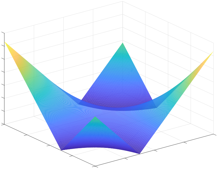
Figure 1: Population objective d1=d2=1.d_{1}=d_{2}=1.

3 Population objective

In this section we study the population objective fPf_{P}. A first important observation is that this function is a singular value function. Indeed, if we set X=w​x⊤−w¯​x¯⊤X=wx^{\top}-\bar{w}\bar{x}^{\top} then due to the orthogonal invariance of the Gaussian distribution we get

fP​(w,x)=𝔼​|a⊤​U​diag​(σ⁡(X))​V⊤​b|=𝔼​|σ1​(X)​a1​b1+σ2​(X)​a2​b2|,f_{P}(w,x)=\mathbb{E}|a^{\top}U{\rm diag}(\sigma(X))V^{\top}b|=\mathbb{E}|\sigma_{1}(X)a_{1}b_{1}+\sigma_{2}(X)a_{2}b_{2}|, (4)

where of course U​diag​(σ⁡(X))​V⊤U{\rm diag}(\sigma(X))V^{\top} is the singular value decomposition of X.X. This simple observation leads to our first result, a closed form characterization of this function in terms σ⁡(X).\sigma(X). We defer the proof to Appendix A.

Proposition 3.1 (Population objective).

The population objective can be written as

fP​(w,x)=σmax​(X)​∑n=0∞((2​n)!22​n​(n!)2)2​(1−κ−2​(X))n1−2​nf_{P}(w,x)=\sigma_{\max}(X)\sum_{n=0}^{\infty}\left(\frac{(2n)!}{2^{2n}(n!)^{2}}\right)^{2}\frac{\left(1-\kappa^{-2}(X)\right)^{n}}{1-2n} (5)

where κ⁡(X)=σmax​(X)/σmin​(X)\kappa(X)={\sigma_{\max}(X)}/{\sigma_{\min}(X)} is the condition number of X.X.

When the signal (w¯,x¯)(\bar{w},\bar{x}) lives in ℝ2\mathbb{R}^{2} the landscape of the population objective is rather simple, the only critical points are the solutions and zero, see Figure 1. This is not the case in higher dimensions where an entire subspace of critical points appear. In the reminder of this section, we develop tools to describe the critical points of a broad class of functions and we then specialize these results to the blind deconvolution population objective (4).

3.1 Landscape analysis for a class of singular value functions

From now on we consider an arbitrary function g:ℝd1×ℝd2→ℝg:\mathbb{R}^{d_{1}}\times\mathbb{R}^{d_{2}}\rightarrow\mathbb{R} for which there exists a rank one matrix w¯​x¯⊤\bar{w}\bar{x}^{\top} and a singular value function fσf_{\sigma} satisfying

g⁡(w,x)=fσ​(w​x⊤−w¯​x¯⊤)=f∘σ⁡(w​x⊤−w¯​x¯⊤).g(w,x)=f_{\sigma}(wx^{\top}-\bar{w}\bar{x}^{\top})=f\circ\sigma\left(wx^{\top}-\bar{w}\bar{x}^{\top}\right).

This gives us two useful characterizations of gg that we will use throughout. In the following section we will see a way of recasting fPf_{P} in this form.

A simple application of the chain rule yields

∂g⁡(w,x)={[Y​xY⊤​w]|Y∈∂fσ​(X)}.\partial g(w,x)=\left\{\begin{bmatrix}Yx\\ Y^{\top}w\end{bmatrix}\,\Big|\,Y\in\partial f_{\sigma}(X)\right\}. (6)

Notice that we already have a description of ∂fσ​(X)\partial f_{\sigma}(X) given by Theorem 2.1, that is Y∈∂fσ​(X)Y\in\partial f_{\sigma}(X) if and only if there exists matrices U∈O⁡(d1)U\in O(d_{1}) and V∈O⁡(d2)V\in O(d_{2}) satisfying

σ(Y)∈∂f(σ(X)),Y=Udiag(σ(Y))V⊤,andX=Udiag(σ(X))V⊤.\sigma(Y)\in\partial f(\sigma(X)),\qquad Y=U{\rm diag}(\sigma(Y))V^{\top},\qquad\text{and}\qquad X=U{\rm diag}(\sigma(X))V^{\top}. (7)

Equipped with these tools we derive the following result regarding the critical points of g.g. We defer a proof to Appendix B.

Theorem 3.1.

Suppose that (w,x)(w,x) is a stationary point for g,g, i.e. Y​x=0,Y⊤​w=0.Yx=0,Y^{\top}w=0. Then at least one of the following conditions hold:

  1. 1.

    Small objective. g⁡(w,x)≤g⁡(w¯,x¯),g(w,x)\leq g(\bar{w},\bar{x}),

  2. 2.

    Zero. (w,x)=0,(w,x)=0,

  3. 3.

    One zero component. ⟨w,w¯⟩=⟨x,x¯⟩=0\langle w,\bar{w}\rangle=\langle x,\bar{x}\rangle=0, w​x⊤=0,wx^{\top}=0, and (assuming that xx is not zero) Y​x=0Yx=0 (similarly for ww).

  4. 4.

    Small product norm. ⟨w,w¯⟩=⟨x,x¯⟩=0\langle w,\bar{w}\rangle=\langle x,\bar{x}\rangle=0, rank⁡(Y)=1\mathrm{rank}(Y)=1, and 0<‖w​x⊤‖<‖w¯​x¯⊤‖.0<\|wx^{\top}\|<\|\bar{w}\bar{x}^{\top}\|.

Moreover, if (w¯,x¯)(\bar{w},\bar{x}) minimizes gg, then (w,x)(w,x) is a critical point if, and only if, it satisfies 1, 2, 3, or 4 for some Y∈∂fσ​(X).Y\in\partial f_{\sigma}(X).

3.2 Landscape of the population objective

Our goal now is to apply Theorem 3.1 to describe the landscape of fP.f_{P}. In order to do it we need to write fP​(w,x)=f∘σ⁡(X)f_{P}(w,x)=f\circ\sigma(X) with f:ℝd→ℝf:\mathbb{R}^{d}\rightarrow\mathbb{R} a symmetric sign-invariant convex function. An easy way to do this is to define

f⁡(s1,…,sd)=𝔼⁡(|∑i=1dai​bi​si|).f(s_{1},\dots,s_{d})=\mathbb{E}\left(\left|\sum_{i=1}^{d}a_{i}b_{i}s_{i}\right|\right).

To use Theorem 3.1, we need to study ∂f.\partial f. The next lemma shows that the function is actually differentiable at every point but zero. We defer the proof of this result to Appendix B.1.

Lemma 3.2.

For any nonzero vector s∈ℝ+d∖{0},s\in\mathbb{R}^{d}_{+}\setminus\{0\}, the partial derivatives of ff satisfy

∂f∂sj​(s)=2π​sj​𝔼​[aj2​(∑id(ai​si)2)−12].\frac{\partial f}{\partial s_{j}}(s)=\sqrt{\frac{2}{\pi}}s_{j}\;\mathbb{E}\left[{a_{j}^{2}}{\left(\sum_{i}^{d}(a_{i}s_{i})^{2}\right)^{-\frac{1}{2}}}\right]. (8)

This lemma gives us the final tool to derive the main theorem regarding the landscape of fP.f_{P}.

Theorem 3.2.

The set of critical points of the population objective gPg_{P} is exactly

𝒮∪{0}∪{(w,x)∣⟨w,w¯⟩=0,⟨x,x¯⟩=0,and wx⊤=0}.\mathcal{S}\cup\{0\}\cup\{(w,x)\mid\langle w,\bar{w}\rangle=0,\langle x,\bar{x}\rangle=0,\text{and }wx^{\top}=0\}.
Proof.

Notice that (w¯,x¯)(\bar{w},\bar{x}) minimizes the population objective fPf_{P}, therefore Theorem 3.1 gives a complete description of the critical points. Let us examine each one of the conditions in this theorem.

The points in {(w,x)∣w​x⊤=w¯​x¯⊤}\{(w,x)\mid wx^{\top}=\bar{w}\bar{x}^{\top}\} and {0}\{0\} are contained in the set of stationary points because they satisfy the first and second condition, respectively.

Now, let (w,x)∈{w¯}⟂×{x¯}⟂(w,x)\in\{\bar{w}\}^{\perp}\times\{\bar{x}\}^{\perp} such that w​x⊤=0.wx^{\top}=0. Thus, the matrix XX is rank 11, and consequently (8) reveals that that any Y∈∂fσ​(X)Y\in\partial f_{\sigma}(X) satisfies σ⁡(Y)=∇f​(σ⁡(X))=(2/π,0,…,0)\sigma(Y)=\nabla f(\sigma(X))=(2/\pi,0,\dots,0). Therefore, due to (7), we get Y=2π​w¯​x¯⊤/‖w¯‖​‖x¯‖.Y=\frac{2}{\pi}\bar{w}\bar{x}^{\top}/\|\bar{w}\|\|\bar{x}\|. Without loss of generality, assume xx is not zero. Then, ‖Y​x‖=2π​‖x¯‖​|⟨x,x¯⟩|=0\left\|Yx\right\|=\frac{2}{\pi\|\bar{x}\|}|\langle x,\bar{x}\rangle|=0 and, consequently, (w,x)(w,x) is stationary.

On the other hand, let (w,x)∈{w¯}⟂×{x¯}⟂(w,x)\in\{\bar{w}\}^{\perp}\times\{\bar{x}\}^{\perp} such that 0<‖w​x⊤‖<‖w¯​x¯⊤‖0<\|wx^{\top}\|<\|\bar{w}\bar{x}^{\top}\|. Therefore, the matrix XX is rank 22 and so (8) gives that σ2​(Y)>0\sigma_{2}(Y)>0 for all Y∈∂fσ​(X).Y\in\partial f_{\sigma}(X). Hence, (w,x)(w,x) is not a stationary point, giving the result. ∎

4 Sample objective

In this section we describe the approximate locations of the critical points of the sample objective. Unlike in the smooth case, nonsmooth losses do not exhibit point-wise concentration of the subgradients, or in other words, ∂fS​(w,x)\partial f_{S}(w,x) doesn’t converges to ∂fP​(w,x)\partial f_{P}(w,x). To overcome this obstacle, we show that the graph of ∂fS\partial f_{S} approaches that of ∂fP\partial f_{P} at a quantifiable rate. This intuitively means that if (w,x)(w,x) is a critical point of fS,f_{S}, then nearby there exists a point (w^,x^)(\widehat{w},\widehat{x}) with dist⁡(0,∂fP​(w^,x^)){\rm dist}(0,\partial f_{P}(\widehat{w},\widehat{x})) small.

The following result can be regarded as an analogous version of Theorem 3.2 for the sample objective. The reasoning behind this theorem is similar: we first develop theory for a broad class of functions, and then specialize it to fS.f_{S}. However, the proof of this result is more involved and will require us to study the location of epsilon critical points of the population. We defer the development of these arguments and the proof of the next result to Appendices C and D, respectively.

Theorem 4.1.

Consider the sample objective (2) generated with two Gaussian matrices AA and BB. For any fixed ν>1\nu>1 there exist numerical constants c1,c2,c3>0c_{1},c_{2},c_{3}>0 such that if m≥c1​(d1+d2+1)m\geq c_{1}(d_{1}+d_{2}+1), then with probability at least 1−c2​exp⁡(−c3​(d1+d2+1))1-c_{2}\exp(-c_{3}(d_{1}+d_{2}+1)), every stationary point (w,x)(w,x) of fSf_{S} for which ‖(w,x)‖≤ν​‖(w¯,x¯)‖\|(w,x)\|\leq\nu\|(\bar{w},\bar{x})\| satisfies at least one of the following conditions

  1. 1.

    Near zero.

    ‖(w,x)‖≤‖(w¯,x¯)‖​Δ,\|(w,x)\|\leq\|(\bar{w},\bar{x})\|\Delta,
  2. 2.

    Near a solution.

    ‖w​x⊤−w¯​x¯⊤‖≲(ν2+1)​‖w¯​x¯⊤‖​Δ,\|wx^{\top}-\bar{w}\bar{x}^{\top}\|\lesssim(\nu^{2}+1)\|\bar{w}\bar{x}^{\top}\|\Delta,
  3. 3.

    Near orthogonal.

    {|⟨w,w¯⟩|≲(ν2+1)​‖(w,x)‖​‖w¯‖​Δ,|⟨x,x¯⟩|≲(ν2+1)​‖(w,x)‖​‖x¯‖​Δ.\left\{\begin{array}[]{rl}|\langle w,\bar{w}\rangle|&\lesssim(\nu^{2}+1)\|(w,x)\|\|\bar{w}\|\Delta,\\ |\langle x,\bar{x}\rangle|&\lesssim(\nu^{2}+1)\|(w,x)\|\|\bar{x}\|\Delta.\end{array}\right.

where Δ=(d1+d2+1m​log⁡(md1+d2+1))18.\Delta=\left(\frac{d_{1}+d_{2}+1}{m}\log\left(\frac{m}{d_{1}+d_{2}+1}\right)\right)^{\frac{1}{8}}.

We remark that one can further prove that with high probability, there exists a neighborhood around the solutions set 𝒮\mathcal{S} in which the only critical points are the solutions [1]. Hence at the cost of potentially increasing c1c_{1}, the second condition can be strengthened to (w¯,x¯)∈𝒮.(\bar{w},\bar{x})\in\mathcal{S}.

5 Experiments

In this section we empirically investigate the behavior of a randomly-initialized subgradient algorithm applied to (2).44 4 The experiments were run in a 2013 MacBook Pro with 2.4 GHz Intel Core i5 Processor and 8 GB of RAM. It is known that well-tuned subgradient algorithms converge to critical points for any locally Lipschitz function [44]. Further, these types of iterative procedures are computationally cheap, easy to implement, and widely used in practice. This makes them a great proxy for our purposes. For the experiments, we use Polyak’s subgradient method, a classical algorithm known to exhibit rapid convergence near solutions for sharp weakly-convex functions [45].55 5 It was shown in [1] that fSf_{S} satisfies these assumptions with high probability provided m≳(d1+d2)m\gtrsim(d_{1}+d_{2}). Polyak’s method is an iterative algorithm given by

xk+1←xk−(f⁡(xk)−inff‖gk‖2)​gkwith ​gk∈∂f⁡(xk).x_{k+1}\leftarrow x_{k}-\left(\frac{f(x_{k})-\inf f}{\|g_{k}\|^{2}}\right)g_{k}\qquad\text{with }g_{k}\in\partial f(x_{k}). (9)

Notice that the step size requires us to know the minimum value, which in this case is exactly zero. Polyak’s algorithm was used in [14] as one of the procedures in the two-stage method for blind deconvolution.

In all the experiments the goal is to recover a pair of canonical vectors (e1,e1)∈ℝd1×ℝd2.(e_{1},e_{1})\in\mathbb{R}^{d_{1}}\times\mathbb{R}^{d_{2}}. Observe that this instance is a good representative of the average performance of the method due to the rotational invariance of the measurements. We evaluate the frequency of successful recovery of (9) using two different random initialization strategies:

  1. 1.

    (Uniform over a cube) We set (w0,x0)(w_{0},x_{0}) to be an uniform vector on the cube [−ν,ν]d1+d2.[-\nu,\nu]^{d_{1}+d_{2}}.

  2. 2.

    (Random Gaussian) We set w0w_{0} and x0x_{0} to be distributed N​(0,ν2d1​Id1)\text{N}(0,\frac{\nu^{2}}{d_{1}}I_{d_{1}}) and N​(0,ν2d2​Id2)\text{N}(0,\frac{\nu^{2}}{d_{2}}I_{d_{2}}), respectively. This ensures that with high probability, both ‖w0‖\|w_{0}\| and ‖x0‖\|x_{0}\| are close to ν.\nu.

We generate phase transition plots for both initialization strategies by varying the value of ν\nu and C≜m/(d1+d2)C\triangleq m/(d_{1}+d_{2}) between {24,25,…,210}\{2^{4},2^{5},\dots,2^{10}\} and {1,2,…,8},\{1,2,\dots,8\}, respectively. For each choice of parameters we generate ten random instances (w0,x0,A,B)(w_{0},x_{0},A,B) and record in how many instances Polyak’s method achieves a relative error smaller than 10−6.10^{-6}. The method stops whenever it reaches 100 000100\,000 iterations or the function value is less than 10−10.10^{-10}. We repeat these experiments for two different pairs of dimensions, (d1,d2)∈{(100,50),(200,100)}(d_{1},d_{2})\in\{(100,50),(200,100)\}. The results are displayed in Figures  and 2.

A first immediate observation is that the random initialization, the dimension, and the scaling parameter ν\nu do not seem to be affecting the recovery frequency of the algorithm. The only parameter that controls the recovery frequency is C.C. This is intuitively consistent with Theorem 4.1, since this parameter determines the concentration of spurious critical points around a subspace. Nonetheless, the effect of this parameter seems to be stronger in practice. Indeed, the probability of recovery exhibits a sharp phase transition at C∼3C\sim 3.

Reproducible research.

All the results and code implemented for these experiments are publicly available in https://github.com/mateodd25/BlindDeconvolutionLandscape.

Figure 2: Empirical probability of recovery with random initialization, first row with Gaussian distribution and second row with uniform over a cube. White denotes probability one and black denotes probability zero. Left and right images correspond to (d1,d2)=(100,50)(d_{1},d_{2})=(100,50) and (d1,d2)=(200,100),(d_{1},d_{2})=(200,100), respectively.

6 Conclusions

We investigated both the population and sample objectives of a formulation for the blind deconvolution problem. We showed that in both cases the set of spurious critical points are, or concentrate near, a subspace of codimension two. Such concentration can be measured in terms of the ratio of the dimension of the signal we wish to recover over the number of measurements. This sheds light on the fact that a randomly-initialized subgradient method converges to a solution whenever this ratio is small enough. Our results, however, do not entirely explain this behavior. It could be the case that we are witnessing an instance of a more general phenomenon. It is known that when the aforementioned ratio is small, the sample objective becomes sharp weakly convex with high probability. It would be interesting to know if for this type of function a well-tuned subgradient method avoids spurious critical points. We leave this as an open question for future research.

Acknowledgments

I thank Jose Bastidas, Damek Davis, Dmitriy Drusvyatskiy, Robert Kleinberg, and Mauricio Velasco for insightful and encouraging conversations. Finally, I would like to thank my advisor Damek Davis for research funding during the completion of this work.

References

  • [1] Vasileios Charisopoulos, Damek Davis, Mateo Díaz, and Dmitriy Drusvyatskiy. Composite optimization for robust blind deconvolution. arXiv preprint arXiv:1901.01624, 2019.
  • [2] E. J. Candès, X. Li, and M. Soltanolkotabi. Phase retrieval via Wirtinger flow: theory and algorithms. IEEE Trans. Inform. Theory, 61(4):1985–2007, 2015.
  • [3] Irène Waldspurger. Phase retrieval with random gaussian sensing vectors by alternating projections. IEEE Transactions on Information Theory, 64(5):3301–3312, 2018.
  • [4] Y. C. Eldar and S. Mendelson. Phase retrieval: stability and recovery guarantees. Appl. Comput. Harmon. Anal., 36(3):473–494, 2014.
  • [5] Xiaodong Li, Shuyang Ling, Thomas Strohmer, and Ke Wei. Rapid, robust, and reliable blind deconvolution via nonconvex optimization. arXiv preprint arXiv:1606.04933, 2016.
  • [6] Dohyung Park, Anastasios Kyrillidis, Constantine Caramanis, and Sujay Sanghavi. Non-square matrix sensing without spurious local minima via the burer-monteiro approach. arXiv preprint arXiv:1609.03240, 2016.
  • [7] Kai Zhong, Prateek Jain, and Inderjit S. Dhillon. Efficient matrix sensing using rank-1 Gaussian measurements. In Algorithmic learning theory, volume 9355 of Lecture Notes in Comput. Sci., pages 3–18. Springer, Cham, 2015.
  • [8] Ruoyu Sun and Zhi-Quan Luo. Guaranteed matrix completion via non-convex factorization. IEEE Trans. Inform. Theory, 62(11):6535–6579, 2016.
  • [9] Rong Ge, Jason D Lee, and Tengyu Ma. Matrix completion has no spurious local minimum. In D. D. Lee, M. Sugiyama, U. V. Luxburg, I. Guyon, and R. Garnett, editors, Advances in Neural Information Processing Systems 29, pages 2973–2981. Curran Associates, Inc., 2016.
  • [10] E. J. Candès, X. Li, Y. Ma, and J. Wright. Robust principal component analysis? J. ACM, 58(3):Art. 11, 37, 2011.
  • [11] Xinyang Yi, Dohyung Park, Yudong Chen, and Constantine Caramanis. Fast algorithms for robust PCA via gradient descent. In Neural Information Processing Systems Conference (NIPS), 2016.
  • [12] Nicolas Boumal, Vlad Voroninski, and Afonso Bandeira. The non-convex burer-monteiro approach works on smooth semidefinite programs. In Advances in Neural Information Processing Systems, pages 2757–2765, 2016.
  • [13] Xiao Li, Zhihui Zhu, Anthony Man-Cho So, and Rene Vidal. Nonconvex robust low-rank matrix recovery. arXiv preprint arXiv:1809.09237, 2018.
  • [14] Vasileios Charisopoulos, Yudong Chen, Damek Davis, Mateo Díaz, Lijun Ding, and Dmitriy Drusvyatskiy. Low-rank matrix recovery with composite optimization: good conditioning and rapid convergence. arXiv preprint arXiv:1904.10020, 2019.
  • [15] Ju sun. Provable nonconvex methods/algorithms. Accessed on 2019-05-13.
  • [16] Yuejie Chi, Yue M Lu, and Yuxin Chen. Nonconvex optimization meets low-rank matrix factorization: An overview. arXiv preprint arXiv:1809.09573, 2018.
  • [17] Rong Ge, Chi Jin, and Yi Zheng. No spurious local minima in nonconvex low rank problems: A unified geometric analysis. arXiv preprint arXiv:1704.00708, 2017.
  • [18] Diego Cifuentes. Burer-monteiro guarantees for general semidefinite programs. arXiv preprint arXiv:1904.07147, 2019.
  • [19] Jason D Lee, Max Simchowitz, Michael I Jordan, and Benjamin Recht. Gradient descent only converges to minimizers. In Conference on learning theory, pages 1246–1257, 2016.
  • [20] Jeongyeol Kwon and Constantine Caramanis. Global convergence of em algorithm for mixtures of two component linear regression. arXiv preprint arXiv:1810.05752, 2018.
  • [21] Lijun Ding and Yudong Chen. The leave-one-out approach for matrix completion: Primal and dual analysis. arXiv preprint arXiv:1803.07554, 2018.
  • [22] Yiqiao Zhong and Nicolas Boumal. Near-optimal bounds for phase synchronization. SIAM Journal on Optimization, 28(2):989–1016, 2018.
  • [23] J. Sun, Q. Qu, and J. Wright. A geometric analysis of phase retrieval. To appear in Found. Comp. Math., arXiv:1602.06664, 2017.
  • [24] Shuyang Ling, Ruitu Xu, and Afonso S Bandeira. On the landscape of synchronization networks: A perspective from nonconvex optimization. arXiv preprint arXiv:1809.11083, 2018.
  • [25] Ali Ahmed, Benjamin Recht, and Justin Romberg. Blind deconvolution using convex programming. IEEE Transactions on Information Theory, 60(3):1711–1732, 2014.
  • [26] Sunav Choudhary and Urbashi Mitra. Sparse blind deconvolution: What cannot be done. In Information Theory (ISIT), 2014 IEEE International Symposium on, pages 3002–3006. IEEE, 2014.
  • [27] Michael Kech and Felix Krahmer. Optimal injectivity conditions for bilinear inverse problems with applications to identifiability of deconvolution problems. SIAM Journal on Applied Algebra and Geometry, 1(1):20–37, 2017.
  • [28] Damek Davis, Dmitriy Drusvyatskiy, and Courtney Paquette. The nonsmooth landscape of phase retrieval. arXiv preprint arXiv:1711.03247, 2017.
  • [29] Ali Ahmed, Alireza Aghasi, and Paul Hand. Blind deconvolutional phase retrieval via convex programming. arXiv preprint arXiv:1806.08091, 2018.
  • [30] Wen Huang and Paul Hand. Blind deconvolution by steepest descent algorithm on a quotient manifold. arXiv preprint arXiv:1710.03309v2, 2018.
  • [31] Cong Ma, Kaizheng Wang, Yuejie Chi, and Yuxin Chen. Implicit regularization in nonconvex statistical estimation: Gradient descent converges linearly for phase retrieval, matrix completion and blind deconvolution. arXiv preprint arXiv:1711.10467, 2017.
  • [32] Yuqian Zhang, Yenson Lau, Han-wen Kuo, Sky Cheung, Abhay Pasupathy, and John Wright. On the global geometry of sphere-constrained sparse blind deconvolution. In Proceedings of the IEEE Conference on Computer Vision and Pattern Recognition, pages 4894–4902, 2017.
  • [33] Han-Wen Kuo, Yenson Lau, Yuqian Zhang, and John Wright. Geometry and symmetry in short-and-sparse deconvolution. arXiv preprint arXiv:1901.00256, 2019.
  • [34] Yanjun Li, Kiryung Lee, and Yoram Bresler. Identifiability in blind deconvolution with subspace or sparsity constraints. IEEE Transactions on Information Theory, 62(7):4266–4275, 2016.
  • [35] Cedric Josz, Yi Ouyang, Richard Zhang, Javad Lavaei, and Somayeh Sojoudi. A theory on the absence of spurious optimality. arXiv preprint arXiv:1805.08204, 2018.
  • [36] Salar Fattahi and Somayeh Sojoudi. Exact guarantees on the absence of spurious local minima for non-negative robust principal component analysis. arXiv preprint arXiv:1812.11466, 2018.
  • [37] Yu Bai, Qijia Jiang, and Ju Sun. Subgradient descent learns orthogonal dictionaries. arXiv preprint arXiv:1810.10702, 2018.
  • [38] R. T. Rockafellar and R. J-B. Wets. Variational Analysis. Grundlehren der mathematischen Wissenschaften, Vol 317, Springer, Berlin, 1998.
  • [39] B. S. Mordukhovich. Variational analysis and generalized differentiation. I, volume 330 of Grundlehren der Mathematischen Wissenschaften [Fundamental Principles of Mathematical Sciences]. Springer-Verlag, Berlin, 2006. Basic theory.
  • [40] J. M. Borwein and Q. J. Zhu. Techniques of Variational Analysis. Springer Verlag, New York, 2005.
  • [41] A. S. Lewis. Derivatives of spectral functions. Math. Oper. Res., 21(3):576–588, 1996.
  • [42] A. S. Lewis. Nonsmooth analysis of eigenvalues. Math. Program., 84(1, Ser. A):1–24, 1999.
  • [43] Adrian S Lewis and Hristo S Sendov. Nonsmooth analysis of singular values. part i: Theory. Set-Valued Analysis, 13(3):213–241, 2005.
  • [44] Damek Davis, Dmitriy Drusvyatskiy, Sham Kakade, and Jason D. Lee. Stochastic subgradient method converges on tame functions. Foundations of Computational Mathematics, Jan 2019.
  • [45] Damek Davis, Dmitriy Drusvyatskiy, Kellie J. MacPhee, and Courtney Paquette. Subgradient methods for sharp weakly convex functions. arXiv preprint arXiv:1803.02461, 2018.
  • [46] Inder K. Rana. An introduction to measure and integration, volume 45 of Graduate Studies in Mathematics. American Mathematical Society, Providence, RI, second edition, 2002.

Appendix A Proof of Proposition 3.1

Recall that we defined the functions f:ℝ+d→ℝf:\mathbb{R}^{d}_{+}\rightarrow\mathbb{R} and fσ:ℝd×n→ℝf_{\sigma}:\mathbb{R}^{d\times n}\rightarrow\mathbb{R} to be such that fP​(w,x)=fσ​(X)=f⁡(σ⁡(X)).f_{P}(w,x)=f_{\sigma}(X)=f(\sigma(X)). It is known that for constants c1,c2∈ℝ+c_{1},c_{2}\in\mathbb{R}_{+} we have that c1​b1+c2​b2=(d)c12+c22​b1,c_{1}b_{1}+c_{2}b_{2}\stackrel{{\scriptstyle(d)}}{{=}}\sqrt{c_{1}^{2}+c_{2}^{2}}b_{1}, where =(d)\stackrel{{\scriptstyle(d)}}{{=}} denotes equality in distribution. Then

f⁡(s1,s2,0,…,0)\displaystyle f(s_{1},s_{2},0,\dots,0) =𝔼⁡(|s1​a1​b1+s2​a2​b2|)\displaystyle=\mathbb{E}(|s_{1}a_{1}b_{1}+s_{2}a_{2}b_{2}|)
=𝔼⁡(𝔼⁡(|s1​a1​b1+s2​a2​b2|∣a1,a2))\displaystyle=\mathbb{E}\left(\mathbb{E}(|s_{1}a_{1}b_{1}+s_{2}a_{2}b_{2}|\mid a_{1},a_{2})\right)
=𝔼⁡(𝔼⁡((s1​a1)2+(s2​a2)2​|b1|∣a1,a2))\displaystyle=\mathbb{E}\left(\mathbb{E}(\sqrt{(s_{1}a_{1})^{2}+(s_{2}a_{2})^{2}}|b_{1}|\mid a_{1},a_{2})\right)
=2π​𝔼​(s1​a1)2+(s2​a2)2\displaystyle=\sqrt{\frac{2}{\pi}}\mathbb{E}\sqrt{(s_{1}a_{1})^{2}+(s_{2}a_{2})^{2}}
=π2​π2​∫−∞∞∫−∞∞(a1​s1)2+(a2​s2)2​exp⁡(−a12+a222)​d​a1​d​a2\displaystyle=\frac{\sqrt{\pi}}{\sqrt{2}\pi^{2}}\int_{-\infty}^{\infty}\int_{-\infty}^{\infty}{\sqrt{(a_{1}s_{1})^{2}+(a_{2}s_{2})^{2}}}\exp\left(-\frac{a_{1}^{2}+a_{2}^{2}}{2}\right)da_{1}da_{2}
=4​π2​π2​∫0∞∫0∞(a1​s1)2+(a2​s2)2​exp⁡(−a12+a222)​d​a1​d​a2\displaystyle=4\frac{\sqrt{\pi}}{\sqrt{2}\pi^{2}}\int_{0}^{\infty}\int_{0}^{\infty}{\sqrt{(a_{1}s_{1})^{2}+(a_{2}s_{2})^{2}}}\exp\left(-\frac{a_{1}^{2}+a_{2}^{2}}{2}\right)da_{1}da_{2}
=2​2​ππ2​∫0∞∫0π/2r2​s12​cos2⁡θ+s22​sin2⁡θ​exp⁡(−r22)​𝑑θ​𝑑r\displaystyle=2\frac{\sqrt{2\pi}}{\pi^{2}}\int_{0}^{\infty}\int_{0}^{\pi/2}r^{2}{\sqrt{s_{1}^{2}\cos^{2}\theta+s_{2}^{2}\sin^{2}\theta}}\exp\left(-\frac{r^{2}}{2}\right)d\theta dr
=2π​∫0π/2s12​cos2⁡θ+s22​sin2⁡θ​𝑑θ\displaystyle=\frac{2}{\pi}\int_{0}^{\pi/2}{\sqrt{s_{1}^{2}\cos^{2}\theta+s_{2}^{2}\sin^{2}\theta}}d\theta
=2​s1π​∫0π/2cos2⁡θ+s22s12​sin2⁡θ​𝑑θ\displaystyle=\frac{2s_{1}}{\pi}\int_{0}^{\pi/2}{\sqrt{\cos^{2}\theta+\frac{s_{2}^{2}}{s_{1}^{2}}\sin^{2}\theta}}d\theta
=2​s1π​∫0π/21−(1−s22s12)​sin2⁡θ​𝑑θ\displaystyle=\frac{2s_{1}}{\pi}\int_{0}^{\pi/2}{\sqrt{1-\left(1-\frac{s_{2}^{2}}{s_{1}^{2}}\right)\sin^{2}\theta}}d\theta
=2​s1π​E​(1−s22s12)\displaystyle=\frac{2s_{1}}{\pi}E\left(1-\frac{s_{2}^{2}}{s_{1}^{2}}\right)

where E⁡(⋅)E(\cdot) is the complete elliptic integral of the second kind (with parameter m=k2m=k^{2}). Thus altogether we obtain

fσ​(X)=σmax​(X)​∑n=0∞((2​n)!22​n​(n!)2)2​(1−κ−2​(X))n1−2​nf_{\sigma}(X)=\sigma_{\max}(X)\sum_{n=0}^{\infty}\left(\frac{(2n)!}{2^{2n}(n!)^{2}}\right)^{2}\frac{\left(1-\kappa^{-2}(X)\right)^{n}}{1-2n}

where κ⁡(X)=σmax​(X)/σmin​(X)\kappa(X)={\sigma_{\max}(X)}/{\sigma_{\min}(X)} is the condition number of X.X.

Appendix B Proof of Theorem 3.1

The proof of this result builds upon the next three lemmas. We will prove these lemmas and before we dive into the proof. Recall that U∈O⁡(d1)U\in O(d_{1}) and V∈O⁡(d2)V\in O(d_{2}) are any pair of matrices for which X=U​σ​(X)​V=∑iσi​(X)​Ui​Vi⊤.X=U\sigma(X)V=\sum_{i}\sigma_{i}(X)U_{i}V_{i}^{\top}.

Lemma B.1.

The following are true.

  1. 1.

    Anticorrelation. The next equalities hold

    ⟨U1,w⟩​⟨x,V2⟩=⟨U1,w¯⟩​⟨x¯,V2⟩and⟨U2,w⟩​⟨x,V1⟩=⟨U2,w¯⟩​⟨x¯,V1⟩.\langle U_{1},w\rangle\langle x,V_{2}\rangle=\langle U_{1},\bar{w}\rangle\langle\bar{x},V_{2}\rangle\qquad\text{and}\qquad\langle U_{2},w\rangle\langle x,V_{1}\rangle=\langle U_{2},\bar{w}\rangle\langle\bar{x},V_{1}\rangle.
  2. 2.

    Singular values. The singular values of XX satisfy

    σ1​(X)=⟨U1,w⟩​⟨x,V1⟩−⟨U1,w¯⟩​⟨x¯,V1⟩≥0,σ2​(X)=⟨U2,w⟩​⟨x,V2⟩−⟨U2,w¯⟩​⟨x¯,V2⟩≥0.\begin{array}[]{c}\sigma_{1}(X)=\langle U_{1},w\rangle\langle x,V_{1}\rangle-\langle U_{1},\bar{w}\rangle\langle\bar{x},V_{1}\rangle\geq 0,\\ \sigma_{2}(X)=\langle U_{2},w\rangle\langle x,V_{2}\rangle-\langle U_{2},\bar{w}\rangle\langle\bar{x},V_{2}\rangle\geq 0.\end{array}
  3. 3.

    Correlation. Assume that σ2​(w​x⊤−w¯​x¯⊤)>0,\sigma_{2}(wx^{\top}-\bar{w}\bar{x}^{\top})>0, then span​{x,x¯}=span​{V1,V2}\text{span}\{x,\bar{x}\}=\text{span}\{V_{1},V_{2}\}, span​{w,w¯}=span​{U1,U2}\text{span}\{w,\bar{w}\}=\text{span}\{U_{1},U_{2}\}, and consequently,

    ⟨w,w¯⟩\displaystyle\langle w,\bar{w}\rangle =⟨U1,w⟩​⟨U1,w¯⟩+⟨U2,w⟩​⟨U2,w¯⟩,\displaystyle=\langle U_{1},w\rangle\langle U_{1},\bar{w}\rangle+\langle U_{2},w\rangle\langle U_{2},\bar{w}\rangle,
    ⟨x,x¯⟩\displaystyle\langle x,\bar{x}\rangle =⟨V1,x⟩​⟨V1,x¯⟩+⟨V2,x⟩​⟨V2,x¯⟩.\displaystyle=\langle V_{1},x\rangle\langle V_{1},\bar{x}\rangle+\langle V_{2},x\rangle\langle V_{2},\bar{x}\rangle.
Proof.

The first equality in item one follows by observing that U1⊤​X​V2=0U_{1}^{\top}XV_{2}=0, expanding the expression on the left-hand-side gives the result. The same argument starting from U2⊤​X​V1=0U_{2}^{\top}XV_{1}=0 gives the other equality. The second item follows by definition.

To prove the last item note that

⟨Ui,w⟩​x−⟨Ui,w¯⟩​x¯=X⊤​Ui=σi​(X)​Vi∀i∈{1,2}.\langle U_{i},w\rangle x-\langle U_{i},\bar{w}\rangle\bar{x}=X^{\top}U_{i}=\sigma_{i}(X)V_{i}\qquad\forall i\in\{1,2\}.

Dividing through by σi​(X)\sigma_{i}(X) in the previous inequality shows that span​{x,x¯}=span​{V1,V2}\text{span}\{x,\bar{x}\}=\text{span}\{V_{1},V_{2}\}. Therefore, we can write x=⟨x,V1⟩​V1+⟨x,V2⟩​V2x=\langle x,V_{1}\rangle V_{1}+\langle x,V_{2}\rangle V_{2} and x¯=⟨x¯,V1⟩​V1+⟨x¯,V2⟩​V2.\bar{x}=\langle\bar{x},V_{1}\rangle V_{1}+\langle\bar{x},V_{2}\rangle V_{2}. Hence,

⟨x,x¯⟩=⟨⟨x,V1⟩​V1+⟨x,V2⟩​V2,⟨x¯,V1⟩​V1+⟨x¯,V2⟩​V2⟩=⟨V1,x⟩​⟨V1,x¯⟩+⟨V2,x⟩​⟨V2,x¯⟩\langle x,\bar{x}\rangle=\left\langle\langle x,V_{1}\rangle V_{1}+\langle x,V_{2}\rangle V_{2},\langle\bar{x},V_{1}\rangle V_{1}+\langle\bar{x},V_{2}\rangle V_{2}\right\rangle=\langle V_{1},x\rangle\langle V_{1},\bar{x}\rangle+\langle V_{2},x\rangle\langle V_{2},\bar{x}\rangle

An analogous argument shows the statement for ww and w¯\bar{w}. ∎

Lemma B.2.

The following hold true.

  1. 1.

    Maximum correlation.

    max⁡{|σ1​(Y)​⟨v1,x⟩|,|σ2​(Y)​⟨v2,x⟩|}≤‖Y​x‖,max⁡{|σ1​(Y)​⟨u1,w⟩|,|σ2​(Y)​⟨u2,w⟩|}≤‖Y⊤​w‖.\begin{array}[]{c}\max\{|\sigma_{1}(Y)\langle v_{1},x\rangle|,|\sigma_{2}(Y)\langle v_{2},x\rangle|\}\leq\|Yx\|,\\ \max\{|\sigma_{1}(Y)\langle u_{1},w\rangle|,|\sigma_{2}(Y)\langle u_{2},w\rangle|\}\leq\|Y^{\top}w\|.\end{array} (10)
  2. 2.

    Objective gap.

    g⁡(w,x)−g⁡(w¯,x¯)≤σ1​(Y)​σ1​(X)+σ2​(Y)​σ2​(X).g(w,x)-g(\bar{w},\bar{x})\leq\sigma_{1}(Y)\sigma_{1}(X)+\sigma_{2}(Y)\sigma_{2}(X). (11)
Proof.

Note that ‖Y​x‖≥⟨z,Y​x⟩\|Yx\|\geq\langle z,Yx\rangle for all z∈𝕊d−1z\in{\mathbb{S}}^{d-1}, then the very first claim follows by testing with z∈{±U1,±U2}.z\in\{\pm U_{1},\pm U_{2}\}. An analogous argument gives the statement for w.w. Recall that ff is convex, consequently fσf_{\sigma} is convex and the subgradient inequality gives

g⁡(w,x)−g⁡(w¯,x¯)=fσ​(X)−fσ​(0)≤⟨Y,X⟩=σ1​(Y)​σ1​(X)+σ2​(Y)​σ1​(X).g(w,x)-g(\bar{w},\bar{x})=f_{\sigma}(X)-f_{\sigma}(0)\leq\langle Y,X\rangle=\sigma_{1}(Y)\sigma_{1}(X)+\sigma_{2}(Y)\sigma_{1}(X).

∎

Lemma B.3.

Assume w¯∈ℝd1\bar{w}\in\mathbb{R}^{d_{1}} and x¯∈ℝd2\bar{x}\in\mathbb{R}^{d_{2}} are nonzero vectors. Set X=w​x⊤+w¯​x¯⊤X=wx^{\top}+\bar{w}\bar{x}^{\top}, then XX is a rank 11 matrix if, and only if, w=λ​w¯w=\lambda\bar{w} or x=λ​x¯x=\lambda\bar{x} for some λ∈ℝ.\lambda\in\mathbb{R}.

Proof.

It is trivial to see that if the later holds then XX is rank 1.1. Let us prove the other direction. Notice that if any of the vectors is zero we are done, so assume that none of them is. Recall that all the columns of XX are span from one vector. Consider the case where xx and x¯\bar{x} have different support (i.e. set of nonzero entries), then it is immediate that ww and w¯\bar{w} have to be multiples of each other.

Now assume that this is not the case, without loss of generality assume that w∉span​{w¯}w\notin\text{span}\{\bar{w}\} and xx and x¯\bar{x} are nonzero and their first component is equal to one. Then the first column of XX is equal to w+w¯w+\bar{w}, furthermore the second column is equal to x2​w+x¯2​w¯x_{2}w+\bar{x}_{2}\bar{w} has to be a multiple of the first one. By assumption w,w¯w,\bar{w} are linearly independent therefore x2=x¯2.x_{2}=\bar{x}_{2}. Using the same procedure for the rest of the entries we obtain x=x¯.x=\bar{x}. ∎

We are now in good shape to describe the landscape of the function g.g.

Proof of Theorem 3.1.

To prove that at least one of the conditions hold we will show that if the first two don’t hold then at least one of the other two have two hold. Assume that that the first two conditions are not satisfied, therefore g⁡(w,x)>g⁡(w¯,x¯)g(w,x)>g(\bar{w},\bar{x}) and (w,x)≠(0,0).(w,x)\neq(0,0). Let us furnished some facts before we prove this is the case. Notice that from (11) we can derive

0<σ1​(Y)​σ1​(X)+σ2​(Y)​σ1​(X)≤2​σ1​(Y)​σ1​(X),0<\sigma_{1}(Y)\sigma_{1}(X)+\sigma_{2}(Y)\sigma_{1}(X)\leq 2\sigma_{1}(Y{})\sigma_{1}(X),

thus σ1​(Y),σ1​(X)>0.\sigma_{1}(Y),\sigma_{1}(X)>0. On the other hand, since (w,x)(w,x) is critical inequalities (10) immediately give

σ1​(Y)​⟨V1,x⟩=σ2​(Y)​⟨V2,x⟩=0,andσ1​(Y)​⟨U1,w⟩=σ2​(Y)​⟨U2,w⟩=0.\displaystyle\begin{split}&\sigma_{1}(Y)\langle V_{1},x\rangle=\sigma_{2}(Y)\langle V_{2},x\rangle=0,\qquad\text{and}\qquad\sigma_{1}(Y)\langle U_{1},w\rangle=\sigma_{2}(Y)\langle U_{2},w\rangle=0.\end{split} (12)

So ⟨V1,x⟩=0\langle V_{1},x\rangle=0 and ⟨U1,w⟩=0\langle U_{1},w\rangle=0, then the first claim in Lemma B.1 gives. Additionally, this and the second claim in Lemma B.1 imply that

⟨U1,w¯⟩​⟨x¯,V2⟩=⟨U2,w¯⟩​⟨x¯,V1⟩=0,and−⟨U1,w¯⟩​⟨x¯,V1⟩=σ1​(X)>0.\displaystyle\langle U_{1},\bar{w}\rangle\langle\bar{x},V_{2}\rangle=\langle U_{2},\bar{w}\rangle\langle\bar{x},V_{1}\rangle=0,\qquad\text{and}\qquad-\langle U_{1},\bar{w}\rangle\langle\bar{x},V_{1}\rangle=\sigma_{1}(X)>0.

Combining these two gives ⟨U2,w¯⟩=⟨x¯,V2⟩=0.\langle U_{2},\bar{w}\rangle=\langle\bar{x},V_{2}\rangle=0. Then by applying the second claim in Lemma B.1 we get σ2​(X)=⟨U2,w⟩​⟨x,V2⟩\sigma_{2}(X)=\langle U_{2},w\rangle\langle x,V_{2}\rangle. Using Equations (12) we conclude that σ2​(Y)​σ2​(X)=0.\sigma_{2}(Y)\sigma_{2}(X)=0.

Now we will show that at least one of the conditions holds, depending on the value of σ2​(X),\sigma_{2}(X), let us consider two cases:

Case 1. Assume σ2​(X)=0.\sigma_{2}(X)=0. This means that X=w​x⊤−w¯​x¯⊤X=wx^{\top}-\bar{w}\bar{x}^{\top} is a rank 11 matrix. By Lemma B.3 we have that w=λ​w¯w=\lambda\bar{w} or x=λ​x¯x=\lambda\bar{x} for some λ∈ℝ.\lambda\in\mathbb{R}. Note that if w=λ​w¯w=\lambda\bar{w} then U1=±w¯/∥w¯∥U_{1}=\pm\bar{w}/\|\bar{w}\|, then using Equation 12 we get that λ​‖w¯‖=0.\lambda\|\bar{w}\|=0. Which implies that λ=0,\lambda=0, and consequently w​x⊤=0.wx^{\top}=0. An analogous argument applies when x=λ​x¯.x=\lambda\bar{x}. By assumption we have that Y​x=0Yx=0 and Y⊤​w=0Y^{\top}w=0. Additionally, since X=−w¯​x¯⊤X=-\bar{w}\bar{x}^{\top} we get that that U1=±w¯/∥w¯∥U_{1}=\pm\bar{w}/\|\bar{w}\| and V1=±x¯/∥x¯∥.V_{1}=\pm\bar{x}/\|\bar{x}\|. Recall that Y=U​diag​(σ⁡(Y))​V⊤,Y=U{\rm diag}(\sigma(Y))V^{\top}, then using the fact that (w,x)(w,x) is critical we conclude ⟨w,w¯⟩=⟨x,x¯⟩=0.\langle w,\bar{w}\rangle=\langle x,\bar{x}\rangle=0. Implying that property three holds.

Case 2. Assume σ2​(X)≠0.\sigma_{2}(X)\neq 0. This immediately implies that σ2​(Y)=0.\sigma_{2}(Y)=0. By the third part of Lemma B.1 we get that

⟨x,x¯⟩=⟨V1,x⟩​⟨V1,x¯⟩+⟨V2,x⟩​⟨V2,x¯⟩=0\langle x,\bar{x}\rangle=\langle V_{1},x\rangle\langle V_{1},\bar{x}\rangle+\langle V_{2},x\rangle\langle V_{2},\bar{x}\rangle=0

and analogously ⟨w,w¯⟩=0.\langle w,\bar{w}\rangle=0. Moreover, since w⟂w¯w\perp\bar{w} and x⟂w¯x\perp\bar{w} (and none of them are zero by assumption) we get that (w/‖w‖,x/‖x‖)(w/\|w\|,x/\|x\|) and (w¯/‖w¯‖,x¯/‖x¯‖)(\bar{w}/\|\bar{w}\|,\bar{x}/\|\bar{x}\|) are pairs of left and right singular vectors, with associated singular values w⊤​X​x=‖w​x⊤‖w^{\top}Xx=\|wx^{\top}\| and w¯⊤​X​x¯=‖w¯​x¯⊤‖\bar{w}^{\top}X\bar{x}=\|\bar{w}\bar{x}^{\top}\|, respectively. Assume that ‖w​x⊤‖≥‖w¯​x¯⊤‖,\|wx^{\top}\|\geq\|\bar{w}\bar{x}^{\top}\|, thus 0=w⊤​Y​x=‖w​x⊤‖​σ1​(Y)>0,0=w^{\top}Yx=\|wx^{\top}\|\sigma_{1}(Y)>0, yielding a contradiction. Hence the condition four holds true.

Finally, we will prove the reverse statement. Assume that (w¯,x¯)(\bar{w},\bar{x}) minimize g.g. In this case, the set of points that satisfies the first conditions is the collection of minimizers so they are critical. Clearly (w,x)=0(w,x)=0 is always a stationary point, since ‖Y⊤​w‖=‖Y​x‖=0\|Y^{\top}w\|=\|Yx\|=0. Now let’s construct a certificate Y∈∂fσ​(X)Y\in\partial f_{\sigma}(X) that ensures criticality for the remaining cases.

Assume that (w,x)(w,x) that w​x⊤=0,wx^{\top}=0, without loss of generality let’s assume that w=0.w=0. Further, assume that there exists Y∈∂fσ​(w,x)Y\in\partial f_{\sigma}(w,x) such that Y​x=0Yx=0 and ⟨x,x¯⟩=0.\langle x,\bar{x}\rangle=0. It is immediate that (w,x)(w,x) is a stationary point.

Assume that (w,x)(w,x) is such that 0<‖w​x⊤‖<‖w¯​x¯⊤‖,0<\|wx^{\top}\|<\|\bar{w}\bar{x}^{\top}\|, ⟨w,w¯⟩=⟨x,x¯⟩=0\langle w,\bar{w}\rangle=\langle x,\bar{x}\rangle=0 and there exists Y∈∂fσ​(X)Y\in\partial f_{\sigma}(X) with σ2​(Y)=0.\sigma_{2}(Y)=0. By our argument above since ‖w​x⊤‖<‖w¯​x¯⊤‖\|wx^{\top}\|<\|\bar{w}\bar{x}^{\top}\|, any pair of admissible matrices U,VU,V satisfy U1=±w¯/∥w¯∥U_{1}=\pm\bar{w}/\|\bar{w}\| and V1=±x¯/∥x¯∥.V_{1}=\pm\bar{x}/\|\bar{x}\|. Therefore

Y​x=(σ1​(Y)​U1​V1⊤)​x=±σ1​(Y)‖x¯‖​⟨x¯,x⟩​U1=0,Yx=(\sigma_{1}(Y)U_{1}V_{1}^{\top})x=\pm\frac{\sigma_{1}(Y)}{\|\bar{x}\|}\langle\bar{x},x\rangle U_{1}=0,

analogously Y⊤​w=0.Y^{\top}w=0. ∎

B.1 Proof of Lemma 3.2

It is well-known that if (a1,a2,…,ad)(a_{1},a_{2},\dots,a_{d}) is fixed (i.e. if we conditioned on it), then

∑i=1dai​bi​si=(d)(∑i=1d(ai​si)2)12​b\sum_{i=1}^{d}a_{i}b_{i}s_{i}\stackrel{{\scriptstyle(d)}}{{=}}\left(\sum_{i=1}^{d}(a_{i}s_{i})^{2}\right)^{\frac{1}{2}}b

and bb is a standard normal random variable independent of the rest of the data. Therefore

f⁡(s1,…,sd)\displaystyle f(s_{1},\dots,s_{d}) =𝔼⁡(|∑i=1dai​bi​si|)=𝔼⁡(𝔼⁡(|∑i=1dai​bi​si||a1,…,ad))\displaystyle=\mathbb{E}\left(\left|\sum_{i=1}^{d}a_{i}b_{i}s_{i}\right|\right)=\mathbb{E}\left(\mathbb{E}\left(\left|\sum_{i=1}^{d}a_{i}b_{i}s_{i}\right|\Big|a_{1},\dots,a_{d}\right)\right)
=𝔼⁡((∑i=1d(ai​si)2)12​𝔼​(b∣a1,…,ad))=2π​𝔼​(∑i=1d(ai​si)2)12.\displaystyle=\mathbb{E}\left(\left(\sum_{i=1}^{d}(a_{i}s_{i})^{2}\right)^{\frac{1}{2}}\mathbb{E}\left(b\mid a_{1},\dots,a_{d}\right)\right)=\sqrt{\frac{2}{\pi}}\mathbb{E}\left(\sum_{i=1}^{d}(a_{i}s_{i})^{2}\right)^{\frac{1}{2}}.

Now, we need a technical tool in order to procede.

Theorem B.1 (Leibniz Integral Rule, Theorem 5.4.12 in [46]).

Let UU be an open subset of ℝd\mathbb{R}^{d} and Ω\Omega be a measure space. Suppose that the function h:U×Ω→ℝh:U\times\Omega\rightarrow\mathbb{R} satisfies the following:

  1. 1.

    For all x∈Ux\in U, the function h⁡(x,⋅)h(x,\cdot) is Lebesgue integrable.

  2. 2.

    For almost all w∈Ωw\in\Omega, if we define hω​(⋅)=f⁡(⋅,ω)h^{\omega}(\cdot)=f(\cdot,\omega) the partial derivatives ∂hω∂xi​(x)\frac{\partial h^{\omega}}{\partial x_{i}}(x) exists for all x∈Ux\in U.

  3. 3.

    There is an integrable function Φ:Ω→ℝ\Phi:\Omega\rightarrow\mathbb{R} such that |∂hω∂xi​(x)|≤Φ​(ω)|\frac{\partial h^{\omega}}{\partial x_{i}}(x)|\leq\Phi(\omega) for all x∈Ux\in U and almost every ω∈Ω.\omega\in\Omega.

Then, we have that for all x∈Ux\in U

∂∂xi​∫Ωh⁡(x,ω)​𝑑ω=∫Ω∂hω∂xi​(x)​𝑑ω.\frac{\partial}{\partial x_{i}}\int_{\Omega}h(x,\omega)d\omega=\int_{\Omega}\frac{\partial h^{\omega}}{\partial x_{i}}(x)d\omega.

This theorem tell us that we can swap partial derivatives and integrals provided that the function satisfies all the conditions above. Consider Ω\Omega to be the set ℝd\mathbb{R}^{d} endow with the Borel σ\sigma-algebra and the multivariate Gaussian measure. Define h:ℝd×Ω→ℝh:\mathbb{R}^{d}\times\Omega\rightarrow\mathbb{R} to be given by

(s,a)↦(∑i=1d(ai​si)2)12.(s,a)\mapsto\left(\sum_{i=1}^{d}(a_{i}s_{i})^{2}\right)^{\frac{1}{2}}.

Take s∈ℝd∖{0}s\in\mathbb{R}^{d}\setminus\{0\} to be an arbitary element, set S={u∈ℝd∣supp⁡(s)⊆supp⁡(u)}S=\{u\in\mathbb{R}^{d}\mid{\mathrm{supp}}(s)\subseteq{\mathrm{supp}}(u)\}, and define U=Bϵ​(s)U=B_{\epsilon}(s) with ϵ\epsilon small enough such that U⊆SU\subseteq S and infu∈Umini∈supp⁡(s)⁡|ui|>0\inf_{u\in U}\min_{i\in{\mathrm{supp}}(s)}|u_{i}|>0. Then it is easy to see that the first two conditions hold, in particular the second condition hold for all a≠0a\neq 0. Further, for any x∈Ux\in U

|∂ha∂sj​(x)|=|aj2​xj(∑id(ai​xi)2)12|\displaystyle\left|\frac{\partial h^{a}}{\partial s_{j}}(x)\right|=\left|\frac{a_{j}^{2}x_{j}}{\left(\sum_{i}^{d}(a_{i}x_{i})^{2}\right)^{\frac{1}{2}}}\right| ≤supu∈U‖u‖∞infu∈Umini∈supp⁡(s)⁡|ui|​∑i∈supp⁡(s)aj2(∑i∈supp⁡(s)ai2)12\displaystyle\leq\frac{\sup_{u\in U}\|u\|_{\infty}}{\inf_{u\in U}\min_{i\in{\mathrm{supp}}(s)}|u_{i}|}\frac{\sum_{i\in{\mathrm{supp}}(s)}a_{j}^{2}}{\left(\sum_{i\in{\mathrm{supp}}(s)}a_{i}^{2}\right)^{\frac{1}{2}}}
≤supu∈U‖u‖∞infu∈Umini⁡|ui|​(∑i∈supp⁡(s)ai2)12,\displaystyle\leq\frac{\sup_{u\in U}\|u\|_{\infty}}{\inf_{u\in U}\min_{i}|u_{i}|}{\left(\sum_{i\in{\mathrm{supp}}(s)}a_{i}^{2}\right)^{\frac{1}{2}}},

where the last function is integrable with respect to the Gaussian measure. Thus, Theorem B.1 ensures that the function ff is differentiable at every nonzero point. Consequently, for all s∈ℝd∖{0}s\in\mathbb{R}^{d}\setminus\{0\}

∂f∂sj​(s)=2π​sj​𝔼​aj2(∑id(ai​si)2)12.\frac{\partial f}{\partial s_{j}}(s)=\sqrt{\frac{2}{\pi}}s_{j}\;\mathbb{E}\frac{a_{j}^{2}}{\left(\sum_{i}^{d}(a_{i}s_{i})^{2}\right)^{\frac{1}{2}}}.

Appendix C Approximate critical points of a spectral function family

In Section 3 we characterize the points for which 0∈∂fP​(w,x).0\in\partial f_{P}(w,x). In order to derive similar results for fSf_{S} we will need to understand ε\varepsilon-critical points of fP,f_{P}, i.e. points (w,x)(w,x) for which dist⁡(0,∂f⁡(w,x))≤ε.{\rm dist}(0,\partial f(w,x))\leq\varepsilon. Just as before we adopt a more general viewpoint and consider spectral functions of the form g⁡(w,x)=f∘σ⁡(w​x⊤−w¯​x¯⊤).g(w,x)=f\circ\sigma(wx^{\top}-\bar{w}\bar{x}^{\top}).

The main result in this section is Theorem C.1. Given the fact that we don’t have second order information in the form of a Hessian, we need to appeal to a different kind of growth condition. Turns out that the natural condition for this problem is

g⁡(w,x)−g⁡(w¯,x¯)≥κ​‖w​x⊤−w¯​x¯⊤‖F∀(w,x)∈ℝd1×ℝd2,g(w,x)-g(\bar{w},\bar{x})\geq\kappa\left\|wx^{\top}-\bar{w}\bar{x}^{\top}\right\|_{F}\qquad\forall(w,x)\in\mathbb{R}^{d_{1}}\times\mathbb{R}^{d_{2}}, (13)

for some κ>0.\kappa>0. Intuitively this means that the function grows sharply away from minimizers.

Before we dive into the main theorem, let us provide some technical lemmas.

Lemma C.1.

Suppose there exists a constant κ>0\kappa>0 such that (13) holds. Then, for any point (w,x)(w,x) such that w​x⊤≠w¯​x¯⊤wx^{\top}\neq\bar{w}\bar{x}^{\top} we have σ1​(Y)+σ2​(Y)≥κ.\sigma_{1}(Y)+\sigma_{2}(Y)\geq\kappa.

Proof.

By definition σ2​(X)≤σ1​(X)≤‖w​x⊤−w¯​x¯⊤‖F\sigma_{2}(X)\leq\sigma_{1}(X)\leq\left\|wx^{\top}-\bar{w}\bar{x}^{\top}\right\|_{F}. Then, applying (11) gives

κ​‖w​x⊤−w¯​x¯⊤‖F≤g⁡(w,x)−g⁡(w¯,x¯)\displaystyle\kappa\left\|wx^{\top}-\bar{w}\bar{x}^{\top}\right\|_{F}\leq g(w,x)-g(\bar{w},\bar{x}) ≤σ1​(Y)​σ1​(X)+σ2​(Y)​σ2​(X)\displaystyle\leq\sigma_{1}(Y)\sigma_{1}(X)+\sigma_{2}(Y)\sigma_{2}(X)
≤(σ1​(Y)+σ2​(Y))​‖w​x⊤−w¯​x¯⊤‖F.\displaystyle\leq(\sigma_{1}(Y)+\sigma_{2}(Y))\left\|wx^{\top}-\bar{w}\bar{x}^{\top}\right\|_{F}.

∎

Lemma C.2.

Suppose there exists a constant κ>0\kappa>0 such that (13) holds. Then any pair (w,x)∈ℝd1+d2∖{0}(w,x)\in\mathbb{R}^{d_{1}+d_{2}}\setminus\{0\} satisfies

1min⁡{‖w‖,‖x‖}​(κ⁡‖w​x⊤−w¯​x¯⊤‖−(σ1​(Y)+σ2​(Y))​‖w¯​x¯⊤‖)≤dist⁡(0,∂g⁡(w,x)).\frac{1}{{\min\{\left\|w\right\|,\left\|x\right\|\}}}\left(\kappa\left\|wx^{\top}-\bar{w}\bar{x}^{\top}\right\|-(\sigma_{1}(Y)+\sigma_{2}(Y))\left\|\bar{w}\bar{x}^{\top}\right\|\right)\leq{\rm dist}(0;\partial g(w,x)).
Proof.

Notice that the result holds trivially for any pair such that w​x⊤=w¯​x¯⊤.wx^{\top}=\bar{w}\bar{x}^{\top}. Let’s assume that this is not the case. Recall that ∂g⁡(w,x)=∂fσ​(X)​x×(∂fσ​(X))⊤​w.\partial g(w,x)=\partial f_{\sigma}(X)x\times(\partial f_{\sigma}(X))^{\top}w. Pick Y∈∂g⁡(w,x)Y\in\partial g(w,x) such that dist⁡(0,∂g⁡(w,x))=‖Y​x‖2+‖Y⊤​w‖2.{\rm dist}(0,\partial g(w,x))=\sqrt{\|Yx\|^{2}+\|Y^{\top}w\|^{2}}. Using the convexity of fσf_{\sigma} we get

κ​‖w​x⊤−w¯​x¯‖F≤g⁡(w,x)−g⁡(w¯,x¯)\displaystyle\kappa\|wx^{\top}-\bar{w}\bar{x}\|_{F}\leq g(w,x)-g(\bar{w},\bar{x}) =fσ​(X)−fσ​(0)\displaystyle=f_{\sigma}(X)-f_{\sigma}(0)
≤⟨Y,w​x⊤−w¯​x¯⊤⟩\displaystyle\leq\langle Y,wx^{\top}-\bar{w}\bar{x}^{\top}\rangle
≤‖x‖​‖Y⊤​w‖+|w⊤​Y​x|≤‖x‖​dist​(0,∂g⁡(w,x))+|w⊤​Y​x|,\displaystyle\leq\|x\|\|Y^{\top}w\|+|w^{\top}Yx|\leq\|x\|{\rm dist}(0,\partial g(w,x))+|w^{\top}Yx|,

where the last inequality follows by Cauchy-Schwartz. Applying the same argument using w⊤​Y​x≤‖w‖​‖Y​x‖w^{\top}Yx\leq\|w\|\|Yx\| gives

g⁡(w,x)−g⁡(w¯,x¯)≤min⁡{‖w‖,‖x‖}​dist​(0,∂g⁡(w,x))+|w⊤​Y​x|.g(w,x)-g(\bar{w},\bar{x})\leq\min\{\|w\|,\|x\|\}{\rm dist}(0,\partial g(w,x))+|w^{\top}Yx|.

Now, let’s bound the second term on the right-hand-side. Note that

|w¯⊤​Y​x¯|=|⟨Y,w​x⊤⟩|≤‖Y‖​‖w​x⊤‖≤(σ1​(Y)+σ2​(Y))​‖w¯​x¯⊤‖.|\bar{w}^{\top}Y\bar{x}|=|\langle Y,wx^{\top}\rangle|\leq\|Y\|\|wx^{\top}\|\leq(\sigma_{1}(Y)+\sigma_{2}(Y))\left\|\bar{w}\bar{x}^{\top}\right\|.

The result follows immediately. ∎

We can now prove the main result of this section, a detailed location description of ε\varepsilon-critical points. This can be thought of as a quantitative version of Corollary 3.1. Its proof is however more involved due to the inexactness of the assumptions.

Theorem C.1.

Assume that ‖w¯‖=‖x¯‖\|\bar{w}\|=\|\bar{x}\| and that there exists a constant κ>0\kappa>0 such that (13) holds. Further assume that σ1​(Y)\sigma_{1}(Y) is bounded by some numerical constant.66 6 This is implied for example when ff is Lipschitz. Let ζ=(Y​x,Y⊤​w)∈∂g⁡(w,x)\zeta=(Yx,Y^{\top}w)\in\partial g(w,x), and set ε=‖ζ‖.\varepsilon=\|\zeta\|. Then if w​x⊤=0wx^{\top}=0 we have that

max⁡{‖Y​x‖,‖Y⊤​w‖}≤ε,and{|⟨w,w¯⟩|≲ε​‖w¯‖|⟨x,x¯⟩|≲ε​‖x¯‖.\max\{\|Yx\|,\|Y^{\top}w\|\}\leq\varepsilon,\qquad\text{and}\qquad\left\{\begin{array}[]{ll}|\langle w,\bar{w}\rangle|&\lesssim\varepsilon\|\bar{w}\|\\ |\langle x,\bar{x}\rangle|&\lesssim\varepsilon\|\bar{x}\|\end{array}\right..

On the other hand, if w​x⊤≠0wx^{\top}\neq 0 and ‖(w,x)‖≤ν​‖(w¯,x¯)‖\|(w,x)\|\leq\nu\|(\bar{w},\bar{x})\| for some fixed ν>1\nu>1. There exists a constant77 7 Independent of ν\nu. γ>0\gamma>0 such that if ε≤γ​max⁡{‖w‖,‖x‖}\varepsilon\leq\gamma\max\{\|w\|,\|x\|\} then ‖w​x⊤‖≲‖w¯​x¯⊤‖\left\|wx^{\top}\right\|\lesssim\left\|\bar{w}\bar{x}^{\top}\right\| and at least one of the following holds

  1. 1.
    max⁡{‖w‖,‖x‖}​‖w​x⊤−w¯​x¯⊤‖≲ε⁡‖w¯​x¯⊤‖\max\{\left\|w\right\|,\left\|x\right\|\}\left\|wx^{\top}-\bar{w}\bar{x}^{\top}\right\|\lesssim\varepsilon\left\|\bar{w}\bar{x}^{\top}\right\|
  2. 2.
    min⁡{‖w‖,‖x‖}≲εand{|⟨w,w¯⟩|≲ν2​ε​‖w¯‖|⟨x,x¯⟩|≲ν2​ε​‖x¯‖.\min\{\|w\|,\|x\|\}\lesssim\varepsilon\qquad\text{and}\qquad\left\{\begin{array}[]{ll}|\langle w,\bar{w}\rangle|&\lesssim\nu^{2}\varepsilon\|\bar{w}\|\\ |\langle x,\bar{x}\rangle|&\lesssim\nu^{2}\varepsilon\|\bar{x}\|\end{array}\right..
  3. 3.
    σ2​(Y)≲εmax⁡{‖w‖,‖x‖} and {|⟨w,w¯⟩|≲ν2​ε​‖w¯‖|⟨x,x¯⟩|≲ν2​ε​‖x¯‖.\sigma_{2}(Y)\lesssim\frac{\varepsilon}{\max\{\|w\|,\|x\|\}}\qquad\text{ and }\qquad\left\{\begin{array}[]{ll}|\langle w,\bar{w}\rangle|&\lesssim\nu^{2}\varepsilon\|\bar{w}\|\\ |\langle x,\bar{x}\rangle|&\lesssim\nu^{2}\varepsilon\|\bar{x}\|\end{array}\right..
Proof.

First assume that w​x⊤=0,wx^{\top}=0, then it is clear that max⁡{‖Y​x‖,‖Y⊤​w‖}=‖ζ‖≤ε\max\{\|Yx\|,\|Y^{\top}w\|\}=\|\zeta\|\leq\varepsilon. Without loss of generality assume that x=0,x=0, let Y=U​σ​(Y)​V⊤Y=U\sigma(Y)V^{\top} be the singular value decomposition. Since X=−w¯​x¯⊤X=-\bar{w}\bar{x}^{\top} then U1=±w¯/∥w¯∥U_{1}=\pm\bar{w}/\|\bar{w}\| and V1=±x¯/‖x¯‖V_{1}=\pm\bar{x}/\left\|\bar{x}\right\| and so

ε≥‖Y⊤​w‖=‖σ1​(Y)‖w¯‖​⟨w¯,w⟩​V1+z‖≥σ1​(Y)‖w¯‖​|⟨w¯,w⟩|≥κ2​‖w¯‖​⟨w¯,w⟩\varepsilon\geq\|Y^{\top}w\|=\left\|\frac{\sigma_{1}(Y)}{\|\bar{w}\|}\langle{\bar{w}},w\rangle V_{1}+z\right\|\geq\frac{\sigma_{1}(Y)}{\|\bar{w}\|}\left|\langle{\bar{w}},w\rangle\right|\geq\frac{\kappa}{2\left\|\bar{w}\right\|}\langle{\bar{w}},w\rangle (14)

where zz is orthogonal to V1V_{1} and the second inequality follows by Lemma C.1. This proves the first statement in the theorem.

We know move to the “On the other hand” statement, assume w​x⊤≠0wx^{\top}\neq 0 and ‖(w,x)‖≤ν​‖(w¯,x¯)‖\|(w,x)\|\leq\nu\|(\bar{w},\bar{x})\|. Notice that the result holds immediately if (w,x)∈{(α​w¯,x¯/α)∣α∈ℝ}(w,x)\in\{(\alpha\bar{w},\bar{x}/\alpha)\mid\alpha\in\mathbb{R}\}. Further, due to Theorem 3.1 it also holds when ε=0\varepsilon=0. Let us assume that none of these two conditions are satisfied.

We will start by showing that ‖w​x⊤‖≲‖w¯​x¯⊤‖.\left\|wx^{\top}\right\|\lesssim\left\|\bar{w}\bar{x}^{\top}\right\|. Set

δ=2κ​(σ1​(Y)+σ2​(Y))+1.\delta=\frac{\sqrt{2}}{\kappa}(\sigma_{1}(Y)+\sigma_{2}(Y))+1. (15)

We showed in Lemma C.1 that (σ1​(Y)+σ2​(Y))≥κ(\sigma_{1}(Y)+\sigma_{2}(Y))\geq\kappa and thus δ>1.\delta>1.

Claim 1.

The inequality ‖w​x⊤‖≤δ⁡‖w¯​x¯⊤‖\left\|wx^{\top}\right\|\leq\delta\left\|\bar{w}\bar{x}^{\top}\right\| holds true.

Proof.

Seeking contradiction assume that this is not the case. By the previous lemma

2‖w​x⊤‖​κ​‖w​x⊤−w¯​x¯⊤‖−εmax⁡{‖w‖,‖x‖}≤(σ1​(Y)+σ2​(Y))​‖w¯​x¯⊤‖‖w​x⊤‖.\frac{\sqrt{2}}{{\left\|wx^{\top}\right\|}}\kappa\left\|wx^{\top}-\bar{w}\bar{x}^{\top}\right\|-\frac{\varepsilon}{\max\{\|w\|,\|x\|\}}\leq(\sigma_{1}(Y)+\sigma_{2}(Y))\frac{\left\|\bar{w}\bar{x}^{\top}\right\|}{\left\|wx^{\top}\right\|}. (16)

Notice that

2‖w​x⊤‖​κ​‖w​x⊤−w¯​x¯⊤‖=2​κ​‖w​x⊤‖w​x⊤‖−w¯​x¯⊤‖w​x⊤‖‖≥2​κ​|1−1δ|.\frac{\sqrt{2}}{{\left\|wx^{\top}\right\|}}\kappa\left\|wx^{\top}-\bar{w}\bar{x}^{\top}\right\|={\sqrt{2}}\kappa\left\|\frac{wx^{\top}}{{\left\|wx^{\top}\right\|}}-\frac{\bar{w}\bar{x}^{\top}}{{{\left\|wx^{\top}\right\|}}}\right\|\geq\sqrt{2}\kappa\left|1-\frac{1}{\delta}\right|.

If we set γ<2​κ2​|1−1δ|\gamma<\frac{\sqrt{2}\kappa}{2}\left|1-\frac{1}{\delta}\right| then we ensure εmax⁡{‖w‖,‖x‖}<2​κ2​|1−1δ|,\frac{\varepsilon}{\max\{\|w\|,\|x\|\}}<\frac{\sqrt{2}\kappa}{2}\left|1-\frac{1}{\delta}\right|, thus

2​κ​|1−1δ|2​(σ1​(Y)+σ2​(Y))\displaystyle\frac{\sqrt{2}\kappa\left|1-\frac{1}{\delta}\right|}{2(\sigma_{1}(Y)+\sigma_{2}(Y))} ≤1(σ1​(Y)+σ2​(Y))​(2‖w​x⊤‖​κ​‖w​x⊤−w¯​x¯⊤‖−εmax⁡{‖w‖,‖x‖})\displaystyle\leq\frac{1}{(\sigma_{1}(Y)+\sigma_{2}(Y))}\left(\frac{\sqrt{2}}{{\left\|wx^{\top}\right\|}}\kappa\left\|wx^{\top}-\bar{w}\bar{x}^{\top}\right\|-\frac{\varepsilon}{\max\{\|w\|,\|x\|\}}\right)
≤‖w¯​x¯⊤‖‖w​x⊤‖<1δ.\displaystyle\leq\frac{\left\|\bar{w}\bar{x}^{\top}\right\|}{\left\|wx^{\top}\right\|}<\frac{1}{\delta}.

Rearranging we get

|δ−1|<2κ​(σ1​(Y)+σ2​(Y)),|\delta-1|<\frac{\sqrt{2}}{\kappa}(\sigma_{1}(Y)+\sigma_{2}(Y)),

leading to a contradiction. ∎

We now move on to proving that at least one of the three conditions has to hold. To this end, define

ρ1=max⁡{‖w‖,‖x‖}2andρ2=1κ​max⁡{2​2​(1+δ),4​σ1​(Y)}​‖w¯​x¯⊤‖max⁡{‖w‖,‖x‖}.\rho_{1}=\frac{\max\{\|w\|,\|x\|\}}{\sqrt{2}}\qquad\text{and}\qquad\rho_{2}=\frac{1}{\kappa}\max\big\{2\sqrt{2}(1+\delta),4\sigma_{1}(Y)\big\}\frac{\left\|\bar{w}\bar{x}^{\top}\right\|}{\max\{\|w\|,\|x\|\}}.

Observe that if assume that if ε​ρ2≥‖w​x⊤−w¯​x¯⊤‖\varepsilon\rho_{2}\geq\left\|wx^{\top}-\bar{w}\bar{x}^{\top}\right\| then the result holds immediately. Assume from now on that ε​ρ2<‖w​x⊤−w¯​x¯⊤‖.\varepsilon\rho_{2}<\left\|wx^{\top}-\bar{w}\bar{x}^{\top}\right\|. Our road map is as follows, we will start by assuming min⁡{‖w‖,‖x‖}≤2​ε/κ\min\{\|w\|,\|x\|\}\leq 2\varepsilon/\kappa and we will show that this implies the second condition in item two. Then we will move to assume that min⁡{‖w‖,‖x‖}>2​ε/κ\min\{\|w\|,\|x\|\}>2\varepsilon/\kappa and show that item three has to hold.

Before we continue let us list some important facts. By Lemma B.2

max⁡{σ1​(Y)​|⟨V1,x⟩|,σ2​(Y)​|⟨V2,x⟩|,σ1​(Y)​|⟨U1,w⟩|,σ2​(Y)​|⟨U2,w⟩|}≤ε\max\{\sigma_{1}(Y)|\langle V_{1},x\rangle|,\sigma_{2}(Y)|\langle V_{2},x\rangle|,\sigma_{1}(Y)|\langle U_{1},w\rangle|,\sigma_{2}(Y)|\langle U_{2},w\rangle|\}\leq\varepsilon (17)

which together with σ1​(Y)>κ/2\sigma_{1}(Y)>\kappa/2 implies that

max⁡{|⟨U1,w⟩|,|⟨V1,x⟩|}≤εσ1​(Y)≤2​εκ.\max\{\left|\langle U_{1},w\rangle\right|,\left|\langle V_{1},x\rangle\right|\}\leq\frac{\varepsilon}{\sigma_{1}(Y)}\leq\frac{2\varepsilon}{\kappa}. (18)

Notice that this implies by Lemma B.1

|⟨U1,w¯⟩​⟨x¯,V2⟩|=|⟨U1,w⟩​⟨x,V2⟩|≤2​‖x‖​εκand|⟨U2,w¯⟩​⟨x¯,V1⟩|≤2​‖w‖​εκ.|\langle U_{1},\bar{w}\rangle\langle\bar{x},V_{2}\rangle|=|\langle U_{1},w\rangle\langle x,V_{2}\rangle|\leq\frac{2\|x\|\varepsilon}{\kappa}\qquad\text{and}\qquad\left|\langle U_{2},\bar{w}\rangle\langle\bar{x},V_{1}\rangle\right|\leq\frac{2\|w\|\varepsilon}{\kappa}. (19)

Observe that

max⁡{‖w‖,‖x‖}≤‖(w,x)‖≤ν|(w¯,x¯)|=2​ν​min​{‖w¯‖,‖x¯‖}.\max\{\|w\|,\|x\|\}\leq\|(w,x)\|\leq\nu\|(\bar{w},\bar{x})\|=\sqrt{2}\nu\min\{\|\bar{w}\|,\|\bar{x}\|\}. (20)

We can now continue with the proof. We will now assume that min⁡{‖w‖,‖x‖}≤4​δ​ε/κ\min\{\|w\|,\|x\|\}\leq 4\delta\varepsilon/\kappa and prove that item two holds.

Claim 2.

Assume that min⁡{‖w‖,‖x‖}≤4​δ​ε/κ.\min\{\|w\|,\|x\|\}\leq 4\delta\varepsilon/\kappa. Then

|⟨w,w¯⟩|≲ν2​ε​‖w¯‖ and |⟨x,x¯⟩|≲ν2​ε​‖x¯‖.|\langle w,\bar{w}\rangle|\lesssim\nu^{2}\varepsilon\|\bar{w}\|\qquad\text{ and }\qquad|\langle x,\bar{x}\rangle|\lesssim\nu^{2}\varepsilon\|\bar{x}\|.
Proof.

Notice

|⟨w,w¯‖w¯‖⟩|≤|⟨w,w¯‖w¯‖−U1⟩|+|⟨w,U1⟩|≤‖w‖​‖w¯‖w¯‖−U1‖+2​εκ\displaystyle\left|\langle w,\frac{\bar{w}}{\|\bar{w}\|}\rangle\right|\leq\left|\langle w,\frac{\bar{w}}{\|\bar{w}\|}-U_{1}\rangle\right|+\left|\langle w,U_{1}\rangle\right|\leq\|w\|\left\|\frac{\bar{w}}{\|\bar{w}\|}-U_{1}\right\|+\frac{2\varepsilon}{\kappa}

where the last inequality follows by Cauchy-Schwartz and (18). A similar argument gives the same bound with ‖w¯/‖w¯‖+U1‖\left\|\bar{w}/\|\bar{w}\|+U_{1}\right\| instead. Now we need to make use of the Davis-Kahan Theorem.

Theorem C.2.

Let A,A^∈ℝd1×d2A,\widehat{A}\in\mathbb{R}^{d_{1}\times d_{2}} with rank⁡(A)=1.\mathrm{rank}(A)=1. Let A=U​σ​(A)​V⊤A=U\sigma(A)V^{\top} and A^=U^​σ​(A^)​V^⊤\widehat{A}=\widehat{U}\sigma(\widehat{A})\widehat{V}^{\top} be their singular value decompositions. Then the

sin⁡θ⁡(V1,V^1)≤2​(2​σ1​(A)+‖A−A^‖op)‖A‖2​‖A−A^‖,\sin\theta(V_{1},\widehat{V}_{1})\leq\frac{2(2\sigma_{1}(A)+\|A-\widehat{A}\|_{\mathrm{op}})}{\|A\|^{2}}\|A-\widehat{A}\|,

the same bound holds for U1,U^1.U_{1},\widehat{U}_{1}.

By letting A=−w¯​x¯⊤A=-\bar{w}\bar{x}^{\top} and A^=w​x⊤−w¯​x¯⊤\widehat{A}=wx^{\top}-\bar{w}\bar{x}^{\top} in the previous theorem we get

min⁡{‖w¯‖w¯‖+U1‖,‖w¯‖w¯‖−U1‖}\displaystyle\min\left\{\left\|\frac{\bar{w}}{\|\bar{w}\|}+U_{1}\right\|,\left\|\frac{\bar{w}}{\|\bar{w}\|}-U_{1}\right\|\right\} ≤2​sin⁡(θ⁡(w¯/‖w¯‖,U1))\displaystyle\leq\sqrt{2}\sin\left(\theta(\bar{w}/\|\bar{w}\|,U_{1})\right)
≤2​2​(2​‖w¯​x¯⊤‖+‖w​x⊤‖)‖w¯​x¯⊤‖2​‖w​x⊤‖\displaystyle\leq 2\sqrt{2}\frac{(2\|\bar{w}\bar{x}^{\top}\|+\|wx^{\top}\|)}{\|\bar{w}\bar{x}^{\top}\|^{2}}\|wx^{\top}\|
≤2​2​(2+δ)​‖w​x⊤‖‖w¯​x¯⊤‖\displaystyle\leq 2\sqrt{2}(2+\delta)\frac{\|wx^{\top}\|}{\|\bar{w}\bar{x}^{\top}\|}
≤2​2​(2+δ)​ν​ε‖w¯‖\displaystyle\leq 2\sqrt{2}(2+\delta)\nu\frac{\varepsilon}{\|\bar{w}\|}

where the last inequality follows since ‖w​x⊤‖≤ε​max⁡{‖w‖,‖x‖}\|wx^{\top}\|\leq\varepsilon\max\{\|w\|,\|x\|\} and (20). Hence from the previous inequalities we derive

|⟨w,w¯‖w¯‖⟩|≤‖w‖​‖w¯‖w¯‖−U1‖+2​εκ≤2​2​(2+δ)​ν​‖w‖‖w¯‖​ε+2​εκ=(2​2​(2+δ)​ν2+2κ)​ε.\left|\langle w,\frac{\bar{w}}{\|\bar{w}\|}\rangle\right|\leq\|w\|\left\|\frac{\bar{w}}{\|\bar{w}\|}-U_{1}\right\|+\frac{2\varepsilon}{\kappa}\leq 2\sqrt{2}(2+\delta)\nu\frac{\|w\|}{\|\bar{w}\|}\varepsilon+\frac{2\varepsilon}{\kappa}=\left(2\sqrt{2}(2+\delta)\nu^{2}+\frac{2}{\kappa}\right)\varepsilon.

A completely analogous result holds for |⟨x,x¯⟩|.|\langle x,\bar{x}\rangle|. ∎

Suppose now that min⁡{‖w‖,‖x‖}>4​δ​ε/κ.\min\{\|w\|,\|x\|\}>4\delta\varepsilon/\kappa. In the remainder of the proof we will show that in this case, item three has to hold.

Claim 3.

The rank of X=w​x⊤−w¯​x¯⊤X=wx^{\top}-\bar{w}\bar{x}^{\top} is two.

Proof.

Assume w=λ​w¯w=\lambda\bar{w}, then U1=±w/∥w¯∥U_{1}=\pm w/\|\bar{w}\| and using the same computation as in Equation (14) we get λ​‖w¯‖≤2​ϵ/κ≤4​δ​ϵ/κ\lambda\|\bar{w}\|\leq 2\epsilon/\kappa\leq 4\delta\epsilon/\kappa which implies min⁡{‖w‖,‖x‖}≤4​δ​ε/κ,\min\{\|w\|,\|x\|\}\leq 4\delta\varepsilon/\kappa, yielding a contradiction. An analogous argument holds for x=λ​x¯.x=\lambda\bar{x}. Thus, Lemma B.3 implies that σ2​(w​x⊤−w¯​x¯⊤)>0.\sigma_{2}(wx^{\top}-\bar{w}\bar{x}^{\top})>0. ∎

Claim 4.

σ2​(Y)<ερ1.\sigma_{2}(Y)<\frac{\varepsilon}{\rho_{1}}.

Proof.

Without loss of generality suppose ‖w‖=max⁡{‖w‖,‖x‖}.\|w\|=\max\{\|w\|,\|x\|\}. Assume seeking contradiction that this isn’t true, thus σ2​(Y)≥ε/ρ1\sigma_{2}(Y)\geq\varepsilon/\rho_{1} then Inequality (17) gives |⟨U2,w⟩|≤ρ1.|\langle U_{2},w\rangle|\leq\rho_{1}. Furthermore, notice that due to Lemma B.1 we have that ‖w‖2=⟨U1,w⟩2+⟨U2,w⟩2\|w\|^{2}=\langle U_{1},w\rangle^{2}+\langle U_{2},w\rangle^{2} and consequently |⟨U1,w⟩|≥‖w‖2−ρ12.|\langle U_{1},w\rangle|\geq\sqrt{\|w\|^{2}-\rho_{1}^{2}}. Again, due to (17)

σ1​(Y)≤ε|⟨U1,w⟩|≤ε‖w‖2−ρ12.\sigma_{1}(Y)\leq\frac{\varepsilon}{|\langle U_{1},w\rangle|}\leq\frac{\varepsilon}{\sqrt{\|w\|^{2}-\rho_{1}^{2}}}.

In turn this implies

κ​ε​ρ2<κ⁡‖w​x⊤−w¯​x¯⊤‖≤g⁡(w,x)−g⁡(w¯,x¯)\displaystyle\kappa\varepsilon\rho_{2}<\kappa\left\|wx^{\top}-\bar{w}\bar{x}^{\top}\right\|\leq g(w,x)-g(\bar{w},\bar{x}) ≤σ1​(Y)​σ1​(X)+σ2​(Y)​σ2​(X)\displaystyle\leq\sigma_{1}(Y)\sigma_{1}(X)+\sigma_{2}(Y)\sigma_{2}(X)
≤2​σ1​(Y)​σ1​(X)\displaystyle\leq 2\sigma_{1}(Y)\sigma_{1}(X)
≤2​ε‖w‖2−ρ12​|⟨U1,w⟩​⟨x,V1⟩−⟨U1,w¯⟩​⟨x¯,V1⟩|\displaystyle\leq 2\frac{\varepsilon}{\sqrt{\|w\|^{2}-\rho_{1}^{2}}}|\langle U_{1},w\rangle\langle x,V_{1}\rangle-\langle U_{1},\bar{w}\rangle\langle\bar{x},V_{1}\rangle|
≤2​ε‖w‖2−ρ12​(‖w​x⊤‖+‖w¯​x¯⊤‖)\displaystyle\leq 2\frac{\varepsilon}{\sqrt{\|w\|^{2}-\rho_{1}^{2}}}\left(\left\|wx^{\top}\right\|+\left\|\bar{w}\bar{x}^{\top}\right\|\right)
≤2​2​ε‖w‖​(1+δ)​‖w¯​x¯⊤‖\displaystyle\leq\frac{2\sqrt{2}\varepsilon}{\|w\|}\left(1+\delta\right)\left\|\bar{w}\bar{x}^{\top}\right\|

Rearranging we get

ρ<2​2​(1+δ)κ​‖w¯​x¯⊤‖max⁡{‖w‖,‖x‖},\rho<\frac{2\sqrt{2}(1+\delta)}{\kappa}\frac{\left\|\bar{w}\bar{x}^{\top}\right\|}{\max\{\|w\|,\|x\|\}},

yielding a contradiction. ∎

We now need to prove an additional claim.

Claim 5.

|⟨U2,w¯⟩|≤|⟨U1,w¯⟩|\left|\langle U_{2},\bar{w}\rangle\right|\leq\left|\langle U_{1},\bar{w}\rangle\right| and |⟨V2,x¯⟩|≤|⟨V1,x¯⟩|\left|\langle V_{2},\bar{x}\rangle\right|\leq\left|\langle V_{1},\bar{x}\rangle\right|

Proof.

Seeking contradiction we assume the possible contrary cases.

Case 1. Assume |⟨U2,w¯⟩|>|⟨U1,w¯⟩|\left|\langle U_{2},\bar{w}\rangle\right|>\left|\langle U_{1},\bar{w}\rangle\right| and |⟨V2,x¯⟩|>|⟨U1,x¯⟩|\left|\langle V_{2},\bar{x}\rangle\right|>\left|\langle U_{1},\bar{x}\rangle\right|, then(18) and (19) imply

max⁡{|⟨U1,w⟩​⟨V1,x⟩|,|⟨U1,w¯⟩​⟨V1,x¯⟩|}≤2​min⁡{‖w‖,‖x‖}​εκ.\max\{|\langle U_{1},w\rangle\langle V_{1},x\rangle|,|\langle U_{1},\bar{w}\rangle\langle V_{1},\bar{x}\rangle|\}\leq\frac{2\min\{\|w\|,\|x\|\}\varepsilon}{\kappa}.

From which we derive

κ​ε​ρ2<g⁡(w,x)−g⁡(w¯,x¯)≤2​σ1​(Y)​σ1​(X)≤4​σ1​(Y)​δ​‖w¯​x¯⊤‖max⁡{‖w‖,‖x‖}​ε.\displaystyle\kappa\varepsilon\rho_{2}<g(w,x)-g(\bar{w},\bar{x})\leq 2\sigma_{1}(Y)\sigma_{1}(X)\leq 4\sigma_{1}(Y)\delta\frac{\left\|\bar{w}\bar{x}^{\top}\right\|}{\max\{\|w\|,\|x\|\}}\varepsilon.

contradicting the definition of ρ2.\rho_{2}.

Case 2. Assume that |⟨U2,w¯⟩|≤|⟨U1,w¯⟩|\left|\langle U_{2},\bar{w}\rangle\right|\leq\left|\langle U_{1},\bar{w}\rangle\right| and |⟨V2,x¯⟩|>|⟨V1,x¯⟩|.\left|\langle V_{2},\bar{x}\rangle\right|>\left|\langle V_{1},\bar{x}\rangle\right|. Notice that ‖w¯‖2=⟨U1,w¯⟩2+⟨U2,w¯⟩2\|\bar{w}\|^{2}=\langle U_{1},\bar{w}\rangle^{2}+\langle U_{2},\bar{w}\rangle^{2}, hence |⟨U1,w¯⟩|≥‖w¯‖/2\left|\langle U_{1},\bar{w}\rangle\right|\geq\|\bar{w}\|/\sqrt{2} and similarly |⟨V2,x¯⟩|>‖x¯‖/2.\left|\langle V_{2},\bar{x}\rangle\right|>\|\bar{x}\|/\sqrt{2}. Thus,

‖w¯‖2≤|⟨U1,w¯⟩|≤2​‖x‖​εκ​|⟨x¯,V2⟩|<2​2|x|εκ​‖x¯‖.\frac{\|\bar{w}\|}{\sqrt{2}}\leq|\langle U_{1},\bar{w}\rangle|\leq\frac{2\|x\|\varepsilon}{\kappa|\langle\bar{x},V_{2}\rangle|}<\frac{2\sqrt{2}\|x\|\varepsilon}{\kappa\|\bar{x}\|}.

This implies that

min⁡{‖w‖,‖x‖}≤‖w‖≤δ​‖w¯​x¯⊤‖‖x‖<4​δ​εκ,\min\{\|w\|,\|x\|\}\leq\|w\|\leq\delta\frac{\left\|\bar{w}\bar{x}^{\top}\right\|}{\|x\|}<\frac{4\delta\varepsilon}{\kappa},

yielding a contradiction. ∎

Without loss of generality let us assume ‖w‖≤‖x‖.\|w\|\leq\|x\|.

Claim 6.
|⟨w,w¯⟩|≲ε⁡‖w¯‖and|⟨x,x¯⟩|≲ν2​ε​‖x¯‖.\left|\langle w,\bar{w}\rangle\right|\lesssim\varepsilon\left\|\bar{w}\right\|\qquad\text{and}\qquad\left|\langle x,\bar{x}\rangle\right|\lesssim\nu^{2}\varepsilon\left\|\bar{x}\right\|.
Proof.

By the previous claim and the fact that ‖w¯‖2=⟨U1,w¯⟩2+⟨U2,w¯⟩2\|\bar{w}\|^{2}=\langle U_{1},\bar{w}\rangle^{2}+\langle U_{2},\bar{w}\rangle^{2} we get that |⟨U1,w¯⟩|≥‖w‖/2|\langle U_{1},\bar{w}\rangle|\geq\|w\|/\sqrt{2}, combining this with (19) gives

|⟨x¯,V2⟩|≤2​2|x|εκ​‖w¯‖≤4​δκ​ν​ε|\langle\bar{x},V_{2}\rangle|\leq\frac{2\sqrt{2}\|x\|\varepsilon}{\kappa\|\bar{w}\|}\leq\frac{4\delta}{\kappa}\nu\varepsilon

Then by Lemma B.1

|⟨x,x¯⟩|=|⟨V1,x⟩​⟨V1,x¯⟩+⟨V2,x⟩​⟨V2,x¯⟩|\displaystyle\left|\langle x,\bar{x}\rangle\right|=|\langle V_{1},x\rangle\langle V_{1},\bar{x}\rangle+\langle V_{2},x\rangle\langle V_{2},\bar{x}\rangle| ≤|⟨V1,x⟩​⟨V1,x¯⟩|+|⟨V2,x⟩​⟨V2,x¯⟩|\displaystyle\leq|\langle V_{1},x\rangle\langle V_{1},\bar{x}\rangle|+|\langle V_{2},x\rangle\langle V_{2},\bar{x}\rangle|
≤2​εκ​‖x¯‖+‖x‖​|⟨V2,x¯⟩|\displaystyle\leq\frac{2\varepsilon}{\kappa}\|\bar{x}\|+\|x\||\langle V_{2},\bar{x}\rangle|
≤(2κ+4​δκ​ν2)​ε​‖x¯‖≤(2κ+4​δκ​ν2)​ε​‖x¯‖.\displaystyle\leq\left(\frac{2}{\kappa}+\frac{4\delta}{\kappa}\nu^{2}\right)\varepsilon\|\bar{x}\|\leq\left(\frac{2}{\kappa}+\frac{4\delta}{\kappa}\nu^{2}\right)\varepsilon\|\bar{x}\|.

where we used (20). Notice that the same analysis gives

|⟨w,w¯⟩|≤(2κ+2​2​δκ​‖w‖‖x‖)​ε​‖w¯‖≤(2κ+2​2​δκ)​ε​‖w¯‖.\left|\langle w,\bar{w}\rangle\right|\leq\left(\frac{2}{\kappa}+\frac{2\sqrt{2}\delta}{\kappa}\frac{\|w\|}{\|x\|}\right)\varepsilon\|\bar{w}\|\leq\left(\frac{2}{\kappa}+\frac{2\sqrt{2}\delta}{\kappa}\right)\varepsilon\|\bar{w}\|.

∎

This last claim finishes the proof of the theorem. ∎

Appendix D Proofs of Theorem 4.1

In order to prove the theorem we will apply three steps: we will show that the graphs of ∂fS\partial f_{S} and ∂fP\partial f_{P} are close, then use Theorem C.1 to study the ϵ\epsilon-critical points of fPf_{P} and finally conclude about the landscape of fSf_{S} by combining the previous two steps. The following two propositions handle the first part.

Proposition D.1.

Fix two functions f,g:ℝd1×ℝd2→ℝf,g:\mathbb{R}^{d_{1}}\times\mathbb{R}^{d_{2}}\rightarrow\mathbb{R} such that gg is ρ\rho-weakly convex. Suppose that there exists a point (w¯,x¯)(\bar{w},\bar{x}) and a real δ>0\delta>0 such that the inequality

|f⁡(w,x)−g⁡(w,x)|≤δ​‖w​x⊤−w¯​x¯⊤‖Fholds for all ​(w,x)∈ℝd1×ℝd2.|f(w,x)-g(w,x)|\leq\delta\left\|wx^{\top}-\bar{w}\bar{x}^{\top}\right\|_{F}\qquad\text{holds for all }(w,x)\in\mathbb{R}^{d_{1}}\times\mathbb{R}^{d_{2}}.

Then for any stationary point (w,x)(w,x) of gg, there exists a point (w^,x^)(\widehat{w},\widehat{x}) satisfying

{‖(w,x)−(w^,x^)‖≤2​δ⁡‖w​x⊤−w¯​x¯⊤‖ρ+δ‖dist⁡(0,∂f⁡(w^,x^))‖≤(δ+2​δ​(ρ+δ))​(‖(w,x)‖+‖(w¯,x¯)‖).\left\{\begin{array}[]{ll}\left\|(w,x)-(\widehat{w},\widehat{x})\right\|&\leq 2\sqrt{\frac{\delta\left\|wx^{\top}-\bar{w}\bar{x}^{\top}\right\|}{\rho+\delta}}\\ \left\|{\rm dist}(0,\partial f(\widehat{w},\widehat{x}))\right\|&\leq\left(\delta+\sqrt{2\delta(\rho+\delta)}\right)\left(\left\|(w,x)\right\|+\left\|(\bar{w},\bar{x})\right\|\right).\end{array}\right.
Proof.

The proposition is a corollary of Theorem 6.1 of [28]. Recall that for a function l:ℝd→ℝ¯l:\mathbb{R}^{d}\rightarrow\overline{\mathbb{R}} the Lipschitz constant at y¯∈ℝd\bar{y}\in\mathbb{R}^{d} is given by

lip⁡(l,y):=lim supy→y¯|l⁡(y)−l⁡(y¯)||y−y¯|.\mathrm{lip}(l,y):=\limsup_{y\rightarrow\bar{y}}\frac{|l(y)-l(\bar{y})|}{|y-\bar{y}|}.

Set u⁡(x)=δ⁡‖w​x⊤−w¯​x¯⊤‖u(x)=\delta\left\|wx^{\top}-\bar{w}\bar{x}^{\top}\right\|, and l⁡(x)=−δ⁡‖w​x⊤−w¯​x¯⊤‖l(x)=-\delta\left\|wx^{\top}-\bar{w}\bar{x}^{\top}\right\|. It is easy to see that at differentiable points the gradient of l⁡(⋅)l(\cdot) is equal to

∇l​(w,x)=−δ‖w​x⊤−w¯​x¯⊤‖F​[(w​x⊤−w¯​x¯⊤)​x(w​x⊤−w¯​x¯⊤)⊤​w]⟹‖∇l​(w,x)‖≤δ​‖(w,x)‖\nabla l(w,x)=-\frac{\delta}{\left\|wx^{\top}-\bar{w}\bar{x}^{\top}\right\|_{F}}\begin{bmatrix}(wx^{\top}-\bar{w}\bar{x}^{\top})x\\ (wx^{\top}-\bar{w}\bar{x}^{\top})^{\top}w\end{bmatrix}\implies\left\|\nabla l(w,x)\right\|\leq\delta\|(w,x)\|

Then, since lip⁡(l,w,x)=lim sup(w′,x′)→(w,x)‖∇l​(w′,x′)‖\mathrm{lip}(l;w,x)=\limsup_{(w^{\prime},x^{\prime})\rightarrow(w,x)}\|\nabla l(w^{\prime},x^{\prime})\|, we can over estimate

lip⁡(l,w,x)≤δ⁡(‖(w,x)‖+‖(w¯,x¯)‖).\mathrm{lip}(l;w,x)\leq\delta\left(\left\|(w,x)\right\|+\left\|(\bar{w},\bar{x})\right\|\right).

Thus applying Theorem 6.1 of [28] we get that for all γ>0\gamma>0 there exists (w^,x^)(\widehat{w},\widehat{x}) such that ‖(w,x)−(w^,x^)‖≤2​γ\|(w,x)-(\widehat{w},\widehat{x})\|\leq 2\gamma and

dist⁡(0,∂f⁡(w^,x^))≤2​ρ​γ+2​δ​‖w​x⊤−w¯​x¯⊤‖γ+δ⁡(‖(w^,x^)‖+‖(w¯,x¯)‖){\rm dist}(0,\partial f(\widehat{w},\widehat{x}))\leq 2\rho\gamma+2\delta\frac{\left\|wx^{\top}-\bar{w}\bar{x}^{\top}\right\|}{\gamma}+\delta\left(\left\|(\widehat{w},\widehat{x})\right\|+\left\|(\bar{w},\bar{x})\right\|\right)

By the triangular inequality we get ‖(w^,x^)‖≤2​γ+‖(w,x)‖\left\|(\widehat{w},\widehat{x})\right\|\leq 2\gamma+\left\|(w,x)\right\| and therefore

dist⁡(0,∂f⁡(w^,x^))≤2​(ρ+δ)​γ+2​δ​‖w​x⊤−w¯​x¯⊤‖γ+δ⁡‖(w,x)‖.{\rm dist}(0,\partial f(\widehat{w},\widehat{x}))\leq 2(\rho+\delta)\gamma+2\delta\frac{\left\|wx^{\top}-\bar{w}\bar{x}^{\top}\right\|}{\gamma}+\delta\left\|(w,x)\right\|.

Hence setting γ=δ⁡‖w​x⊤−w¯​x¯⊤‖ρ+δ,\gamma=\sqrt{\frac{\delta\left\|wx^{\top}-\bar{w}\bar{x}^{\top}\right\|}{\rho+\delta}}, gives

dist⁡(0,∂f⁡(w^,x^))\displaystyle{\rm dist}(0,\partial f(\widehat{w},\widehat{x})) ≤2​δ⁡(ρ+δ)​‖w​x⊤−w¯​x¯⊤‖+δ⁡(‖(w^,x^)‖+‖(w¯,x¯)‖)\displaystyle\leq 2\sqrt{\delta(\rho+\delta)\left\|wx^{\top}-\bar{w}\bar{x}^{\top}\right\|}+\delta\left(\left\|(\widehat{w},\widehat{x})\right\|+\left\|(\bar{w},\bar{x})\right\|\right)
≤2​δ⁡(ρ+δ)​(‖w​x⊤‖+‖w¯​x¯⊤‖)+δ⁡(‖(w^,x^)‖+‖(w¯,x¯)‖)\displaystyle\leq 2\sqrt{\delta(\rho+\delta)\left(\left\|wx^{\top}\right\|+\left\|\bar{w}\bar{x}^{\top}\right\|\right)}+\delta\left(\left\|(\widehat{w},\widehat{x})\right\|+\left\|(\bar{w},\bar{x})\right\|\right)
≤2​δ⁡(ρ+δ)​(‖w​x⊤‖+‖w¯​x¯⊤‖)+δ⁡(‖(w^,x^)‖+‖(w¯,x¯)‖)\displaystyle\leq 2\sqrt{\delta(\rho+\delta)}\left(\sqrt{\left\|wx^{\top}\right\|}+\sqrt{\left\|\bar{w}\bar{x}^{\top}\right\|}\right)+\delta\left(\left\|(\widehat{w},\widehat{x})\right\|+\left\|(\bar{w},\bar{x})\right\|\right)
≤(δ+2​δ​(ρ+δ))​(‖(w,x)‖+‖(w¯,x¯)‖)\displaystyle\leq\left(\delta+\sqrt{2\delta(\rho+\delta)}\right)\left(\left\|(w,x)\right\|+\left\|(\bar{w},\bar{x})\right\|\right)

where we used that a+b≤a+b\sqrt{a+b}\leq\sqrt{a}+\sqrt{b} and a​b≤(a2+b2)/2.ab\leq(a^{2}+b^{2})/2. ∎

Proposition D.2.

There exist numerical constants c1,c2>0c_{1},c_{2}>0 such that for all (w,x)∈ℝd1×d2(w,x)\in\mathbb{R}^{d_{1}\times d_{2}} we have

|fS​(w,x)−fP​(w,x)|≲(d1+d2+1m​log⁡(md1+d2+1))12​‖w​x⊤−w¯​x¯⊤‖\Big|f_{S}(w,x)-f_{P}(w,x)\Big|\lesssim\left(\frac{d_{1}+d_{2}+1}{m}\log\left(\frac{m}{d_{1}+d_{2}+1}\right)\right)^{\frac{1}{2}}\|wx^{\top}-\bar{w}\bar{x}^{\top}\|\;\; (21)

with probability at least 1−2​exp⁡(−c1​(d1+d2+1))1-2\exp(-c_{1}(d_{1}+d_{2}+1)) provided m≥c2​(d1+d2+1).m\geq c_{2}(d_{1}+d_{2}+1).

Proof.

The proof of this proposition is almost entirely analogous to the proof of Theorem 4.6 in [1] (noting that Gaussian matrices satisfy the hypothesis of this result). The proof follows exactly the same up to Equation (4.19) in the aforementioned paper. Where the authors proved that there exists constants c1,c2,c3,c4>0c_{1},c_{2},c_{3},c_{4}>0 such that for any t∈(0,c4)t\in(0,c_{4}) the following uniform concentration bound holds

|fS​(w,x)−fP​(w,x)|≤32​t​‖w​x⊤−w¯​x¯⊤‖F​for all ​(w,x)∈ℝd1×d2\Big|f_{S}(w,x)-f_{P}(w,x)\Big|\leq\frac{3}{2}t\|wx^{\top}-\bar{w}\bar{x}^{\top}\|_{F}\;\;\text{for all }(w,x)\in\mathbb{R}^{d_{1}\times d_{2}}

with probability at least 1−2​exp⁡(c1​(d1+d2+1+1)​log⁡(c2/t)−c3​t2​m).1-2\exp(c_{1}(d_{1}+d_{2}+1+1)\log(c_{2}/t)-c_{3}t^{2}m). This probability is at least 1−2exp(−c3t2m/2)1-2\exp(-c_{3}t^{2}m/2) provided that

d1+d2+1m≤c3​t22​c1​log⁡(c2/t).\frac{d_{1}+d_{2}+1}{m}\leq\frac{c_{3}t^{2}}{2c_{1}\log(c_{2}/t)}. (22)

Set t=max⁡(2​c1c3,c2)​(d1+d2+1m​log⁡(md1+d2+1))12t=\max\left(\sqrt{\frac{2c_{1}}{c_{3}}},c_{2}\right)\left(\frac{d_{1}+d_{2}+1}{m}\log\left(\frac{m}{d_{1}+d_{2}+1}\right)\right)^{\frac{1}{2}}. This choice ensures that (22) holds, since

d1+d2+1m≤(d1+d2+1)​log⁡(m/(d1+d2+1))m​log⁡(md1+d2+1​log−1⁡(md1+d2+1))≤c3​t22​c1​log⁡(c2/t).\displaystyle\frac{d_{1}+d_{2}+1}{m}\leq\frac{(d_{1}+d_{2}+1)\log(m/(d_{1}+d_{2}+1))}{m\log\left(\frac{m}{d_{1}+d_{2}+1}\log^{-1}\left(\frac{m}{d_{1}+d_{2}+1}\right)\right)}\leq\frac{c_{3}t^{2}}{2c_{1}\log(c_{2}/t)}.

We can ensure that t∈(0,c4)t\in(0,c_{4}) by setting m≥C⁡(d1+d2+1)m\geq C(d_{1}+d_{2}+1) with CC sufficiently large. This proves the result (after relabeling the constants). ∎

We are finally in position to proof the theorem.

Proof of Theorem 4.1.

Fix v≥1v\geq 1 and a fix point (w,x)(w,x) satisfying ‖(w,x)‖≤ν​‖(w¯,x¯)‖\|(w,x)\|\leq\nu\|(\bar{w},\bar{x})\|. Proposition D.2 shows that there exist constants c1,c2>0c_{1},c_{2}>0 such that with probability at least 1−2​exp⁡(−c1​(d1+d2+1))1-2\exp(-c_{1}(d_{1}+d_{2}+1)) we have

|fS​(w,x)−fP​(w,x)|≤𝒪~​((d1+d2+1m)12)​‖w​x⊤−w¯​x¯⊤‖F∀(w,x)∈ℝd1×ℝd2|f_{S}(w,x)-f_{P}(w,x)|\leq\tilde{\mathcal{O}}\left(\left(\frac{d_{1}+d_{2}+1}{m}\right)^{\frac{1}{2}}\right)\|wx^{\top}-\bar{w}\bar{x}^{\top}\|_{F}\qquad\forall(w,x)\in\mathbb{R}^{d_{1}}\times\mathbb{R}^{d_{2}}

provided that m≥c2​(d1+d2+1).m\geq c_{2}(d_{1}+d_{2}+1). To ease the notation let us denote Δ¯:=𝒪~​((d1+d2+1m)12).\bar{\Delta}:=\tilde{\mathcal{O}}\left(\left(\frac{d_{1}+d_{2}+1}{m}\right)^{\frac{1}{2}}\right). Assume that we are in the event in which this holds, it is known that fSf_{S} is ρ\rho-weakly with high probability provided that m≥C⁡(d1+d2+1)m\geq C(d_{1}+d_{2}+1), see Section 3 and Theorem 4.6 in [1]. Now, assume that mm is big enough and we are in the intersection of this two events. This holds with probability 1−c3​exp⁡(c1​(d1+d2+1))1-c_{3}\exp(c_{1}(d_{1}+d_{2}+1)) (for some possibly different constants c1,c3c_{1},c_{3}). Hence by Proposition D.1 there exits a point (w^,x^)(\widehat{w},\widehat{x}) such that

‖(w,x)−(w^,x^)‖≤2ρ​Δ​Dw​xanddist⁡(0,∂f⁡(w¯,x¯))≤C​Δ​Dw​x\|(w,x)-(\widehat{w},\widehat{x})\|\leq\frac{2}{\sqrt{\rho}}\sqrt{\Delta}D_{wx}\qquad\text{and}\qquad{\rm dist}(0,\partial f(\bar{w},\bar{x}))\leq C\sqrt{\Delta}D_{wx}

where Dw​x=‖(w,x)‖+‖(w¯,x¯)‖.D_{wx}=\|(w,x)\|+\|(\bar{w},\bar{x})\|.

Notice that if ‖(w,x)‖≤Δ¯14​‖(w¯,x¯)‖\|(w,x)\|\leq\bar{\Delta}^{\frac{1}{4}}\|(\bar{w},\bar{x})\| holds then the result holds immediately. So assume that this inequality is not satisfied. So we can lower bound

‖(w^,x^)‖≥‖(w,x)‖−‖(w^,x^)−(w,x)‖≥(1−2​(Δ¯ρ)12​(1+Δ¯−14))|(w,x)|≥12​‖(w,x)‖\|(\widehat{w},\widehat{x})\|\geq\|(w,x)\|-\|(\widehat{w},\widehat{x})-(w,x)\|\geq\left(1-2{\left(\frac{\bar{\Delta}}{\rho}\right)}^{\frac{1}{2}}\left(1+\bar{\Delta}^{-\frac{1}{4}}\right)\right)\|(w,x)\|\geq\frac{1}{2}\|(w,x)\|

where the first inequality follow by applying the triangle inequality and the last inequality follows for mm sufficiently large, since we can ensure that for such mm the term in the parenthesis is bigger than 1/21/2. Therefore,

dist⁡(0,∂f⁡(w^,x^))\displaystyle{\rm dist}(0,\partial f(\widehat{w},\widehat{x})) ≤C​Δ12​(‖(w,x)‖+‖(w¯,x¯)‖)\displaystyle\leq C{\Delta}^{\frac{1}{2}}\left(\|(w,x)\|+\|(\bar{w},\bar{x})\|\right)
≤C​Δ12​(1+Δ−14)​‖(w,x)‖\displaystyle\leq C{\Delta}^{\frac{1}{2}}\left(1+\Delta^{-\frac{1}{4}}\right)\|(w,x)\|
≤2​C​Δ12​(1+Δ−14)​‖(w^,x^)‖\displaystyle\leq 2C{\Delta}^{\frac{1}{2}}\left(1+\Delta^{-\frac{1}{4}}\right)\|(\widehat{w},\widehat{x})\|
≤4​C​Δ14​‖(w^,x^)‖.\displaystyle\leq 4C{\Delta}^{\frac{1}{4}}\|(\widehat{w},\widehat{x})\|.

Hence, by reducing Δ¯\bar{\Delta} if necessary we can guarantee that dist⁡(0,∂f⁡(w^,x^))≤γ​‖(w^,x^)‖{\rm dist}(0,\partial f(\widehat{w},\widehat{x}))\leq\gamma\|(\widehat{w},\widehat{x})\| and consequently Theorem C.1 gives that at least one of the following two holds

max⁡{‖w^‖,‖x^‖}​‖w^​x^⊤−w¯​x¯⊤‖≲Δ12​Dw​x​‖w¯​x¯⊤‖and{|⟨w,w¯⟩|≲ν2​Δ12​Dw​x​‖w¯‖|⟨x,x¯⟩|≲ν2​Δ12​Dw​x​‖x¯‖\max\{\|\widehat{w}\|,\|\widehat{x}\|\}\|\widehat{w}\widehat{x}^{\top}-\bar{w}\bar{x}^{\top}\|\lesssim{\Delta}^{\frac{1}{2}}D_{wx}\|\bar{w}\bar{x}^{\top}\|\qquad\text{and}\qquad\left\{\begin{array}[]{ll}|\langle w,\bar{w}\rangle|&\lesssim\nu^{2}{\Delta}^{\frac{1}{2}}D_{wx}\|\bar{w}\|\\ |\langle x,\bar{x}\rangle|&\lesssim\nu^{2}{\Delta}^{\frac{1}{2}}D_{wx}\|\bar{x}\|\end{array}\right. (23)

Let us prove that this implies the statement of the theorem.

Case 1. Assume that the second condition in (23) holds. Then

|⟨w,w¯⟩|≤|⟨w^,w¯⟩|+‖w¯‖​‖w^−w‖≲(ν2+1)​Δ12​Dw​x|w¯|≲(ν2+1)​Δ14​‖(w,x)‖​‖w¯‖\displaystyle\left|\langle w,\bar{w}\rangle\right|\leq\left|\langle\widehat{w},\bar{w}\rangle\right|+\|\bar{w}\|\|\widehat{w}-w\|\lesssim(\nu^{2}+1)\Delta^{\frac{1}{2}}D_{wx}\|\bar{w}\|\lesssim(\nu^{2}+1)\Delta^{\frac{1}{4}}\|(w,x)\|\|\bar{w}\|

where we used that Δ12​Dw​x≲Δ14​‖(w,x)‖\Delta^{\frac{1}{2}}D_{wx}\lesssim\Delta^{\frac{1}{4}}\|(w,x)\| for mm big enough. A similar argument yields the result for |⟨w,x⟩|.|\langle w,x\rangle|.

Case 2. On the other hand, if the first condition holds, there exist ew∈ℝd1,ex∈ℝd2e_{w}\in\mathbb{R}^{d_{1}},e_{x}\in\mathbb{R}^{d_{2}} such that w^=w+ew\widehat{w}=w+e_{w} and x^=x+ex\widehat{x}=x+e_{x} with ‖ew‖,‖ex‖≤Δ12​Dw​x.\|e_{w}\|,\|e_{x}\|\leq\Delta^{\frac{1}{2}}D_{wx}. Then

‖(w,x)‖​‖w​x⊤−w¯​x¯⊤‖\displaystyle\|(w,x)\|\|wx^{\top}-\bar{w}\bar{x}^{\top}\| ≤‖(w,x)‖|w​x⊤−w^​x^⊤|+‖(w,x)‖​‖w^​x^⊤−w¯​x¯⊤‖\displaystyle\leq\|(w,x)\|\|wx^{\top}-\widehat{w}\widehat{x}^{\top}\|+\|(w,x)\|\|\widehat{w}\widehat{x}^{\top}-\bar{w}\bar{x}^{\top}\|
≤‖(w,x)‖|w​x⊤−w^​x^⊤|+2​‖(w^,x^)‖​‖w^​x^⊤−w¯​x¯⊤‖\displaystyle\leq\|(w,x)\|\|wx^{\top}-\widehat{w}\widehat{x}^{\top}\|+2\|(\widehat{w},\widehat{x})\|\|\widehat{w}\widehat{x}^{\top}-\bar{w}\bar{x}^{\top}\|
≲‖(w,x)‖​‖w​x⊤−(w+ew)​(x+ex)⊤‖+Δ12​Dw​x​‖w¯​x¯⊤‖\displaystyle\lesssim\|(w,x)\|\|wx^{\top}-(w+e_{w})(x+e_{x})^{\top}\|+{\Delta}^{\frac{1}{2}}D_{wx}\|\bar{w}\bar{x}^{\top}\|
≤|(w,x)|(‖w​ex⊤​‖+‖ew​x⊤‖+‖​ew​ex⊤‖)+Δ12​Dw​x​‖w¯​x¯⊤‖\displaystyle\leq\|(w,x)\|\left(\|we_{x}^{\top}\|+\|e_{w}x^{\top}\|+\|e_{w}e_{x}^{\top}\|\right)+{\Delta}^{\frac{1}{2}}D_{wx}\|\bar{w}\bar{x}^{\top}\|
≤‖(w,x)‖​Δ12​Dw​x​(‖w‖+‖x⊤‖+Δ12​Dw​x)+Δ12​Dw​x​‖w¯​x¯⊤‖\displaystyle\leq\|(w,x)\|{\Delta}^{\frac{1}{2}}D_{wx}\left(\|w\|+\|x^{\top}\|+{\Delta}^{\frac{1}{2}}D_{wx}\right)+{\Delta}^{\frac{1}{2}}D_{wx}\|\bar{w}\bar{x}^{\top}\|
≲‖(w,x)​‖Δ12​Dw​x​(‖(w,x)‖+Δ14​‖(w,x)‖)+Δ12​Dw​x‖​w¯​x¯⊤‖\displaystyle\lesssim\|(w,x)\|{\Delta}^{\frac{1}{2}}D_{wx}\left(\|(w,x)\|+{\Delta}^{\frac{1}{4}}\|(w,x)\|\right)+{\Delta}^{\frac{1}{2}}D_{wx}\|\bar{w}\bar{x}^{\top}\|
≲‖(w,x)‖2​Δ12​Dw​x+Δ12​Dw​x​‖w¯​x¯⊤‖\displaystyle\lesssim\|(w,x)\|^{2}{\Delta}^{\frac{1}{2}}D_{wx}+{\Delta}^{\frac{1}{2}}D_{wx}\|\bar{w}\bar{x}^{\top}\|
≲(ν2+1)​‖w¯​x¯⊤‖​Δ12​Dw​x\displaystyle\lesssim(\nu^{2}+1)\|\bar{w}\bar{x}^{\top}\|{\Delta}^{\frac{1}{2}}D_{wx}
≲(ν2+1)​Δ14​‖(w,x)‖​‖w¯​x¯⊤‖.\displaystyle\lesssim(\nu^{2}+1)\Delta^{\frac{1}{4}}\|(w,x)\|\|\bar{w}\bar{x}^{\top}\|.

Proving the desired result. ∎