跳到论文正文
W Papers独立论文阅读器 arXiv:1911.08514 论文正文 计算阅读时间 · 0%
引用这篇论文根据当前论文元数据生成,正式投稿前建议核对。


License: arXiv.org perpetual non-exclusive license
arXiv:1911.08514v1 [nlin.PS] 16 Nov 2019

Justification of the discrete nonlinear Schrödinger equation from a parametrically driven damped nonlinear Klein-Gordon equation and numerical comparisons

Y. Muda Email: ymuda@essex.ac.uk Address: Department of Mathematical Sciences,University of Essex, Colchester, CO4 3SQ, United Kingdom    F.T. Akbar Email: ftakbar@fi.itb.ac.id    R. Kusdiantara Email: rkusdi@essex.ac.uk Address: Department of Mathematical Sciences,University of Essex, Colchester, CO4 3SQ, United Kingdom Address: Centre of Mathematical Modelling and Simulation, Institut Teknologi Bandung, 1st Floor, Labtek III,
Jl. Ganesha No. 10, Bandung, 40132, Indonesia
   B.E. Gunara Email: bobby@fi.itb.ac.id    H. Susanto Email: hsusanto@essex.ac.uk Address: Department of Mathematical Sciences,University of Essex, Colchester, CO4 3SQ, United Kingdom Corresponding author: Corresponding author
Abstract

We consider a damped, parametrically driven discrete nonlinear Klein-Gordon equation, that models coupled pendula and micromechanical arrays, among others. To study the equation, one usually uses a small-amplitude wave ansatz, that reduces the equation into a discrete nonlinear Schrödinger equation with damping and parametric drive. Here, we justify the approximation by looking for the error bound with the method of energy estimates. Furthermore, we prove the local and global existence of solutions to the discrete nonlinear Schrödinger equation. To illustrate the main results, we consider numerical simulations showing the dynamics of errors made by the discrete nonlinear equation. We consider two types of initial conditions, with one of them being a discrete soliton of the nonlinear Schrödinger equation, that is expectedly approximate discrete breathers of the nonlinear Klein-Gordon equation.

Keywords: 
discrete nonlinear Schrödinger equation , discrete Klein-Gordon equation , small-amplitude approximation, discrete breather , discrete soliton

1 Introduction

We consider the following parametrically driven discrete Klein-Gordon (dKG) equation with damping

u¨j=−uj−ξ​uj3+ε2​Δ​uj−α​u˙j+H​cos⁡(2​Ω​t)​uj,\ddot{u}_{j}=-u_{j}-\xi u_{j}^{3}+\varepsilon^{2}\Delta u_{j}-\alpha\dot{u}_{j}+H\cos\left(2\Omega t\right)u_{j}, (1)

where uj≡uj​(t)u_{j}\equiv u_{j}(t) is a real-valued wave function at site jj, the overdot denotes the time derivative and ε2\varepsilon^{2} represents the coupling constant between two adjacent sites, with Δ​uj=uj+1−2​uj+uj−1\Delta u_{j}=u_{j+1}-2u_{j}+u_{j-1} being the one dimensional discrete Laplacian. The positive parameters α\alpha and HH denote the damping coefficient and the strength of the parametric drive, respectively. The real constant ξ\xi is the nonlinearity coefficient and Ω\Omega is the driving frequency. The governing equation (1) is relevant to the experimental study of localised structures in coupled pendula [1, 2] and micromechanical arrays [3].

To analyse the equation, one usually uses a multiple scale expansion and the rotating wave approximation under the assumption of small wave amplitudes, that lead to a damped, parametrically driven discrete nonlinear Schrödinger (dNLS) equation [4, 5, 6, 7]. Using the scaling α=ε2​α^\alpha=\varepsilon^{2}\hat{\alpha}, H=2​ε2​hH=2\varepsilon^{2}h, Ω=1+ε2​Λ/2\Omega=1+{\varepsilon^{2}\Lambda}/{2}, and a slow time variable τ=ε2​t/2\tau={\varepsilon^{2}t}/{2}, we consider a (2:1)(2:1) parametric resonance and define a slowly varying approximation to the solutions of the dKG lattice equation (1)

uj​(t)≈ϕj​(t)=ε​Aj​(τ)​ei​Ω​t+ε38​[ξ​Aj​(τ)3−h​Aj​(τ)]​e3​i​Ω​t+c.c.,u_{j}(t)\approx\phi_{j}(t)=\varepsilon\;A_{j}(\tau)e^{i\Omega t}+\frac{\varepsilon^{3}}{8}\left[\xi A_{j}(\tau)^{3}-hA_{j}(\tau)\right]e^{3i\Omega t}+\mathrm{c.c.}, (2)

that will yield the dNLS equation

i​A˙j=Δ​Aj−i​α^​Aj+Λ​Aj−3​ξ​|Aj|2​Aj+h​A¯j.i\dot{A}_{j}=\Delta A_{j}-i\hat{\alpha}A_{j}+\Lambda A_{j}-3\xi|A_{j}|^{2}A_{j}+h\bar{A}_{j}\>. (3)

Here, the dot denotes derivative with respect to the slow time τ\tau, which implies that the approximation (2)-(3) is expected to be valid until t∼𝒪⁡(2/ε2)t\sim\mathcal{O}(2/\varepsilon^{2}). The abbreviation c.c.\mathrm{c.c.} means the complex conjugate of the preceding terms. It should be clear by now that the coupling constant (i.e., the prefactor of the discrete Laplacian term) is scaled to ε2\varepsilon^{2} only for the sake of convenience, so that uj=𝒪⁡(ε)u_{j}=\mathcal{O}(\varepsilon). Replacing ε→ε\varepsilon\to\sqrt{\varepsilon} will yield the standard scaling used, e.g., in [8]. Our scaling may also be interpreted that instead of using the coupling constant as a measure of the smallness, we use the solution amplitude.

The presence of parametric drive and damping in the dNLS equation was possibly first studied in [9], where the existence of localised solutions was discussed using a nonlinear map approach. It was shown that numerous types of localised states emerge from the system depending on the strength of the parametric driving. The parametrically driven dNLS equation (3) was studied in [10, 11], where it was shown that the parametric drive can change the stability of fundamental discrete solitons, i.e., it can destroy onsite solitons as well as restore the stability of intersite discrete solitons, both for bright and dark cases. In [12], breathers of (3), i.e., spatially localised solutions with periodically time varying |Aj​(τ)||A_{j}(\tau)| emanating from Hopf bifurcations, were studied systematically.

Despite the wide interests in both equations (1) and (3), the reduction from the former to the latter has not been rigorously justified. Without damping and parametric drive, the analysis was provided rather recently by Pelinovsky, Penati and Paleari [8]. However, as the presence of damping and drive will certainly require modifications in the justification of the reduction, here we address the problem, which will be the primary aim of the paper. Following [8], we use an energy estimate method. The method has been used as well in various systems of differential equations, see, e.g., [13, 14, 15, 16, 17].

The paper is organized as follows. Mathematical formulations to obtain the uniqueness and global existence of solutions to the dNLS equation (3) are given in Section 2. In Section 3, we discuss an error bound estimation of the rotating wave approximation, which leads to the main result of the paper, i.e., Theorem 1. Finally, in Section 4 we illustrate the main results by considering the evolution of errors made by the rotating wave approximation for two different initial conditions, with one of them corresponding to discrete solitons of the nonlinear Schrödinger equation (3).

2 Analytical formulation and preliminary results

Substituting the slowly varying approximation ansatz (2) into the original dKG equation (1) and taking into account the dNLS equation (3), we obtain the residual terms in the form of

Rj​(t):=\displaystyle R_{j}(t):=
ε5[ei​Ω​t8(−3hξAjA¯j2+3ξ2Aj3A¯j2+h2Aj−hξAj3+4iαΛAj+4αA˙j−2Λ2Aj+4iΛA˙j+2A¨j)\displaystyle\varepsilon^{5}\left[\frac{e^{i\Omega t}}{8}\left(-3h\xi A_{j}\bar{A}_{j}^{2}+3\xi^{2}A_{j}^{3}\bar{A}_{j}^{2}+h^{2}A_{j}-h\xi A_{j}^{3}+4i\alpha\Lambda A_{j}+4\alpha\dot{A}_{j}-2\Lambda^{2}A_{j}+4i\Lambda\dot{A}_{j}+2\ddot{A}_{j}\right)\right.
+e3​i​Ω​t8​(−6​h​ξ​Aj2​A¯j+6​ξ2​Aj4​A¯j−3​i​α​h​Aj+9​h​Λ​Aj−3​i​h​A˙j−2​h​Aj+h​Aj−1+18​h​Aj+1CLOSE\displaystyle\left.+\frac{e^{3i\Omega t}}{8}\left(-6h\xi A_{j}^{2}\bar{A}_{j}+6\xi^{2}A_{j}^{4}\bar{A}_{j}-3i\alpha hA_{j}+9h\Lambda A_{j}-3ih\dot{A}_{j}-2hA_{j}+hA_{j-1}+\frac{1}{8}hA_{j+1}\right.\right.
OPEN+3​i​α​ξ​Aj3−9​ξ​Λ​Aj3+9​i​ξ​Aj2​A˙j+2​ξ​Aj3−ξ​Aj−13−ξ​Aj+13)\displaystyle\left.\left.+3i\alpha\xi A_{j}^{3}-9\xi\Lambda A_{j}^{3}+9i\xi A_{j}^{2}\dot{A}_{j}+2\xi A_{j}^{3}-\xi A_{j-1}^{3}-\xi A_{j+1}^{3}\right.\bigg)\right.
+e5​i​Ω​t8(h2Aj−4hξAj3+3ξ2Aj5)]\displaystyle\left.+\frac{e^{5i\Omega t}}{8}\left(h^{2}A_{j}-4h\xi A_{j}^{3}+3\xi^{2}A_{j}^{5}\right)\right]
+ε7[3​ei​Ω​t32(h2ξAj2A¯j−hξ2Aj4A¯j−hξ2Aj2A¯j3+ξ3Aj4A¯j3)+e3​i​Ω​t32(−6iαhΛAj−2αhA˙j−hA¨j\displaystyle+\varepsilon^{7}\left[\frac{3e^{i\Omega t}}{32}\left(h^{2}\xi A_{j}^{2}\bar{A}_{j}-h\xi^{2}A_{j}^{4}\bar{A}_{j}-h\xi^{2}A_{j}^{2}\bar{A}_{j}^{3}+\xi^{3}A_{j}^{4}\bar{A}_{j}^{3}\right)+\frac{e^{3i\Omega t}}{32}\left(-6i\alpha h\Lambda A_{j}-2\alpha h\dot{A}_{j}-h\ddot{A}_{j}\right.\right.
OPEN+9​h​Λ2​Aj−6​i​h​Λ​A˙j+6​i​α​ξ​Λ​Aj3+6​α​ξ​Aj2​A˙j−9​ξ​Λ2​Aj3+18​i​ξ​Λ​Aj2​A˙j+6​ξ​Aj​A˙j2+3​ξ​Aj2​A¨j)\displaystyle\left.\left.+9h\Lambda^{2}A_{j}-6ih\Lambda\dot{A}_{j}+6i\alpha\xi\Lambda A_{j}^{3}+6\alpha\xi A_{j}^{2}\dot{A}_{j}-9\xi\Lambda^{2}A_{j}^{3}+18i\xi\Lambda A_{j}^{2}\dot{A}_{j}+6\xi A_{j}\dot{A}_{j}^{2}+3\xi A_{j}^{2}\ddot{A}_{j}\right)\right.
+e5​i​Ω​t64(3h2ξAj2A¯j−6hξ2Aj4A¯j+3ξ3Aj6A¯j)+e7​i​Ω​t64(3h2ξAj3−6hξ2Aj5+3ξ3Aj7)]\displaystyle\left.+\frac{e^{5i\Omega t}}{64}\left(3h^{2}\xi A_{j}^{2}\bar{A}_{j}-6h\xi^{2}A_{j}^{4}\bar{A}_{j}+3\xi^{3}A_{j}^{6}\bar{A}_{j}\right)+\frac{e^{7i\Omega t}}{64}\left(3h^{2}\xi A_{j}^{3}-6h\xi^{2}A_{j}^{5}+3\xi^{3}A_{j}^{7}\right)\right]
+ε9[e3​i​Ω​t512(−3h3ξAj2A¯j+6h2ξ2Aj4A¯j+6h2ξ2Aj2A¯j3−3hξ3Aj6A¯j−6hξ3Aj4A¯j3+3ξ4Aj6A¯j3)\displaystyle+\varepsilon^{9}\left[\frac{e^{3i\Omega t}}{512}\left(-3h^{3}\xi A_{j}^{2}\bar{A}_{j}+6h^{2}\xi^{2}A_{j}^{4}\bar{A}_{j}+6h^{2}\xi^{2}A_{j}^{2}\bar{A}_{j}^{3}-3h\xi^{3}A_{j}^{6}\bar{A}_{j}-6h\xi^{3}A_{j}^{4}\bar{A}_{j}^{3}+3\xi^{4}A_{j}^{6}\bar{A}_{j}^{3}\right)\right.
+e9​i​Ω​t512(−h3ξAj3+3h2ξ2Aj5−3hξ3Aj7+ξ4Aj9)]+c.c.\displaystyle\left.+\frac{e^{9i\Omega t}}{512}\left(-h^{3}\xi A_{j}^{3}+3h^{2}\xi^{2}A_{j}^{5}-3h\xi^{3}A_{j}^{7}+\xi^{4}A_{j}^{9}\right)\right]+\mathrm{c.c.}

Note that the dNLS equation (3) is obtained from removing the resonant terms at 𝒪⁡(ε3)\mathcal{O}(\varepsilon^{3}). The usual rotating frame ansatz, where one uses only the first term of (2) and its complex conjugate, i.e., uj​(t)≈ε​Aj​(τ)​ei​Ω​t+c.c.,u_{j}(t)\approx\varepsilon\;A_{j}(\tau)e^{i\Omega t}+\mathrm{c.c.}, will also yield (3), but it leaves a larger residue:

Rj​(t):⁣=ε3​(ξ​Aj3−h​Aj)​e3​i​Ω​t+ε5​(12​i​α^​Λ​Aj−14​Λ2​Aj+12​α^​A˙j+12​i​Λ​A˙j+12​A¨j)​ei​Ω​t+c.c.\begin{array}[]{ccl}R_{j}(t)&:=&\varepsilon^{3}(\xi A_{j}^{3}-hA_{j})e^{3i\Omega t}+\varepsilon^{5}\left(\frac{1}{2}i\hat{\alpha}\Lambda A_{j}-\frac{1}{4}\Lambda^{2}A_{j}+\frac{1}{2}\hat{\alpha}\dot{A}_{j}+\frac{1}{2}i\Lambda\dot{A}_{j}+\frac{1}{2}\ddot{A}_{j}\right)e^{i\Omega t}+c.c.\end{array}

Over a long time, this can yield an error that is of the same order as the approximation itself, which will be problematic for the expansion. Thus, RjR_{j} needs to be smaller. It might be made small only if ξ\xi and hh were both to be very small. However, this cannot be the case since they have been derived from scaling the original "physical" parameters properly with respect to ε\varepsilon, i.e., their smallness have already been exploited. The only way to reduce the residue is therefore by modifying the rotating ansatz, which following [18] (see Chapter 5) yields (2).

In the followings, we denote by AA the sequence (Aj)j∈ℤ(A_{j})_{j\in\mathbb{Z}} in ℓ2​(ℤ)\ell^{2}(\mathbb{Z}), which is a Banach space equipped with norm,

‖A‖ℓ2​(ℤ)=(∑j∈ℤ|Aj|2)1/2.\|A\|_{\ell^{2}(\mathbb{Z})}=\left(\sum_{j\in\mathbb{Z}}\;|A_{j}|^{2}\right)^{1/2}. (4)

First, we prove the preliminary estimates on the global solutions of the dNLS equation (3) in ℓ2​(ℤ)\ell^{2}(\mathbb{Z})-space, the leading order approximation (2), and the residual term (2).

Lemma 1.

For every A⁡(0)=φ∈ℓ2​(ℤ)A(0)=\varphi\in\ell^{2}(\mathbb{Z}), the dNLS equation (3) admits a unique global solution A⁡(τ)A(\tau) on [0,∞)[0,\infty) which belongs to Ck([0,+∞),ℓ2(ℤ))C^{k}\left([0,+\infty),\ell^{2}(\mathbb{Z})\right). Furthermore, the unique solution A⁡(τ)A(\tau) satisfies the estimate

‖A⁡(τ)‖ℓ2​(ℤ)≤‖φ‖ℓ2​(ℤ)​e−(α^−2​|h|)​τ.\|A(\tau)\|_{\ell^{2}(\mathbb{Z})}\leq\|\varphi\|_{\ell^{2}(\mathbb{Z})}\;e^{-(\hat{\alpha}-2|h|)\tau}\>. (5)
Proof.

We split the proof into four parts.

1. Local existence. Let us rewrite Eq. (3) in its equivalent integral form

Aj​(τ)=φj−i​∫0τ(Δ​Aj−i​α​Aj+Λ​Aj−3​ξ​|Aj|2​Aj+h​A¯j)​𝑑s.A_{j}(\tau)=\varphi_{j}-i\int_{0}^{\tau}\left(\Delta A_{j}-i\alpha A_{j}+\Lambda A_{j}-3\xi|A_{j}|^{2}A_{j}+h\bar{A}_{j}\right)ds.\, (6)

Define a Banach space,

ℬ={A∈C⁡([0,τ~],ℓ2​(ℤ))|‖A‖ℓ2​(ℤ)≤δ},\mathcal{B}=\{A\in C\left([0,\tilde{\tau}],\ell^{2}(\mathbb{Z})\right)|\|A\|_{\ell^{2}(\mathbb{Z})}\leq\delta\}\;, (7)

equipped with norm,

‖A‖ℬ=supτ∈[0,τ~]‖A⁡(τ)‖ℓ2​(ℤ).\|A\|_{\mathcal{B}}=\sup_{\tau\in[0,\tilde{\tau}]}\|A(\tau)\|_{\ell^{2}(\mathbb{Z})}. (8)

For A∈ℓ2​(ℤ)A\in\ell^{2}(\mathbb{Z}), we define a nonlinear operator

Kj​[A⁡(τ)]=φj−i​∫0τ(Δ​Aj−i​α​Aj+Λ​Aj−3​ξ​|Aj|2​Aj+h​A¯j)​𝑑s.K_{j}\left[A(\tau)\right]=\varphi_{j}-i\int_{0}^{\tau}\left(\Delta A_{j}-i\alpha A_{j}+\Lambda A_{j}-3\xi|A_{j}|^{2}A_{j}+h\bar{A}_{j}\right)ds. (9)

We want to prove that the operator KK is a contraction mapping on ℬ\mathcal{B}. Because the discrete Laplacian Δ\Delta is a bounded operator on ℓ2​(ℤ)\ell^{2}(\mathbb{Z}), we have

‖Δ​A‖ℓ2​(ℤ)≤CΔ​‖A‖ℓ2​(ℤ).\|\Delta A\|_{\ell^{2}(\mathbb{Z})}\leq C_{\Delta}\|A\|_{\ell^{2}(\mathbb{Z})}. (10)

To be precise, CΔ=4C_{\Delta}=4 because the operator is a self-adjoint and its continuous spectrum lies within the interval [−4,0][-4,0].

Since ℓ2​(ℤ)\ell^{2}(\mathbb{Z}) is an algebra, there is a constant C>0C>0 such that for every A,B∈ℓ2​(ℤ)A,B\in\ell^{2}(\mathbb{Z}), we have

‖A​B‖ℓ2​(ℤ)≤C​‖A‖ℓ2​(ℤ)​‖B‖ℓ2​(ℤ).\|AB\|_{\ell^{2}(\mathbb{Z})}\leq C\|A\|_{\ell^{2}(\mathbb{Z})}\|B\|_{\ell^{2}(\mathbb{Z})}. (11)

From Eq. (9) and using the estimate (11), we obtain the following bound

‖K⁡(A)‖ℬ≤δ0+τ~​(C​δ+α^​δ+Λ​δ+3​|ξ|​δ3+|h|​δ).\|K(A)\|_{\mathcal{B}}\leq\delta_{0}+\tilde{\tau}(C\delta+\hat{\alpha}\delta+\Lambda\delta+3|\xi|\delta^{3}+|h|\delta). (12)

We can pick δ0<δ2\delta_{0}<\frac{\delta}{2} and τ~≤δ2​(C​δ+α^​δ+Λ​δ+3​|ξ|​δ3+|h|​δ)\tilde{\tau}\leq\frac{\delta}{2(C\delta+\hat{\alpha}\delta+\Lambda\delta+3|\xi|\delta^{3}+|h|\delta)} to conclude that K:ℬ→ℬK:\mathcal{B}\rightarrow\mathcal{B}.

Let A,B∈ℬA,B\in\mathcal{B}. Then we have

Kj​[A⁡(τ)]−Kj​[B⁡(τ)]\displaystyle K_{j}[A(\tau)]-K_{j}[B(\tau)] =\displaystyle= −i∫0τ[Δ(Aj−Bj)−iα^(Aj−Bj)+Λ(Aj−Bj)\displaystyle-i\int_{0}^{\tau}\left[\Delta(A_{j}-B_{j})-i\hat{\alpha}(A_{j}-B_{j})+\Lambda(A_{j}-B_{j})\right. (13)
−3ξ(|Aj|2Aj−|Bj|2Bj)+h(A¯j−B¯j)]ds.\displaystyle\qquad\left.-3\xi(|A_{j}|^{2}A_{j}-|B_{j}|^{2}B_{j})+h(\bar{A}_{j}-\bar{B}_{j})\right]\>ds\>.

Noting that

|Aj|2​Aj−|Bj|2​Bj=|Aj|2​Aj−|Aj|2​Bj+|Aj|2​Bj−|Bj|2​Bj=|Aj|2​(Aj−Bj)+Bj​(|Aj|2−|Bj|2)=|Aj|2​(Aj−Bj)+Bj​(Aj​A¯j−Aj​B¯j+Aj​B¯j−Bj​B¯j)=|Aj|2​(Aj−Bj)+Bj​[Aj​(A¯j−B¯j)+(Aj−Bj)​B¯j],\begin{array}[]{cll}|A_{j}|^{2}A_{j}-|B_{j}|^{2}B_{j}&=&|A_{j}|^{2}A_{j}-|A_{j}|^{2}B_{j}+|A_{j}|^{2}B_{j}-|B_{j}|^{2}B_{j}\\ &=&|A_{j}|^{2}(A_{j}-B_{j})+B_{j}(|A_{j}|^{2}-|B_{j}|^{2})\\ &=&|A_{j}|^{2}(A_{j}-B_{j})+B_{j}(A_{j}\bar{A}_{j}-A_{j}\bar{B}_{j}+A_{j}\bar{B}_{j}-B_{j}\bar{B}_{j})\\ &=&|A_{j}|^{2}(A_{j}-B_{j})+B_{j}[A_{j}(\bar{A}_{j}-\bar{B}_{j})+(A_{j}-B_{j})\bar{B}_{j}],\end{array} (14)

we obtain that

‖K⁡(A)−K⁡(B)‖ℬ≤τ~​(CΔ+α^+Λ+3​|ξ|​C​δ2+|h|)​‖A−B‖ℬ.\|K(A)-K(B)\|_{\mathcal{B}}\leq\tilde{\tau}\left(C_{\Delta}+\hat{\alpha}+\Lambda+3|\xi|C\delta^{2}+|h|\right)\|A-B\|_{\mathcal{B}}. (15)

By taking

τ~<min⁡(1CΔ+α^+Λ+3​|ξ|​C​δ2+|h|,δ2​(C​δ+α^​δ+Λ​δ+3​|ξ|​δ3+|h|​δ)),\tilde{\tau}<\mathrm{min}\left(\frac{1}{C_{\Delta}+\hat{\alpha}+\Lambda+3|\xi|C\delta^{2}+|h|},\frac{\delta}{2(C\delta+\hat{\alpha}\delta+\Lambda\delta+3|\xi|\delta^{3}+|h|\delta)}\right)\>, (16)

then KK is a contraction mapping on ℬ\mathcal{B}. Therefore, by Banach fixed point theorem, there exists a unique fixed point of operator KK, which is a unique solution of (6).

2. Smoothness. From Eq. (3), we obtain that

supτ∈[0,τ~]‖A˙‖ℓ2​(ℤ)≤(CΔ+α^+Λ+|h|+3​|ξ|​δ2)​δ,\sup_{\tau\in[0,\tilde{\tau}]}\|\dot{A}\|_{\ell^{2}(\mathbb{Z})}\leq\left(C_{\Delta}+\hat{\alpha}+\Lambda+|h|+3|\xi|\delta^{2}\right)\delta\>, (17)

which shows that the solution belongs to C1​([0,τ~),ℓ2​(ℤ))C^{1}\left([0,\tilde{\tau}),\ell^{2}(\mathbb{Z})\right).

Furthermore, by writing η=(A,A¯)\eta=(A,\bar{A}), we have

i​d​ηd​τ=L​η+N⁡(η)+F⁡(η),i\frac{d\eta}{d\tau}=L\eta+N(\eta)+F(\eta)\>, (18)

where

L​η=[Δ−i​α^+Λ−Δ−i​α^−Λ]​η,N⁡(η)=3​ξ2​|η|2​η,F⁡(η)=[0,hh,0]​η.L\eta=\left[\begin{matrix}\Delta-i\hat{\alpha}+\Lambda\\ -\Delta-i\hat{\alpha}-\Lambda\end{matrix}\right]\eta\>,\qquad N(\eta)=\frac{3\xi}{2}|\eta|^{2}\eta\>,\qquad F(\eta)=\left[\begin{matrix}0,h\\ h,0\end{matrix}\right]\eta\>. (19)

Differentiating (18), we obtain

i​d2​ηd​τ2=L​d​ηd​τ+D​N​(η)⋅d​ηd​τ+D​F​(η)⋅d​ηd​τ.i\frac{d^{2}\eta}{d\tau^{2}}=L\frac{d\eta}{d\tau}+DN(\eta)\cdot\frac{d\eta}{d\tau}+DF(\eta)\cdot\frac{d\eta}{d\tau}\>. (20)

Since N⁡(η)N(\eta) and F⁡(η)F(\eta) are smooth on ℓ2​(ℤ)\ell^{2}(\mathbb{Z}) and d​ηd​τ∈C⁡([0,τ~),ℓ2​(ℤ))\frac{d\eta}{d\tau}\in C\left([0,\tilde{\tau}),\ell^{2}(\mathbb{Z})\right), then we have

d2​ηd​τ2∈C⁡([0,τ~),ℓ2​(ℤ)),\frac{d^{2}\eta}{d\tau^{2}}\in C\left([0,\tilde{\tau}),\ell^{2}(\mathbb{Z})\right)\>, (21)

which implies that A∈C2​([0,τ~),ℓ2​(ℤ))A\in C^{2}\left([0,\tilde{\tau}),\ell^{2}(\mathbb{Z})\right). Using a similar procedure for higher derivatives, we conclude that

A∈Ck​([0,τ~),ℓ2​(ℤ)).A\in C^{k}\left([0,\tilde{\tau}),\ell^{2}(\mathbb{Z})\right)\>. (22)

3. Maximal solutions. We can construct a maximal solution by repeating the steps above with the initial condition A⁡(τ~−τ0)A(\tilde{\tau}-\tau_{0}) for some 0<τ0<τ~0<\tau_{0}<\tilde{\tau} and by using the uniqueness result to glue the solutions.

4. Global existence. To prove the global existence, first we multiply the dNLS equation (3) with A¯j\bar{A}_{j} and use its complex conjugate to obtain

i​dd​τ​(Aj​A¯j)−(A¯j​Δ​Aj−Aj​Δ​A¯)=−2​i​α^​|Aj|2+h⁡(A¯j2−Aj2).i\frac{d}{d\tau}\left(A_{j}\bar{A}_{j}\right)-\left(\bar{A}_{j}\Delta A_{j}-A_{j}\Delta\bar{A}\right)=-2i\hat{\alpha}|A_{j}|^{2}+h(\bar{A}_{j}^{2}-A_{j}^{2})\>. (23)

Note that

∑j∈ℤ(Aj​Δ​A¯j−A¯j​Δ​Aj)=0.\sum_{j\in\mathbb{Z}}\left(A_{j}\Delta\bar{A}_{j}-\bar{A}_{j}\Delta A_{j}\right)=0. (24)

Summing up (23) over jj, we then get

dd​τ​‖A‖ℓ2​(ℤ)2=−2​α^​‖A‖ℓ2​(ℤ)2+4​h​∑j∈ℤIm⁡(A¯j)​Re​(A¯j).\frac{d}{d\tau}\|A\|^{2}_{\ell^{2}(\mathbb{Z})}=-2\hat{\alpha}\|A\|^{2}_{\ell^{2}(\mathbb{Z})}+4\;h\sum_{j\in\mathbb{Z}}\>\mathrm{Im}(\bar{A}_{j})\mathrm{Re}(\bar{A}_{j}). (25)

For the last term in the above equation, we have the estimate

h​∑j∈ℤIm⁡(A¯j)​Re​(A¯j)≤|h|∑j∈ℤ|Im⁡(A¯j)|​|Re⁡(A¯j)|≤|h|​‖A‖ℓk2​(ℤ)2,h\sum_{j\in\mathbb{Z}}\>\mathrm{Im}(\bar{A}_{j})\mathrm{Re}(\bar{A}_{j})\leq|h|\sum_{j\in\mathbb{Z}}\>\left|\mathrm{Im}(\bar{A}_{j})\right|\left|\mathrm{Re}(\bar{A}_{j})\right|\leq|h|\|A\|^{2}_{\ell^{2}_{k}(\mathbb{Z})}\>, (26)

which leads to

dd​τ​‖A‖ℓ2​(ℤ)2+2​(α^−2​h)​‖A‖ℓ2​(ℤ)2≤0.\dfrac{d}{d\tau}\|A\|^{2}_{\ell^{2}(\mathbb{Z})}+2(\hat{\alpha}-2h)\|A\|^{2}_{\ell^{2}(\mathbb{Z})}\leq 0\>. (27)

Integrating the inequality, we get

‖A⁡(τ)‖ℓ2​(ℤ)≤‖φ‖ℓ2​(ℤ)​e−(α^−2​|h|)​τ,\|A(\tau)\|_{\ell^{2}(\mathbb{Z})}\leq\|\varphi\|_{\ell^{2}(\mathbb{Z})}\;e^{-(\hat{\alpha}-2|h|)\tau}, (28)

which shows that A⁡(τ)A(\tau) cannot blow up in finite time. Thus, the dNLS equation (3) admits global solutions.

∎

It is worth mentioning that due to the damping term, the dNLS equation (3) does not possess a constant of motion. However, we can define a Hamiltonian (i.e., an energy function) associated with equation (3) as

HdNLS​[A]​(τ)=∑j∈ℤ(|∇Aj|2−Λ​|Aj|2+3​ξ2​|Aj|4−h​Re​(Aj2)),\mathrm{H}_{\mathrm{dNLS}}[A](\tau)=\sum_{j\in\mathbb{Z}}\;\left(|\nabla A_{j}|^{2}-\Lambda|A_{j}|^{2}+\frac{3\xi}{2}|A_{j}|^{4}-h\mathrm{Re}(A_{j}^{2})\right), (29)

with ∇Aj=Aj+1−Aj\nabla A_{j}=A_{j+1}-A_{j}. The Hamiltonian function satisfies the differential equation,

dd​τHdNLS[A](τ)+2αHdNLS[A](τ)=−3αξ∑j∈ℤ|Aj(τ)|4.\frac{d}{d\tau}\mathrm{H}_{\mathrm{dNLS}}[A](\tau)+2\alpha\mathrm{H}_{\mathrm{dNLS}}[A](\tau)=-3\alpha\xi\sum_{j\in\mathbb{Z}}\;|A_{j}(\tau)|^{4}\>. (30)

When α=0\alpha=0 (i.e., there is no damping present), HdNLS\mathrm{H}_{\mathrm{dNLS}} is conserved.

Now we provide estimates for the leading order approximation (2) and the residual terms (2) in the following lemmas.

Lemma 2.

For every A⁡(0)=φ∈ℓ2​(ℤ)A(0)=\varphi\in\ell^{2}(\mathbb{Z}), there exists a ε\varepsilon-independent positive constant CϕC_{\phi} that depends on ∥φ∥ℓ2​(ℤ),h,α^\lVert\varphi\rVert_{\ell^{2}(\mathbb{Z})},h,\hat{\alpha} and τ0\tau_{0}, such that the leading-order approximation (2) satisfies

∥ϕ⁡(t)∥ℓ2​(ℤ)+∥ϕ˙​(t)∥ℓ2​(ℤ)≤ε​Cϕ,\lVert\phi(t)\rVert_{\ell^{2}(\mathbb{Z})}+\lVert\dot{\phi}(t)\rVert_{\ell^{2}(\mathbb{Z})}\leq\varepsilon\;C_{\phi}, (31)

for all t∈[0,2​τ0/ε2]t\in[0,2\tau_{0}/\varepsilon^{2}] and ε∈(0,1)\varepsilon\in(0,1).

Proof.

From the global existence in Lemma 1 and using the Banach algebra property of ℓ2​(ℤ)\ell^{2}(\mathbb{Z}), we obtain

‖ϕ⁡(t)‖ℓ2​(ℤ)=‖ε(Ajei​Ω​t+A¯je−i​Ω​t)+ε38[(ξAj3−hAj)e3​i​Ω​t+(ξA¯j3−hA¯j)e−3​i​Ω​t]‖ℓ2​(ℤ)≤‖ε⁡(Aj​ei​Ω​t+A¯j​e−i​Ω​t)‖ℓ2​(ℤ)+‖ε38​(ξ​Aj3​e3​i​Ω​t−h​Aj​e3​i​Ω​t)‖ℓ2​(ℤ)+‖ε38​(ξ​A¯j3​e−3​i​Ω​t−h​A¯j​e−3​i​Ω​t)‖ℓ2​(ℤ)≤ε⁡(2​‖A‖ℓ2​(ℤ)+14​|ξ|​ε2​‖A3‖ℓ2​(ℤ)+14​|h|​ε2​‖A‖ℓ2​(ℤ))≤ε​Cϕ1\begin{array}[]{ccl}\left\lVert\phi(t)\right\rVert_{\ell^{2}(\mathbb{Z})}&=&\left\lVert\varepsilon\left(A_{j}e^{i\Omega t}+\bar{A}_{j}e^{-i\Omega t}\right)+\frac{\varepsilon^{3}}{8}\left[\left(\xi A_{j}^{3}-hA_{j}\right)e^{3i\Omega t}\right.\right.\\ &&\left.\left.\quad+\left(\xi\bar{A}_{j}^{3}-h\bar{A}_{j}\right)e^{-3i\Omega t}\right]\right\rVert_{\ell^{2}(\mathbb{Z})}\\ &\leq&\left\lVert\varepsilon\left(A_{j}e^{i\Omega t}+\bar{A}_{j}e^{-i\Omega t}\right)\right\rVert_{\ell^{2}(\mathbb{Z})}+\left\lVert\frac{\varepsilon^{3}}{8}\left(\xi A_{j}^{3}e^{3i\Omega t}-hA_{j}e^{3i\Omega t}\right)\right\rVert_{\ell^{2}(\mathbb{Z})}\\ &&\quad+\left\lVert\frac{\varepsilon^{3}}{8}\left(\xi\bar{A}_{j}^{3}e^{-3i\Omega t}-h\bar{A}_{j}e^{-3i\Omega t}\right)\right\rVert_{\ell^{2}(\mathbb{Z})}\\ &\leq&\varepsilon\left(2\left\lVert A\right\rVert_{\ell^{2}(\mathbb{Z})}+\frac{1}{4}|\xi|\varepsilon^{2}\left\lVert A^{3}\right\rVert_{\ell^{2}(\mathbb{Z})}+\frac{1}{4}|h|\varepsilon^{2}\left\lVert A\right\rVert_{\ell^{2}(\mathbb{Z})}\right)\\ &\leq&\varepsilon\;C_{\phi_{1}}\end{array} (32)

and

‖ϕ˙​(t)‖ℓ2​(ℤ)=‖316ihΛε5e−3​i​Ω​tA¯j−116hε5e−3​i​Ω​tA¯˙j+38ihε3e−3​i​Ω​tA¯j−316​i​ξ​Λ​ε5​e−3​i​Ω​t​A¯j3+316​ξ​ε5​e−3​i​Ω​t​A¯j2​A¯˙j−38​i​ξ​ε3​e−3​i​Ω​t​A¯j3−12​i​Λ​ε3​e−i​Ω​t​A¯j+12​ε3​e−i​Ω​t​A¯˙j−i​ε​e−i​Ω​t​A¯j−316​i​h​Λ​ε5​e3​i​Ω​t​Aj−116​h​ε5​e3​i​Ω​t​A˙j−38​i​h​ε3​e3​i​Ω​t​Aj+316​i​ξ​Λ​ε5​e3​i​Ω​t​Aj3+316​ξ​ε5​e3​i​Ω​t​Aj2​A˙j+38​i​ξ​ε3​e3​i​Ω​t​Aj3+12iΛε3ei​Ω​tAj+12ε3ei​Ω​tA˙j+iεei​Ω​tAj‖ℓ2​(ℤ).\begin{array}[]{ccl}\left\lVert\dot{\phi}(t)\right\rVert_{\ell^{2}(\mathbb{Z})}&=&\left\lVert\dfrac{3}{16}ih\Lambda\varepsilon^{5}e^{-3i\Omega t}\bar{A}_{j}-\dfrac{1}{16}h\varepsilon^{5}e^{-3i\Omega t}\dot{\bar{A}}_{j}+\dfrac{3}{8}ih\varepsilon^{3}e^{-3i\Omega t}\bar{A}_{j}\right.\\ &&\quad\left.-\dfrac{3}{16}i\xi\Lambda\varepsilon^{5}e^{-3i\Omega t}\bar{A}_{j}^{3}+\dfrac{3}{16}\xi\varepsilon^{5}e^{-3i\Omega t}\bar{A}_{j}^{2}\dot{\bar{A}}_{j}-\dfrac{3}{8}i\xi\varepsilon^{3}e^{-3i\Omega t}\bar{A}_{j}^{3}\right.\\ &&\quad\left.-\dfrac{1}{2}i\Lambda\varepsilon^{3}e^{-i\Omega t}\bar{A}_{j}+\dfrac{1}{2}\varepsilon^{3}e^{-i\Omega t}\dot{\bar{A}}_{j}-i\varepsilon e^{-i\Omega t}\bar{A}_{j}\right.\\ &&\quad\left.-\dfrac{3}{16}ih\Lambda\varepsilon^{5}e^{3i\Omega t}A_{j}-\dfrac{1}{16}h\varepsilon^{5}e^{3i\Omega t}\dot{A}_{j}-\dfrac{3}{8}ih\varepsilon^{3}e^{3i\Omega t}A_{j}\right.\\ &&\quad\left.+\dfrac{3}{16}i\xi\Lambda\varepsilon^{5}e^{3i\Omega t}A_{j}^{3}+\dfrac{3}{16}\xi\varepsilon^{5}e^{3i\Omega t}A_{j}^{2}\dot{A}_{j}+\dfrac{3}{8}i\xi\varepsilon^{3}e^{3i\Omega t}A_{j}^{3}\right.\\ &&\quad\left.+\dfrac{1}{2}i\Lambda\varepsilon^{3}e^{i\Omega t}A_{j}+\dfrac{1}{2}\varepsilon^{3}e^{i\Omega t}\dot{A}_{j}+i\varepsilon e^{i\Omega t}A_{j}\right\rVert_{\ell^{2}(\mathbb{Z})}.\end{array} (33)

Since A∈C1([0,+∞),ℓ2(ℤ))A\in C^{1}\left([0,+\infty),\ell^{2}(\mathbb{Z})\right), then we have

‖ϕ˙​(t)‖ℓ2​(ℤ)≤ε​Cϕ2.\left\lVert\dot{\phi}(t)\right\rVert_{\ell^{2}(\mathbb{Z})}\leq\varepsilon\;C_{\phi_{2}}\>. (34)

From Eqs. (32) and (34), we obtain the inequality (31), which concludes the proof. ∎

Lemma 3.

For every A⁡(0)=φ∈ℓ2​(ℤ)A(0)=\varphi\in\ell^{2}(\mathbb{Z}), there exists a positive ε−\varepsilon-independent constant CR~\tilde{C_{R}} that depends on ∥A0∥ℓ2,h,α^\lVert A_{0}\rVert_{\ell^{2}},h,\hat{\alpha} and τ0\tau_{0}, such that for every ε∈(0,1)\varepsilon\in(0,1) and every t∈[0,2​τ0/ε2]t\in[0,2\tau_{0}/\varepsilon^{2}], the residual terms in (2) is estimated by

∥R⁡(t)∥ℓ2​(ℤ)≤CR~​ε5.\lVert R(t)\rVert_{\ell^{2}(\mathbb{Z})}\leq\tilde{C_{R}}\varepsilon^{5}. (35)
Proof.

To prove this lemma, we can use the result from Lemma 1 as well as the property of Banach algebra in ℓ2​(ℤ)\ell^{2}(\mathbb{Z}), such that from the global existence and smoothness of the solution A⁡(τ)A(\tau) of the discrete nonlinear Schrödinger equation (3) in Lemma 1, we obtain the result (35). ∎

3 Main Results

We are now ready to formulate the main result of the paper that is stated in the following theorem:

Theorem 1.

Let u=(uj)j∈ℤu=(u_{j})_{j\in\mathbb{Z}} be a solution of the dNLS equation (1) and let ϕ=(ϕj)j∈ℤ\phi=(\phi_{j})_{j\in\mathbb{Z}} be the leading approximation terms given by (2). For every τ0>0\tau_{0}>0, there are a small ε0>0\varepsilon_{0}>0 and positive constants C0C_{0} and CC such that for every ε∈(0,ε0)\varepsilon\in(0,\varepsilon_{0}) with

∥u⁡(0)−ϕ⁡(0)∥ℓ2​(ℤ)+∥u˙​(0)−ϕ˙​(0)∥ℓ2​(ℤ)≤C0​ε3,\lVert u(0)-\phi(0)\rVert_{\ell^{2}(\mathbb{Z})}+\lVert\dot{u}(0)-\dot{\phi}(0)\rVert_{\ell^{2}(\mathbb{Z})}\leq C_{0}\varepsilon^{3}\>, (36)

the inequality

∥u⁡(t)−ϕ⁡(t)∥ℓ2​(ℤ)+∥u˙​(t)−ϕ˙​(t)∥ℓ2​(ℤ)≤C​ε3,\lVert u(t)-\phi(t)\rVert_{\ell^{2}(\mathbb{Z})}+\lVert\dot{u}(t)-\dot{\phi}(t)\rVert_{\ell^{2}(\mathbb{Z})}\leq C\varepsilon^{3}\>, (37)

holds for t∈[0,2​τ0​ε−2]t\in[0,2\tau_{0}\varepsilon^{-2}].

Proof.

Write

uj​(t)=ϕj​(t)+yj​(t),\displaystyle u_{j}(t)=\phi_{j}(t)+y_{j}(t), (38)

where ϕj​(t)\phi_{j}(t) is the leading-order approximation (2) and yj​(t)y_{j}(t) is the error term. The error will give us a description of how good ϕj​(t)\phi_{j}(t) is as an approximation to solutions of the dKG equation.

Plugging the decomposition (38) into equation (1), we obtain the evolution problem for the error term as

y¨j+yj+ξ⁡(yj3+3​ϕj2​yj+3​ϕj​yj2)−ε2​Δ​yj+ϵ2​α^​y˙j−2​ε2​h​cos⁡(2​Ω​t)​yj+Rj​(t)=0.\ddot{y}_{j}+y_{j}+\xi\left(y_{j}^{3}+3\phi_{j}^{2}y_{j}+3\phi_{j}y_{j}^{2}\right)-\varepsilon^{2}\Delta y_{j}+\epsilon^{2}\hat{\alpha}\dot{y}_{j}-2\varepsilon^{2}h\cos(2\Omega t)\;y_{j}+R_{j}(t)=0\>. (39)

Associated with equation (39), we can define the energy of the error term as

E⁡(t):=12​∑j∈ℤ[y˙j2+yj2−2​ε​(yj​yj+1−yj2)].E(t):=\frac{1}{2}\sum_{j\in\mathbb{Z}}\left[\dot{y}_{j}^{2}+y_{j}^{2}-2\varepsilon\left(y_{j}y_{j+1}-y_{j}^{2}\right)\right]. (40)

Note that from the Cauchy-Schwartz inequality, we have

∑j∈ℤyj​yj+1≤(∑j∈ℤyj2)1/2​(∑j∈ℤyj+12)1/2=∥y∥ℓ2​(ℤ)2,\sum_{j\in\mathbb{Z}}y_{j}y_{j+1}\leq\left(\sum_{j\in\mathbb{Z}}y_{j}^{2}\right)^{1/2}\left(\sum_{j\in\mathbb{Z}}y_{j+1}^{2}\right)^{1/2}=\lVert y\rVert_{\ell^{2}(\mathbb{Z})}^{2}, (41)

and

−2ε∑j∈ℤyjyj+1+2ε∑j∈ℤyj2≥−2ε∥y∥ℓ2​(ℤ)2+2ε∥y∥ℓ2​(ℤ)2=0.-2\varepsilon\sum_{j\in\mathbb{Z}}y_{j}y_{j+1}+2\varepsilon\sum_{j\in\mathbb{Z}}y_{j}^{2}\geq-2\varepsilon\lVert y\rVert_{\ell^{2}(\mathbb{Z})}^{2}+2\varepsilon\lVert y\rVert_{\ell^{2}(\mathbb{Z})}^{2}=0\>. (42)

Thus the energy is always positive for all tt on which the solution y⁡(t)y(t) is defined. We also have the inequality

∥y˙​(t)∥ℓ2​(ℤ)2+∥y⁡(t)∥ℓ2​(ℤ)2≤2​E​(t).\lVert\dot{y}(t)\rVert_{\ell^{2}(\mathbb{Z})}^{2}+\lVert y(t)\rVert_{\ell^{2}(\mathbb{Z})}^{2}\leq 2E(t). (43)

From the energy (40) and the error term (39), we obtain that

d​Ed​t\displaystyle\dfrac{dE}{dt} =\displaystyle= 12​∑j∈ℤ[2​y¨j​y˙j+2​y˙j​yj−2​ε2​(y˙j​yj+1+yj​y˙j+1−2​yj​y˙j)]\displaystyle\dfrac{1}{2}\sum_{j\in\mathbb{Z}}\left[2\ddot{y}_{j}\dot{y}_{j}+2\dot{y}_{j}y_{j}-2\varepsilon^{2}\left(\dot{y}_{j}y_{j+1}+y_{j}\dot{y}_{j+1}-2y_{j}\dot{y}_{j}\right)\right] (44)
=\displaystyle= ∑j∈ℤ[y¨j+yj−ε2​(yj+1+yj−2​yj)]​y˙j\displaystyle\sum_{j\in\mathbb{Z}}\left[\ddot{y}_{j}+y_{j}-\varepsilon^{2}(y_{j+1}+y_{j}-2y_{j})\right]\dot{y}_{j}
=\displaystyle= −∑j∈ℤ[Rj(t)+ξ(yj3+3ϕj2yj+3ϕjyj2)+ϵ2α^y˙j−2ε2hcos(2Ωt)yj]y˙j.\displaystyle-\sum_{j\in\mathbb{Z}}\left[R_{j}(t)+\xi\left(y_{j}^{3}+3\phi_{j}^{2}y_{j}+3\phi_{j}y_{j}^{2}\right)+\epsilon^{2}\hat{\alpha}\dot{y}_{j}-2\varepsilon^{2}h\cos(2\Omega t)\;y_{j}\right]\dot{y}_{j}\>.

Setting E=Q2E=Q^{2} and using the Cauchy-Schwarz inequality, we have

|d​Qd​t|\displaystyle\left|\frac{dQ}{dt}\right| ≤\displaystyle\leq 12∥R(t)∥ℓ2​(ℤ)+[|ξ|(2Q3+3∥ϕ∥ℓ2​(ℤ)2Q+32∥ϕ∥ℓ2​(ℤ)Q2)+ε2​α^2Q\displaystyle\frac{1}{\sqrt{2}}\lVert R(t)\rVert_{\ell^{2}(\mathbb{Z})}+\left[|\xi|\left(2Q^{3}+3\lVert\phi\rVert_{\ell^{2}(\mathbb{Z})}^{2}Q+3\sqrt{2}\lVert\phi\rVert_{\ell^{2}(\mathbb{Z})}Q^{2}\right)+\frac{\varepsilon^{2}\hat{\alpha}}{2}Q\right. (45)
+2ε2|h|Q2].\displaystyle\qquad\left.+2\varepsilon^{2}|h|Q^{2}\right].

Take τ0>0\tau_{0}>0 arbitrarily. Assume that the initial norm of the perturbation term satisfies the bound

Q⁡(0)≤C0​ε3,Q(0)\leq C_{0}\varepsilon^{3}, (46)

where C0C_{0} is a positive constant. Define

T0\displaystyle T_{0} =\displaystyle= sup{t0∈[0,2​τ0​ε−2]:supt∈[0,t0]Q⁡(t)≤CQ​ε3},CR=supτ∈[0,τ0]CR~,\displaystyle\sup\left\{t_{0}\in[0,2\tau_{0}\varepsilon^{-2}]:\sup_{t\in[0,t_{0}]}Q(t)\leq C_{Q}\varepsilon^{3}\right\},\,C_{R}=\sup_{\tau\in[0,\tau_{0}]}\;\tilde{C_{R}}, (47)

on the time scale [0,2​τ0​ε−2][0,2\tau_{0}\varepsilon^{-2}]. Then, we can rewrite the energy estimate (45) by applying Lemmas 2–3 and the definition (47) as

|d​Qd​t|≤12​CR​ε5+(4​|ξ|​CQ2​ε4+6​|ξ|​Cϕ2+6​|ξ​|2​Cϕ​CQ​ε2+α^+4|​h|)​ε2​Q2.\left|\frac{dQ}{dt}\right|\leq\frac{1}{\sqrt{2}}C_{R}\varepsilon^{5}+\left(4|\xi|C_{Q}^{2}\varepsilon^{4}+6|\xi|C_{\phi}^{2}+6|\xi|\sqrt{2}C_{\phi}C_{Q}\varepsilon^{2}+\hat{\alpha}+4|h|\right)\frac{\varepsilon^{2}Q}{2}\>. (48)

Thus, for every t∈[0,T0]t\in[0,T_{0}] and suffeciently small ε>0\varepsilon>0, we can find a positive constant K0K_{0}, which is independent of ε\varepsilon, such that

4​|ξ|​CQ2​ε4+6​|ξ|​Cϕ2+6​|ξ|​2​Cϕ​CQ​ε2+α^+4|h|≤K0.4|\xi|C_{Q}^{2}\varepsilon^{4}+6|\xi|C_{\phi}^{2}+6|\xi|\sqrt{2}C_{\phi}C_{Q}\varepsilon^{2}+\hat{\alpha}+4|h|\leq K_{0}. (49)

By simplifying and integrating (48), we get

Q⁡(t)​e−ε2​K0​t2−Q⁡(0)≤∫0tCR​ε52​e−ε2​K0​s2​𝑑s≤2​CR​ε3K0.Q(t)e^{-\frac{\varepsilon^{2}K_{0}t}{2}}-Q(0)\leq\int_{0}^{t}\frac{C_{R}\varepsilon^{5}}{\sqrt{2}}e^{-\frac{\varepsilon^{2}K_{0}s}{2}}ds\leq\frac{\sqrt{2}C_{R}\varepsilon^{3}}{K_{0}}\;. (50)

By using (46), then we obtain

Q⁡(t)≤ε3​(C0+2​CRK0)​eK0​τ0.Q(t)\leq\varepsilon^{3}\left(C_{0}+\frac{\sqrt{2}C_{R}}{K_{0}}\right)e^{K_{0}\tau_{0}}. (51)

Therefore, we can define CQ:=(C0+21/2​K0−1​CR)​eK0​τ0C_{Q}:=\left(C_{0}+2^{1/2}K_{0}^{-1}C_{R}\right)e^{K_{0}\tau_{0}} and this concludes the proof. ∎

4 Numerical simulations

Refer to caption
(a)
Refer to caption
(b)
Refer to caption
(c)
Refer to caption
(d)
Fig. 1: Panels (a,b) show numerical solutions of the dKG equation (blue circles) and the corresponding rotating wave approximations from the dNLS equation (red stars) at two time instances t=100t=100 and t=1000t=1000. Here, ε=0.1\varepsilon=0.1. Panel (c) is the time dynamics of the error. Panel (d) is the maximum error of the dNLS approximation within the interval t∈[0,2/ε2]t\in[0,2/\varepsilon^{2}] for varying ε→0\varepsilon\to 0. In the picture, we also plot the best power fit of the error, showing the same order as in Theorem 1.

In Section 2, we have discussed that small-amplitude solutions of the parametrically driven dKG equation (1) can be approximated by ansatz (2), that satisfies the dNLS equation (3) with a residue of order 𝒪⁡(ε5)\mathcal{O}(\varepsilon^{5}). We then showed in Section 3 that the difference between solutions of Eqs. (1) and (3), that are initially of at most order 𝒪⁡(ε3)\mathcal{O}(\varepsilon^{3}), will be of the same order for some finite time. In this section, we will illustrate the results numerically.

We consider Eq. (1) as an initial value problem in the domain D={(n,t)|(n,t)∈[1,N]×[0,T~]}D=\{(n,t)|(n,t)\in[1,N]\times[0,{\widetilde{T}}]\}, N∈ℕ,T~∈ℝN\in\mathbb{N},{\widetilde{T}}\in\mathbb{R}. The differential equation is then integrated using the fourth order Runge-Kutta method. Simultaneously we also need to integrate Eq. (3). As the initial data of the dKG equation, we take

uj​(0)=ϕj​(0),u˙j​(0)=ϕ˙j​(t)|t=0.\displaystyle u_{j}(0)=\phi_{j}(0),\quad\dot{u}_{j}(0)=\left.\dot{\phi}_{j}(t)\right|_{t=0}. (52)

In this way, the initial error y⁡(0)y(0) between uj​(0)u_{j}(0) and ϕj​(0)\phi_{j}(0) (see (38)) will satisfy ∥y⁡(0)∥ℓ2=0<C0​ε3\lVert y(0)\rVert_{\ell^{2}}=0<C_{0}\varepsilon^{3}, for any C0>0C_{0}>0.

In the following, we take the parameter values Λ=−3\Lambda=-3, h=−0.5{h}=-0.5, and α^=0.1\hat{\alpha}=0.1. The nonlinearity is considered to be ’softening’, which without loss of generality is taken to be ξ=−1\xi=-1. This choice of nonlinearity coefficient will yield the dNLS equation (3) with a ’focusing’ or ’attractive’ nonlinearity. The case ξ=+1\xi=+1, i.e., ’stiffening’ nonlinearity, corresponds to the ’defocusing’ or ’repulsive’ dNLS equation (3). In the dNLS description, the attractive and repulsive cases are mathematically equivalent through a "staggering” transformation (−1)j(-1)^{j}, that reverses the phases in every second lattice.

In our first simulation, we consider the fundamental site-centred discrete soliton of the dNLS equation, that has been considered before in, e.g., [9, 10, 11, 12]. Such solutions will satisfy (3) with A˙j=0\dot{A}_{j}=0 and can be obtained rather straightforwardly using Newton’s method.

In Fig. 1a and 1b we plot the solutions uj​(t)u_{j}(t) and ϕj​(t)\phi_{j}(t) for ε=0.1\varepsilon=0.1 at two different subsequent times. In panel (c) of the same figure, we plot the error ∥y⁡(t)∥\lVert y(t)\rVert between the two solutions, which shows that it increases. However, the increment is bounded within the proven estimate ∼C​ϵ3\sim C\epsilon^{3} for quite a long while.

We have performed similar computations for several different values of ε→0\varepsilon\to 0. Taking τ0=1\tau_{0}=1, we record sup∥y(t)∥t∈[0,2​τ0/ε2]{}_{t\in[0,2\tau_{0}/\varepsilon^{2}]}\lVert y(t)\rVert for each ε\varepsilon. We plot in Fig. 1d the maximum error as a function of ε\varepsilon. We also plot in the same panel the best power fit in the nonlinear least squares sense, which agrees with Theorem 1.

Discrete solitons of the dNLS equation expectedly approximate discrete breathers of the dKG equation. Our simulations above indicate this as well. Yet, how close are they with each other? In A, we show numerically that they are 𝒪⁡(ε3)\mathcal{O}(\varepsilon^{3})-apart, which interestingly seem to follow the result in Theorem 1.

Refer to caption
(a)
Refer to caption
(b)
Refer to caption
(c)
Refer to caption
(d)
Fig. 2: The same as Fig. 1, but for the initial data (53).

In our second simulations, we consider a perhaps more interesting initial condition in the form of a clustered state:

Aj=e0.05​i​j,j=21,…,30,\displaystyle A_{j}=e^{0.05ij},\,j=21,\dots,30, (53)

and AjA_{j} vanishes elsewhere. The dynamics at some instances are shown in Fig. 2. We also computed the maximum error made by the rotating wave approximation within the time interval [0,2​τ0/ε2][0,2\tau_{0}/\varepsilon^{2}], with τ0\tau_{0} taken to be 1, and plotted it in Fig. 2d for several values of ε\varepsilon. The best power fit to the error also shows the same behaviour, i.e., the error is 𝒪⁡(ε3)\mathcal{O}(\varepsilon^{3}).

Acknowledgement

YM thanks MoRA (Ministry of Religious Affairs) Scholarship of the Republic of Indonesia for a financial support. The research of FTA and BEG are supported by PDUPT Kemenristekdikti 2018. RK gratefully acknowledges financial support from Lembaga Pengelolaan Dana Pendidikan (Indonesia Endowment Fund for Education) (Grant No. - Ref: S-34/LPDP.3/2017). The authors are grateful to the four reviewers for their comments that improved the quality of the manuscript.

Compliance with Ethical Standards

Conflicts of interest: The authors declare that they have no conflict of interest.

Appendix A Discrete breathers vs. discrete solitons

Refer to caption
(a)
Refer to caption
(b)
Fig. 3: A breather of (1) for ε2=0.05{\varepsilon^{2}}=0.05. Panel (a) shows the dynamics of the solution in one period, while panel (b) presents the comparison of the breather and its approximation (2) at t=0t=0, with AjA_{j} being a discrete soliton of Eq. (3).

While discrete solitons of the dNLS (3) correspond to spatially localised, but time-independent solutions of the equation and can be computed rather immediately, discrete breathers are spatially localised, but temporally periodic solutions of the dKG equation (1).

There are several numerical methods that have been developed to seek for discrete breathers, see the review [19, 20]. Here, we use a Fourier series representation by writing uj​(t)u_{j}(t) as

uj​(t)=∑k=1Kaj,k​cos⁡((k−1)​Ω​t)+bj,k​sin⁡(k​Ω​t),u_{j}(t)=\sum_{k=1}^{K}a_{j,k}\cos\left(\left(k-1\right)\Omega t\right)+b_{j,k}\sin\left(k\Omega t\right), (54)

where aj,ka_{j,k} and bj,kb_{j,k} are the Fourier coefficients and K≫1K\gg 1 is the number of Fourier modes used in our numerics. By substituting the expansion (54) into the dKG equation (1), multiplying with each mode, and integrating it over the time-period 2​π/Ω2\pi/\Omega, one will obtain coupled nonlinear algebraic equations for the coefficients aj,ka_{j,k} and bj,kb_{j,k}. Then, we use a Newton’s method to solve the equations. Breather solutions will be obtained by choosing a proper initial guess for the coefficients aj,ka_{j,k} and bj,kb_{j,k}.

Refer to caption
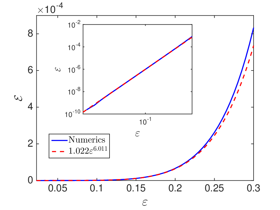
Fig. 4: Plot of the maximum difference (59) of the discrete Schrödinger approximation (3) for varying ε\varepsilon. The dashed line is the best power fit, indicated in the legend. The inset shows the curves in a log scale.

Once a discrete soliton or a discrete breather is found, it is naturally relevant to study their stability.

Let A~j=x^j+i​y^j\tilde{A}_{j}=\hat{x}_{j}+i\hat{y}_{j} be a discrete soliton of the dNLS equation. We determine its linear stability by writing

Aj=A~j+δ⁡(x^j+i​y^j)​eλ​τ.A_{j}=\tilde{A}_{j}+\delta(\hat{x}_{j}+i\hat{y}_{j})e^{\lambda{\tau}}. (55)

Substituting (55) into (3) and linearising around δ=0\delta=0 will yield the eigenvalue problem

λ⁡(x^jy^j)=(−6​ξ​xj​yj−αΔ+Λ−h−3​ξ​(xj2+3​yj2)−Δ−Λ−h+3​ξ​(3​xj2+yj2)6​ξ​xj​yj−α)​(x^jy^j).\lambda\left(\begin{array}[]{c}\hat{x}_{j}\\ \hat{y}_{j}\end{array}\right)=\left(\begin{array}[]{cc}-6\xi{x}_{j}{y}_{j}-\alpha&\Delta+\Lambda-h-3\xi\left({x}_{j}^{2}+3{y}_{j}^{2}\right)\\ -\Delta-\Lambda-h+3\xi\left(3{x}_{j}^{2}+{y}_{j}^{2}\right)&6\xi{x}_{j}{y}_{j}-\alpha\end{array}\right)\left(\begin{array}[]{c}\hat{x}_{j}\\ \hat{y}_{j}\end{array}\right). (56)

In here, the solution A~j\tilde{A}_{j} is said to be linearly stable when all of the eigenvalues λ\lambda have Re(λ)≤0(\lambda)\leq 0 and unstable when there is an eigenvalue with Re(λ)>0(\lambda)>0.

As for discrete breathers of the dKG equation, their linear stability is determined using Floquet theory that can be computed numerically as follows. Let u~j​(t)\tilde{u}_{j}(t) be a breather solution. By defining uj​(t)=u^j​(t)+δ​Yj​(t)u_{j}(t)=\hat{u}_{j}(t)+\delta Y_{j}(t), substituting it into Eq. (1), and linearising the equation around δ=0\delta=0, we obtain the system of linear differential-difference equations

Y˙j=ZjZ˙j=−Yj−3​ξ​u^j2​Yj+ε2​Δ2​Yj−α​Zj+H​cos⁡(2​Ω​t)​Yj.\begin{array}[]{ccl}\dot{Y}_{j}&=&Z_{j}\\ \dot{Z}_{j}&=&-Y_{j}-3\xi\hat{u}_{j}^{2}Y_{j}+\varepsilon^{2}\Delta_{2}Y_{j}-\alpha{Z}_{j}+H\cos\left(2\Omega t\right)Y_{j}.\end{array} (57)

Integrating Eqs. (57) in the numerical domain DD, where now T~=2​π/Ω\widetilde{T}={2\pi}/{\Omega}, and using the standard basis in ℝ2​N\mathbb{R}^{2N}, i.e., {e10,e20,…,e2​N0}\left\{e^{0}_{1},e^{0}_{2},...,e^{0}_{2N}\right\} as the initial condition at t=0t=0, we will obtain a set of solutions at t=T~t=\widetilde{T}, which is our monodromy matrix

M={E1T~,E2T~,…,E2​NT~}∈ℝ2​N×2​N.M=\left\{E^{\widetilde{T}}_{1},E^{\widetilde{T}}_{2},...,E^{\widetilde{T}}_{2N}\right\}\in\mathbb{R}^{2N\times 2N}. (58)

The breather u~j​(t)\tilde{u}_{j}(t) is said to be linearly stable when all the eigenvalues λdKG\lambda_{\text{dKG}} of the monodromy matrix MM, which are known as Floquet multipliers, lie inside or on the unit circle and unstable when there exists at least one λd​K​G\lambda_{dKG} lying outside the unit circle. Note that in the presence of damping, the set of continuous multipliers will lie on a circle of radius e−α​πΩe^{\frac{-\alpha\pi}{\Omega}}, see [21, 22].

Refer to caption
(a)
Refer to caption
(b)
Refer to caption
(c)
Refer to caption
(d)
Fig. 5: Panel (a) shows Floquet multipliers of the breather in Fig. 3a, showing the linear instability of the solution. Panel (b) presents the eigenvalues of the corresponding discrete soliton of DNLS equation (3). Red stars in the panel are the critical multipliers in panel (a), that have been transformed following the relation (60). Panels (c) and (d) compare the real and imaginary part of the critical eigenvalue of the discrete soliton (blue solid line) and the critical multiplier of the corresponding breather of the dKG equation (red dashed line) for varying ε\varepsilon.
Refer to caption
(a)
Refer to caption
(b)
Fig. 6: Time dynamics of the unstable breather (a) and discrete soliton (b) shown in Fig. 3. Note that the time variable in the second panel has been scaled to the original one.

In the following, we focus on breathers and discrete solitons for the same parameter values as in Section 4, i.e., Λ=−3\Lambda=-3, h=−0.5{h}=-0.5, α^=0.1\hat{\alpha}=0.1, and ξ=−1\xi=-1. For ξ=+1\xi=+1, due to the staggering transformation explained briefly in Section 4, discrete breathers of (1) with small amplitudes and discrete solitons of (3) will have exponentially decaying staggered tails.

For our computations, we solve the dKG equation (1) for periodic in time solutions using the number of Fourier modes K=3K=3 and the lattice sites N=50N=50. Larger numbers, i.e., K=9K=9 and N=400N=400, have been used as well to make sure that the results are independent of the lattice size and the number of modes.

We present a breather solution and its time dynamics within one period in Fig. 3 for ε2=0.05\varepsilon^{2}={0.05}. In Fig. 3b, we compare the breather in panel (a) with its corresponding approximation (2), where AjA_{j} is the discrete soliton of Eq. (3). One can note that they are in good agreement.

By defining a maximum difference between breathers of (1) and their approximations (2) using discrete solitons of (3) as

ℰ=sup0≤t≤2​π/Ω∥y⁡(t)∥ℓ2,\mathcal{E}=\sup_{0\leq t\leq 2\pi/\Omega}\lVert y(t)\rVert_{\ell^{2}}, (59)

we depict the error for varying ε\varepsilon in Fig. 4. We also present in the same panel, the best power fit to the numerical results, which interestingly follows the theoretical prediction of the error in Theorem 1, i.e., ∼ε3\sim\varepsilon^{3}.

We have computed the corresponding monodromy matrix for the stability of the solution in Fig. 3a. The Floquet multipliers are plotted in Fig. 5a. We have also solved Eq. (56) for the corresponding discrete soliton of the dNLS equation (3) and plot the eigenvalues λ\lambda in Fig. 5b, where interestingly we obtain that both solutions experience the same type of instability (i.e., oscillatory instability as the critical multipliers and eigenvalues are both complex valued). For the dNLS solitons, this is in agreement with the results of Refs. [10]. For the dKG breather, the instability is similar to that reported in [2]. Moreover, from the time scales that lead to Eqs. (2)–(3), we can obtain the relation between Floquet multipliers λdKG\lambda_{\text{dKG}} of the dKG monodromy matrix (58) and eigenvalues λ\lambda of the dNLS stability matrix (56), i.e.,

λdKG∼eπ​ε2​λ/Ω.\displaystyle\lambda_{\text{dKG}}\sim e^{\pi\varepsilon^{2}\lambda/\Omega}. (60)

Using the transformation, we depict in Fig. 5b the critical multipliers as red stars, where we learn that the localised solutions do not only have the same type of instability, but their critical eigenvalues have relatively comparable magnitudes.

While in Fig. 4 we plot the error made by the dNLS solitons in approximating the dKG breathers, in Figs. 5c and 5d we compare their critical eigenvalues and multipliers for varying ε\varepsilon. We obtain that the breathers and solitons do not necessarily share the same type of stability. In fact, there are intervals of coupling constant ε\varepsilon on which the breathers are stable, even though the corresponding dNLS solitons are unstable. This observation nonetheless does not violate the analytical results in Sections 2–3.

Figures 6a and 6b show the typical dynamics of the oscillatory instability of the breather and its corresponding discrete soliton approximation. We can observe that in both cases the instability destroys localised solutions, i.e., we also obtain qualitative agreement in the instability dynamics.

Finally, for the sake of completeness, we studied the typical dynamics of dKG breathers when they experience an exponential instability, i.e., the critical Floquet multipliers are real. In Figs. 5c and 5d, they are in a finite interval close to the uncoupled limit ε=0\varepsilon=0 and their absolute magnitudes are near unity. Due to these facts, we could not clearly see any instability in our simulations, even after integrating the dKG equation for quite a long while.

References

References

  • [1] B. Denardo, B. Galvin, A. Greenfield, A. Larraza, S. Putterman, and W. Wright, Observations of localized structures in nonlinear lattices: Domain walls and kinks, Physical review letters 68, no. 11 (1992): 1730.
  • [2] J. Cuevas, L.Q. English, P.G. Kevrekidis, and M. Anderson, Discrete breathers in a forced-damped array of coupled pendula: modeling, computation, and experiment, Physical review letters 102, no. 22 (2009): 224101.
  • [3] E. Buks, and M.L. Roukes, Electrically tunable collective response in a coupled micromechanical array, Journal of Microelectromechanical Systems 11, no. 6 (2002): 802-807.
  • [4] B. Denardo, A. Larraza, S. Putterman, and P. Roberts, Nonlinear theory of localized standing waves, Physical review letters 69, no. 4 (1992): 597.
  • [5] S.J. Putterman, and P.H. Roberts, Nonlinear theory of modulated standing waves; domain walls, kinks and breathers, Proceedings of the Royal Society of London. Series A volume 440, no. 1908 (1993): 135-148.
  • [6] R. Lifshitz, and M.C. Cross, Response of parametrically driven nonlinear coupled oscillators with application to micromechanical and nanomechanical resonator arrays, Physical Review B 67, no. 13 (2003): 134302.
  • [7] A.M. Morgante, M. Johansson, G. Kopidakis, Georgios, and S. Aubry, Standing wave instabilities in a chain of nonlinear coupled oscillators, Physica D: Nonlinear Phenomena 162, no. 1-2 (2002): 53-94.
  • [8] D. Pelinovsky, T. Penati, and S. Paleari, Approximation of small-amplitude weakly coupled oscillators by discrete nonlinear Schrödinger equations, Reviews in Mathematical Physics 28, no. 07 (2016): 1650015.
  • [9] D. Hennig, Periodic, quasiperiodic, and chaotic localized solutions of a driven, damped nonlinear lattice, Physical Review E 59, no. 2 (1999): 1637.
  • [10] H. Susanto, Q.E Hoq, and P.G. Kevrekidis, Stability of discrete solitons in the presence of parametric driving, Physical Review E 74, no. 6 (2006): 067601.
  • [11] M. Syafwan, H. Susanto, and S.M. Cox, Discrete solitons in electromechanical resonators, Physical Review E 81, no. 2 (2010): 026207.
  • [12] M. Syafwan, H. Susanto, and S.M. Cox, Solitons in a parametrically driven damped discrete nonlinear Schrödinger equation, In Spontaneous symmetry breaking, Self-Trapping, and Josephson oscillations, pp. 601-638. Springer, Berlin, Heidelberg, 2012.
  • [13] D. Bambusi and A. Ponno, On metastability in FPU, Comm. Math. Phys. 264 (2006): 539-561.
  • [14] B. Bidegaray–Fesquet, E. Dumas, and G. James, From Newton’s cradle to the discrete p-Schrödinger equation, SIAM J. Math. Anal. 45 (2013), 3404–3430.
  • [15] E. Dumas and D.E. Pelinovsky, Justification of the log-KdV equation in granular chains: the case of precompression, SIAM J. Math. Anal. 46 (2014), 4075–4103.
  • [16] G. Friesecke and R.L. Pego, Solitary waves on FPU lattices : I. Qualitative properties, renormalization and continuum limit, Nonlinearity 12 (1999), 1601-1627.
  • [17] G. Schneider and C.E. Wayne, Counter-propagating waves on fluid surfaces and the continuum limit of the Fermi-Pasta-Ulam model, In International Conference on Differential Equations (Berlin, 1999), vol. 1 (eds B Fiedler, K Gröger, J Sprekels), pp. 390–404 (World Sci. Publishing, River Edge, NJ, USA, 2000).
  • [18] W. Dörfler, A. Lechleiter, M. Plum, G. Schneider, and C. Wieners. Photonic Crystals: Mathematical Analysis and Numerical Approximation, Springer Basel, 2011.
  • [19] S. Flach, Computational studies of discrete breathers. In Energy Localization and Transfer (Eds. T. Dauxois et al., World Scientific, 2004), pp. 1-71.
  • [20] S. Flach and A. V. Gorbach, Discrete Breathers, Physics Report 467, 1 (2008).
  • [21] J.L. Marín, F. Falo, P.J. Martínez, and L.M. Floría, Discrete breathers in dissipative lattices, Physical Review E 63, 066603 (2001).
  • [22] P.J. Martínez, M. Meister, L.M. Floría, and F. Falo, Dissipative discrete breathers: Periodic, quasiperiodic, chaotic, and mobile, An Interdisciplinary Journal of Nonlinear Science 13 (2), 610-623 (2003).