Non-Landau Quantum Phase Transitions and nearly-Marginal non-Fermi Liquid
Abstract
Non-fermi liquid and unconventional quantum critical points (QCP) with strong fractionalization are two exceptional phenomena beyond the classic condensed matter doctrines, both of which could occur in strongly interacting quantum many-body systems. This work demonstrates that using a controlled method one can construct a non-Fermi liquid within a considerable energy window based on the unique physics of unconventional QCPs. We will focus on the “nearly-marginal non-Fermi liquid”, defined as a state whose fermion self-energy scales as with close to in a considerable energy window. The nearly-marginal non-fermi liquid is obtained by coupling an electron fermi surface to unconventional QCPs that are beyond the Landau’s paradigm. This mechanism relies on the observation that the anomalous dimension of the order parameter of these unconventional QCPs can be close to , which is significantly larger than conventional Landau phase transitions, for example the Wilson-Fisher fixed points. The fact that justifies a perturbative renormalization group calculation proposed earlier. Various candidate QCPs that meet this desired condition are proposed.
I Introduction
In the past few decades, a consensus has been gradually reached that quantum many-body physics with strong quantum entanglement can be much richer than classical physics driven by thermal fluctuations WEN 1990; Wen 2019. Classical phase transitions usually happen between a disordered phase with high symmetries, and an ordered phase which spontaneously breaks such symmetries. Typical classical phase transitions can be well described by the Landau’s paradigm, but the Landau’s paradigm may or may not apply to quantum phase transitions that happen at zero temperature. Generally speaking, the Landau’s formalism can only describe the quantum phase transition between a direct-product quantum disordered state and a spontaneous symmetry breaking state; but it can no longer describe the quantum phase transition between two states when at least one of the states cannot be adiabatically connected to a direct product states, when this state is a topological order Wen and Wu 1993; nor can the Landau’s paradigm describe generic continuous quantum phase transitions between states with different spontaneous symmetry breakings Senthil et al. 2004b; Senthil et al. 2004a; Jian et al. 2018.
Phenomenologically, in contrast with the ordinary Landau’s transitions, non-Landau transitions often have a large anomalous dimension of order parameters, due to fractionalization or deconfinement of the order parameter Sandvik 2007; Shao et al. 2016; Melko and Kaul 2008; Qin et al. 2017. The ordinary Wilson-Fisher (WF) fixed point in space-time (or three dimensional classical space) has very small anomalous dimensions Calabrese et al. 2003, meaning that the Wilson-Fisher fixed point is not far from the mean field theory. In particular, in the large limit, the anomalous dimension of the vector order parameter of the Wilson-Fisher fixed point is ; while the CPN-1 model, the theory that describes a class of non-Landau quantum phase transition Senthil et al. 2004b; Senthil et al. 2004a, has in the large- limit Kaul and Sachdev 2008. Numerically it was also confirmed that the quantum phase transition between the topological order and the superfluid phase has Isakov et al. 2011; Isakov et al. 2012, as was predicted theoretically. The large anomalous dimension has been used as a strong signature when searching for unconventional QCPs numerically.
In this work we propose that the unique physics described above about the unconventional QCPs with strong fractionalization can be used to construct another broadly observed phenomenon beyond the classic Landau’s theory: the non-Fermi liquid whose fermion self-energy scales with . When , this non-fermi liquid is referred to as marginal fermi liquid Varma et al. 1989. Signature of marginal fermi liquid and nearly-marginal fermi liquid have been observed rather broadly in various materials Löhneysen et al. 2007; Cao et al. 2020; Polshyn et al. 2019. In this work we will focus on the non-Fermi liquid that is “nearly-marginal”, meaning is close to .
We assume that there exists a field in the unconventional QCP that carries zero momentum, and it couples to the fermi surface in the standard way: , where is a flavor matrix of the fermion. We assume that we first solve (or approximately solve) the bosonic part of the theory, the strongly interacting QCP without coupling to the fermi surface, and calculate the anomalous dimension at the QCP:
| (1) |
where . Then the fermion self-energy, the quantity of central interest to us, is computed perturbatively with the boson-fermion coupling .
When the anomalous dimension is close to , we can take with small . Ref. Nayak and Wilczek 1994a; Nayak and Wilczek 1994b; Mross et al. 2010 developed a formalism for the boson-fermion coupled theory with an expansion of , though eventually one needs to extrapolate the calculation to for the problems studied therein Nayak and Wilczek 1994a; Nayak and Wilczek 1994b; Mross et al. 2010, and the convergence of the expansion at is unknown, even if we start with a weak boson-fermion coupling, it would become nonperturbative under renormalization group (RG). But we will demonstrate in the next section that in the cases that we are interested in, is naturally small when is close to , due to the fractionalized nature of many unconventional QCPs. To the leading nontrivial order, our problem can be naturally studied by the previously proposed perturbative formalism with small .
Here we stress that our goal is to construct a scenario in which a non-Fermi liquid state within an energy window can be constructed using a controlled method. Recently many works have taken a similar spirit, and various non-Fermi liquid states especially a state that mimics the strange metal were constructed by deforming the soluble Sachdev-Ye-Kitaev (SYK) and related models Sachdev and Ye 1993; Kitaev 2015; Maldacena and Stanford 2016; Witten 2016; Klebanov and Tarnopolsky 2017. Then within the energy window where the deformation remains perturbative, the system resembles the non-Fermi liquid Song et al. 2017; Patel et al. 2018; Patel and Sachdev 2018; Chowdhury et al. 2018; Wu et al. 2018; Wu et al. 2019a. Our current work also starts with (approximately) soluble strongly interacting bosonic systems (in the sense that the gauge invariant order parameters in these systems are bosonic), and then we turn on perturbation, which in our case is the boson-fermion coupling. We will demonstrate that a non-Fermi liquid can be constructed based on the unique nature of the strongly interacting bosonic system.
II Expansion of
A controlled reliable study of the non-Fermi liquid problem is generally considered as a very challenging problem, one example of the difficulties was discussed in Ref. Lee 2009. Over the years various approximation methods were proposed. We begin by reviewing the expansion developed in Ref. Nayak and Wilczek 1994a; Nayak and Wilczek 1994b; Mross et al. 2010, and demonstrate how perturbation of is naturally justified for some unconventional QCPs. It is often convenient to study interacting fermions with finite density by expanding at one patch of the Fermi surface. The low-energy theory of the fermions expanded at one patch of the fermi surface is
| (2) |
where is perpendicular to the fermion surface and is the tangent direction. The initial value of is , and it will be renormalized by the fermion self-energy. Our main goal is to evaluate the fermion self-energy to the leading nontrivial order of the boson-fermion coupling. We will show that this is equivalent to the leading nontrivial order of . At this order of expansion of , for our purpose it is sufficient to consider a simple “effective action” of :
| (3) |
which will reproduce the correlation function of , assuming we have fully solved the interacting bosonic system first.
When the boson-fermion coupling is zero, i.e., , the system is at a Gaussian fixed point with the following scaling dimensions of spacetime coordinates and fields
| (4) | |||
| (5) | |||
| (6) |
We then turn on the boson-fermion interaction
| (7) |
and consider the perturbative RG at the Gaussian fixed point. We find that the scaling dimension of is , hence it is weakly relevant if is naturally small, and it may flow to a weakly coupled new fixed point in the infrared which facilitates perturbative calculations with expansion of . Indeed, the beta function of at the leading order of was derived in Ref. Nayak and Wilczek 1994a; Nayak and Wilczek 1994b; Mross et al. 2010:
| (8) |
Thus there is a fixed point at weak coupling , where the parameter .
Under the rescaling , namely after integrating out the short scale degrees of freedom, the fermion acquires a one-loop self-energy
| (9) | |||
| (10) | |||
| (11) | |||
| (12) | |||
| (13) |
In the boson correlation function, and are irrelevant compared with , hence we first integrate over , and the fermion propagator contributes a factor . We then perform the integral and finally integrate over the momentum shell . The last integral is evaluated at , which is valid at the leading order perturbation of . This procedure leads to
| (14) |
Combining the calculations above, at the fixed point , the renormalized in the Fermion Green’s function reads
| (15) |
The fermion self-energy, hence the decay rate of the fermion, scales in the same way as Eq. 15. The calculation above gives a nearly-marginal non-Fermi liquid behavior for small but finite . For small such as the cases in the Wilson-Fisher fixed points, the calculation of the scaling of fermion self-energy is not reliable with the leading order expansion of described above.
Here we stress that, our main purpose is to compute , or the fermion self-energy to the leading order of boson-fermion coupling , assuming a weak initial coupling . At higher order expansion of the boson-fermion coupling, corrections to the boson field self-energy (for example the standard RPA diagram) from the boson-fermion coupling needs to be considered. The RPA diagram is proportional to . Several parameters can be tuned, including the weak coupling fixed point value of , to make this term weak enough to allow an energy window where the calculations in this section apply. At the elementary level, we need the terms in Eq. 3 to dominate the RPA effect . A field at momentum should correspond to energy scale . For Eq. 3 at to dominate the RPA effect, we need , or . If we start with a weak initial bare coupling constant , and also hence the fixed point value of is also perturbative, there is a sufficiently large energy window for our result. Tuning the parameter and can further expand the energy window. A full analysis of the term in the bosonic sector of the theory in the infrared limit requires more detailed analysis because is a composite operator in the field theories discussed in the next section.
III Candidate unconventional QCPs
(1) Bosonic-QED-Chern-Simons theory
In the following we will discuss candidate QCPs which suffice the desired condition , or . When we study the pure bosonic sector of the theory, we ignore the coupling to the fermions, assuming the boson-fermion coupling is weak, which is self-consistent with the conclusion in the previous review section that the boson-fermion interaction will flow to a weakly coupled fixed point . As we stated in the previous section, we will start with a weak boson-fermion coupling , and eventually we only compute the fermion self-energy to the leading nontrivial order of the fixed point . In the purely bosonic theory, the scaling of the space-time has the standard Lorentz invariance. To avoid confusion, we use “” to represent scaling dimensions under the scaling Eq. 6 of the one-patch theory in the previous section, and “” represent the scaling dimension in the Lorentz invariant purely bosonic theory. At a QCP, multiple operators will become “critical”, namely multiple operators can have power-law correlation. We will demand that the operator with the strongest correlation (smallest scaling dimension) satisfy the desired condition, since this is the operator that provides the strongest scattering with the electrons.
We consider bosonic quantum electrodynamics (QED) with flavors of bosons coupled to a noncompact gauge field with a Chern-Simons term:
| (16) | |||||
| (18) | |||||
| (20) |
The following operators are gauge invariant composite fields, which we assume are all at zero momentum:
| (21) |
Potential applications of this field theory to strongly correlated systems will be discussed later.
To compute their scaling dimensions, we introduce two Hubbard-Stratonovich(HS) fields to decouple the quartic potentials:
| (22) | |||||
| (24) | |||||
| (26) |
We will consider the following two scenarios: (1) , where is fully suppressed and the system has a full symmetry, where the is the “topological symmetry” that corresponds to the conservation of the gauge flux; and (2) when the symmetry is broken down to , where the is the symmetry within the Pauli matrix space in Eq. 21.
In scenario (1) with a full symmetry, at the critical point , the field acquires a self-energy in the large limit
| (27) |
Hence the propagator of field in the large limit reads
| (28) |
Similarly, for the gauge field, the self-energy in the large limit is
| (29) | |||||
| (31) |
When combined with the Chern-Simons term, in the Landau gauge, the gauge field has the following large propagator Wen and Wu 1993
| (32) |
where
| (33) |
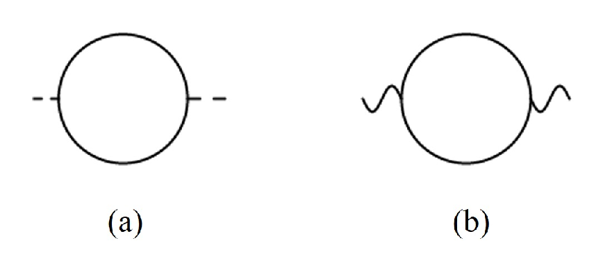
After introducing the HS fields, the scaling dimension of the composite operator of the original field theory Eq. 20 is “transferred” to the scaling dimension of the HS fields . To the order of , the Feynman diagrams in Fig. 2 contribute to the self energy, which was computed in Ref. Wen and Wu 1993.

But it is evident that in the large limit, the scaling dimension of (and the scaling dimension of operator of the original field theory Eq. 20) is , hence it does not meet the desired condition. When couples to the Fermi surface, the boson-fermion coupling will be irrelevant in the one patch theory discussed in the previous section according to the scaling of space-time Eq. 6.
The scaling dimension of equal to each other with a full symmetry, and unlike , they have scaling dimension in the large limit. The corrections to their anomalous dimensions come from diagram in Fig. 2, or equivalently through the standard momentum shell RG:
| (34) |
Ref. Kaul and Sachdev 2008 and references therein have computed scaling dimensions of gauge invariant operators for theories with matter fields coupled with a gauge field, without a Chern-Simons term. Our result is consistent with these previous references, since , which is the result of the CPN-1 model with a noncompact gauge field. Also, in the limit of , our result is consistent with Ref. Kaul and Sachdev 2008 when the fermion component is taken to be infinity, since both limits suppress the gauge field fluctuation completely. In general operators have stronger correlations than , hence they will make stronger contributions to scattering when coupled with the fermi surface. As an example, the anomalous dimension of with reads
| (35) |
which is reasonably close to even for the most physically relevant case with .
In scenario (2) we should keep both and in the calculation, and both (operator and in theory Eq. 20) have scaling dimension 2 in the large limit Benvenuti and Khachatryan 2019. Now has the strongest correlation, and at the order of , its scaling dimension reads:
| (36) |
When , its anomalous dimension reads
| (37) |
which is always very close to . Using the formalism reviewed in the previous section, by coupling to , the fermion self-energy would scale as for .
The field theory Eq. 20 describes a quantum phase transition from a topological order with Abelian anyons to an ordered phase that spontaneously breaks the global flavor symmetry. The flavor symmetry can be either a full symmetry (scenario 1) or (scenario 2). So far we have assumed that the gauge invariant have zero momentum, hence they cannot be the ordinary antiferromagnetic Néel order parameter. They must be translational invariant order parameters with nontrivial representation under the internal symmetry group, for example they could be the quantum spin Hall order parameter for .
The topological order described by the Chern-Simons theory with , is the most studied state in condensed matter theory. This topological order is the or equivalently the topological order with semionic anyons. It is the most natural topological order that can be constructed from the slave particle formalism Wen 2002. And recently it was conjectured that this topological order is also related to the parent state of the cuprates high temperature superconductor Samajdar et al. 2019 motivated by the giant thermal Hall signal observed Grissonnanche et al. 2019.
Another interesting scenario is when , and . In this case Eq. 20 is the same field theory as the easy-plane deconfined QCP between the inplane antiferromagnetic Néel order and the valence bond solid state on the square lattice. Recent numerical studies have shown that this quantum phase transition may be continuous, and the scaling dimension of both and are fairly close to based on numerical results Qin et al. 2017; Karthik and Narayanan 2016. It has been proposed that this field theory is self-dual Motrunich and Vishwanath 2004, and it is dual to the transition between the bosonic symmetry protected topological (SPT) phase and the trivial phase Wang et al. 2017; Potter et al. 2017, which is directly describe by a noncompact QED with flavors of Dirac fermion matter fields Grover and Vishwanath 2013; Lu and Lee 2014. The tuning parameter for this topological transition is instead coupled to . Hence this SPT-trivial transition is also a candidate quantum phase transition which meets the desired criterion proposed in our paper that leads to a nearly-marginal fermi liquid. But in these cases there are other fields (for example the inplane Néel order parameter) with smaller scaling dimensions, and we need to assume that these operators carry finite lattice momentum hence couple to the Fermi surface differently.
(2) Gross-Neveu-Yukawa QCP
Another candidate QCP that likely suffices the desired condition is the Gross-Neveu-Yukawa QCP with flavors of Dirac fermion:
| (38) | |||||
| (40) |
At the critical point , both and flows to a fixed point. In our context, the QCP describes a bosonic or spin system, hence is viewed as a fermionic slave particle of spin, the spinon, and we assume that is coupled to a gauge field, namely the system is a spin liquid with fermionic spinons. But the dynamical gauge field does not lead to extra singular corrections to low energy correlation functions of gauge invariant operators, hence the universality class of Eq. 40 is still identical to the Gross-Neveu-Yukawa (GNY) theory, as long as we only focus on gauge invariant operators.
The GNY QCP can still be solved in the large limit, and the cases with finite can approached through a expansion. At the GNY QCP coupled with a gauge field, the gauge invariant operator with the lowest scaling dimension is , and its scaling dimension can be found in Ref. Boyack et al. 2019 and references therein:
| (41) |
Other gauge invariant operators such as with a matrix have much larger scaling dimension at the GNY QCP, for example in the large limit. If we replace the gauge field by a gauge field, the gauge fluctuation will enhance the correlation of , hence increases compared with the situation with only a gauge field. Hence a GNY QCP with a gauge field is less desirable according to our criterion.
The GNY QCP coupled with a gauge field can be realized in various lattice model Hamiltonians for quantum antiferromagnet. For example, for spin systems on the triangular lattice with a self-conjugate representation on each site, using the fermionic spinon formalism, when there is a flux through half of the triangles, there are components of Dirac fermions at low energy Lu 2016. quantum magnet may be realized in transition metal oxides with orbital degeneracies Pati et al. 1998; Li et al. 1998; Tokura and Nagaosa 2000, and also cold atom systems with large hyperfine spins Wu et al. 2003; Wu 2005; WU 2006; Gorshkov et al. 2009. Recently it was also proposed that an approximate quantum antiferromagnet can be realized in some of the recently discovered Moiré systems Xu and Balents 2018; Wu et al. 2019b; Schrade and Fu 2019, and a quantum antiferromagnet on the triangular lattice may realize the gauged GNY QCP with (with lower spatial symmetry compared with systems as was pointed out in Ref. Zhang and Mao 2019). On the other hand, a spin systems on the honeycomb lattice can potentially realize the GNY QCP with (with zero flux through the hexagon) or (with flux through the hexagon).
The operator is odd under time-reversal and spatial reflection, hence physically corresponds to the spin chirality order. Hence the gauged GNY QCP is a quantum phase transition between a massless spin liquid and a chiral spin liquid.
Non-Fermi liquid is often observed only at a finite temperature/energy window in experiments. At the infrared limit, the non-Fermi liquid is usually preempted by other instabilities, for example a dome of superconductor Metlitski et al. 2015; Lederer et al. 2015; Rech et al. 2006. In Ref. Metlitski et al. 2015 the instability of non-Fermi liquid towards the superconductor dome was systematically studied in the framework of the expansion. According to Ref. Metlitski et al. 2015, when is an order parameter at zero momentum, at the superconductor instability will occur at an exponentially suppressed temperature/energy scale , where is the bare boson-fermion coupling constant. In our case the estimate of the superconductor instability is complicated by the fact that is a composite field, but the qualitative exponentially-suppressed form of is not expected to change because is still at most a marginally relevant coupling. When , the imaginary part of the fermi self-energy (the inverse of quasi-particle life-time) scales linearly with . Because the bare electron dispersion has no imaginary part at all, the imaginary part of the self-energy should be much easier to observe compared with the real part, assuming other scattering mechanisms of the fermions are weak enough. The scaling behavior of the fermion self-energy is also observable numerically like Ref. Xu et al. 2020. This linear scaling behavior of the imaginary part of self-energy is observable for fermionic excitations at energy scale , . Hence above the superconductor energy scale , the non-Fermi liquid behavior is observable. This result should still hold for small enough . 11 1 In Ref. Metlitski et al. 2015, the non-Fermi liquid energy scale is defined as the energy scale where the fermi velocity is renormalized strongly from its bare value, hence was defined based on the real part of the fermion self-energy. In other words the was defined as the scale where the real part of self-energy dominates the bare energy in the Green’s function. But since the bare dispersion of fermion is difficult to observe, and the bare fermion energy has no imaginary part at all, we prefer to use the imaginary part of fermion self-energy as a characteristic definition of non-Fermi liquid state.
IV Conclusion
In this work we proposed a mechanism based on which a nearly marginal non-fermi liquid can be constructed with a controlled method in an energy window. This mechanism demonstrates that two exceptional phenomena beyond the standard Landau’s paradigm, the non-Landau quantum phase transitions and the non-fermi liquid may be connected: a non-Landau quantum phase transition can have a large anomalous dimension , which physically justifies and facilitates a perturbative calculation of the Boson-Fermion coupling fixed point. Several candidate QCPs that suffice this condition were proposed, including topological transitions from Abelian topological orders to an ordered phase, and a Gross-Neveu-Yukawa transition of spin liquids.
We would like to compare our construction of non-fermi liquid states and the constructions based on the SYK related models. In the constructions based on SYK-like models, the existence of a strange-metal like phase was based on the fact that in the soluble limit, in the SYK model the scaling dimension of fermion is (scaling with time only). But since the definition of the electric current operator in these constructions is proportional to the perturbation away from the SYK model, the current-current correlation function and the electrical conductivity is small in the energy window where the construction applies. Recently an improved construction was proposed which can produce the Planckian metal observed in cuprates materials Patel and Sachdev 2019. In our construction, since the boson-fermion coupling will flow to a weakly coupled fixed point, the scattering rate of the fermion due to the boson-fermion coupling is expected to be low. We will further study if a Planckian metal like state can be constructed by developing our current approach. In this future exploration, a mechanism of momentum relaxation, for instance the disorder, or Umklapp process, needs to be introduced.
This work is supported by NSF Grant No. DMR-1920434, the David and Lucile Packard Foundation, and the Simons Foundation.
References
- WEN (1990) X. G. WEN, International Journal of Modern Physics B 04, 239 (1990), eprint https://doi.org/10.1142/S0217979290000139, URL https://doi.org/10.1142/S0217979290000139.
- Wen (2019) X.-G. Wen, Science 363 (2019), ISSN 0036-8075, eprint https://science.sciencemag.org/content/363/6429/eaal3099.full.pdf, URL https://science.sciencemag.org/content/363/6429/eaal3099.
- Wen and Wu (1993) X.-G. Wen and Y.-S. Wu, Phys. Rev. Lett. 70, 1501 (1993), URL https://link.aps.org/doi/10.1103/PhysRevLett.70.1501.
- Jian et al. (2018) C.-M. Jian, A. Thomson, A. Rasmussen, Z. Bi, and C. Xu, Phys. Rev. B 97, 195115 (2018), URL https://link.aps.org/doi/10.1103/PhysRevB.97.195115.
- Senthil et al. (2004a) T. Senthil, L. Balents, S. Sachdev, A. Vishwanath, and M. P. A. Fisher, Phys. Rev. B 70, 144407 (2004a).
- Senthil et al. (2004b) T. Senthil, A. Vishwanath, L. Balents, S. Sachdev, and M. P. A. Fisher, Science 303, 1490 (2004b).
- Melko and Kaul (2008) R. G. Melko and R. K. Kaul, Phys. Rev. Lett. 100, 017203 (2008), URL https://link.aps.org/doi/10.1103/PhysRevLett.100.017203.
- Qin et al. (2017) Y. Q. Qin, Y.-Y. He, Y.-Z. You, Z.-Y. Lu, A. Sen, A. W. Sandvik, C. Xu, and Z. Y. Meng, Phys. Rev. X 7, 031052 (2017), URL https://link.aps.org/doi/10.1103/PhysRevX.7.031052.
- Sandvik (2007) A. W. Sandvik, Phys. Rev. Lett. 98, 227202 (2007), URL https://link.aps.org/doi/10.1103/PhysRevLett.98.227202.
- Shao et al. (2016) H. Shao, W. Guo, and A. W. Sandvik, Science 352, 213 (2016), ISSN 0036-8075, eprint https://science.sciencemag.org/content/352/6282/213.full.pdf, URL https://science.sciencemag.org/content/352/6282/213.
- Calabrese et al. (2003) P. Calabrese, A. Pelissetto, and E. Vicari, arXiv:cond-mat/0306273 (2003).
- Kaul and Sachdev (2008) R. K. Kaul and S. Sachdev, Phys. Rev. B 77, 155105 (2008), URL https://link.aps.org/doi/10.1103/PhysRevB.77.155105.
- Isakov et al. (2011) S. V. Isakov, M. B. Hastings, and R. G. Melko, Nature Physics 7, 772 (2011).
- Isakov et al. (2012) S. V. Isakov, M. B. Hastings, and R. G. Melko, Science 335, 193 (2012).
- Varma et al. (1989) C. M. Varma, P. B. Littlewood, S. Schmitt-Rink, E. Abrahams, and A. E. Ruckenstein, Phys. Rev. Lett. 63, 1996 (1989), URL https://link.aps.org/doi/10.1103/PhysRevLett.63.1996.
- Cao et al. (2020) Y. Cao, D. Chowdhury, D. Rodan-Legrain, O. Rubies-Bigorda, K. Watanabe, T. Taniguchi, T. Senthil, and P. Jarillo-Herrero, Phys. Rev. Lett. 124, 076801 (2020), URL https://link.aps.org/doi/10.1103/PhysRevLett.124.076801.
- Löhneysen et al. (2007) H. v. Löhneysen, A. Rosch, M. Vojta, and P. Wölfle, Rev. Mod. Phys. 79, 1015 (2007), URL https://link.aps.org/doi/10.1103/RevModPhys.79.1015.
- Polshyn et al. (2019) H. Polshyn, M. Yankowitz, S. Chen, Y. Zhang, K. Watanabe, T. Taniguchi, C. R. Dean, and A. F. Young, arXiv:1902.00763 (2019).
- Mross et al. (2010) D. F. Mross, J. McGreevy, H. Liu, and T. Senthil, Phys. Rev. B 82, 045121 (2010), URL https://link.aps.org/doi/10.1103/PhysRevB.82.045121.
- Nayak and Wilczek (1994a) C. Nayak and F. Wilczek, Nuclear Physics B 417, 359 (1994a), ISSN 0550-3213, URL http://www.sciencedirect.com/science/article/pii/055032139490%4774.
- Nayak and Wilczek (1994b) C. Nayak and F. Wilczek, Nuclear Physics B 430, 534 (1994b), ISSN 0550-3213, URL http://www.sciencedirect.com/science/article/pii/055032139490%1589.
- Kitaev (2015) A. Kitaev, A simple model of quantum holography, http://online.kitp.ucsb.edu/online/entangled15/kitaev/ (2015), Talks at KITP, April 7, 2015 and May 27, 2015.
- Klebanov and Tarnopolsky (2017) I. R. Klebanov and G. Tarnopolsky, Phys. Rev. D 95, 046004 (2017), URL https://link.aps.org/doi/10.1103/PhysRevD.95.046004.
- Maldacena and Stanford (2016) J. Maldacena and D. Stanford, Phys. Rev. D 94, 106002 (2016), eprint 1604.07818.
- Sachdev and Ye (1993) S. Sachdev and J. Ye, Physical Review Letters 70, 3339 (1993), eprint cond-mat/9212030.
- Witten (2016) E. Witten, ArXiv e-prints (2016), eprint 1610.09758.
- Chowdhury et al. (2018) D. Chowdhury, Y. Werman, E. Berg, and T. Senthil, Phys. Rev. X 8, 031024 (2018), URL https://link.aps.org/doi/10.1103/PhysRevX.8.031024.
- Patel et al. (2018) A. A. Patel, J. McGreevy, D. P. Arovas, and S. Sachdev, Phys. Rev. X 8, 021049 (2018), URL https://link.aps.org/doi/10.1103/PhysRevX.8.021049.
- Patel and Sachdev (2018) A. A. Patel and S. Sachdev, Phys. Rev. B 98, 125134 (2018), URL https://link.aps.org/doi/10.1103/PhysRevB.98.125134.
- Song et al. (2017) X.-Y. Song, C.-M. Jian, and L. Balents, Phys. Rev. Lett. 119, 216601 (2017), URL https://link.aps.org/doi/10.1103/PhysRevLett.119.216601.
- Wu et al. (2019a) X.-C. Wu, C.-M. Jian, and C. Xu, Phys. Rev. B 100, 075101 (2019a), URL https://link.aps.org/doi/10.1103/PhysRevB.100.075101.
- Wu et al. (2018) X. Wu, X. Chen, C.-M. Jian, Y.-Z. You, and C. Xu, Phys. Rev. B 98, 165117 (2018), URL https://link.aps.org/doi/10.1103/PhysRevB.98.165117.
- Lee (2009) S.-S. Lee, Phys. Rev. B 80, 165102 (2009), URL https://link.aps.org/doi/10.1103/PhysRevB.80.165102.
- Benvenuti and Khachatryan (2019) S. Benvenuti and H. Khachatryan, Journal of High Energy Physics 2019, 214 (2019), ISSN 1029-8479, URL https://doi.org/10.1007/JHEP05(2019)214.
- Wen (2002) X.-G. Wen, Phys. Rev. B 65, 165113 (2002), URL https://link.aps.org/doi/10.1103/PhysRevB.65.165113.
- Samajdar et al. (2019) R. Samajdar, M. S. Scheurer, S. Chatterjee, H. Guo, C. Xu, and S. Sachdev, Nature Physics 15, 1290 (2019).
- Grissonnanche et al. (2019) G. Grissonnanche, A. Legros, S. Badoux, E. Lefrançois, V. Zatko, M. Lizaire, F. Laliberté, A. Gourgout, J.-S. Zhou, S. Pyon, et al., Nature 571, 376 (2019).
- Karthik and Narayanan (2016) N. Karthik and R. Narayanan, Phys. Rev. D 94, 065026 (2016), URL https://link.aps.org/doi/10.1103/PhysRevD.94.065026.
- Motrunich and Vishwanath (2004) O. I. Motrunich and A. Vishwanath, Phys. Rev. B 70, 075104 (2004).
- Potter et al. (2017) A. C. Potter, C. Wang, M. A. Metlitski, and A. Vishwanath, Phys. Rev. B 96, 235114 (2017), URL https://link.aps.org/doi/10.1103/PhysRevB.96.235114.
- Wang et al. (2017) C. Wang, A. Nahum, M. A. Metlitski, C. Xu, and T. Senthil, Phys. Rev. X 7, 031051 (2017), URL https://link.aps.org/doi/10.1103/PhysRevX.7.031051.
- Grover and Vishwanath (2013) T. Grover and A. Vishwanath, Phys. Rev. B 87, 045129 (2013).
- Lu and Lee (2014) Y.-M. Lu and D.-H. Lee, Phys. Rev. B 89, 195143 (2014), URL https://link.aps.org/doi/10.1103/PhysRevB.89.195143.
- Boyack et al. (2019) R. Boyack, A. Rayyan, and J. Maciejko, Phys. Rev. B 99, 195135 (2019), URL https://link.aps.org/doi/10.1103/PhysRevB.99.195135.
- Lu (2016) Y.-M. Lu, Phys. Rev. B 93, 165113 (2016), URL https://link.aps.org/doi/10.1103/PhysRevB.93.165113.
- Li et al. (1998) Y. Q. Li, M. Ma, D. N. Shi, and F. C. Zhang, Phys. Rev. Lett. 81, 3527 (1998), URL https://link.aps.org/doi/10.1103/PhysRevLett.81.3527.
- Pati et al. (1998) S. K. Pati, R. R. P. Singh, and D. I. Khomskii, Phys. Rev. Lett. 81, 5406 (1998), URL https://link.aps.org/doi/10.1103/PhysRevLett.81.5406.
- Tokura and Nagaosa (2000) Y. Tokura and N. Nagaosa, Science 288, 462 (2000), ISSN 0036-8075, eprint https://science.sciencemag.org/content/288/5465/462.full.pdf, URL https://science.sciencemag.org/content/288/5465/462.
- Gorshkov et al. (2009) A. V. Gorshkov, M. Hermele, V. Gurarie, C. Xu, P. S. Julienne, J. Ye, P. Zoller, E. Demler, M. D. Lukin, and A. M. Rey, Nature Physics 6, 289 (2009).
- Wu (2005) C. Wu, Phys. Rev. Lett. 95, 266404 (2005), URL https://link.aps.org/doi/10.1103/PhysRevLett.95.266404.
- WU (2006) C. WU, Modern Physics Letters B 20, 1707 (2006), eprint https://doi.org/10.1142/S0217984906012213, URL https://doi.org/10.1142/S0217984906012213.
- Wu et al. (2003) C. Wu, J.-p. Hu, and S.-c. Zhang, Phys. Rev. Lett. 91, 186402 (2003), URL https://link.aps.org/doi/10.1103/PhysRevLett.91.186402.
- Schrade and Fu (2019) C. Schrade and L. Fu, Phys. Rev. B 100, 035413 (2019), URL https://link.aps.org/doi/10.1103/PhysRevB.100.035413.
- Wu et al. (2019b) X.-C. Wu, A. Keselman, C.-M. Jian, K. A. Pawlak, and C. Xu, Phys. Rev. B 100, 024421 (2019b), URL https://link.aps.org/doi/10.1103/PhysRevB.100.024421.
- Xu and Balents (2018) C. Xu and L. Balents, Phys. Rev. Lett. 121, 087001 (2018), URL https://link.aps.org/doi/10.1103/PhysRevLett.121.087001.
- Zhang and Mao (2019) Y.-H. Zhang and D. Mao, arXiv e-prints arXiv:1906.10132 (2019), eprint 1906.10132.
- Lederer et al. (2015) S. Lederer, Y. Schattner, E. Berg, and S. A. Kivelson, Phys. Rev. Lett. 114, 097001 (2015), URL https://link.aps.org/doi/10.1103/PhysRevLett.114.097001.
- Metlitski et al. (2015) M. A. Metlitski, D. F. Mross, S. Sachdev, and T. Senthil, Phys. Rev. B 91, 115111 (2015), URL https://link.aps.org/doi/10.1103/PhysRevB.91.115111.
- Rech et al. (2006) J. Rech, C. Pépin, and A. V. Chubukov, Phys. Rev. B 74, 195126 (2006), URL https://link.aps.org/doi/10.1103/PhysRevB.74.195126.
- Xu et al. (2020) X. Y. Xu, A. Klein, K. Sun, A. V. Chubukov, and Z. Y. Meng, arXiv e-prints arXiv:2003.11573 (2020), eprint 2003.11573.
- Patel and Sachdev (2019) A. A. Patel and S. Sachdev, Phys. Rev. Lett. 123, 066601 (2019), URL https://link.aps.org/doi/10.1103/PhysRevLett.123.066601.