Uncertainty and Sensitivity Analyses Methods for Agent-Based Mathematical Models: An Introductory Review
Sara Hamis1,2, Stanislav Stratiev3, Gibin G Powathil2.
1 School of Mathematics and Statistics, University of St Andrews, St Andrews KY16 9SS, Scotland.
2 Department of Mathematics, College of Science, Swansea University, Swansea, SA1 8EN, United Kingdom.
3 Department of Physics, College of Science, Swansea University, Swansea, SA2 8PP, United Kingdom.
Abstract
Multiscale, agent-based mathematical models of biological systems are often associated with model uncertainty and sensitivity to parameter perturbations. Here, three uncertainty and sensitivity analyses methods, that are suitable to use when working with agent-based models, are discussed. These methods are namely Consistency Analysis, Robustness Analysis and Latin Hypercube Analysis. This introductory review discusses origins, conventions, implementation and result interpretation of the aforementioned methods. Information on how to implement the discussed methods in MATLAB is included.
1 Introduction
Mathematical models of biological systems are abstractions of highly complex reality. It follows that parameters used in such models often are associated with some degree of uncertainty, where the uncertainty can be derived from various origins. Epistemic uncertainty refers to uncertainty resulting from limited knowledge about the biological system at hand, whilst aleatory uncertainty stems from naturally occurring stochasticity, intrinsic to biological systems [23, 1, 15]. Model parameters may thus be naturally stochastic, theoretically unknown, and unfeasible or impossible to measure precisely (or at all). Further magnifying the contributions of uncertainty in mathematical models of biological systems, in particular, is the fact that one parameter in the mathematical model may correspond to a multitude of underlying biological mechanisms and factors in the real, biological system. This is especially true for minimal parameter models, i.e. mathematical models that aspire to be as non-complex as possible whilst still capturing all biological details of interest [8]. In this review, we focus our attention on uncertainty and sensitivity analyses techniques that are suitable for use with agent-based models. A mathematical, agent-based model comprises several distinct agents that may interact with each other and their environment. In an agent-based tumour model, for example, an agent typically corresponds to one tumour cell or a group of tumour cells. This naturally allows for heterogeneity amongst tumour cells, which is useful as tumour heterogeneity is associated with many complications involved in modelling (and treating) solid tumours. Accordingly, many modellers in the field of mathematical oncology choose to work with agent-based models [24].
There already exist multiple method papers that describe how to perform uncertainty and sensitivity analyses when working with agent-based models, authors Alden et al. even provide a free R-based software package (Spartan [1]) that enables the user to perform different such methods, including the three methods discussed in this review. However, as these methods have been developed across multiple research fields, both inside and outside of the natural sciences, it is difficult to find one comprehensive review that discusses not only how to perform these methods, but also where these methods come from, and why certain conventions are proposed and/or used.
To this end, we have in this review gathered such information for three uncertainty and sensitivity analyses techniques, namely Consistency Analysis, Robustness Analysis and Latin Hypercube Analysis.
Our aim is that this will allow the reader to better evaluate uncertainty and sensitivity analyses presented by other authors, and encourage the reader to consider performing these methods when suitable.
In order to understand the impact that parameter uncertainty and parameter perturbations have on results produced by a mathematical model, uncertainty and sensitivity analyses can be used.
A mathematical model that comprises a set of uncertain model parameters (or inputs), is able to produce a range of possible responses (or outputs).
Uncertainty analysis assesses the range of these outputs overall, and provides information regarding how certain (or uncertain) we should be with our model results, and the conclusions that we draw from them [2].
Sensitivity analysis describes the relationship between uncertainty in inputs and uncertainty in outputs. It can be used to identify which sources of input uncertainty (i.e. which model parameters) significantly influence the uncertainty in the output and, equally importantly, which do not [2].
Assessing how sensitive the output is to small input perturbations is a healthy way to scrutinise our mathematical models [14]. Moreover, for a well-formulated model, knowledge regarding how input uncertainty influences output uncertainty can yield insight into the biological system that has not yet been empirically observed [1]. Furthermore, if the uncertainty in some input parameter is shown to not affect output uncertainty, the modeller may consider fixing that parameter, and thus reducing model complexity in accordance with a minimal-parameter modelling approach.
In local sensitivity analysis techniques, model parameters (inputs) are perturbed one at a time whilst other parameters remain fixed at their calibrated value. In global sensitivity analysis techniques, all model parameters are simultaneously perturbed [4].
There exist several sensitivity and uncertainty analyses techniques, but here we will focus on three such techniques that are suitable to use in conjunction with agent-based mathematical models.
These techniques are namely Consistency Analysis, Robustness Analysis and Latin Hypercube Analysis, which all answer important, and complementary, questions about mathematical models and their corresponding in silico responses [23, 1].
![[Uncaptioned image]](1911.08429v3/saquestions.png)
Note that Consistency Analysis is only meaningful when analysing models with stochastic variables.
The statistical techniques described in this review have been developed and applied across multiple academic disciplines, both inside and outside of the natural sciences. Consequently, terminology and notations vary in the literature. The aim of this review is to combine pertinent literature from various academic fields whilst keeping terminology and mathematical notations consistent, unambiguous and tailored towards a mathematical and scientific audience. Therefore, when needed, certain algorithms from the literature are here reformulated into expressions that a mathematician would consider to be conventional. This review is intended to provide gentle, yet comprehensive, instructions to the modeller wanting to perform uncertainty and sensitivity analyses on agent-based models. Thorough directions on how to perform Consistency Analysis (Section 3), Robustness Analysis (Section 4) and Latin Hypercube Sampling and Analysis (Section 5) are provided. Consistency Analysis utilises the A-measure of stochastic superiority, which is therefore discussed in Section 2. Throughout this review, we have included some historical information that elucidates why certain statistical conventions are used. Each section also contains pictorial, step-by-step instructions on how to perform the aforementioned techniques. Worked examples of all methods discussed in this review are provided in Section 6. These worked examples use in silico data produced in a previous agent-based, multiscale, mathematical oncology study [9].
Methods outside the scope of this review
Note that there exist other uncertainty and sensitivity analyses techniques, suitable for agent-based models, that are outside the scope of this review. For example, Bayesian inference is a statistical technique that uses Bayes theorem, prior beliefs and observed data to infer input parameter values and their associated uncertainties [12]. When this inference is difficult to calculate, computational methods such as Approximate Bayesian Computation (ABC) [13] or, if the model is highly computationally expensive, Approximate Approximate Bayesian Computation (AABC) [3] can be used to perform inference on input model parameters. The Sobol method is a variance-based sensitivity analysis method that, using Monte-Carlo multidimensional integration, allows for the evaluation of each individual parameter’s fractional contribution to the output variance [31]. Another global, variance based sensitivity analysis method that enables quantification of the input parameter’s fractional contributions to the output variance is Fourier amplitude sensitivity testing (FAST) which uses an underlying algorithm that involves Fourier decomposition [26]. Although the Sobol method and FAST use different underlying techniques, they both allow us to say that “input parameter contributes percent to the output variance”. Newer sensitivity analysis methods and tools tend to take advantage of the current abundance of computing power. The recently introduced MASSIVE (Massively parallel Agent-based Simulations and Subsequent Interactive Visualization-based Exploration) methodology, for example, combines parallel computing and interactive data visualisation to produce a graphical user interface that provides an overview of input-output relations for a broad input parameter range [22].
2 The A-measure of stochastic superiority
2.1 The Common Language Statistics
In 1992, McGraw and Wong introduced the common language statistics () as an intuitive way to compare two distributions of data [18]. The was initially introduced as a tool to compare data from normal distributions, but was later on approximated for use on any continuous distributions. The describes the probability that a random data sample from one of the distributions is greater than a random data sample from the other distribution. For example, if we have two continuous data distributions and , and we are comparing the distributions with respect to some variable , then the is simply given by
| (1) |
where standard probability notations have been used so that denotes the probability that a random data sample from distribution is greater than a random data sample from distribution [18]. Thus the subscript of here signifies the distribution from which the data sample was taken.
2.2 The A-measure of stochastic superiority
The was developed to compare continuous data distributions, but Vargha and Delaney [29] introduced the A-measure of stochastic superiority (or A-measure for short) as a generalisation of the that can directly be applied to compare both continuous and discrete distributions of variables that are at least ordinally scaled. When comparing two distributions and , with respect to the variable , the A-measure is given by
| (2) |
where denotes the probability that a random data sample from distribution is equal to a random data sample from distribution .
By comparing Equations 1 and 2, it is clear that in the continuous case, where , the A-measure reduces to the .
If two distributions that are identical with respect to the variable are compared, then and we say that the distributions and are stochastically equal with respect to the variable .
On the other hand, if , then we say that the distribution is stochastically greater than distribution , and accordingly, that distribution is stochastically smaller than distribution [29].
If distribution is stochastically greater than distribution with respect to the variable , it simply occurs more often that the sample is greater than the sample when two random samples and are compared.
These definitions of stochastic relationships (stochastically equal to, stochastically greater than, stochastically smaller than), used by Vargha and Delaney [29], amongst others, are weaker than definitions used by some other authors, but sufficient and appropriate for our current purposes: comparing distributions of discrete data samples produced by in silico simulations based on stochastic, agent-based mathematical models.
When comparing two samples and , the possible outcomes are (i) that is greater than , (ii) that is equal to and (iii) that is smaller than . These three possible outcomes must sum up to one so that,
| (3) |
In the continuous case, as previously stated, and thus it follows that
| (4) |
and thus it suffices to know only one of the values or in order to determine the stochastic relationship between the distributions and with respect to .
-
For example: if , then it is clear that and thus that , or equivalently, that distribution is stochastically smaller than distribution .
However, in the discrete case, is not generally equal to zero and therefore,
| (5) |
Consequently, one single value or alone can generally not be used to determine the stochastic relationship between the distributions and .
-
For example: if, again, , it follows that . This does not give us enough information to determine the stochastic relationship between the two distributions and .
In order to proceed to compare the distributions and in this case, the stochastic difference is introduced, where is given by
| (6) |
Via a linear transformation, the transformed stochastic difference, , can be obtained using Equation 5 so that
| (7) |
from which we can see that the A-measure, (Equation 2), measures the stochastic difference between and under a linear transformation [29].
In order to estimate the A-measure using samples from two distributions, the point estimate of the A-measure, here denoted the -measure (with a hat), is used. (In the Spartan package [1], this is referred to as the A test score). For example, if we want to compare two discrete distributions and , where comprises data samples (of some variable ) so that and comprises data samples (of some variable ) so that then
| (8) |
where and and is the ‘counting function’ that simply denotes the number of times that a certain event occurs when comparing all possible pairs of data samples . For clarity, Figure 1 provides an example of how the -measure can be computed by simply counting events.

Using more conventional mathematical notation, the -measure is given by
| (9) |
where is the Heaviside step function such that
| (10) |
If , then the distributions and are stochastically equal with respect to the variable . The -measure can thus be used to measure ‘how equal’ two discrete distributions and are, by assessing how much the -measure deviates from equality, i.e. the value . The closer the -measure is to , the ‘more equal’ the two compared distributions are [29]. In many applications, we are only interested in ‘how equal’ two distributions and are, and it is not important which distribution is the stochastically greater one. In such cases we are only interested in how much the -measure deviates from stochastic equality (i.e. the value ) but the direction is not important. Or in mathematical terms: the magnitude of the difference between the -measure and stochastic equality is important but the sign is not. The magnitudal (or scaled) -measure (or -value), here denoted with an underscore, ignores the sign of deviation from equality and is given by
| (11) |
The statistical significance is used to describe the effect of the stochastic difference between two distributions and . If two distributions and are ‘fairly equal’ (i.e. if they yield an -measure close to 0.5) then the statistical significance is classified as small. The statistical significance is classified using the magnitudal -measure and, using guidelines from Vargha and Delaney [29], the statistical significance is classified to be small, medium or large with respect to according to the following threshold values for ,
| (12) |
These threshold values (that might appear somewhat arbitrary) were first introduced by psychologist and statistician Jacob Cohen [6, 7] in the 1960s when comparing normal distributions, but then in terms of another statistical measurement: the effect size (Cohen’s) d where
| (13) |
and is the standard deviation of either or (as B and C here are assumed to have the same standard deviation) [7, 25]. Omitting details from statistics, a small d-value essentially corresponds to a big overlap between distributions and , whilst a large d-value corresponds to a small overlap between distributions and , as is illustrated in Figure 2. Cohen decided to use the threshold d-values for describing ‘small’, ‘medium’ and ‘large’ effect sizes to be 0.2, 0.5 and 0.8 respectively [7]. If we hold on to the assumption that and are two normal distributions with the same variability, and furthermore say that they contain the same number of data samples, we can use measures of overlap to get a further ‘feel’ for the previously discussed effect sizes, as illustrated in Figure 2. Cohen’s d value can also be converted into ‘the probability that a random data sample from (normal) distribution is larger than a random data sample from (normal) distribution [18], but that is exactly what the -measure measures! So this is where the threshold values for the descriptors ‘small’, ‘medium’ and ‘large’ statistical differences, listed in Equation 12, come from.

Now, Cohen motivated his choice of the d-value thresholds using a blend of intuitive ‘everyday’ examples and mathematical reasoning [7]. However, he did issue a warning regarding the fact that the threshold values should be determined based on the research methodology at hand. Thus the modeller should not blindly use Cohen’s suggested thresholds, but instead reason what constitutes a small enough statistical significance in the study at hand. The modeller must also decide how fine the data samples in the data distributions should be before performing Consistency Analysis. In many applications, it is likely that the amount of data samples required in order to achieve a small statistical significance increases with the fineness of the data. Nonetheless, scientific conventions are useful and thus in the remainder of this review we will use the threshold values suggested by Cohen, as is done in other mathematical biology studies [1].
3 Consistency Analysis
In silico simulations based on mathematical models with built-in stochasticity will not produce the same output data every simulation run.
Consistency Analysis (also called aleatory analysis) is a stochastic technique that answers the question: how many data samples do we need to produce in order to mitigate uncertainty originating from intrinsic model stochasticity? In our case, one data sample is the product of one in silico simulation, so an equivalent question is: how many in silico simulations should we run before describing our results in terms of, for example, average values, standard deviations or similar?
Let us say that one in silico simulation produces one data sample of some output response . This data sample can for example correspond to ‘the population size at time point ’, or something similar. It is up to the modeller to identify and decide what the meaningful output response(s) should be, and Consistency Analysis can be performed on multiple output responses at multiple time steps, for comprehensiveness. Before we begin, note that when performing Consistency Analysis, we always use the calibrated model parameters.
The first step involved in performing Consistency Analysis is to produce multiple distributions of data of various sizes. We say that a distribution with data samples has a distribution size , and the goal of Consistency Analysis is to find the smallest value (here denoted ) that yields a small stochastic significance. To do this, we create various distribution groups that all contain 20 distributions each of some distribution size , as is shown in Step 1 in Section 3.1. Following the methodology described in previous work by Alden et al., and the Spartan package that they developed [1], we create one distribution group that contains 20 distributions of size , one distribution group that contains 20 distributions of size and so on. Here, the values 1, 5, 50, 100 and 300 are evaluated [1] and thus we must produce a total of in silico runs. (Note that if the desired accuracy is not achieved for the highest investigated value, here , higher values of can be explored).
We here let a distribution denote the th distribution of distribution size so that
| (14) |
where is the the th data sample in distribution and .
The -measure resulting from comparing two distributions and with respect to the variable is denoted by
Now, within every distribution-group, we compare the first distribution () to all other distributions () using the -measure. This yields 19 -measures per distribution-group, as is shown in Step 2 in Section 3.1. The maximum scaled -measure with respect to , occurring in a distribution-group that contains distributions of size , is denoted . The smallest value for which is denoted . In other words: corresponds to the smallest distribution size for which all of the 19 computed -measures yield a small stochastic significance, as is shown in Step 3 in Section 3.1. This answers the question that we set out to answer via Consistency Analysis: data samples (or in silico runs) are needed in order to mitigate uncertainty originating from intrinsic model stochasticity. The procedure on how to perform Consistency Analysis is outlined Section 3.1.
3.1 Quick Guide: Consistency Analysis
Here follows a quick guide for how to perform Consistency Analysis.
![[Uncaptioned image]](1911.08429v3/ca1.png)
![[Uncaptioned image]](1911.08429v3/ca2.png)
![[Uncaptioned image]](1911.08429v3/ca3.png)
![[Uncaptioned image]](1911.08429v3/ca4.png)
![[Uncaptioned image]](1911.08429v3/ca5.png)
4 Robustness Analysis
Robustness Analysis answers the question: how robust are model responses to local parameter perturbations? Robustness Analysis investigates if, and how, perturbing the value of one input parameter significantly changes an output . Using the -measure, data distributions containing output data produced by perturbed input parameters, are compared to a data distribution containing output data produced by the calibrated input parameters.
All perturbed data distributions are here of size , where is decided in the Consistency Analysis process, previously described in Section 3, when analysing stochastic models.
Before commencing the Robustness Analysis, we must identify the uncertain model parameters that we want to investigate the robustness of. We denote these parameters , where , and thus we have a total of parameters whose robustness we will investigate. Now, as illustrated in Step 1 in Section 4.1, we let each such parameter be investigated at different parameter values (including the calibrated value), and thus we need to generate a total of distributions of sample size where
| (15) |
Note that the number of investigated parameter values, , need not be the same for every input parameter . Investigated distributions of sample size are here denoted , where denotes which parameter is being perturbed and denotes the specific perturbation of parameter . For some perturbation , the parameter value equals the calibrated value for input parameter . For each parameter that we are investigating, the -measure is used to compare the calibrated distribution to all distributions . Note that when , the calibrated distribution is compared to itself and thus the -measure equals 0.5. These -measures provide information regarding the statistical significance, specifically if it can be described to be small, medium or large under parameter perturbations. Plotting the corresponding -measure over the parameter value for each parameter , paints an informative picture of local parameter robustness, as shown in Step 2, in Section 4.1. Another descriptive way to demonstrate the influence that parameter values have on some output response is to use boxplots. As is illustrated in Step 3 in Section 4.1, boxplots can be used to clearly show the median, different percentiles, and outliers of some data distribution as a function of the parameter value . The methodology to perform Robustness Analysis is outlined in Section 4.1. Note that Robustness Analysis does not pick up on any non-linear effects between an input parameter and an output , that occur when more than one model parameter is simultaneously perturbed [4]. Such effects can however be identified using a global sensitivity analysis technique, such as Latin Hypercube Analysis, as described in Section 5.
4.1 Quick Guide: Robustness Analysis
![[Uncaptioned image]](1911.08429v3/sara1.png)
![[Uncaptioned image]](1911.08429v3/sara2.png)
![[Uncaptioned image]](1911.08429v3/sara3.png)
![[Uncaptioned image]](1911.08429v3/sara4.png)
![[Uncaptioned image]](1911.08429v3/sara5.png)
5 Latin Hypercube Sampling and Analysis
Latin Hypercube Analysis answers the question: how robust are model responses to global parameter perturbations? Latin Hypercube Analysis is a type of global sensitivity analysis that investigates the relationship between input parameters and output responses when all input parameters are simultaneously perturbed. The parameters that we want to perturb are (as in Section 4) denoted , where . Thus the parameters together span a parameter space of dimension . It is impossible to test every possible combination of input parameter values if they are picked from continuous ranges. In fact, even if we select a finite number of parameter values to test for each parameter , or if we pick discrete parameter values, comparing every possible combination of parameter values may require us to produce an impractically large number of simulation runs. Thus performing in silico simulations for all possible combinations of input parameters will in many cases be at worst impossible, and at best impractical. In order to circumvent this issue, Latin Hypercube Sampling can be used [1]. It is a sampling technique that ensures comprehensive testing coverage over the parameter space whilst keeping the number of tested parameter combinations low enough to be applicable in practice [19, 20]. After Latin Hypercube Sampling (Section 5.1), Latin Hypercube Analysis (Section 5.2) is used in order to assess global sensitivity.
5.1 Latin Hypercube Sampling
In the two-dimensional case, a Latin Square is an square grid containing (traditionally Latin, hence the name) different symbols such that each symbol occurs exactly once in every row and exactly once in every column [28], as illustrated in Figure 3. Analogously, in the Latin Hypercube Sampling framework, consider two parameters and , spanning a parameter space of dimension , where both and are sectioned into intervals. We then pick combinations of input parameter values (or sampling points) , where , such that every -interval is sampled from exactly once and every -interval is sampled from exactly once. Within the parameter range of an interval, the sampled parameter value is randomly selected (unless of course the interval contains only one possible value ). Note that the index denotes the coordinate combination that belongs to, not the interval from which the parameter value was taken. Thus there is no condition demanding that the values are ordered in a way such that .
The analogy between a Latin Square and Latin Hypercube Sampling from a two-dimensional parameter space is illustrated in Figure 3. The Latin Square can be extended to higher dimensions to form a Latin Cube (dimension = 3) or a Latin Hypercube (dimension > 3) and, analogously, the two-dimensional sampling space illustrated in Figure 3 can be extended to dimensions, spanned by the input parameters [28].

.
For each parameter , the total investigated parameter range is , where and respectively denote the minimum and maximum values of to be investigated. Now each parameter range is sectioned into intervals, and we denote these intervals by . Note that all input parameters must be sectioned into the same number of intervals. If the intervals are of equal size, then the size of an interval, , is
| (16) |
and the th interval has a parameter range such that
| (17) |
where .
Note that there are more than one way to populate Latin symbols in a Latin Square, this can be realised by regarding Figure 3 and noticing that the A-symbols and the B-symbols cover the Latin Square in different ways.
Analogously, and by extension, there are multiples ways to populate sampling coordinates in a Latin Hypercube Sampling framework. Some of these ways provide better coverage of the parameter space than do others [28], but details regarding such sampling-optimisation are outside the scope of this review.
Here, we use the built-in MATLAB function lhsdesign [17] to select which parameter combinations to use according to a Latin Hypercube Sampling approach, details about the implementation are available in the Appendix.
Note that, in our case, all intervals for a parameter are uniformly spaced, but the choice of spacing can be adjusted to the specific application at hand [17].
Now let us address the choice of intervals , as this is not straightforward. Using the Latin Hypercube Sampling framework, every parameter , where , is partitioned into intervals and, consequently, combinations comprising parameter values are sampled and tested. Compared to a small value, a large value of will provide more data to use, and draw conclusions from, in the Latin Hypercube Analysis stage, however, it will also increase the computational cost in the Latin Hypercube Sampling stage. There is no strict rule for how to choose , but suggested values for in the literature are for large values of (i.e. high-dimensional parameter spaces) or which has been described to be ‘usually satisfactory’ [16, 10]. Authors of the Spartan package use a lot larger numbers in their provided examples [1]. In this example study, we decide to use uniform intervals. At the end of the day, the choice of is up to the modeller, who must outweigh the (computational) cost of producing a large number of data samples, with the advantage of having a vast amount of data, and thus plentiful information, in the analysis stage. Details regarding quantitative choices of are outside the scope of this review.
5.2 Latin Hypercube Analysis
During the Latin Hypercube Sampling process, different points in the -dimensional parameter space spanned by the input parameters are selected as sampling points, as shown in Step 1 in Section 5.3. One such sampling point, , can be described by its coordinates in the parameter space so that . Each sampling point is used to generate output responses , where is determined using Consistency Analysis. Subsequently, the median output value, here denoted , is computed for every . Now, our overall aim is to investigate the relationship between an input parameter and an output response . We investigate this input-output relationship in two steps, one of which is qualitative and one of which is quantitative. In the first and qualitative step, we produce two-dimensional scatterplots in which median output data,
are plotted over parameter values
for one of the input parameters . We do this for every input parameter and thus scatterplots are created.
By simply visually analysing the data in the scatterplots, we are able to make qualitative observations regarding the relationship between the input and the output. Examples of such observations are provided in Step 2 in Section 5.3
As a second step, we use a quantitative measure, such as the Pearson Product Moment Correlation Coefficient (or the correlation coefficient for short), to quantitatively describe the correlation between input parameters and output responses, as done in Step 3 in Section 5.3.
The correlation coefficient is denoted , where . It describes the linear association between the input parameter and the output response in terms of both magnitude and direction.
A positive (linear) correlation between and means that if either the input value or the output value increases, so does the other one, and thus is positive.
Conversely, a negative correlation means that if either or increases, the other one decreases, and thus is negative. The magnitude of describes the strength of the correlation, where a magnitude of corresponds to a strong linear association, and a small magnitude corresponds to a weak correlation. An value of approximately zero indicates that there is no linear correlation between the two investigated variables. Note that the Pearson Product Moment Correlation Coefficient picks up linear associations only, thus there may exist other, non-linear correlations that are not captured by the correlation coefficient . Therefore it is important to, not only quantitatively compute input-output correlations, but to also qualitatively assess the relationships between inputs and outputs via data visualisation in scatterplots as previously described.
The correlation coefficient, , describing the correlation between an input parameter , and an output response (in median form) is given by [21],
| (18) |
where a bar denotes the mean value.
When it comes to interpreting quantitative input-output relationships based on the correlation coefficient , there are no all-encompassing threshold values to use for descriptors such as ‘weak’, ‘moderate’, ‘strong’ [21, 27, 11]. Relationships quantified by correlation coefficient values close to the extrema 0 or 1 may be easy to describe as ‘negligible’ or ‘strong’, respectively. However, correlation coefficient values in the middle of the [0,1] range are more difficult to label. Various ‘rules of thumb’ have been suggested in the literature but, at the end of the day, it is up to the modeller to appropriately judge what constitutes a ‘weak’, ‘moderate’ or ‘strong’ input-output relationship in the specific (modelling) application at hand, taking into account the research area, the number of data samples, and the range of investigated input values [27]. However, even without rigid descriptor threshold values, we can compare the correlation coefficient values for all input-output pairs and see which input values are the most influential within the ranges of regarded input values. As a guide, suggested correlation coefficient descriptor threshold values presented in the literature are listed in Table 1.
The methodology to perform Latin Hypercube Sampling and Analysis is outlined in Section 5.3.
| \diaghead(-3,2){\hskip 96.73918pt}{{\footnotesize\shortstack[l]{reference}}}{{\footnotesize\shortstack[r]{descriptor}}} | negligible | weak | moderate | strong | very strong |
|---|---|---|---|---|---|
| Mukaka [21] | [0,0.3) | [0.3,0.5) | [0.5,0.7) | [0.7,0.9) | [0.9,1] |
| Schober et al. [27] | [0,0.1) | [0.1,0.4) | [0.4,0.7) | [0.7,0.9) | [0.9,1] |
| Krehbiel [11] | “A linear relationship exists if .” | ||||
5.3 Quick Guide: Latin Hypercube Sampling and Analysis
![[Uncaptioned image]](1911.08429v3/lhc1.png)
![[Uncaptioned image]](1911.08429v3/lhc2.png)
![[Uncaptioned image]](1911.08429v3/lhc3.png)
![[Uncaptioned image]](1911.08429v3/lhc4.png)
![[Uncaptioned image]](1911.08429v3/lhc5.png)
6 A worked example: Analysing a mathematical cancer model
In this section we will perform Consistency Analysis, Robustness Analysis and Latin Hypercube Analysis on an agent-based mathematical model that describes a population of cancer cells (in vitro) that are subjected to an anti-cancer drug (AZD6738) that may inhibit DNA damage repair in cells and, by extension, cause cell death. Full details of this model are available in one of our recent research papers [9], but a pictorial model summary is provided in Figure 4. This summary contains sufficient information for our current purposes: performing uncertainty and sensitivity analysis through a worked example. In order to do this, we need to specify a set of model inputs and outputs. The full model includes seven input parameters , , three of which are mentioned in the model summary and will be investigated in this review. These input parameters are : the probability that a cell enters the damaged S phase in the cell cycle, : the drug’s EC50 value and : the Hill-exponent () used to compute cellular drug responses. Furthermore, we consider two in silico measurements as outputs, specifically : the percentage of DNA-damaged (i.e. -H2AX positive) cells at the end of the simulation and : the cell count at the end of the simulation.

6.1 Worked example: Consistency Analysis
In order to perform Consistency Analysis, we follow steps 1, 2 and 3 outlined in the quick guide in Section 3.1.
Step 1: Using the calibrated model parameters, we run our in silico experiment times in order to produce 9120 data samples. Note that, in this case, we have two output responses of interest, and thus one data sample consists of an output-pair ().
Post the in silico production of data, we organise our data samples into five groups of distributions, where each group consists of 20 distributions of data samples.
In the first group, each one of the 20 distributions includes only one data sample. In the second, third, forth and fifth group, each distribution respectively includes 5, 50, 100 or 300 data samples.
Step 2: In each distribution group, we compute and plot the -measure (in original and scaled form) for each of its 20 distributions, as is done in Figures 5 through to 9. These figures clearly demonstrate that the statistical significance decreases with increasing distribution size .
Note that the two output responses of interest are computed and plotted independently of each other, as we are aiming to find a distribution size that yields a small statistical significance for both and .
Step 3: The largest scaled -measure in each distribution group is computed and plotted over the group’s distribution size. The smallest distribution size for which the statistical significance is small (i.e. 0.56) for both and is denoted . By regarding Table 2 and Figure 10, we can see that, in this case, . Accordingly, we determine that simulation runs are sufficient to mitigate uncertainty originating from intrinsic model stochasticity. Thus when talking about, for example, average values and standard deviations produced by this model, we should base these measures on data samples from in silico runs.
| \diaghead(-3,2){\hskip 71.13188pt}{{\footnotesize\shortstack[l]{output}}}{{\footnotesize\shortstack[r]{distribution \\ size}}} | n=1 | n=5 | n=50 | n=100 | n=300 |
|---|---|---|---|---|---|
| 1 | 0.92 | 0.61 | 0.55 | 0.54 | |
| 1 | 0.84 | 0.59 | 0.56 | 0.54 |


6.2 Worked example: Robustness Analysis
We now set out to perform Robustness Analysis using steps 1, 2 and 3 described in the quick guide in Section 4.1.
Here, our goal is to investigate how sensitive model output responses are to local (one at a time) parameter perturbations of the inputs , and .
Step 1: The first thing we must do here is to decide appropriate parameter ranges to investigate for each input parameter. This decision should ideally be guided by information from experimental data or biological/mathematical knowledge about the modelling scenario at hand. The mathematical model summarised in Figure 4 is driven by in vitro data, and from this data suitable parameter ranges can be deduced and established (full details are available in the original model paper [9]).
For example, recall that the parameter corresponds to the drug concentration that achieves half of , the maximal drug effect. Now the in vitro data shows that M yields and that M (or higher) yields , whilst a drug concentration of M evokes roughly the same drug response as the control case (when no drug at all is applied and thus ) [9, 5]. From this, we can reason that it is appropriate to investigate parameter values in the range M. Similarly, we may decide to investigate values in the parameter range %, and values in .
Now that we have established our parameter ranges of interest, it remains to decide how many (here evenly spaced) parameter values in these ranges to test.
The more parameter values we test, the more detailed information we get, but recall that for every investigated parameter we need to create data samples (where is determined in the Consistency Analysis).
The decision of how many parameter values to include in the Robustness Analysis should be informed by the fineness of available in vitro/in vivo data, computational costs, scientific reasoning and model application.
If a model is being used in a pharmaceutical setting, for example, a detailed analysis may be of extra importance. Here, we respectively choose to investigate 9,7 and 9 evenly spaced parameter values (including the calibrated parameter values) in the parameter ranges for , and . Thus we need to produce in silico data samples.
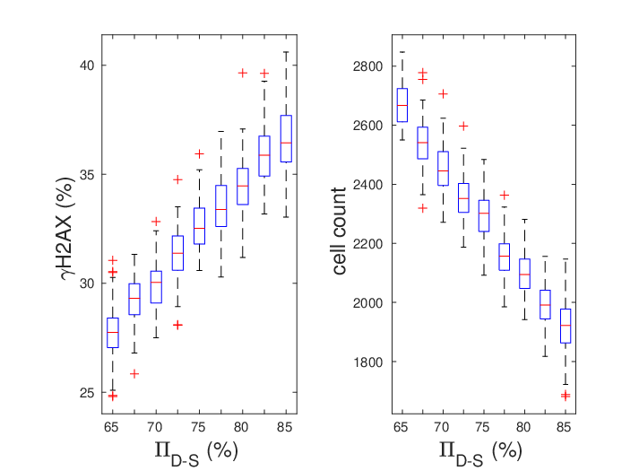
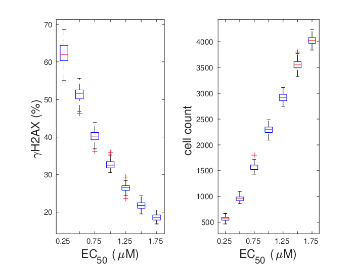
Steps 2 and 3: Post in silico simulations, the -measures are computed and plotted over all parameter values for each input parameter . Such plots are here shown for input parameters (Figure 11), (Figure 12) and (Figure 13).
The data samples produced in the in silico experiments are also represented using boxplots in these figures. The -measures and the boxplots demonstrate the effect that local perturbations of the input parameters have on both output responses and .
Figure 11 illustrates that increasing the probability that a cell enters the damaged S state increases the percentage of H2AX-positive cells and decreases the cell count, as is to be expected. Further, Figure 12 demonstrates that the model output is highly sensitive to perturbations of . Increasing results in a higher percentage of H2AX-positive cells and a lower cell count. Finally, Figure 13 shows that the regarded output responses are less sensitive to small perturbations of the Hill-exponent than to small perturbations of and .




6.3 Worked example: Latin Hypercube Analysis
Following steps 1, 2 and 3, as described in the quick guide in Section 5.3, Latin Hypercube Analysis is here performed in order to investigate how sensitive output responses are to global parameter perturbations.
We here investigate parameter values within parameter ranges that we consider to be ‘plausible’ post Robustness Analysis.
Step 1: For each input parameter, we decide to split the investigated parameter range into intervals. Why 100 you might ask? Well, in the original paper where we first introduced this model [9], the model took seven input parameters and thus . Accordingly, we tried using and intervals at first (following the suggestions discussed in Section 5) but neither of these options produced enough data samples to yield meaningful information in steps 2 and 3 below. Therefore, we decided to use instead, as this choice covered a larger range of the input parameter space whilst coming at a feasible computational cost. Now, we can use the built-in MATLAB function lhsdesign [17] to create combinations of input parameter values (represented by a point in input parameter space) that shall be used to produce the in silico data samples needed for Latin Hypercube Analysis.
Step 2: For each , median output responses ( and ) of in silico runs are computed. These are plotted in ’output-over-input’ scatterplots for each investigated input parameter in Figures 14, 15 and 16. From these figures we can make some qualitative remarks: Figure 14 indicates that the relationships between the input variable and the output responses and are, respectively, positively and negatively correlated. This agrees with the intuitive notion that if the probability that a cell enters the D-S state increases, so does the percentage of damaged cells () whilst the cell count () decreases as more cells will be susceptible to the drug and potentially die. The scatterplots in Figure 15 demonstrate that the input variable impacts the output responses more than do other investigated input parameters (within the regarded ranges). is negatively, linearly correlated with and positively, linearly correlated with . In Figure 16, however, there is no visually apparent correlation between the input parameter and the output.
Step 3: After making some qualitative remarks in Step 2, we now compute the Pearson Product Moment Correlation Coefficients between the various input-output pairs for a quantitative analyses. These correlation coefficients are listed in Table 3. To decide threshold values for correlation coefficient descriptors, we here compromise between threshold values suggested by other authors (listed in table 1) whilst taking into account that we are only regarding parameter values within ‘plausible’ ranges. With this as a guide, we here decide to refer to the linear input-output relationship as being ‘negligible’ for , where the obtained correlation coefficients are 0.05 and 0.12 for and respectively. We further say that for the linear input-output relationship is positively/negatively weak for and respectively. For , however, the linear input-output relationship is moderately negative for and strongly positive for . Clearly, we must be careful when choosing our value in the model, as this highly influences the model output!
| \diaghead(-3,2){\hskip 71.13188pt}{{\footnotesize\shortstack[l]{output}}}{{\footnotesize\shortstack[r]{input}}} | |||
|---|---|---|---|
| 0.19 | -0.59 | 0.05 | |
| -0.24 | 0.84 | 0.12 |


7 Conclusion
This review is intended as a gentle, introductory review to three uncertainty and sensitivity analyses methods, namely, Consistency Analysis, Robustness Analysis and Latin Hypercube Analysis. Information on how to implement these methods in MATLAB are available in the Appendix. Alternatively, all methods discussed in this review can be implemented using the R-based software package Spartan, developed by Alden et al. [1]. In fact, many of the proceedings and conventions used in this review follow those suggested by Alden et al. in order to allow the reader to, as easily as possible, use Spartan if desired. Scrutinising mathematical models using uncertainty and sensitivity analyses methods is an important part in model development. In many applications, knowledge about a model’s robustness is crucial [30]. In the context of quantitative pharmacology, for example, a mathematical model may be used to guide preclinical or, ultimately, clinical proceedings. In such cases, understanding how confident we can be with model results, and how sensitive a model is to parameter perturbations, is of the utmost importance.
Acknowledgements
SH was supported by the Medical Research Council [grant code MR/R017506/1] and Swansea University PhD Research Studentship. SS was supported by an STFC studentship under the DTP grant ST/N504464/1.
Appendix – MATLAB code snippets
Computing measure of stochastic superiority
We here list two different MATLAB functions that can be used in order to compute the point estimate of the A-measure of stochastic superiority in the original form, , and in the scaled form, . The function getA_measure_naive, listed below, uses direct implementations of Equations 9 and 11 to compute and return values for and , given two input vectors and . The function getA_measure uses the built-in MATLAB function ranksum to do the same.
Creating boxplots
The MATLAB function boxplot can be used to create boxplots. The input data in one column is represented by one box in the boxplot. For details regarding labeling and style alternatives, please see the MATLAB documentation [17].
Choosing Latin Hypercube Sampling points
A Latin Hypercube Sampling matrix can be created using the MATLAB function lhsdesign, which returns a matrix of size , where denotes the number of samples to be tested, and denotes the number of input parameters to investigate (and thus perturb).
Each row , in the created matrix (here denoted LHC_Matrix), corresponds to the th sampling point. Each element () corresponds to the parameter value of the th input parameter in sampling point , where each parameter ranges between 0 and 1. For different criteria on how to chose the specific parameter values within each sampled interval, please refer to the MATLAB documentation [17]. Sampling points can, for example, be chosen in a way that maximises the distance between sampling points in the -dimensional sampling space.
Qualitative and Quantitative Latin Hypercube Sampling Analysis
In order to qualitatively asses the correlation between an input parameter , and an output response , one can use the MATLAB function scatter. In the below listings, p and X are two data vectors.
Further, to quantify the linear correlation between and , the MATLAB function corrcoef can be used to compute correlation coefficients.
References
- [1] K. Alden, M. Read, J. Timmis, P. S. Andrews, H. Veiga-Fernandes, and M. Coles. Spartan: a comprehensive tool for understanding uncertainty in simulations of biological systems. PLoS Comput. Biol., 9(2):e1002916, 2013.
- [2] S.M. Blower and Hadi Dowlatabadi. Sensitivity and uncertainty analysis of complex models of disease transmission: An hiv model, as an example. International Statistical Review, 62, 08 1994.
- [3] E. O. Buzbas and N. A. Rosenberg. AABC: approximate approximate Bayesian computation for inference in population-genetic models. Theor Popul Biol, 99:31–42, Feb 2015.
- [4] A. Charzyńska, A. Nałęcz, M. Rybiński, and A. Gambin. Sensitivity analysis of mathematical models of signaling pathways. BioTechnologia., 93 (3):291–308, 2012.
- [5] S. Checkley, L. MacCallum, J. Yates, P. Jasper, H. Luo, J. Tolsma, and C. Bendtsen. Bridging the gap between in vitro and in vivo: Dose and schedule predictions for the ATR inhibitor AZD6738. Sci Rep, 5:13545, Aug 2015.
- [6] J. Cohen. The statistical power of abnormal-social psychological research: a review. J Abnorm Soc Psychol, 65:145–153, Sep 1962.
- [7] O. Cohen. Statistical Power Analysis for the Behavioral Sciences (Second Edition) . Lawrence Erlbaum Associates, 1988.
- [8] J. L. Gevertz and J. R. Wares. Developing a Minimally Structured Mathematical Model of Cancer Treatment with Oncolytic Viruses and Dendritic Cell Injections. Comput Math Methods Med, 2018:8760371, 2018.
- [9] S. Hamis, J. Yates, M.A.J Chaplain, and G.G. Powathil. Bridging in vitro and in vivo research via an agent-based modelling approach: predicting tumour responses to an atr-inhibiting drug. Preprint: bioRxiv, doi: 10.1101/841270.
- [10] R.L. Iman and J.C. Helton. Comparison of uncertainty and sensitivity analysis techniques for computer models. Report NUREGICR-3904, SAND 84-1461, Sandia National Laboratories, Albuquerque, New Mexico, 3 1985.
- [11] Timothy Krehbiel. Correlation coefficient rule of thumb. Decision Sciences Journal of Innovative Education, 2:97–100, 01 2004.
- [12] B. Lambert, A. L. MacLean, A. G. Fletcher, A. N. Combes, M. H. Little, and H. M. Byrne. Bayesian inference of agent-based models: a tool for studying kidney branching morphogenesis. J Math Biol, 76(7):1673–1697, 06 2018.
- [13] J. Liepe, P. Kirk, S. Filippi, T. Toni, C. P. Barnes, and M. P. Stumpf. A framework for parameter estimation and model selection from experimental data in systems biology using approximate Bayesian computation. Nat Protoc, 9(2):439–456, Feb 2014.
- [14] A. Ligmann-Zielinska, D. B. Kramer, K. Spence Cheruvelil, and P. A. Soranno. Using uncertainty and sensitivity analyses in socioecological agent-based models to improve their analytical performance and policy relevance. PLoS ONE, 9(10):e109779, 2014.
- [15] Shenglin Lin, Wei Li, Xiaochao Qian, Ping Ma, and Ming Yang. A Simulation Model Validation and Calibration Platform. pages 687–693, 12 2018.
- [16] G. Manache and C. Melching. Sensitivity of Latin Hypercube Sampling to sample size and distributional assumptions. 07 2007.
- [17] MATLAB. version 1.8.0_202 (R2019n). The MathWorks Inc., Natick, Massachusetts, 2019.
- [18] K. O. McGraw and S. P. Wong. A common language effect size statistic. Psychological Bulletin, 111(2):361–365, 1992.
- [19] M. D. McKay, R. J. Beckman, and W. J. Conover. Comparison of three methods for selecting values of input variables in the analysis of output from a computer code. Technometrics, 21(2):239–245, 1979.
- [20] Michael D. McKay. Latin hypercube sampling as a tool in uncertainty analysis of computer models. In Proceedings of the 24th Conference on Winter Simulation, WSC ’92, pages 557–564, New York, NY, USA, 1992. ACM.
- [21] M. M. Mukaka. Statistics corner: A guide to appropriate use of correlation coefficient in medical research. Malawi Med J, 24(3):69–71, Sep 2012.
- [22] A. Niida, T. Hasegawa, and S. Miyano. Sensitivity analysis of agent-based simulation utilizing massively parallel computation and interactive data visualization. PLoS ONE, 14(3):e0210678, 2019.
- [23] M. Read, P. S. Andrews, J. Timmis, and V. Kumar. Techniques for grounding agent-based simulations in the real domain: a case study in experimental autoimmune encephalomyelitis. Mathematical and Computer Modelling of Dynamical Systems, 18(1):67–86, 2012.
- [24] K. A. Rejniak and A. R. Anderson. Hybrid models of tumor growth. Wiley Interdiscip Rev Syst Biol Med, 3:115–125, 2011.
- [25] J. Ruscio and T. Mullen. Confidence Intervals for the Probability of Superiority Effect Size Measure and the Area Under a Receiver Operating Characteristic Curve. Multivariate Behavioral Research, 47(2):201–223, 2012.
- [26] Andrea Saltelli and Ricardo Bolado. An alternative way to compute fourier amplitude sensitivity test (fast). Comput. Stat. Data Anal., 26(4):445–460, February 1998.
- [27] P. Schober, C. Boer, and L. A. Schwarte. Correlation Coefficients: Appropriate Use and Interpretation. Anesth. Analg., 126(5):1763–1768, 05 2018.
- [28] Razi Sheikholeslami and Saman Razavi. Progressive latin hypercube sampling: An efficient approach for robust sampling-based analysis of environmental models. Environmental Modelling and Software, 93:109–126, 07 2017.
- [29] A. Vargha and H. D. Delaney. A Critique and Improvement of the CL Common Language Effect Size Statistics of McGraw and Wong. Journal of Educational and Behavioral Statistics, 25(2):101–132, 2000.
- [30] S. A. Visser, D. P. de Alwis, T. Kerbusch, J. A. Stone, and S. R. Allerheiligen. Implementation of quantitative and systems pharmacology in large pharma. CPT Pharmacometrics Syst Pharmacol, 3:e142, Oct 2014.
- [31] X. Y. Zhang, M. N. Trame, L. J. Lesko, and S. Schmidt. Sobol Sensitivity Analysis: A Tool to Guide the Development and Evaluation of Systems Pharmacology Models. CPT Pharmacometrics Syst Pharmacol, 4(2):69–79, 02 2015.