Bulk viscosity in neutron stars with hyperon cores

There are two well-known types of viscosities in a fluid. The shear viscosity $\eta$ comes from the momentum diffusion between fluid layers moving with different velocities. The bulk viscosity $\zeta$ appears due to non-equilibrium reactions in the compressing and decompressing fluid Landau and Lifshitz 2013.

Both these viscosities are important in numerous studies of neutron stars (NSs) Glampedakis and Gualtieri 2018, in particular, for damping of their r-mode oscillations Haskell 2015. The Rossby (or simply r-) modes are a subclass of the inertial oscillation modes, restoring force of which is the Coriolis force in a rotating star. The r-modes appear to be unstable to the gravitational wave emission due to the Chandrasekhar-Friedman-Schutz instability Chandrasekhar 1970; Friedman and Schutz 1978. It is damped by the shear and bulk viscosities at low and high temperatures, respectively. The domain in the $\nu,T$ plot ($\nu$ is the rotation frequency and $T$ is the internal temperature of the NS) where the star is unstable is called the r-mode instability window. It is highly unlikely to observe a NS with $\nu$ and $T$ within it. See the reviews Andersson and Kokkotas 2001; Haskell 2015.

However, one meets a paradox Haskell 2015: a lot of observed NSs in low-mass X-ray binaries (LMXBs) have their $\nu$ and $T$ in the unstable domain for NSs with the nucleonic ($npe\mu$) core composition. Namely, their typical temperatures are too hot to damp the instability by $\eta$ and too low to do it via $\zeta$. A lot of possible solutions to this paradox were proposed, mainly to introduce an additional damping mechanism. Some of them are reviewed in Haskell 2015. Here we focus on the option to modify the bulk viscosity $\zeta$ by the presence of hyperons in the NS core.

In a nucleonic core $\zeta$ is mainly provided by the modified Urca process, e.g. $n+n\to n+p+e+\tilde{\nu}_{e}$ and the inverse. In the most massive nucleonic NSs the direct Urca, $n\to p+e+\tilde{\nu}_{e}$ and the inverse, can operate. These non-equilibrium processes have the rates $\propto T^{6}\Delta\mu$ and $\propto T^{4}\Delta\mu$, respectively ($\Delta\mu$ is the chemical equilibrium distortions due to the fluid motions) Yakovlev et al. 2001; Haensel et al. 2000; Haensel et al. 2001. This means that at low temperatures these rates are strongly suppressed by a factor of $\sim(kT/\mu)^{4-6}$ ($\mu$ is a typical baryon chemical potential). The bulk viscosity due to these processes can damp the r-mode instability only at $T\sim 10^{9}-10^{10}\,$K, while NSs in LMXBs typically have $T\sim(0.3-1)\times 10^{8}\,$K. The suppression of the reaction rates due to nucleon pairing even worsens the problem Haensel et al. 2000; Haensel et al. 2001.

However, there are numerous models of the NS core equation of state (EoS) predicting the presence of hyperons (baryons with at least one strange quark) in deep layers of the core Haensel et al. 2007; Vidaña 2015. The most-widely used ones are the relativistic mean field (RMF) models due to their relative simplicity Glendenning 2000. The presence of hyperons dramatically changes the bulk viscosity. At low temperatures the main contribution to $\zeta$ comes from weak non-leptonic processes, e.g., $\Sigma^{-}+p\leftrightarrow n+n$ or $\Lambda+p\leftrightarrow n+p$. At $T<10^{9}\,$K their typical rate $\propto T^{2}\Delta\mu$ is much larger than the Urca process rates. There were numerous calculations of the reaction rates of these processes and the corresponding bulk viscosity Lindblom and Owen 2002; Haensel et al. 2002; van Dalen and Dieperink 2004; Nayyar and Owen 2006; Gusakov and Kantor 2008 in both normal and paired matter. Existing calculations of the r-mode instability windows for hyperonic NSs Lindblom and Owen 2002; Reisenegger and Bonačić 2003; Nayyar and Owen 2006 yield that the hyperonic enhancement of $\zeta$ is generally not enough to solve the r-mode paradox (except, maybe, for the most massive stars $\sim 2\,$M_⊙, central regions of which may be free of baryon pairing). In the recent reviews Haskell 2015; Vidaña 2015 it is argued that the hyperonic bulk viscosity is unable to close the instability window for the observed NSs. However, previous calculations of the instability window for hyperonic NSs should be revisited. First, they used the $\Sigma^{-}\Lambda$ hyperonic composition of the NS core. Various modern EoS models Gusakov et al. 2014a; Raduta et al. 2018; Negreiros et al. 2018, in particular those, calibrated to the up-to-date hypernuclear data Fortin et al. 2017; Providência et al. 2019 predict that $\Lambda$ and $\Xi^{-}$ are likely the first hyperons that appear with growing density ($\Sigma^{-}$-hyperons either appear at higher densities or do not appear at all in NSs). Second, calculations of Lindblom and Owen 2002; Reisenegger and Bonačić 2003; Nayyar and Owen 2006 employed reaction rates for non-leptonic weak processes derived using the contact exchange by the $W$ boson of two baryon currents. Still, it is well-known (see, e.g., Ref. Gal et al. 2016), that the most effective channel for a weak inelastic collision between a hyperon and another baryon is the meson (e.g $\pi$-meson) exchange. However, this channel was analyzed only once in Ref. van Dalen and Dieperink 2004 to calculate $\zeta$ in the NS hyperonic core. To the best of our knowledge, the results of Ref. van Dalen and Dieperink 2004 have never been used to compute the r-mode instability window.

In the present work we revisit the bulk viscosity in a non-superfluid hyperonic NS core. We consider RMF EoS models (Sec. II), for which the $\Lambda$ and $\Xi^{-}$ hyperons appear first ($\Sigma^{-}$ hyperons are also present in some of our EoSs, but we focus on the $\Lambda\Xi^{-}$ composition for simplicity). We derive relations between $\zeta$ and the rates of the weak non-leptonic processes for an arbitrary EoS (Sec. III). Then, adopting the one meson exchange weak interaction model, we calculate the rates for all weak non-leptonic processes operating in the $npe\mu\Lambda\Xi^{-}$ matter and responsible for the bulk viscosity (Sec. IV). Simple analytic approximations are proposed for $\zeta$ and the reaction rates. We continue by applying our results to calculate the r-mode instability windows for hyperonic NSs (Sec. V). Our results indicate that the hyperonic solution to the r-mode paradox is likely more viable than it was thought before. Conclusions and some discussion are given in Sec. VI.

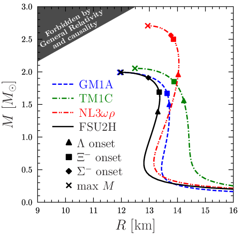
Four RMF models for the core EoS are employed in this work: GM1A and TM1C from Ref. Gusakov et al. 2014a, NL3$\omega\rho$ from Ref. Horowitz and Piekarewicz 2001, and FSU2H from Ref. Providência et al. 2019. The two last EoSs are calibrated to the up-to-date (hyper)nuclear data following the approach presented in Ref. Fortin et al. 2017, the former two are not. For the FSU2H in particular we use a $\Sigma^{-}$ potential in the symmetric nuclear matter of $40$ MeV so that $\Sigma^{-}$ appear at large enough densities and masses: $M>1.9$ M_⊙ (see also the discussion in Ref. Providência et al. 2019). In each case, the crust EoS is calculated consistently to the core one, similarly as it was done in Providência et al. 2019; Fortin et al. 2016.

The main astrophysical parameters for the four models are listed in Table 1. Fig. 2 shows the pressure $P$ as a function of the density and Fig. 2 the associated relations between the mass $M$ and the radius $R$ of NSs as obtained when solving the Tolman-Oppenheimer-Volkov equations (e.g. Lindblom 1992) for these EoSs. One can see that for the models considered here $\Lambda$ appears first, $\Xi^{-}$ comes after, and then other hyperon species emerge at rather high densities and NS masses. This allows us to diminish the number of reactions responsible for the bulk viscosity we have to consider. In particular, within this EoS set we can limit ourselves to the properties of $npe\mu\Lambda\Xi^{-}$ composition up to $M\leqslant 1.9$ M_⊙.

All models we consider are consistent with the existence of the most massive NSs with a precisely measured mass: PSR J$1614-2230$ Demorest et al. 2010; Arzoumanian et al. 2018 and PSR J$0348+0432$ Antoniadis et al. 2013 with NL3$\omega\rho$ giving the largest maximum mass of all models: $\sim 2.7$ M_⊙ compared to $\sim 2$ M_⊙ for the three other paramterizations. However only NL3$\omega\rho$ and FSU2H have values of the symmetry energy and its slope consistent with modern experimental constraints (see the discussion in e.g. Fortin et al. 2016; Oertel et al. 2017). Of all models, FSU2H gives the lowest radii $R\sim 13$ km of NSs with the canonical mass $1.4$ M_⊙. Note that for the hyperonic FSU2H EoS hyperons are present in NSs with a mass larger than $1.38$ M_⊙.

Figure 3 shows that the four models have significantly different composition, and we thus expect them to give different properties for the bulk viscosity.

With the method presented in Ref. Gusakov et al. 2014a we have calculated the Landau effective masses $m^{*}_{\text{L}j}$ and Landau parameters $F_{0}^{jk}$ and $F_{1}^{jk}$ ($j$ and $k$ for all baryon species presented for a given EoS). The quantities $m^{*}_{\text{L}j}$ and $F_{0}^{jk}$ are necessary for bulk viscosity calculations. We would like to stress that baryon Fermi velocities $v_{\text{F}j}=p_{\text{F}j}/m^{*}_{\text{L}j}$ are close to the unity (i.e. to the speed of light) in a wide range of densities for all EoSs considered, see Figure 4 for details. In other words, baryons (particularly nucleons) are essentially relativistic even at densities typical of a moderately heavy NS, $M\sim 1.5-1.9$ M_⊙. Thus one has to work in the relativistic framework like, e.g., in Refs. Lindblom and Owen 2002; van Dalen and Dieperink 2004; Nayyar and Owen 2006, rather than in the nonrelativistic one (as, e.g., in Ref. Haensel et al. 2002), while calculating reaction rates for the bulk viscosity.

Bulk viscosity is generated due to non-equilibrium reactions. In the case of the nucleon $npe\mu$ matter the main reactions are the Urca processes Haensel et al. 2000; Haensel et al. 2001. When the hyperons appear, the non-leptonic weak processes become the main source for the bulk viscosity (see, e.g., Lindblom and Owen 2002; Haensel et al. 2002), since they are much more intensive at typical NS temperatures. There are a lot of such processes. If $\Lambda$ is the only hyperon species in the matter, the reactions are

The appearance of any additional hyperon species increases the number of the relevant processes significantly. Notice also that we consider only those reactions which change the strangeness by unity, $|\Delta S|=1$.

Non-equilibrium rates of these processes, $\Delta\Gamma_{\alpha}$, $\alpha=(a)$, $(b)$, $(c)$, $(d)$, $(e)$, depend on the chemical equilibrium perturbations $\Delta\mu_{\alpha}$, where, e.g., $\Delta\mu_{(a)}=\mu_{n}-\mu_{\Lambda}$, $\Delta\mu_{(e)}=\mu_{\Lambda}+\mu_{n}-\mu_{\Xi^{-}}-\mu_{p}$, etc. In the subthermal regime, $\Delta\mu_{\alpha}\ll kT$ ($k$ is the Boltzmann constant), the reaction rates can be written as

In what followsthe quantities $\lambda_{\alpha}$ and $\Delta\Gamma_{\alpha}$ will be both referred to as “the reaction rates”

There are also strong hyperon reactions in the NS core. In the absence of pairing they are $\sim 14-16$ orders of magnitude faster than the weak non-leptonic ones. For NS oscillations of interest, with frequency $\sim 10^{2}-10^{4}$ Hz, the core matter can be considered as equilibrated with respect to them. In spite of that, strong processes are also important for the bulk viscosity calculation (see below).

There are no strong hyperon reactions in the $npe\mu\Lambda$ matter. If we add $\Xi^{-}$, the only strong process is

Linear combinations of these reactions are also possible. The complete set of reactions for the full baryon octet can be found in appendix C of Gusakov et al. 2014a.

We follow Ref. Gusakov and Kantor 2008 in describing the recipe to derive the bulk viscosity in a form convenient for studying dissipation during NS oscillations.

Density variations $\delta n_{j}$ are linearly dependent, because they are related by the electric neutrality condition

($e_{j}$ is the electric charge of the particle species $j$) and equilibrium conditions with respect to strong reactions [e.g., the reactions in Eqs (3)]:

etc., supplemented with Eq. (4) for $\delta\mu_{j}$. Therefore, for any number of particle species, only four of density perturbations $\delta n_{j}$ are independent.

Another important consequence of Eqs. (8) is that for all non-leptonic weak processes we have

This is, in particular, true for reactions that are listed in Eqs. (1).

The most convenient choice of four independent thermodynamic parameters is: the baryon number density $n_{b}$ (conserved in all reactions), the electron and muon fractions $y_{e,\mu}=n_{e,\mu}/n_{b}$ (conserved since we restrict ourselves to non-leptonic reactions), and the strangeness fraction $y_{s}=\sum_{j}S_{j}n_{j}/n_{b}$, where $S_{j}$ is the strangeness of the species $j$. Only weak processes contribute to the strangeness production since it is conserved in strong reactions. As we consider weak non-leptonic reactions with $\Delta S=1$ only, the total strangeness production rate $\Delta\Gamma_{S}$ is just the sum of all partial rates $\Delta\Gamma_{\alpha}$. Employing Eq. (9) and bearing in mind that $S_{j}<0$, we have

where $\lambda$ is the total reaction rate of all non-leptonic weak processes.

The continuity Eqs. (6) lead to

Considering all thermodynamic quantities as functions of $n_{b}$ and $y_{e,\mu,s}$ and accounting for Eq. (11b), we get

with $\partial\Delta\mu/\partial X=\partial\mu_{n}/\partial X-\partial\mu_{\Lambda}/\partial X$ stemming from Eq. (9). Near-equilibrium derivatives with respect to $n_{b}$ and $y_{s}$ can be derived from Eqs. (4), (7), and (8). The quantity $\delta P_{\text{eq}}$ should be calculated with Eq. (12a) assuming that all reactions are switched off, i.e. $\delta y_{s}=0$ as well as $\delta y_{e}=0$ and $\delta y_{\mu}=0$.

Combining Eqs. (5), (11), and (12) we have (cf. the formulas (22) in Gusakov and Kantor 2008 and (17) in Haensel et al. 2002)

where

Eq. (13) shows a well-known feature of the hyperon bulk viscosity Lindblom and Owen 2002; Haensel et al. 2002; van Dalen and Dieperink 2004; Nayyar and Owen 2006; Haskell 2015: it has a maximum with respect to the rate of non-equilibrium processes $\lambda$. Consequently, it has a maximum with respect to temperature since $\lambda$ grows with it. Apart from $\lambda$ the bulk viscosity depends on two parameters i.e., $\zeta_{\mathrm{max}}$ which is the maximum possible bulk viscosity, and $\lambda_{\mathrm{max}}$ which is the optimal total reaction rate for a given oscillation frequency $\omega$. They are determined by the thermodynamic properties of the EoS only, and not by reactions operating in the matter.

Figure 5 shows $\zeta_{\mathrm{max}}$ and $\lambda_{\mathrm{max}}$ as functions of energy density $\rho$. All the curves start from zero at the points of $\Lambda$ onset. The appearance of a new hyperon causes a rapid increment of the optimum rate $\lambda_{\mathrm{max}}$, however, without discontinuity. The maximum viscosity $\zeta_{\mathrm{max}}$ increases when each of cascade hyperons appears, and decreases when $\Sigma^{-}$ appears. But the main feature of plots in Figure 5 is that both $\zeta_{\mathrm{max}}$ and $\lambda_{\mathrm{max}}$ are strongly sensitive to the EoS model. However, at not too high densities, $\rho\lesssim 3\rho_{0}$, for all EoSs considered $\lambda_{\mathrm{max}}(\rho)$ has similar behaviour and values.

When only $\Lambda$ and $\Xi^{-}$ hyperons are present in the core, the averaged behavior of the curves in Fig. 5 is roughly reproduced by formula

where $\omega_{4}=\omega/(10^{4}\,\text{s}^{-1})$ and $\rho_{\Lambda}$ is the density of $\Lambda$ hyperon onset (see Table 1). The fitting parameters are $\zeta_{0}=6.5\times 10^{30}\,$g cm${}^{-1}\,$s^-1, $\lambda_{0}=8.0\times 10^{45}\,$erg${}^{-1}\,$cm${}^{-3}\,$s^-1, $t=0.34$, and $s=1.0$ for $\zeta_{\mathrm{max}}$ (maximum error $\sim 60\%$) and $s=1.5$ for $\lambda_{\mathrm{max}}$ (maximum error $\sim 20\%$) respectively. We emphasize that the power $t$ describing the behavior at $\rho\to\rho_{\Lambda}$ is the same for both these quantities. The thicker grey curves in Fig. 5 show how this fit works, and the thinner ones visualize 60% and 20% uncertainties for $\zeta_{\mathrm{max}}$ and $\lambda_{\mathrm{max}}$, correspondingly. Of course, Eq. (15) does not reproduce kinks at the $\Xi^{-}$ onset points and it does not describe behavior of the curves after appearance of $\Sigma^{-}$ or $\Xi^{0}$ hyperon. However, the four EoSs we use here are significantly different, and we can hope that, for the $npe\mu\Lambda\Xi^{-}$ matter, any other RMF model would give $\zeta_{\mathrm{max}}$ and $\lambda_{\mathrm{max}}$ within the range of uncertainties predicted by our fit (15).

When plotting r-mode instability windows, the averaged fit for $\lambda_{\mathrm{max}}^{\text{appr}}$ appears to be rather accurate, but the fit for $\zeta_{\mathrm{max}}^{\text{appr}}$, without additional corrections, fails to reproduce the r-mode instability window for some specific EoS. See the end of Sec. V and the caption to Fig. 13 for a description of how one should use Eq. (15) to solve this problem.

Now, the question is how close the “real” reaction rate of weak non-leptonic reactions $\lambda$ can be to the optimum rate.

References

- Landau and Lifshitz (2013) L. Landau and E. Lifshitz, Fluid Mechanics, V., 6 (Elsevier Science, Oxford, 2013), ISBN 9781483140506.
- Glampedakis and Gualtieri (2018) K. Glampedakis and L. Gualtieri, in Astrophysics and Space Science Library, edited by L. Rezzolla, P. Pizzochero, D. I. Jones, N. Rea, and I. Vidaña (2018), vol. 457 of Astrophysics and Space Science Library, p. 673, eprint 1709.07049.
- Haskell (2015) B. Haskell, International Journal of Modern Physics E 24, 1541007 (2015), eprint 1509.04370.
- Chandrasekhar (1970) S. Chandrasekhar, Phys. Rev. Lett. 24, 611 (1970).
- Friedman and Schutz (1978) J. L. Friedman and B. F. Schutz, Astrophys. J. 222, 281 (1978).
- Andersson and Kokkotas (2001) N. Andersson and K. D. Kokkotas, International Journal of Modern Physics D 10, 381 (2001), eprint gr-qc/0010102.
- Yakovlev et al. (2001) D. G. Yakovlev, A. D. Kaminker, O. Y. Gnedin, and P. Haensel, Phys. Rep. 354, 1 (2001), eprint astro-ph/0012122.
- Haensel et al. (2000) P. Haensel, K. P. Levenfish, and D. G. Yakovlev, Astron. Astrophys. 357, 1157 (2000), eprint astro-ph/0004183.
- Haensel et al. (2001) P. Haensel, K. P. Levenfish, and D. G. Yakovlev, Astron. Astrophys. 372, 130 (2001), eprint astro-ph/0103290.
- Haensel et al. (2007) P. Haensel, A. Y. Potekhin, and D. G. Yakovlev, Neutron Stars. 1. Equation of State and Structure (Springer, New York, 2007).
- Vidaña (2015) I. Vidaña, in American Institute of Physics Conference Series (2015), vol. 1645 of American Institute of Physics Conference Series, pp. 79–85.
- Glendenning (2000) N. K. Glendenning, Compact stars : nuclear physics, particle physics, and general relativity, Astronomy and astrophysics library (Springer, New York, 2000).
- Lindblom and Owen (2002) L. Lindblom and B. J. Owen, Phys. Rev. D 65, 063006 (2002), eprint astro-ph/0110558.
- Haensel et al. (2002) P. Haensel, K. P. Levenfish, and D. G. Yakovlev, Astron. Astrophys. 381, 1080 (2002), eprint astro-ph/0110575.
- van Dalen and Dieperink (2004) E. N. van Dalen and A. E. Dieperink, Phys. Rev. C 69, 025802 (2004), eprint nucl-th/0311103.
- Nayyar and Owen (2006) M. Nayyar and B. J. Owen, Phys. Rev. D 73, 084001 (2006), eprint astro-ph/0512041.
- Gusakov and Kantor (2008) M. E. Gusakov and E. M. Kantor, Phys. Rev. D 78, 083006 (2008), eprint 0806.4914.
- Reisenegger and Bonačić (2003) A. Reisenegger and A. Bonačić, Phys. Rev. Lett. 91, 201103 (2003), eprint astro-ph/0303375.
- Gusakov et al. (2014a) M. E. Gusakov, P. Haensel, and E. M. Kantor, Mon. Not. R. Astron. Soc. 439, 318 (2014a), eprint 1401.2827.
- Raduta et al. (2018) A. R. Raduta, A. Sedrakian, and F. Weber, Mon. Not. R. Astron. Soc. 475, 4347 (2018), eprint 1712.00584.
- Negreiros et al. (2018) R. Negreiros, L. Tolos, M. Centelles, A. Ramos, and V. Dexheimer, Astrophys. J. 863, 104 (2018), eprint 1804.00334.
- Fortin et al. (2017) M. Fortin, S. S. Avancini, C. Providência, and I. Vidaña, Phys. Rev. C 95, 065803 (2017).
- Providência et al. (2019) C. Providência, M. Fortin, H. Pais, and A. Rabhi, Frontiers in Astronomy and Space Sciences 6, 13 (2019), eprint 1811.00786.
- Gal et al. (2016) A. Gal, E. V. Hungerford, and D. J. Millener, Reviews of Modern Physics 88, 035004 (2016), eprint 1605.00557.
- Horowitz and Piekarewicz (2001) C. J. Horowitz and J. Piekarewicz, Phys. Rev. Lett. 86, 5647 (2001), eprint astro-ph/0010227.
- Fortin et al. (2016) M. Fortin, C. Providência, A. R. Raduta, F. Gulminelli, J. L. Zdunik, P. Haensel, and M. Bejger, Phys. Rev. C 94, 035804 (2016), eprint 1604.01944.
- Lindblom (1992) L. Lindblom, Astrophys. J. 398, 569 (1992).
- Demorest et al. (2010) P. B. Demorest, T. Pennucci, S. M. Ransom, M. S. E. Roberts, and J. W. T. Hessels, Nature (London) 467, 1081 (2010), eprint 1010.5788.
- Arzoumanian et al. (2018) Z. Arzoumanian, A. Brazier, S. Burke-Spolaor, S. Chamberlin, S. Chatterjee, B. Christy, J. M. Cordes, N. J. Cornish, F. Crawford, H. Thankful Cromartie, et al., Astrophys. J. Suppl. Ser. 235, 37 (2018), eprint 1801.01837.
- Antoniadis et al. (2013) J. Antoniadis, P. C. C. Freire, N. Wex, T. M. Tauris, R. S. Lynch, M. H. van Kerkwijk, M. Kramer, C. Bassa, V. S. Dhillon, T. Driebe, et al., Science 340, 448 (2013), eprint 1304.6875.
- Oertel et al. (2017) M. Oertel, M. Hempel, T. Klähn, and S. Typel, Reviews of Modern Physics 89, 015007 (2017), eprint 1610.03361.
- Jones (2001) P. B. Jones, Phys. Rev. D 64, 084003 (2001).
- Gusakov et al. (2005) M. E. Gusakov, D. G. Yakovlev, and O. Y. Gnedin, Mon. Not. R. Astron. Soc. 361, 1415 (2005), eprint astro-ph/0502583.
- Shapiro and Teukolsky (1983) S. L. Shapiro and S. A. Teukolsky, Black holes, white dwarfs, and neutron stars : the physics of compact objects (A Wiley-Interscience Publication, New York, 1983).
- Parreño et al. (1997) A. Parreño, A. Ramos, and C. Bennhold, Phys. Rev. C 56, 339 (1997), eprint nucl-th/9611030.
- Itonaga and Motoba (2010) K. Itonaga and T. Motoba, Progress of Theoretical Physics Supplement 185, 252 (2010).
- Bauer et al. (2017) E. Bauer, G. Garbarino, and C. A. Rodríguez Peña, Physics Letters B 766, 144 (2017), eprint 1701.03957.
- Parreño et al. (1999) A. Parreño, A. Ramos, N. G. Kelkar, and C. Bennhold, Phys. Rev. C 59, 2122 (1999), eprint nucl-th/9810020.
- Pérez-Obiol et al. (2013) A. Pérez-Obiol, D. R. Entem, B. Juliá-Díaz, and A. Parreño, Phys. Rev. C 87, 044614 (2013), eprint 1302.6955.
- Parreño et al. (2002) A. Parreño, A. Ramos, and C. Bennhold, Phys. Rev. C 65, 015205 (2002), eprint nucl-th/0106054.
- Bauer et al. (2015) E. Bauer, G. Garbarino, and C. A. Rodríguez Peña, Phys. Rev. C 92, 014301 (2015), eprint 1503.06125.
- Grotz and Klapdor (1990) K. Grotz and H. V. Klapdor, The weak interaction in nuclear, particle and astrophysics. (CRC Press, Boca Raton, 1990).
- Okun (2014) L. B. Okun, Leptons and Quarks (WORLD SCIENTIFIC, New York, 2014).
- Rijken et al. (1999) T. A. Rijken, V. G. J. Stoks, and Y. Yamamoto, Phys. Rev. C 59, 21 (1999), eprint nucl-th/9807082.
- Friman and Maxwell (1979) B. L. Friman and O. V. Maxwell, Astrophys. J. 232, 541 (1979).
- Maxwell (1987) O. V. Maxwell, Astrophys. J. 316, 691 (1987).
- Akmal et al. (1998) A. Akmal, V. R. Pandharipande, and D. G. Ravenhall, Phys. Rev. C 58, 1804 (1998), eprint nucl-th/9804027.
- Potekhin et al. (2013) A. Y. Potekhin, A. F. Fantina, N. Chamel, J. M. Pearson, and S. Goriely, Astron. Astrophys. 560, A48 (2013), eprint 1310.0049.
- Kolomeitsev et al. (2003) E. E. Kolomeitsev, N. Kaiser, and W. Weise, Phys. Rev. Lett. 90, 092501 (2003), eprint nucl-th/0207090.
- Kolomeitsev (2018) E. E. Kolomeitsev, private communication (2018).
- Migdal et al. (1990) A. B. Migdal, E. E. Saperstein, M. A. Troitsky, and D. N. Voskresensky, Phys. Rep. 192, 179 (1990).
- Page et al. (2015) D. Page, J. M. Lattimer, M. Prakash, and A. W. Steiner, in Novel Superfluids, vol. 2,, edited by K. H. Bennemann and J. B. Ketterson (International Series of Monographs on Physics, vol. 157, 505, Oxford University Press, Oxford, 2015), vol. 157, pp. 505–579.
- Sedrakian and Clark (2019) A. Sedrakian and J. W. Clark, European Physical Journal A 55, 167 (2019), eprint 1802.00017.
- Takatsuka et al. (2006) T. Takatsuka, S. Nishizaki, Y. Yamamoto, and R. Tamagaki, Progress of Theoretical Physics 115, 355 (2006), eprint nucl-th/0601043.
- Takahashi et al. (2001) H. Takahashi, J. K. Ahn, H. Akikawa, S. Aoki, K. Arai, S. Y. Bahk, K. M. Baik, B. Bassalleck, J. H. Chung, M. S. Chung, et al., Phys. Rev. Lett. 87, 212502 (2001).
- Oppenheimer and Volkoff (1939) J. R. Oppenheimer and G. M. Volkoff, Physical Review 55, 374 (1939).
- Tolman (1939) R. C. Tolman, Physical Review 55, 364 (1939).
- Lindblom et al. (1998) L. Lindblom, B. J. Owen, and S. M. Morsink, Phys. Rev. Lett. 80, 4843 (1998), eprint gr-qc/9803053.
- Schmitt and Shternin (2018) A. Schmitt and P. Shternin, in The Physics and Astrophysics of Neutron Stars, edited by L. Rezzolla, P. Pizzochero, D. I. Jones, N. Rea, and I. Vidaña (2018), vol. 457 of Astrophysics and Space Science Library, p. 455, eprint 1711.06520.
- Shternin (2018) P. S. Shternin, Phys. Rev. D 98, 063015 (2018), eprint 1805.06000.
- Gusakov et al. (2014b) M. E. Gusakov, A. I. Chugunov, and E. M. Kantor, Phys. Rev. D 90, 063001 (2014b), eprint 1305.3825.
- Allen et al. (2018) J. L. Allen, J. Homan, D. Chakrabarty, and M. Nowak, Astrophys. J. 854, 58 (2018).
- Bilous et al. (2018) A. V. Bilous, A. L. Watts, D. K. Galloway, and J. J. M. in ’t Zand, Astrophys. J. 862, L4 (2018), eprint 1805.10065.
- Chatterjee and Bandyopadhyay (2006) D. Chatterjee and D. Bandyopadhyay, Phys. Rev. D 74, 023003 (2006), eprint astro-ph/0602538.
- Voskresensky (2001) D. N. Voskresensky, in Physics of Neutron Star Interiors, edited by D. Blaschke, N. K. Glendenning, and A. Sedrakian (Springer, Berlin, 2001), vol. 578 of Lecture Notes in Physics, p. 467.
- Kantor and Gusakov (2009) E. M. Kantor and M. E. Gusakov, Phys. Rev. D 79, 043004 (2009), eprint 0901.4108.
- Lee and Yoshida (2003) U. Lee and S. Yoshida, Astrophys. J. 586, 403 (2003), eprint astro-ph/0211580.
- Haskell and Andersson (2010) B. Haskell and N. Andersson, Mon. Not. R. Astron. Soc. 408, 1897 (2010), eprint 1003.5849.
- Kantor and Gusakov (2017) E. M. Kantor and M. E. Gusakov, Mon. Not. R. Astron. Soc. 469, 3928 (2017), eprint 1705.06027.
- Dommes et al. (2019) V. A. Dommes, E. M. Kantor, and M. E. Gusakov, Mon. Not. R. Astron. Soc. 482, 2573 (2019), eprint 1810.08005.