Pattern of lensed chirp gravitational wave signal and its implication on the mass and position of lens

Dongze Sun, Xilong Fan Alternate Affiliation: Hongyi Honor School, Wuhan University Alternate Affiliation: School of Physics and Technology, Wuhan University

Abstract

We prose a new measurement strategy of the estimation the lens mass, as well as the actual amplification, of the lens through the modulation patten of lensed gravitational wave signals alone. This can be done by measuring the frequency and amplitude ratio of peaks and valleys of the modulation pattern of CBC signals , known as “beat”, which is a time domain phenomenon of strong lens effect.

I. INTRODUCTION

The detection of gravitational waves (GWs) by LIGO/Virgo collaborations LIGO/Virgo collaborations 2016 open the new era of the GW astronomy and the multi-messenger astronomy. If gravitational waves pass through a massive body in the process of propagation, they can be gravitationally lensed P. Schneider, J. Ehlers, and E. E. Falco 1992. The effects of lensed the tensor wave nature of GW (e.g. rotation of the polarization plane of GW Hou et al. 2019a ) is negligible for most lensed systerms. Only the amplification effect (e.g. Takahashi & Nakamura 2003) of the lens is the investigated in most literature.

In the context of 3rd generation interferometric ground detectors - the Eistein Telescope in particular - quite recent series of papers explored the perspectives of observing gravitationally lensed coalescing double compact objects by the ET for the SIS lens model (Piórkowska, Biesiada & Zhu 2013; Biesiada et al. 2014; Ding, Biesiada & Zhu 2015) and more realistic lens model Li et al. 2018, respectively. Rates of lensed GW in adLIGO were reassessed by Ng et al. 2018, Yang et al. 2019.

Under the geometrical optics approximation, the lensing effects for parameters estimation for individual inspiral signal and the population of black hole mergers were addressed in Cao et al. 2014 and Dai et al. 2017 for ground-based detectors, respectively.

Nakamura 1998 has first taken correct account of the diffraction effect in GW lensing and demonstrated that when the lens is much lighter than $\sim 10^{2}\;M_{\odot}$ , the diffraction is so effective that the geometric optics cannot be used anymore. This subject has been advanced in the papers by Takahashi & Nakamura 2003,Takahashi 2016 and K. Liao, M. Biesiada, and X.-L. Fan 2019.

Given the fact of laking sky localization ability of GW detectors, previous studies of applications of the lensed gravitational waves as a astrophysical tool focus on the multi-messenger approach, namely people need to identify the host galaxy by their em counterpart to get the information of source redshift and the lens potential. The GW speed Fan et al. 2017; Baker & Trodden 2017; Collett & Bacon 2017, the Hubble constant Liao et al. 2017 cosmic curvature Li et al. 2019 and dark matter substructure Li et al. 2018 have been studied with the information of the time-delay from GW and redshift and location from EM signals of a strong lens system. The multi-messenger approach could only apply for the bns signal, while the major detection of GW should be BBH.

Recently, with the beat pattern of lensed GW alone, Hou et al. 2019b used matched filter strategy to determine the lens mass and the actual amplification of the point mass and SIS model under the geometrical optics approximation assuming known template for the lensed GWs.

In this paper we propose a waveform independent methord to measure lens parameters and the actual amplification by the “beat” pattern of the strong lensed gravitational wave. This paper is organized as follows: In section II we give the formulation of the lensing effect of GW, and introduce the characteristics of patterns in the lensed signals. In section III we provide the condition under which patterns can show up, and we discuss the relationship between the characters of patterns and parameters of both source and lens. Then we present a new approach to detect the information of gravitational lens and GW source. In section IV we choose the CBC waveform and point-mass lens model as an example, to illuminate the characteristics of patterns we have discussed, and to show how our method works. And we give a summary in section V.

II. LENSING EFFECT OF GW

In a gravitational lens system, we denote the distances between the source and lens, lens and observer, source and observer as $D_{LS}$ , $D_{L}$ and $D_{S}$ respectively, 2 dimensional vector $\bm{\eta}$ denotes the distance of the source from the attachment of lens and observer, and $\bm{\xi}$ is a position vector on lens plane.

Following Takahashi & Nakamura 2003, for a monochromatic wave with frequency $f$ , the effect of gravitational lens can be described by amplification factor $F(f)$ defined as:

F_{+,\times}(f)=\frac{\tilde{h}_{+,\times}^{L}(f)}{\tilde{h}_{+,\times}(f)}.

(1)

The frequency and polarization of the signal is not influenced by the lens and only the amplitude is remodulated.

The amplification factor is given by:

F(f,y)=\frac{D_{S}\xi_{0}^{2}}{D_{L}D_{LS}}\frac{f}{i}\int\mathrm{d}^{2}\bm{x}\exp[2\pi ift_{d}(\bm{x},\bm{y})],

(2)

where $\bm{x}=\bm{\xi}/\xi_{0},\bm{y}=\bm{\eta}D_{L}/\xi_{0}D_{S}$ , and $\xi_{0}$ is an arbitrary normalization constant.

For the ground detectors, the detected signal in time domain is then

h^{L}(t)=[A^{+}h^{L}_{+}(t)+A^{\times}h^{L}_{\times}(t)],

(3)

where $A^{+}$ and $A^{\times}$ are antenna patten of the detector, and $h^{L}_{+,\times}(t)$ is the lensed GW signal in time domain. Hereafter we assume the antenna patten is a constant.

II.1. The beat pattern

When the wavelength of source signal is much larger than the Schwarzschild radius of the gravitational lens, there is no pattern but the amplification of the signal. While the wavelength is comparable with the Schwarzschild radius of lens, the patterns show up, and exist when wavelength is small enough to enter the realm of geometric optics. Here we drive the exact condition for the patterns to show up for the strong lensed case.

To analyze the pattern on the lensed signal, we compute the envelope of the signal using Hilbert transform:

A^{L}(t)=\left|\frac{1}{\pi}\int\frac{h^{L}(\tau)}{t-\tau}\mathrm{d}\tau\right|,

(4)

where $h^{L}(\tau)$ is the lensed GW signal. The position of peaks and valleys of the envelope are related to the lens mass $M_{L}$ and position $y$ . Note that for a typical lens (such as SIS and point mass model), the amplification factor is a function of the product of lens mass $M_{L}$ and the GW frequency $f$ : $w=M_{L}f$ , so the lensed GW signal $\tilde{h}^{L}(f)$ in frequency domain can be written as:

\tilde{h}^{L}(f)=F(w)\tilde{h}(f),

(5)

So when the frequency changes slowly (e.g. $\dot{f}\ll f^{2}$ ), a necessary condition for peaks of the envelope in this case is:

\frac{\mathrm{d}F(w)}{\mathrm{d}w}\bigg|_{f=f_{p}}=0,

(6)

where $f_{p}$ is the frequency of peaks of the envelope. So we have $f_{p}\propto 1/M_{L}$ in this case. The condition $\dot{f}\ll f^{2}$ is valid for all lensed CBCs in the wave region $\lambda\sim R_{s}$ , and even valid for part of optical region, so we can obtain the proportional coefficient in geometric optical region.

F(f)=\sum_{j}\mu_{j}^{1/2}e^{i2\pi ft_{dj}-i\pi n_{j}},

(7)

meaning that discrete images interfere with each other, where $\mu_{j}$ is the magnification of the $j$ th image, $t_{dj}=t_{d}(\bm{x_{j}},\bm{y})$ , and $n_{j}=0,1/2,1$ when $\bm{x_{j}}$ is a minimum, saddle, and maximum point respectively of $t_{d}(\bm{x},\bm{y})$ .

Suppose there are only two images, e.g., in the case of point-mass model and SIS model, if $t_{0}$ is the time of $n$ th peak $f_{p}(n)$ and $t_{0}+\Delta t$ is the time of $(n+1)$ th peak $f_{p}(n+1)$ , they must satisfy,

\int_{t_{0}}^{t_{0}+\Delta t}\left[f(\tau)-f(\tau-\Delta t_{d})\right]\mathrm{d}\tau\propto 1,

(8)

where $\Delta t_{d}$ is the time delay of two lensed signals. Expand Eq. 8 in Taylor series:

\int_{t_{0}}^{t_{0}+\Delta t}\left[\dot{f}(\tau)\Delta t_{d}+\frac{1}{2}\ddot{f}(\tau)\Delta t_{d}^{2}+...\right]\mathrm{d}\tau\propto 1.

(9)

So in geometric region,

\dot{f}(\tau)\Delta t_{d}\gg\frac{1}{2}\ddot{f}(\tau)\Delta t_{d}^{2},

(10)

Equation (8) can be integrated as

\left[f_{p}(n+1)-f_{p}(n)\right]\Delta t_{d}\propto 1.

(11)

So $\Delta f_{peak}\propto 1/t_{d}\propto 1/M_{L}$ when $\dot{f}(\tau)\Delta t_{d}\gg\frac{1}{2}\ddot{f}(\tau)\Delta t_{d}^{2}$ .

III. Measuring the Lens mass

III.1. The $f_{p}-n/M_{L}$ map

According to the geometric approximation and 11, We obtain the relationship between $f_{p}$ and $M_{L}$ , $n$ , and $y$ when $\dot{f}(\tau)\Delta t_{d}\gg\frac{1}{2}\ddot{f}(\tau)\Delta t_{d}^{2}$ :

f_{p}=\alpha\frac{n}{\Delta t_{d}},

(12)

Note that this equation is also valid to low frequency region as discussed in section II.1, just replace $t_{d}$ with its expression obtained in optical region. This equation implicates that the first peak appears when $f_{peak}=\alpha/\Delta t_{d}$ , where $n=1$ , and $\Delta t_{d}$ is given in the optical region. If condition (10) is not satisfied, equation (8) is always valid to describe the $f_{peak}-n/M_{L}$ map in high frequency region.

III.2. The amplitudes ratio of beat and measurement of the lens mass

If we can measure appearing times or corresponding frequencies of more than two adjacent peaks, we can obtain $\Delta t_{d}$ from equation (12) when condition (10) is satisfied, or using (8) when the condition is not satisfied. combining the timedelay information, we could measure the $M_{L}$ and $y$ by measuring the amplitudes ratio $r$ of valleys and peaks.

The unlensed CBC signal $h(t)$ could be written as:

h(t)=\frac{a(M_{c},\iota)}{D_{L}}b(t)e^{i(\Phi(t)+\phi_{0})}.

(13)

In geometric region, also suppose that there are only two images, the amplitude ratio of a valley at $t=t_{1}$ and its next adjacent peak at $t=t_{2}$ can be given by:

r=\frac{\cos(\pi n_{1})\sqrt{|\mu_{1}|}b(t_{1})-\cos(\pi n_{2})\sqrt{|\mu_{2}|}b(t_{1}-\Delta t_{d})}{\cos(\pi n_{1})\sqrt{|\mu_{1}|}b(t_{2})+\cos(\pi n_{2})\sqrt{|\mu_{2}|}b(t_{2}-\Delta t_{d})},

(14)

where $n_{1}$ and $n_{2}$ is defined in equation (7). This is because the peaks and valleys appear near the extreme of the two images where $(\Phi(t)+\phi_{0})$ approximately equals to 0 or $\pi$ , so the phase term is eliminated.

The form of $b(t)$ and $(\Phi(t)+\phi_{0})$ can be determined by measuring the signal of the second image (after the coalescence of the first image), or by measuring the frequency of signal $f(t)$ , since $f(t)$ is not influenced by the lens, as discussed in section II. From the information of $b(t)$ , $(\Phi(t)+\phi_{0})$ and the measurement of $r$ , we can obtain $y$ from equation (14), since $\mu$ is only a function of $y$ . Then we can get $M_{L}$ from the expression of $\Delta t_{d}$ , since $\Delta t_{d}$ is an expression of $M_{L}$ and $y$ . Besides, we can also obtain the absolute magnification $\mu$ , thus we can also measure the distance $D_{L}$ of the source.

IV. The application on inspiraling compact binary

To demonstrate our approach, we adopt the point mass lens model and the newtonian approximation inspiral phase signal. For the newtonian approximation inspiral phase signal, the frequency of GW evolves as

f(t)=\frac{5}{4}\left(\frac{5GM_{c}}{c^{3}}\right)^{-5/8}(t_{coal}-t)^{-3/8}.

(15)

In this case, condition (10) $\dot{f}(\tau)\Delta t_{d}\gg\frac{1}{2}\ddot{f}(\tau)\Delta t_{d}^{2}$ is equivalent to

t_{coal}-t\gg\frac{11}{16}t_{d}.

(16)

The amplification factor (2)of the point mass lens model is analytically given byTakahashi & Nakamura 2003:

\begin{split}F(w,y)=&\exp\left\{\frac{\pi w}{4}+i\frac{w}{c}\left[\ln\left(\frac{w}{2}\right)-2\phi_{m}(y)\right]\right\}\\ &\times\Gamma\left(1-\frac{i}{2}w\right){}_{1}F_{1}\left(\frac{i}{2}w,1;\frac{i}{2}wy^{2}\right),\end{split}

(17)

where $w=8\pi M_{L}f$ , $\phi_{m}(y)=(x_{m}-y)^{2}/2-\ln x_{m}$ where $x_{m}=(y+\sqrt{y^{2}+4})/2$ , and ${}_{1}F_{1}$ is the confluent hypergeometric function. In geometric region, the approximation of amplification factor is:

F(f)=\sqrt{|\mu^{+}|}-i\sqrt{|\mu^{-}|}e^{i2\pi f\Delta t_{d}},

(18)

where

\mu^{\pm}=\frac{1}{2}\pm\frac{y^{2}+2}{2y\sqrt{y^{2}+4}},

(19)

and

\Delta t_{d}=4\frac{GM_{L}}{c^{3}}\left[\frac{y\sqrt{y^{2}+4}}{2}+\ln\left(\frac{\sqrt{y^{2}+4}+y}{\sqrt{y^{2}+4}-y}\right)\right].

(20)

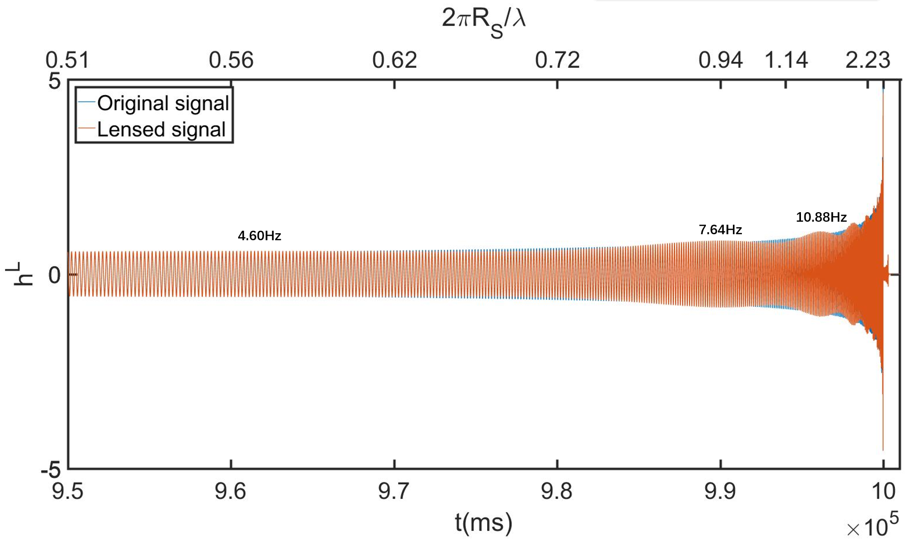
Figure 1 shows the “beat” pattern for the 3-3 $M_{\odot}$ and 30-30 $M_{\odot}$ binary black holes. The point lens masses are 1000 $M_{\odot}$ and 2000 $M_{\odot}$ , and $y$ are settled as 2 and 3, respectively. On the upper $x$ -axis of these figures, we show $2\pi R_{s}/\lambda$ of the signal, which is the criterion of wave region and optical region, and the red lines delineate the boundaries for with condition (10) is satisfied. From these results we can see that the patterns show up when the wavelength is comparable with the Schwarzschild radius of lens, and the positions of peaks before the red line is indicated by equation (12).

To get the coefficients $\alpha$ of equation (12) by fitting apprach, we change the mass of lens from 100 $M_{\odot}$ to 2000 $M_{\odot}$ , and $y$ from 0.8 to 5.0. As an example, we fix $y$ as 5.0, and plot the $f_{peak}-n/M_{L}$ map discussed in section III.1 in Figure 2. We define $\gamma$ as $t_{coal}-t=\gamma\frac{11}{16}t_{d}$ , and it is obvious that the larger the $\gamma$ , the better the linear relationship discussed in equation (12) is. And this figure also indicates that the proportional coefficients in high frequency region $\alpha$ are also valid in low frequency region, as discussed in section II.1 and III.1, which is $\alpha\approx 1.12$ by fitting.

We also test this formula with different sources and different $y$ , e.g., $30-30M_{\odot}$ binary black holes, the lens mass also varies from $100M_{\odot}$ to $2000M_{\odot}$ , and $y$ varies from 1.0 to 5.0. We also fit $\alpha$ by plotting $k-n/\Delta t_{d}$ , and we find that $\alpha$ is also approximate to 1.12. The results are showed in Figure 3.

V. SUMMARY AND OUTLOOK

In this paper, we propose a new method to measure the mass, position and the absolute magnification of gravitational lens for the strong lensed systerm with GW alone. We focus on the “ betat” patterns of lensed GW, and we find the relationship between the frequency of the peaks $f_{p}$ of the envelope , the amplitude ratio of adjacent valleys and peaks $r$ , and the mass $M_{L}$ , position $y$ of gravitational lens: equations (8), (12) , and (14), where equation (8) and (14) is valid for optical region, and equation (12) is valid for both wave and optical region as long as condition (10) is satisfied. Thus by measuring the corresponding frequencies of more than two adjacent peaks, we can obtain $\Delta t_{d}$ from equation (12) or (8). Since the unlensed waveform with the normalized amplitude removed can be easily measured, i.e., $b(t)e^{i(\Phi(t)+\phi_{0})}$ in waveform (13), we can obtain the position of lens $y$ using equation (14), then we can obtain the mass of lens $M_{L}$ , the absolute magnification $\mu$ , and therefore the distance of GW source $D_{L}$ .

The point mass lens model and the BH-BH signals are used to demonstrate our methord. This systerm could be detectered in future ground based detectors.

Refer to caption — (a) 3-3 $M_{\odot}$ binary black hole, $y=2.0$ ,, and $M_{L}=1000M_{\odot}$ .

References

LIGO/Virgo collaborations (2016) B. P. Abbott et al., Phys. Rev. Lett., 116, 061102 (2016), (2016), arXiv:1602.03837 [gr-qc]; Phys. Rev. Lett., 116, 241103 (2016), arXiv:1606.04855 [gr-qc]; Phys. Rev. Lett., 118, 221101 (2017), arXiv:1706.01812 [gr-qc]; Phys. Rev. Lett. 119, 141101 (2017), arXiv:1709.09660 [gr-qc]; Phys. Rev. Lett. 119, 161101 (2017), arXiv:1710.05832 [gr-qc]; Astrophys. J. 851, L35 (2017), arXiv:1711.05578 [astro-ph.HE]; B. P. Abbott et al. (LIGO Scientic, Virgo), Phys. Rev. X 9, 031040 (2019), arXiv:1811.12907 [astro-ph.HE].
P. Schneider, J. Ehlers, and E. E. Falco (1992) P. Schneider, J. Ehlers, and E. E. Falco, Gravitational Lenses (Springer, Berlin, Heidelberg, 1992) p. 560.
Ackermann et al. (2014) Ackermann, M., Albert, A., Atwood, W. B., et al. 2014, ApJ, 793, 64
Nakamura (1998) Nakamura T. T., ”Gravitational Lensing of Gravitational Waves from Inspiraling Binaries by a Point Mass Lens”, Phys. Rev. Lett., 80, 1138 (1998)
Takahashi & Nakamura (2003) Takahashi R., Nakamura T., 2003, ApJ, 595, 1039
Takahashi (2016) Takahashi R., ”Arrival Time Differences between Gravitational Waves and Electromagnetic Signals due to Gravitational Lensing” ApJ, 385, 103 (2017)
Piórkowska, Biesiada & Zhu (2013) Piórkowska A., Biesiada M. & Zhu Z-H. ”Strong gravitational lensing of gravitational waves in Einstein Telescope” JCAP10(2013)022
Biesiada et al. (2014) Biesiada M., Ding X., Piórkowska A. & Zhu Z-H. ”Strong gravitational lensing of gravitational waves from double compact binaries - perspective for the Einstein Telescope” JCAP10(2014)080
Ding, Biesiada & Zhu (2015) Ding X., Biesiada M. & Zhu Z-H., ”Strongly lensed gravitational waves from intrinsically faint double compact binaries - prediction for the Einstein Telescpe” JCAP12(2015)006
Li et al. (2018) Li S-S., Mao S., Zhao Y., Lu Y., ”Gravitational lensing of gravitational waves: A statistical perspective” MNRAS 476, 2220-2229 (2018)
Ng et al. (2018) Ken K. Y. Ng, Kaze W. K. Wong, Tjonnie G. F. Li, & Tom Broadhurst ”Precise LIGO Lensing Rate Predictions for Binary Black Holes” Phys. Rev. D 97, 023012 (2018)
Cao et al. (2014) Zhoujian Cao., Li-Fang Li. & Yan Wang ”Gravitational lensing effects on parameter estimation in gravitational wave detection with advanced detectors” Phys. Rev. D 90, 062003 (2014)
Dai et al. (2017) Liang Dai., Tejaswi Venumadhav. & Kris Sigurdson ”Effect of lensing magnification on the apparent distribution of black hole mergers” Phys. Rev. D 95, 044011 (2017)
Liao et al. (2017) Liao K., Fan X-L., Ding X., Biesiada M. & Zhu Z-H., ”Precision cosmology from future lensed gravitational wave and electromagnetic signals” Nature Comm. 8:1148 (2017)
Hou et al. (2019a) Hou S., Fan X-L., & Zhu Z-H., S. Hou, X.-L. Fan, K. Liao, and Z.-H. Zhu, arXiv:1911.02798 [gr-qc].
Fan et al. (2017) Fan X-L., Liao K., Biesiada M., Piórkowska-Kurpas A., Zhu Z-H., ”Speed of gravitational waves from strongly lensed gravitational waves and electromagnetic signals” , Phys. Rev. Lett. 118, 091102 (2017)
Hou et al. (2019b) S. Hou, X.-L. Fan, and Z.-H. Zhu, Phys. Rev. D 100, 064028 (2019), arXiv:1907.07486 [gr-qc].
Baker & Trodden (2017) Baker, T. & Trodden, M., ”Multi-Messenger Time Delays from Lensed Gravitational Waves” Phys. Rev. D 95, 063512 (2017)
Collett & Bacon (2017) Thomas E. Collett & David Bacon., ”Testing the Speed of Gravitational Waves over Cosmological Distances with Strong Gravitational Lensing” , Phys. Rev. Lett. 118, 091101 (2017)
K. Liao, M. Biesiada, and X.-L. Fan (2019) K. Liao, M. Biesiada, and X.-L. Fan, Astrophys. J. 875, 139 (2019), arXiv:1903.06612 [gr-qc].
Yang et al. (2019) Lilan Yang, Xuheng Ding, Marek Biesiada, Kai Liao, and Zong-Hong Zhu, Astrophys. J. 874, 139 (2019)
Li et al. (2019) Yufeng Li, Xilong Fan, and Lijun Gou, Astrophys. J. 837, 37 (2019)
Li et al. (2018) Kai Liao, Xuheng Ding, Marek Biesiada, Xi-Long Fan, and Zong-Hong Zhu, Astrophys. J. 867, 69 (2018)