Low rank tensor completion with sparse regularization in a transformed domain
Abstract
Tensor completion is a challenging problem with various applications. Many related models based on the low-rank prior of the tensor have been proposed. However, the low-rank prior may not be enough to recover the original tensor from the observed incomplete tensor. In this paper, we prose a tensor completion method by exploiting both the low-rank and sparse prior of tensor. Specifically, the tensor completion task can be formulated as a low-rank minimization problem with a sparse regularizer. The low-rank property is depicted by the tensor truncated nuclear norm based on tensor singular value decomposition (T-SVD) which is a better approximation of tensor tubal rank than tensor nuclear norm. While the sparse regularizer is imposed by a -norm in a discrete cosine transformation (DCT) domain, which can better employ the local sparse property of completed data. To solve the optimization problem, we employ an alternating direction method of multipliers (ADMM) in which we only need to solve several subproblems which have closed-form solutions. Substantial experiments on real world images and videos show that the proposed method has better performances than the existing state-of-the-art methods.
Keywords:
Low rank completion , Truncated nuclear norm , Tensor singular value decomposition , Discrete cosine transformation , Alternating direction method of multipliers (ADMM)1 Introduction
Estimating missing data from very limited information of observed data has attracted considerable interest recently. This problem arises from various kinds of applications in signal processing and machine learning [3, 23, 12, 8], such as image recovery, video denosing, recommender systems, and data mining. However, estimating the missing values without any prior information about the data is usually an ill-posed problem. There are many commonly adopted assumptions which can be divided into local and global information to alleviate the problem. To utilize the local information, the statistical or structural information [4] of the observed data are used to build up the relation between the missing data and the known data, but it is obviously that the approach only focuses on local relations. It is necessary to consider the global structural information of the observed data.
In many real applications, the signals lie in a low dimensional space, for example, the natural images data have a low-rank structure [7, 10, 22]. As a result, the matrix completion problem can be modeled as a low-rank minimization problem
| (1) | ||||
where , rank() denotes the rank of the matrix and is the set of locations corresponding to the observed data. However, the rank function of matrix is a nonconvex and discontinuous function [7], so the resulting (1) is a NP-hard problem. Theoretical studies show that the nuclear norm, i.e., the sum of singular values of a matrix, is the convex surrogate of the rank function [17]. Furthermore, there are some efficient methods to solve the nuclear norm minimization problem [2]. Unfortunately, these nuclear norm methods may lead to suboptimal results, since all the singular values are treated differently when added together and minimized simultaneously while in the rank minimization process all the singular values have the same [7]. Therefore, the matrix truncated nuclear norm (MTNN) [7, 9] was proposed by minimizing the sum of the minimum singular values because the rank of a matrix only depends on the first nonzero singular values. In this way, a more accurate approximation of rank function is obtained, at the same time the empirical research showed that the MTNN approach has much better approximation performances than other methods based matrix nuclear norm [5].
Although these low-rank prior based approaches have obtained good results, additional information could be considered for a more accurate reconstruction. Another thing need to be noted is that the low-rank component always indicates that the real data in practice also have intrinsically sparse property [20, 18]. One possible way is to exploit the sparse information of the complete matrix in a certain domain, such as transform domains where many signals have inherent sparse structures [20]. To describe the sparse property in a certain domain, Dong [5] proposed a general way by applying the transform operation to matrices as an implicit function.
However, dealing with color images and videos by matrix does not exploit the structural information among channels. It is natural to consider extending the matrix completion to tensor completion [14] for such a task. Since there is no perfect definitions for tensor rank and tensor nuclear norm, several types of tensor nuclear norm were proposed. Liu [13] initially proposed the sum of matricized nuclear norm (SMNN) of a tensor, which is defined as
| (2) | ||||
where denotes the matrix of the tensor unfolded along the th mode, e.g., the mode- matricization of , is a parameter which satisfies , and is the original incomplete tensor. Kilmer [11] proposed a novel tensor decomposition method, called the tensor singular value decomposition (T-SVD). Then Zhang [21] proposed a new tubal nuclear norm based on T-SVD, which is defined as the sum of nuclear norms of all frontal slices in the Fourier domain and proofed that it was a convex relaxation to the tensor tubal rank. As a result their optimization model can be written as
| (3) | ||||
where will be introduced in the next section.
The same as which has mentioned in matrix completion, the tensor nuclear norm also minimizes all the singular value at the same level which is unfair to the larger singular values, because the larger singular values always contain much more important information. Then tensor truncated nuclear norm was proposed. Han [6] proposed a tensor truncated nuclear nuclear norm T-TNNS based on MTNN. Xue [19] proposed a tensor truncated nuclear norm T-TNN based on T-SVD, which will be given in next section.
To obtain a more accurate completion performance, we consider the sparse property of the tensor in a transform domain. Here we select the multi-dimensional discrete consine transform (DCT) [24], since signals has a intrinsic sparse property in this transform domain [18]. Further we introduce a -norm regularization term into the objective function to impose local sparsity and to preserve the piecewise smooth property of the reconstructed tensor. Then we solve the objective function by alternating between two steps. The first step is achieved by performing T-SVD to the observed tensor. The second step solves the cost function by the alternating direction method of multipliers (ADMM) [1], which is widely used for solving constrained optimization problems because its guarantee of convergence in polynomial time.
2 Notations and Preliminaries
In this paper, we denote tensors by boldface Euler script letters, e.g., . Matrices are denoted by boldface capital letters, e.g., . Vectors are denoted by boldface lowercase letters, e.g., , and scalars are denoted by lowercase letters, e.g., . We denote as the identity matrix. The field of real numbers and complex numbers are denoted as and , respectively. For a 3D tensor , we denote its -th elements as or and use Matlab commands , and to respectively denote the -th horizontal, lateral and frontal slice. More often, the frontal slice is denoted as . The tube is denoted as . The inner product of and in is defined as , where denotes the transpose of and denotes the matrix trace. The trace of is defined as . The inner product of and in is defined as .
Some norms of tensor and matrix are used. We denote the -norm as and the Frobenius norm as . The matrix nuclear norm is , e.g., the sum of all singular values of matrix .
For tensor , by using the Matlab command fft, we denote as the result of discrete Fourier transform (DFT) [2] of along the third mode, i.e., fft. In the same fashion, we can compute from by ifft using the inverse FFT. In particular we denote as a block diagonal matrix with each diagonal block as the frontal slice of , i.e.,
| (4) |
This bdiag can be seen as an operator which maps the tensor to the block diagonal matrix .
The block circulant matrix corresponding to a tensor is defined as
| (5) |
For tensor , we define
| (6) |
where the operator maps to a matrix of size and is its inverse operator.
Definition 1
Tensor product [21] Let and . Then the tensor-product is defined to be a tensor of size , e.g.,
| (7) |
where denotes the matrix product.
The tensor product can be understood from two perspectives. First, in the original region, it is analogous to the matrix product except that the circular convolution replaces the product operation between the elements. The tensor product reduces to the standard matrix product when . Second, in Fourier domain, it is equivalent to the matrix multiplication, e.g., [15] .
Definition 2
Transpose [21] The transpose of a tensor is the tensor obtained by transposing each of the frontal slice and then reversing the order of transposed frontal slices 2 through , e.g.,
| (8) | ||||
Definition 3
Identity tensor [21] The identity tensor is the tensor whose first frontal slice is the identity matrix, and whose other frontal slices are all zeros.
Definition 4
Orthogonal tensor [21] A tensor is orthogonal if it satisfies
| (9) |
Definition 5
F-diagonal tensor [21] A tensor is called f-diagonal if each of its frontal slices is a diagonal matrix.
Theorem 1

Definition 6
Tensor tubal rank and tensor nuclear norm [19] Let the T-SVD of tensor be . The tensor tubal rank of is defined as the maximum rank among all frontal slices of the f-diagonal , i.e., maxi rank. The tensor nuclear norm is defined as the sum of the singular values in all frontal slices of , i.e.,
| (11) |
According to the definition of FFT function, we carry out fft along the third mode, then we can get a symmetric property between the trace of tensor product and the trace of and [19], i.e.,
| (12) |
The formulation (13) suggests that we can compute the tensor nuclear norm by one matrix SVD in the Fourier domain rather than the complicated T-SVD in the original domain.
Definition 7
where is the inverse fft of , and is a constant, and is the rank of .
Theorem 2
[5] Let be a given matrix and be any non-negative integer with . For any matrices , satisfying , , we have
| (15) |
where denotes the identity matrix of size .
3 Proposed method
In the formulation of our proposed method, the low-rank assumption and the sparse prior are both considered in order to better utilize the structure information of the tensor. Since the truncated nuclear norm can provide a better approximation to rank function in matrix [5], Xue et al. [19] extended this property directly to tensor by defining a new tensor truncated nuclear norm (T-TNN). We employ this T-TNN to model the low-rank prior information in this paper. For the sparse prior, we proposed a new term to describe it. For the reasons mentioned in the introduction section, we assume the original tensor is sparse in the DCT transform domain. Hence the proposed method is named after sparse regularization in a transformed domain, e.g., SRTD. Let denote the forward n-dimensianal DCT, and the transformed tensor is assumed to be sparse.
3.1 Problem formulation
For a tensor , the tensor completion problem can be formulated as the following constrained optimization problem
| (16) | ||||
where and is the original incomplete tensor with observed values on the support . The tensor truncated nuclear norm can be expressed as follows
| (17) | ||||
where is the truncated singular value.
Since formulation (17) is nonconvex, it is difficult to solve it directly. We use Theorem 2 to transform (17) into a convex problem. Combining with (12), (13) and Theorem 2, (17) can be reformulated as
| (18) | ||||
So the formulation (16) becomes
| (19) | ||||
To solve the optimization problem (19), an iterative method alternating between two steps is adopted. In the first step, we compute the T-SVD of a fixed tensor, i.e., , and then and can be derived from and , i.e.,
| (20) |
In the second step, by assuming that and are fixed, we compute from a simplified formulation
| (21) | ||||
ADMM is used to solve (21), and the details will be presented in the next subsection. The overall solution framework for solving (19) is summarized in Algorithm 1.
3.2 Problem reformulation and ADMM
We introduce an auxiliary tensor and reformulate the optimization problem (21) as
| (22) | ||||
Due to the introduction of variable , (22) can be addressed by ADMM. The augmented Lagrangian function of (22) becomes
| (23) | ||||
where and are Lagrange multiplier tensors of the same size with , and is a penalty parameter. Based on the basic framework of ADMM, the optimization problem (23) can be solved by alternatively updating one variable with the others fixed. Specifically, in the th iteration, the variables are updated via the following scheme
| (24) |
where is a predetermined constant to increase the penalty, and is a given upper bound for the penalty.
3.2.1 Update
| (25) | ||||
Here cannot be separated from the other variables since the existence of the transform operator in the last term. However, the Parseval’s theorem [16] indicates that if the transformation is an unitary under Frobenius norm, the energy of the signal is unchanged. According to the Parseval’s theorem and the unitary invariant property of DCT, the last term can be rewritten as
| (26) |
where denotes the corresponding inverse transform of .
Hence, we have
| (27) | ||||
The above problem has a closed-form solution, given by
| (28) |
where is the SVT operator defined in definition 7.
3.2.2 Update
| (29) | ||||
The above problem has a closed-form solution, given by
| (30) |
where is the element-wise soft thresholding operator [2], defined by
| (31) |
3.2.3 Update
| (32) | ||||
Therefore, by setting the derivative of (32) to zero, we obtain a closed-form solution as follows:
| (33) | ||||
In addition, the observed data should keep constant in each iteration, i.e.,
| (34) |
3.2.4 Update
| (35) |
3.2.5 Update
| (36) |
3.2.6 Update
| (37) |
The whole procedure to solve the problem (22) is summarized in Algorithm 2.
4 Experiments
In this section, several experiments are conducted to demonstrate the efficiency of proposed SRTD method. The compared methods are:
It is necessary to explain the difference between proposed SRTD method and compared methods: MTNN considers transforming the tensor data to matrix data during experiments, which doesn’t employ the correlation between channels; T-TNN employs tensor truncated nuclear norm defined by T-SVD, which only considers the low rank information of recovered data; T-TNNS considers the tensor truncated nuclear norm which is defined by the sum of matricized nuclear norm and sparse regularization, but it may can’t utilize the channels information as well as the proposed SRTD.
All the experiments are performed in Matlab R2016a on Windows 10, with an Intel Core i5 CPU @2.50GHz and 8 GB Memory.
The Peak Signal-to-Noise ration (PSNR) is used to describe and evaluate the performance of the recovered images and videos, which is defined as follows
| (38) |
| (39) |
where is the total number of data in a tensor, i.e. for tensors considered in Definition 1, and we assume that the maximum pixel value in is 255. It is obviously that the higher the PSNR, the better the recovery performance.
4.1 Parameter setting
To make sure the comparison is fair, we choose the best parameter for each algorithm. For MTNN, the parameters are set as , , , and , which have been discussed in [5]. For T-TNN, to better illustrate its performance, the random sampling rata (SR) at 50% is tested. For T-TNNS, the parameter is set as 0.19 to obtain it’s best performance, and the other parameters are set as the same with [6]. For the proposed SRTD, there is another parameter need to be discussed. We test for
at SR = 50%. And the PSNR of image 3 and image 7 in Table 1 are shown in Figure 2.
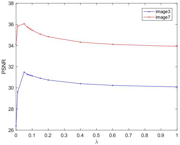
From Figure 2, we can see that when , the optimization function of SRTD is reduced to the objection function of T-TNN. We can directly see that the PSNR of SRTD method is better than T-TNN method when range into (0,1). The PSNR reaches its peak when is around 0.05, so we set in our tests. We do not know the real rank of the incomplete tensor and there is no prior information for us to determine the number of truncated singular values, so following a common practice we manually test the rank range into (1,20) to find the best value in each case.
4.2 Image recovery with random mask
A color image can be seen as a 3D tensor usually with a low-rank structure, we first consider ten color images with size of . The test sampling rates (SRs) are set as 30%, 40% and 50%. We show the completion result in the Table 1. To verify the efficiency of proposed SRTD method, we further randomly select ten color images from Berkeley Segmentation database11 1 http://www.eecs.berkeley.edu/Research/Projects/CS/vision/bsds/ with size . We test the same SRs at 30%, 40% and 50%, and show the completed results in the Table 2.
| No. | Images | SR | PSNR | |||
| MTNN | T-TNN | T-TNNS | SRTD | |||
| 1 | ![[Uncaptioned image]](1911.08082v1/new1.jpg) |
30% | 26.48 | 26.35 | 27.49 | |
| 40% | 26.86 | 27.96 | 28.82 | |||
| 50% | 27.12 | 29.56 | 30.09 | |||
| 2 | ![[Uncaptioned image]](1911.08082v1/new2.jpg) |
30% | 30.89 | 29.22 | 31.28 | |
| 40% | 31.68 | 30.80 | 32.75 | |||
| 50% | 32.19 | 32.32 | 34.11 | |||
| 3 | ![[Uncaptioned image]](1911.08082v1/new3.jpg) |
30% | 26.31 | 23.32 | 26.95 | |
| 40% | 27.21 | 25.58 | 28.82 | |||
| 50% | 28.06 | 27.62 | 30.43 | |||
| 4 | ![[Uncaptioned image]](1911.08082v1/new4.jpg) |
30% | 30.27 | 30.74 | 31.10 | |
| 40% | 31.20 | 33.02 | 33.18 | |||
| 50% | 32.01 | 35.11 | 35.05 | |||
| 5 | ![[Uncaptioned image]](1911.08082v1/new5.jpg) |
30% | 29.98 | 27.77 | 30.30 | |
| 40% | 30.67 | 29.50 | 31.70 | |||
| 50% | 31.22 | 31.34 | 33.07 | |||
| 6 | ![[Uncaptioned image]](1911.08082v1/new6.jpg) |
30% | 24.02 | 23.28 | 24.88 | |
| 40% | 24.35 | 24.60 | 26.04 | |||
| 50% | 24.63 | 25.95 | 27.25 | |||
| 7 | ![[Uncaptioned image]](1911.08082v1/new7.jpg) |
30% | 30.64 | 30.75 | 31.56 | |
| 40% | 31.23 | 32.68 | 32.91 | |||
| 50% | 31.79 | 34.42 | 34.37 | |||
| 8 | ![[Uncaptioned image]](1911.08082v1/new8.jpg) |
30% | 28.05 | 26.39 | 28.18 | |
| 40% | 28.59 | 28.11 | 29.53 | |||
| 50% | 29.07 | 29.83 | 30.85 | |||
| 9 | ![[Uncaptioned image]](1911.08082v1/new9.jpg) |
30% | 25.15 | 25.21 | 26.45 | |
| 40% | 25.46 | 26.90 | 27.91 | |||
| 50% | 25.85 | 28.81 | 29.56 | |||
| 10 | ![[Uncaptioned image]](1911.08082v1/new10.jpg) |
30% | 27.43 | 27.97 | 29.41 | |
| 40% | 28.11 | 30.04 | 31.34 | |||
| 50% | 28.74 | 32.29 | 33.33 | |||
| No. | Images | SR | PSNR | |||
| MTNN | T-TNN | T-TNNS | SRTD | |||
| 1 | ![[Uncaptioned image]](1911.08082v1/pic1.jpg) |
30% | 24.35 | 24.00 | 26.75 | |
| 40% | 25.40 | 26.64 | 29.16 | |||
| 50% | 26.38 | 29.38 | 31.50 | |||
| 2 | ![[Uncaptioned image]](1911.08082v1/pic2.jpg) |
30% | 26.43 | 28.68 | 28.24 | |
| 40% | 26.98 | 30.87 | 30.37 | |||
| 50% | 27.53 | 33.48 | 32.80 | |||
| 3 | ![[Uncaptioned image]](1911.08082v1/pic3.jpg) |
30% | 24.05 | 25.62 | 26.37 | |
| 40% | 24.82 | 28.50 | 28.97 | |||
| 50% | 25.56 | 30.89 | 31.47 | |||
| 4 | ![[Uncaptioned image]](1911.08082v1/pic4.jpg) |
30% | 25.60 | 26.67 | 29.33 | |
| 40% | 26.95 | 26.36 | 31.41 | |||
| 50% | 27.82 | 32.54 | 33.87 | |||
| 5 | ![[Uncaptioned image]](1911.08082v1/pic5.jpg) |
30% | 27.07 | 25.97 | 28.53 | |
| 40% | 27.97 | 28.37 | 30.58 | |||
| 50% | 28.77 | 30.62 | 32.35 | |||
| 6 | ![[Uncaptioned image]](1911.08082v1/pic6.jpg) |
30% | 20.11 | 23.01 | 22.58 | |
| 40% | 20.85 | 25.51 | 24.99 | |||
| 50% | 21.46 | 28.53 | 27.82 | |||
| 7 | ![[Uncaptioned image]](1911.08082v1/pic7.jpg) |
30% | 23.47 | 24.46 | 26.54 | |
| 40% | 24.45 | 27.07 | 28.82 | |||
| 50% | 25.33 | 29.76 | 31.05 | |||
| 8 | ![[Uncaptioned image]](1911.08082v1/pic8.jpg) |
30% | 20.56 | 21.56 | 22.30 | |
| 40% | 21.01 | 23.51 | 24.10 | |||
| 50% | 21.44 | 25.63 | 26.21 | |||
| 9 | ![[Uncaptioned image]](1911.08082v1/pic9.jpg) |
30% | 30.65 | 29.53 | 32.88 | |
| 40% | 31.45 | 31.89 | 34.93 | |||
| 50% | 32.31 | 34.54 | 36.94 | |||
| 10 | ![[Uncaptioned image]](1911.08082v1/pic10.jpg) |
30% | 29.88 | 29.92 | 32.32 | |
| 40% | 30.78 | 32.59 | 34.49 | |||
| 50% | 31.66 | 35.36 | 36.69 | |||
We can easily see the proposed SRTD performances better than compared methods from Table 1 and Table 2. Moreover, in most cases the PSNR of T-TNN, T-TNNS are better than MTNN, which shows that it is better to use tensors rather than matrices to deal with color images.
Figure 3 shows the six test color images recovered by MTNN, T-TNN, T-TNNS and SRTD respectively at SR . To better show the details of the images, we magnify a significant region for each completed images. Both from the visual quality and the value of PSNR, we can see that the proposed SRTD has a better performance.


We further choose image 3 and image 4 from Table 1, and we set the SR range from 10% to 90%. The result is shown in Figure 4, we can directly see from the PSNR value that the performance of SRTD is always better than that of MTNN, T-TNN and T-TNNS, even when the SR becomes very low. However, with the SR decreasing, the performance of T-TNNS decays quickly.


4.3 Image recovery with text mask
In this part, we consider images which are corrupted by a text mask. It is a difficult task to remove the text, since the text is not randomly distributed in the image and it may cover some very important texture information. The text removal experiments results are shown in Figure 5 and Figure 6.


It can be seen from the recovered images that the proposed algorithm can recover the missing pixels by the text mask noise very well. Moreover, we can see that the PSNR of the proposed SRTD is higher than that of MTNN, T-TNN and T-TNNS. Specifically, for the first image, the PSNR are 27.45, 27.81, 29.63 and 30.03 respectively for MTNN, T-TNN, and T-TNNS. For the second image, the PSNR are 22.23, 23.42, 23.68 and 24.21 respectively for MTNN, T-TNN, and T-TNNS. From both the PSNR values and visual effect, it can be demonstrated that the proposed method has a better performance.
4.4 Video recovery with random mask
Here we choose a gray basketball video which can been seen as a 3D tensor from YouTube.com with size . The first two modes of the video correspond to the spatial variety, and the last mode corresponds to time changes. We set the SRs at 35 and 25 respectively. We compare the recovered PSNR value of proposed SRTD with T-TNN and T-TNNS, and show the contrast results of the 20th frame in Figure 7 and Figure 8. Again, we observe that the performance of proposed SRTD is better than T-TNN and T-TNNS in PSNR values and visual effect.


5 Conclusion
In this paper, we proposed a tensor completion approach SRTD based on the low-rank and sparse prior. In detail, we used the tensor truncated nuclear norm based on T-SVD rather than the tensor nuclear norm used in most of the existing methods, which can be regarded as a direct extension of matrix truncated nuclear norm. -norm is used to describe the sparse prior of the tensor in a DCT domain, which is a general way to model the sparse property of tensors. A constrained optimization problem is formulated and then solved by ADMM iteration scheme. Experimental results showed that the proposed SRTD method performs better than MTNN, T-TNN and T-TNNS.
reference
References
- [1] S. Boyd, N. Parikh, E. Chu, B. Peleato, and J. Eckstein, Distributed optimization and statistical learning via the alternating direction method of multipliers. Found Trends Mach Learn. 3(1)(2011) 1-122.
- [2] J-F. Cai, E. J Candès, and Z. Shen, A singular value thresholding algorithm for matrix completion, SIAM J. Optimiz. 20(4)(2010) 1956-1982.
- [3] A. Cichocki, D. Mandic, L. De. Lathauwer, G. Zhou, Q. Zhao, C. Caiafa, and H. A. Phan, Tensor decompositions for signal processing applications: from two-way to multiway component analysis, IEEE Signal Process. Mag. 32(2)(2015) 145-163.
- [4] D. Coupier, A. Desolneux, and B. Ycart, Image denosing by statistical area thresholding, Math Imaging Vis. 22(2-3)(2015) 183-197.
- [5] J. Dong, Z. Xue, J. Guan, Z-F. Han, and W. Wang, Low rank matrix completion using truncated nuclear norm and sparse regularizer, Signal Processing: Image Commu. 68(2018) 76-87.
- [6] Z-F. Han, C-S. Leung, L-T. Hung, and H-C. So, Sparse and truncated Nuclear Norm Based Tensor Completion, Neural Process.Lett. 45(2017) 729-743.
- [7] Y. Hu, D. Zhang, J. Ye, X. Li and X. He, Fast and accurate matrix completion via truncated nuclear norm regularization, IEEE Trans Pattern Anal. Mach. 35(9)(2013) 2117-2130.
- [8] T.-Y. Ji, T.-Z. Huang, X.-L. Zhao, T.-H. Ma, G Liu, Tensor completion using total variation and low-rank matrix factorization, Information Sciences 326(2016) 243-257.
- [9] T.-Y. Ji, T.-Z. Huang, X.-L. Zhao, T.-H. Ma, L.-J. Deng, A non-convex tensor rank approximation for tensor completion, Applied Mathematical Modelling 48(2017) 410-422.
- [10] T.-X. Jiang, T.-Z. Huang, X.-L. Zhao, T.-Y. Ji, L.-J. Deng, Matrix factorization for low-rank tensor completion using framelet prior, Information Sciences 436(2018) 403-417.
- [11] M. E. Kilmer, K. Braman, N. Hao, and R. C. Hoover, Third-order tensors as operators on matrices: a theoretical and computational framework with applications in imaging, SIAM J. Matrix Anal. Appl. 34(1)(2013) 148-172.
- [12] W. Li, L. Zhao, D. Xu, and D. Lu, Efficient image completion method based on alternating direction theory, IEEE International Conference on Image Processing. 73(2019) 12-21.
- [13] J. Liu, P. Musialski, P. Wonka, and J. Ye, Tensor completion for estimating missing values in visual data, IEEE Trans.Patt.Anal. 35(1)(2013) 208-220.
- [14] Z. Long, Y. Liu, L. Chen, and C. Zhu, Low rank tensor completion for multiway visual data. Signal Processing. 155(2019) 301-316.
- [15] C. Lu, J. Feng, Y. Chen, W. Liu, Z. Lin, and S. Yan, Tensor robust principal component analysis with a new tensor nuclear norm. IEEE Trans. Patt.Anal. (2019).
- [16] N. Merhav, and R. Kresch, Approximate convolution using DCT coefficients multipliers, IEEE Trans. Circuits Syst. video Technol. 8(4)(1998) 378-385.
- [17] B. Recht, M. Fazel, and P. A. Parrilo, Guaranteed minimum-rank solutions of linear matrix equations via nuclear norm minimization, SIAM Rev. 52(3)(2010) 471-501.
- [18] J. Wright, Y. Ma, J. Mairal, G. Sapiro, T. S. Hung, and S. Yan, Sparse representation for computer vision and pattern recognition. Proc. IEEE. 98(6)(2010) 1031-1044.
- [19] S. Xue, W. Qiu, F. Liu, and X. Jin, Low-rank tensor completion by truncated nuclear norm regularization, 24th International Conference on Pattern Recognition IEEE. (2018) 1-6.
- [20] J. Yang, J. Wright, T. S. Huang, and L. Yu, Image super-resolution via sparse representation, IEEE Trans.Image Process. 19(11)(2010) 2861-2873.
- [21] Z. Zhang, G. Ely, S. Aeron, N. Hao and M. Kilmer, Novel methods for multilinear data completion and de-nosing based on tensor-SVD. IEEE conf. Computer Vision and Pattern Recognition. (2014) 3842-3849.
- [22] Y.-B. Zheng, T.-Z. Huang,T.-Y. Ji, X.-L. Zhao, T.-X. Jiang, and T.-H. Ma, Low-rank tensor completion via smooth matrix factorization, Applied Mathematical Modelling 70(2019) 677-695.
- [23] M. Zhou, Y. Liu, Z. Long, L. Chen, and C. Zhu, Tensor rank learning in CP decomposition via convolutional neural network, Signal Process: Image Commun. 326(2015).
- [24] Z. Zhu, S-K. A. Yeung, and B. Zeng, In search of "Better-than-DCT" unitary Transforms for encoding of residual signals, IEEE Signal Process Lett. 17(11)(2010) 961-964.