Delay-Aware Wireless Network Coding in Adversarial Traffic
Abstract
We analyze a wireless line network employing wireless network coding. The two end nodes exchange their packets through relays. While a packet at a relay might not find its coding pair upon arrival, a transmission cost can be reduced by waiting for coding with a packet from the other side. To strike a balance between the reduced transmission cost and the cost incurred by the delay, a scheduling algorithm determining either to transmit an uncoded packet or to wait for coding is needed. Because of highly uncertain traffic injections, scheduling with no assumption of the traffic is critical. This paper proposes a randomized online scheduling algorithm for a relay in arbitrary traffic, which can be non-stationary or adversarial. The expected total cost (including a transmission cost and a delay cost) incurred by the proposed algorithm is at most times the minimum achievable total cost. In particular, the proposed algorithm is universal in the sense that the ratio is independent of the traffic. With the universality, the proposed algorithm can be implemented at each relay distributedly (in a multi-relay network) with the same ratio. Moreover, the proposed algorithm turns out to generalize the classic ski-rental online algorithm.
I Introduction

There has been a dramatic proliferation of research on wireless network coding. The wireless network coding can substantially reduce the number of transmissions by exploiting the broadcast nature of wireless medium, resulting in power saving. Illustrated in Fig. 1-(a), two end nodes and exchange their respective packets and belonging to the Galois field through a relay. The conventional communication technique (without network coding) requires four transmissions (two for each packet). Leveraging the wireless network coding, only three transmissions are required; precisely, nodes and send packets and to the relay, and the relay broadcasts the scalar-linear combination (by bitwise XOR over ) to both end nodes. Each end node (for ) can recover its desired packet by subtracting (over ) packet it already has from packet it receives. In general, the wireless network coding can save up to 50% of transmissions as long as the number of relays in a line network in Fig. 1-(b) (as also called the reverse carpooling [2]) is large.
To benefit from the wireless network coding, a relay has to create sufficient coded packets; however, a coded packet at the relay can be created only when packets from both sides are available. Precisely, a relay in Fig. 1-(b) maintains two queues and storing packets from both sides, respectively. If both queues are non-empty, then the relay can construct coded packets by combining packets from both queues. However, what should the relay do if only one queue is non-empty? Should the relay wait for coding in the future or just transmit uncoded packets from the non-empty queue? To fully realize the advantage of the wireless network coding would incur packet delays, whereas always transmitting uncoded packets to minimize the delays causes a larger number of transmissions. Therefore, a scheduling algorithm for determining when to code is crucial.
The scheduling problem for a single-relay network as in Fig. 1-(a) under stationary stochastic traffic has been investigated leveraging stochastic control techniques, like Lyapunov theory (e.g., [3]) or Markov decision processes (e.g., [4]). All the prior solutions fail to generalize to non-stationary or adversarial (worst-case) traffic. In particular, they cannot be implemented at each relay distributedly in a multi-relay network with provable performance guarantees. However, non-stationary or adversarial traffic has gained increasing importance in recent years. On one hand, external traffic injections at nodes or can arbitrarily be generated by their sources, following no particular probabilistic assumption. On the other hand, the relay cannot expect the scheduling algorithms employed by nodes and to follow a stationary probabilistic distribution. In particular, [5] claimed that the adversarial traffic is a better traffic model. Because of those practical issues, the research on the adversarial traffic has attracted much attention in recent years (e.g., [6]). Although network coding design for adversarial channels has been an active area (e.g., [7]), little attention was given to the adversarial traffic in network-coding-enabled networks. To fill the gap, this paper aims to develop a universal scheduling algorithm for arbitrary traffic with a provable performance guarantee.
Moreover, note that the ski-rental problem [8] is a classic problem in an adversarial setting, where for each day a skier decides either to buy a ski or to continue renting a ski without knowing the skier’s last vacation, e.g., the day when the snow melts. The ski-rental setting has been exploited in several works (e.g., [9]) for managing delays under some uncertainties. This paper shows that the proposed scheduling algorithm can solve generalized ski-rental scenarios.
I-A Contributions
Our main contribution lies in designing and analyzing scheduling for delay-aware wireless network coding in the adversarial traffic. The objective is to minimize a total cost, including a transmission cost and a delay cost, for each relay. To reach the goal, we show that our problem can be cast into a linear program. Leveraging primal-dual techniques [10] for the linear program, we propose a randomized online scheduling algorithm for each relay in a multi-relay network. In particular, the proposed algorithm can guarantee that the worst-case ratio between the expected total cost incurred by the proposed online algorithm and that incurred by an optimal offline algorithm is (asymptotically) . In addition to the theoretical worst-case analysis, the average-case analysis is conducted via computer simulations. Moreover, it turns out that the proposed algorithm can generalize the classic ski-rental algorithm to several scenarios.
I-B Related works
Scheduling design for network-coding-enabled networks has been extensively explored from various perspectives. Most scheduling works with network coding aimed to maximize throughput (i.e., stability regions), e.g., [11, 12, 13, 14, 15, 16, 17, 18, 19, 20]. While [11, 12, 13, 14] considered static network environments and solved deterministic optimization problems, [15, 16, 17, 18, 19, 20] considered dynamic network environments and solved dynamic optimal control problems. Moreover, several scheduling works with network coding investigated delays, e.g., [21, 22, 23]. In addition to the throughput or delays, some prior works analyzed other utilities or constraints when network coding is enabled, e.g., [24] maximized a video reception quality and [25] considered a Quality-of-Service (QoS) constraint.
The most relevant works on the trade-off between delays and power consumption (with wireless network coding) in relay networks are [3, 4]. While [3] proposed a scheduling algorithm using Lyapunov techniques, [4] showed the optimality of a threshold-type scheduling algorithm using Markov decision processes. All those prior solutions were based on stochastic models with some stationary assumptions but cannot apply to non-stationary settings, especially in multi-relay networks. In contrast, we explore the trade-off in non-stationary settings.
II System overview
II-A Network model
Consider a wireless line network in Fig. 1-(b). The two end nodes and send and packets (in ), respectively, to each other through shared relay nodes. Divide time into slots and index them by . Suppose that a perfect schedule of wireless links is given, so that during each slot each node can transmit some packets under a transmission constraint without any interference. The interference-free link schedule can be achieved by existing medium access control (MAC) protocols, e.g., scheduled TDMA used in [4], CSMA proposed by [26], or coded ALOHA proposed by [27]. In fact, our design can work with any MAC protocol (see Remark 14 later).
Consider a relay in Fig. 1-(b). The relay constructs queues for storing those packets that arrive at the relay but cannot be transmitted immediately upon arrival. As shown in Fig. 1-(b), the relay maintains two queues and for packets generated by nodes and , respectively. At the beginning of each slot , there are new packets arriving at queue and new packets arriving at queue . By we define an arrival pattern for the relay. The arrival pattern depends on the number of packets transmitted in the previous slot by its neighboring nodes. The arrival pattern is arbitrary, which can be non-stationary or even adversarial.
Let and be the number of packets at queues and , respectively, immediately after the packet arrivals in slot . If and , then the relay idles in slot . If and , then the relay transmits some coded packets (under the transmission constraint) by combining (over ) packets from both queues. Transmitting the coded packets can save the number of transmissions22 2 To save the number of transmissions, both neighboring nodes of the relay must be able to decode the coded packets transmitted by the relay. To that end, we leverage the reverse carpooling technique [2]. Each node (including both end nodes and all relay nodes) keeps packets it transmitted previously for a while, so that when it receives a coded packet, it can decoded the coded packet. See Footnote 3 later for the amount of time to keep a packet it previously transmitted. Moreover, each relay employs the decode-and-forward mechanism, where it decodes before re-encoding and transmitting packets. without incurring any delay. After transmitting the coded packets, if only one queue is non-empty and the relay can transmit more packets in that slot, then the relay has two options for those packets at the non-empty queue: to transmit some uncoded packets from the non-empty queue or to idle with the hope of receiving packets at the empty queue in the next slot (for coding). While always to transmit uncoded packets minimizes the delays, always to idle minimizes the number of transmissions by coding. To strike a balance between the delays and the number of transmissions, the best decision is unclear when exactly one of the queues is non-empty.
To investigate the best decision for each slot, we let be the relay’s decision on the number of packets (including both uncoded and coded packets) transmitted in slot . We assume that the broadcast channel from the relay to its neighboring nodes is noiseless. This simple model facilitates to explore the delays for coding in the arbitrary arrival pattern. In fact, our design can extend to adversarial ON-OFF channels (see Remark 24 later). Under the noiseless assumption, the queueing dynamics is
for all and . For example, if , , and , then the relay transmits three coded packets combining three packets from queues and each, and transmits one uncoded packet from queue ; moreover, if , then .
A scheduling algorithm for the relay specifies decision for each slot . A scheduling algorithm is called an offline scheduling algorithm if arrival pattern is given as a prior. In contrast, a scheduling algorithm is called an online scheduling algorithm if arrival pattern (along with the numbers and of packets) is unavailable; instead, it knows the present arrivals and only, for each slot .
II-B Problem formulation
To capture the trade-off between the delays and the number of transmissions, we define a holding cost and a transmission cost as follows. Suppose that holding a packet at the end of a slot incurs a cost of one unit. Moreover, suppose that each packet transmission takes a constant cost of units33 3 The transmission cost is the weight (i.e., importance) between the transmission power of a packet and the delay of a packet for one slot, depending on applications. If the transmission power is critical, then cost is larger; on the contrary, cost is smaller. Moreover, we are going to minimize the total transmission cost plus the total holding cost as in Eq. (1). In this context, the value of is the maximum number of slots for that a packet can delay. If a packet delays for more than slots, then it incurs more holding cost than the saving of transmission cost by coding. Thus, for a delay-sensitive application, we can set the value of to be its deadline constraint., where we assume that transmitting a coded packet incurs the same transmission cost as transmitting an uncoded packet. See Remark 6 for non-consistent costs for transmitting coded and uncoded packets. Moreover, we consider the case when the value of is greater than one44 4 Following Footnote 3, scheduling for the case when is trivial: if only one queue is non-empty, then the relay always transmits uncoded packets but never waits for coding, because holding a packet for a slot incurs more cost than the saving of transmission cost by coding. Thus, this paper focuses on the case when , where packets can delay for some slots. .
Given arrival pattern , we define a total cost under scheduling algorithm by
| (1) |
where the first term reflects the cost of transmitting packets in slot and the other terms reflects the cost of delaying all remaining packets for one slot. Since we consider the finite numbers and , the minimum achievable total cost is finite.
We aim to develop an online scheduling algorithm such that the total cost is minimized for all possible arrival patterns . However, without knowing arrival pattern (along with the total numbers and of packets) in advance, an online scheduling algorithm is unlikely to achieve the minimum total cost (obtained by an optimal offline scheduling algorithm). We characterize our online scheduling algorithm in terms of the competitiveness against an optimal offline scheduling algorithm, defined as follows.
Definition 1.
For arrival pattern , let be the minimum total cost for all possible (offline) scheduling algorithms . Then, an online scheduling algorithm is called -competitive if
for all possible arrival patterns , where is called the competitive ratio of the online scheduling algorithm .
Remark 2.
A -competitive online scheduling algorithm guarantees that the resulting total cost is at most times the minimum total cost, regardless of arrival patterns . Thus, while a -competitive online scheduling algorithm can be implemented at each relay in the multi-relay network in a distributed way, it guarantees the competitive ratio for each relay.
We aim to design and analyze an online scheduling algorithm for minimizing the competitive ratio.
III One-sided adversarial traffic
We start with a fixed number of packets waiting for coding; in particular, this section focuses on the following setting:
- 1.
Queue has all (with ) packets initially, i.e., and for all .
- 2.
Queue is injected by arbitrary traffic with a total of packets.
- 3.
The relay can transmit any number of packets in each slot.
The setting is referred to as the one-sided adversarial traffic. With the first and second assumptions, we can focus on a fixed number of packets at queue waiting for coding, while capturing the key feature of the adversarial arrival pattern at queue . In fact, the first assumption is practical as well for bursty traffic at queue . Section IV will also generalize to two-sided adversarial traffic. Note that, under the first assumption, the relay never delays the packets at queue for minimizing the total cost. The third assumption is made for delivering a clear insight into our innovation. Lemma 15 will analyze the maximum number of transmissions required by the proposed online scheduling algorithm; moreover, Section IV-E will extend to a transmission constraint.
III-A Overview of our methodology
This section provides an overview of our methodology (leveraging primal-dual techniques [10] for linear programs):
- 1.
We propose linear program (4) for optimally solving our scheduling problem in the offline fashion (with arrival pattern as a prior).
- 2.
- 3.
We analyze the objective value (of linear program (4)) computed by Alg. 1 through a solution (produced also by Alg. 1) to the dual of the linear program. We show that the objective value computed by Alg. 1 is no more than times that dual objective value. Then, the duality theory yields that the objective value computed by Alg. 1 is no more than times the minimum objective value (of linear program (4)).
- 4.
- 5.
Section III-B formulates the linear program (as a primal program) and its dual program. While Section III-C proposes Alg. 1 for solving the primal program and the dual program in the online fashion, Section III-D analyzes the solution produced by Alg. 1. Leveraging the solution produced by Alg. 1, Section III-E proposes Alg. 2 for solving our scheduling problem and analyzes its expected total cost.
III-B Primal-dual formulation
Given arrival pattern , this section casts the offline scheduling problem (under the one-sided adversarial traffic) into a linear program. To that end, we introduce some variables:
- •
: the number of packets at queue transmitted without coding.
- •
: the number of packets at queue at the end slot of .
If the relay decides to transmit uncoded packets at queue , then it must55 5 If one of those uncoded packets is transmitted in slot , then the total cost in Eq. (2) increases by (for holding the packet for slots). For minimizing the total cost, the uncoded packets are optimally transmitted in slot 1. transmit the uncoded packets in slot . Thus, the total cost in Eq. (1) under the one-sided adversarial traffic can be expressed by
| (2) |
where the first term is the cost of transmitting all packets at queue , the second term is the cost of transmitting the uncoded packets at queue in slot 1 (i.e., transmitting coded packets at queue is free), and the last term is the cost incurred by holding the packets at queue .
By removing the constant from Eq. (2), we have the following scheduling problem.
Problem 3.
Under the one-sided adversarial traffic, develop a scheduling algorithm for the packets at queue such that the cost is minimized.
Remark 4.
This remark shows that the classic ski-rental problem [8] is a special case of our Problem 3. In the ski-rental problem, a skier arrives at a resort on day 1 with no ski. For each day, the skier decides either to buy a ski or to rent a ski. If the skier buys a ski in a day, then the skier does not have to rent a ski after that day. While renting a ski for a day takes one dollar, buying a ski takes dollars. The skier will stay at the resort for days until the last vacation day. The goal is to minimize the buying cost plus the total renting cost. Given the instance of the ski-rental problem, we construct an instance of our Problem 3. We construct one packet for each queue, i.e., . We construct a packet staying at queue in slot 1 (corresponding to the skier). We construct a packet arriving at queue in slot (corresponding to the last vacation day). Next, we link a skier’s decision with a relay’s decision. While the skier rents a ski on day if and only if the relay idles in slot , the skier buys a ski on day if and only if the relay transmits the packet at queue without coding in slot . While the skier does not have to make decisions after day , the relay also does not have to make decisions after slot (because the relay can transmit a coded packet in slot if the packet at still stays at that queue in slot ). With the link between the ski-rental problem and our Problem 3, variable in Problem 3 can indicate if the skier buys a ski, and variable in Problem 3 can indicate if the skier rents a ski on day . Suppose that holding the packet at queue for a slot takes one dollar, and that transmitting an uncoded packet from queue takes dollars. Then, the value of in Problem 3 can represent the buying cost plus the total renting cost. Thus, the ski-rental problem equivalently becomes our Problem 3. In other words, the ski-rental problem is a special case () of our Problem 3.
Remark 5.
Following Remark 4, this remark shows that our Problem 3 is a generalization of the ski-rental problem. We can think of each packet at queue as a skier and think of a slot when a packet arrives at queue as the day when a skier has to leave. Moreover, buying a ski takes dollars while renting a ski for a day takes one dollar. With the transformation, Problem 3 considers a group of skiers (i.e., the packets at queue ) with potentially different last vacation days (i.e., the arriving slots at queue ). Those skiers cooperatively make a buying or renting decision on each day for minimizing the total buying cost plus the total renting cost.
Remark 6.
If transmitting a coded packet incurs a cost of units and transmitting an uncoded packet incurs a different cost of units with , then the total cost in Eq. (1) becomes
where the term is the extra cost for transmitting the coded packets. Then, we can replace cost in Problem 3 with . Note that . If were higher than , then transmitting a coded packet by combining two packets would not save any cost from transmitting two uncoded packets. The rest of the paper focuses on the constant cost without loss of generality.
Next, we propose the following integer program for optimally solving Problem 3 in the offline fashion:
Integer program:
| (3a) | |||||
| s.t. | (3b) | ||||
| (3c) | |||||
where is the total number of packets arriving at queue until slot . The constraint in Eq. (3b) is because for each slot the number of packets at queue is at least , where packets at queue are transmitted without coding in slot and at most packets at queue are transmitted with coding by slot .
Next, by relaxing the integrality constraint in Eq. (3c) to real numbers, we obtain the following linear program.
Linear program (primal program):
| (4a) | |||||
| s.t. | (4b) | ||||
| (4c) | |||||
After the relaxation, a feasible fractional solution for in linear program (4) can no longer represent a decision for the number of packets at queue transmitted without coding (but an integral solution for in linear program (4) can). In fact, the next lemma shows that the relaxation has no integrality gap.
Proof.
From Lemma 7, Problem 3 can be optimally solved in polynomial time if arrival pattern is given in advance: Solve for variable in linear program (4); then, transmit uncoded packets in slot 1. After transmitting the uncoded packets in slot , all other packets at queue always wait for packets at queue for coding.
Next, while Section III-B proposes an online algorithm for sub-optimally solving for variable without knowing arrival pattern in advance, Section III-D analyzes the objective value in Eq. (4a) computed by the proposed online algorithm by its dual program. Thus, we refer to linear program (4) as a primal program and express its dual program as follows.
Dual program:
| (5a) | |||||
| s.t. | (5b) | ||||
| (5c) | |||||
III-C Primal-dual algorithm
This section proposes a primal-dual algorithm in Alg. 1 for obtaining a solution to primal program (4) and dual program (5). The primal-dual algorithm does not have arrival pattern as a prior; instead, it can obtain the present arrivals and only, for each slot .
Alg. 1 initializes all variables (in Lines 1 and 1) at the beginning of slot 1. Obtaining the present arrivals and at the beginning of each new slot , Alg. 1 updates all variables for slot . For updating the value of , Alg. 1 introduces a set of auxiliary variables (initialized in Line 1). The intuition66 6 The intuition here is just our idea of solving for variable in the online fashion, but is not scheduling decisions for packets. Section III-E will cast a value of variable to a randomized decision. behind updating variable and in Lines 1, 1, and 1 is following: We can imagine the value of to be a probability of transmitting the -th (counted from the head of queue ) packet at queue without coding. Precisely, for each slot , Line 1 increases the value of for those packets potentially staying at queue :
- •
A total of packets arrive at queue by slot , yielding at most coded packets until . As such, Line 1 considers , for until , because only the -th packet until the -th packet might wait at queue in slot , but other packets have been transmitted with coding by slot .
- •
The constant used in Line 1 is specified as the function of transmission cost in Line 1 for satisfying the dual constraint in Eq. (5b). Then, Line 1 sets the value of to be that of , counting all packets at queue .
Moreover, Alg. 1 introduces another set of auxiliary variables for all , and updates the value of to be that of (in Line 1) in slot for satisfying the constraint in Eq. (4b). Again, the value of is set to be that of in Line 1, counting all packets at queue . In addition, the value of is updated to be one in Line 1 for maximizing the dual objective value in Eq. (5a) subject to the constraints in Eq. (5c).
We want to emphasize that the solution produced by Alg. 1 can be non-integral. The solution is just a feasible solution to primal program (4) but can no longer represent the number of packets at queue transmitted without coding. However, by exploiting the solution produced by Alg. 1, Section III-E will propose a randomized online scheduling algorithm for solving Problem 3. The underlying idea is that the intermediate fractional solution for in primal program (4) produced by Alg. 1 in each slot can be transformed to a probability of transmitting an uncoded packet in that slot.
III-D Analysis of Alg. 1
This section analyzes the proposed Alg. 1. Since the values of all variables can be updated by Alg. 1 in each slot, the following proofs use , , , , , , , , to represent the corresponding values at the beginning (before update) of slot ; use , , , , , , , , to represent the corresponding values at the end (after update) of slot . Note that , , , , , , , , is the solution produced by Alg. 1. In fact, Alg. 1 will not update any variable after slot (see Remark 10 later), where we recall that the value of is the transmission cost.
The next lemma establishes the primal feasibility of Alg. 1.
Proof.
See Appendix B. ∎
The next lemma establishes the dual feasibility of Alg. 1. For proving the lemma, we define the increment (under Alg. 1) of the value of in slot by . From [10], we can obtain that for all ; moreover, if , then for . That is, forms a geometric sequence, with the initial value of and the ratio of .
Proof.
First, the dual constraint in Eq. (5c) holds obviously according to Lines 1 and 1. Second, we will show that the value of in Eq. (5b) computed by Alg. 1 is less than or equal to . Note that Line 1 updates the value of to be one if the condition in Line 1 holds. Thus, it suffices to show that the condition in Line 1 fails at the end of slot , i.e., the value of is zero for all .
If in slot , then we can obtain
where (a) is because the sequence is the geometric sequence with the initial value of and the ratio of . Thus, the value of for all is zero since the condition in Line 1 fails. ∎
Remark 10.
Theorem 11.
Proof.
Let be the increment (under Alg. 1) of the primal objective value in Eq. (4a) in slot and let be that of the dual objective value in Eq. (5a) in slot . Appendix C establishes that
for all . Let and be the primal and dual objective values, respectively, computed by Alg. 1. Then, and ; therefore, the result follows since
where the last inequality is due to the weak duality [10]. ∎
III-E Randomized online scheduling algorithm
Leveraging Alg. 1, this section proposes a randomized online scheduling algorithm in Alg. 2. For each slot , Alg. 2 transmits coded packets (in Line 2) by combing packets left at queue and the new arriving packets at queue . Then, to decide whether to transmit uncoded packets for each slot, Lines 2 - 2 and 2 update the values of and in the same way as Alg. 1 does. In addition, Alg. 2 uses another variable (in Line 2) to record the value of at the beginning (before update in Line 2) of each slot. Let be the value of at the end of slot .
At the beginning of slot , Line 2 chooses a random number from a continuous uniform distribution between 0 and 1. According to Lines 2 - 2, if there exists a such that , then the relay transmits an uncoded packet in slot . Note that, if there are multiple ’s such that , then the relay transmits multiple uncoded packets in slot , until the present value of is greater than or equal to (as in Line 2).
Let () be the increment of the value of in slot . The idea behind Alg. 2 is that, with the random choice of , the expected number of uncoded packets transmitted in slot is exactly .
Theorem 12.
Proof.
We show that the expected cost of transmitting uncoded packets by Alg. 2 is , which is the value of the first term in Eq. (4a) computed by Alg. 1. Moreover, we show that the expected number of packets left at queue at the end of slot under Alg. 2 is less than or equal to , which is the value of the second term in Eq. (4a) computed by Alg. 1. Thus, the expected cost incurred by Alg. 2 is less than or equal to the primal objective value in Eq. (4a) computed by Alg. 1. Then, the result immediately follows from Theorem 11. See Appendix D for details. ∎
Remark 13.
Recall that a competitive ratio is the worst-case ratio for all possible cases (i.e., arrival patterns ) and recall that the ski-rental problem is a case of our Problem 3 (from Remark 4). Thus, the minimum achievable competitive ratio for our problem is no higher than that for the ski-rental problem. Because the minimum achievable competitive ratio for the ski-rental problem is [8] and Alg. 2 can also achieve that competitive ratio, we can conclude that Alg. 2 achieves the minimum achievable competitive for Problem 3.
Remark 14.
The next lemma investigates the maximum number of uncoded packets per slot required by Alg. 2.
Lemma 15.
Alg. 2 transmits at most three uncoded packets in each slot.
Proof.
Since is the geometric sequence with the initial value of and the ratio of for all , we have
Moreover, because of , , and (from the assumption for the one-sided traffic), we have . Thus, at most three ’s such that , i.e., Alg. 2 transmits at most three uncoded packets in each slot. ∎
To analyze the computational complexity of Alg. 2, we note that there are at most iterations in Lines 2 - 2. Moreover, there are at most iterations in Lines 2 - 2 (by Lemma 15). Since (from the assumption for the one-sided traffic), the computational complexity of Alg. 2 is . As the value of grows, the computational complexity increases but the competitive ratio in Theorem 12 decreases.
IV Two-sided adversarial traffic
This section relaxes the first assumption in the one-sided adversarial traffic by allowing arbitrary traffic at both queues and . We start with the scenario where only packets at a queue can wait for coding; in particular, this section starts with the following setting:
- 1.
The packets at queue can wait for coding but those at queue are transmitted immediately upon arrival.
- 2.
The relay can transmit any number of packets in each slot.
This setting is referred to as the two-sided adversarial traffic. This model can make us focus on decisions for a queue while capturing the key feature of the two-sided adversarial traffic. In fact, the first assumption is practical as well when the traffic generated by node is urgent and even cannot delay for more than one slot (e.g., urgent events in intelligent transportation systems or ultra-reliable low-latency communications (URLLC) [28] in 5G). Later, Section IV-D will relax the first assumption by extending to the general case when packets at both queues can wait for coding. Moreover, Section IV-E will relax the second assumption by imposing a transmission constraint.
We introduce some variables similar to Section III:
- •
: indicate if the -th packet at queue is transmitted without coding upon arrival, where if the packet is transmitted without coding; otherwise;
- •
: the number of packets at queue at the end of slot .
We have the following problem similar to Problem 3.
Problem 16.
Under the two-sided adversarial traffic, develop a scheduling algorithm for the packets at queue such that the cost is minimized.
Remark 17.
Section IV-A discusses ideas underlying another primal-dual formulation that will be proposed by Section IV-B for solving Problem 16. With the new primal-dual formulation, Section IV-C proposes a primal-dual algorithm for solving Problem 16 in the online fashion.
IV-A Ideas underlying the primal-dual formulation
The next example shows that an immediate extension from linear program (4) along with Alg. 1 cannot solve Problem 16 with the competitive ratio in Theorem 11.
Example 18.
Suppose that two packets arrive at queue in slots 1 and 3, respectively, and no packet arrives at queue . Assume transmission cost . In this case, the optimal solution to Problem 16 is and , i.e., both packets at queue are optimally transmitted without coding upon arrival. In particular, the optimal solution satisfies the following linear program (similar to linear program (4)).
Linear program (primal program):
| (6a) | |||||
| s.t. | (6b) | ||||
| (6d) | |||||
The associated dual program can be expressed as
Dual program:
| (7a) | |||||
| s.t. | (7c) | ||||
Applying the idea behind Alg. 1, we would update and update until the dual constraint in Eq. (7c) becomes tight. Given , the constant is . In slot 1, update to be and update to bo one. In slot 2, update to be and update to be one. Because the dual constraint in Eq. (7c) becomes tight in slot 2, we cannot update any variable since slot 3; in particular, we cannot update when the second packet arrives at queue . Thus, the second packet waits forever, yielding an infinite holding cost.
To tackle the issue in the above example, the next example proposes another primal-dual formulation.
Example 19.
Note that an optimal solution for and in linear program (6) also satisfies the following linear program, where we use and to indicate if the first packet and second packet, respectively, stay at queue at the end of slot .
Linear program (primal program):
| (8a) | |||||
| s.t. | (8b) | ||||
| (8d) | |||||
While expressing variable in Eq. (6a) by in Eq. (8a), we substitute the original constraints in Eqs. (6b) and (6d) by the constraints in Eqs. (8b) and (8d). The associated dual program can be expressed as
Dual program:
| (9a) | |||||
| s.t. | (9b) | ||||
| (9d) | |||||
Follow the idea behind Alg. 1 as discussed in Example 18. In slot 1, update to be and update to be one. In slot 2, update to be one and update to be one. In slot 3, update to be and update to be one. In slot 4, update to be one and update to be one. The updating process can achieve the competitive ratio in Theorem 11.
The above example implies that the idea of Alg. 1 can solve Problem 16 with the same competitive ratio, if we can formulate a linear program with constraints for each individual packet (like Eqs. (8b) and (8d)) instead of those for all arriving packets (like Eqs. (6b) and (6d)). In this context, we introduce additional variables: let indicate if the -th packet stays at queue at the end slot , where if it does and otherwise. For each slot , the value of is either zero or one, where implies that the -th packet at queue is transmitted with coding by slot and implies that the packet is either transmitted without coding by slot or stays at queue at the end of slot . By the next example, we emphasize that the constraints should be carefully considered.
Example 20.
Suppose that two packets arrive at queue in slots 1 and 2, respectively, and one packet arrives at queue in slot 3. Assume transmission cost . In this case, the optimal solution to Problem 16 is and . Next, given the optimal decision for the packet at queue (i.e., optimally transmitted with coding), we consider constraints for each packet at queue as follows:
- •
Slot : A packet arrives at queue in slot . Thus, we can obtain .
- •
Slot : The other packet arrives at queue in slot . Thus, we can obtain and .
- •
Slot : A packet arrives at queue . Since we are given that the packet at queue optimally codes with a packet at queue , two options are following: (1) , , i.e., the first packet at queue is transmitted with coding, and the second packet either is transmitted without coding or waits in slot ; (2) , .
- •
Slot : No packet arrives at both queues. Thus, if and , then and ; otherwise, and .
We calculate the minimum value of subject to the two possible constraints, i.e., forming two different linear programs:
- •
Consider the constraints of for , and for : The optimal solution is and , while the minimum objective value is .
- •
Consider the constraints of for , and : The optimal solution is and , while the minimum objective value is .
Thus, only the second set of constraints is correct. The idea underlying the correct set of constraints is that the first packet waits for a longer time (for coding) than the second packet does.
Let be the set of indices such that the value of in slot is specified to be greater than or equal to one. Let . Our goal is to identify a correct set of constraints such that the solution to minimize the cost (in Problem 16) subject to the set is an optimal solution to Problem 16. Example 20 suggests that, when a packet arrives at queue in slot , a correct set of constraints in slot can be obtained by removing the most recent packet in set of the previous slot. The argument will be confirmed in the next section.
IV-B Primal-dual formulation
With the idea developed in Example 20, we propose an algorithm in Alg. 3 for identifying a correct set of constraints. Line 3 initiates set in slot to be set of the previous slot. When a packet arrives at queue in slot , Line 3 adds the corresponding index to set . Line 3 introduces a variable to indicate the available packets at queue for coding; precisely, Line 3 sets the value of variable to be the present arrivals at queue . Since Line 3, if (i.e., there is a packet at queue ) and (i.e., there is a packet at queue ), then Line 3 removes index (i.e., the most recent packet in set as in Line 3) from set and Line 3 removes one packet from queue .
We formulate a linear program subject to the set produced by Alg. 3 as follows.
Linear program (primal program):
| (10a) | ||||
| s.t. | (10b) | |||
Proof.
We prove by induction. See Appendix E for details. ∎
The dual program of primal program (10) is following.
Dual program:
| (11a) | |||||
| s.t. | (11c) | ||||
IV-C Primal-dual algorithm
Note that Alg. 3 can learn a correct set of constraints for each slot in the online fashion. Leveraging the online feature, we develop a primal-dual algorithm in Alg. 4 for solving Problem 16 in the online fashion. For each slot , Alg. 4 updates those ’s in the set in Lines 4 - 4. The updating process is similar to that in Alg. 1.
Using the same arguments as those in the proofs of Lemmas 8 and 9, the next lemma establishes the feasibility of the solution produced by Alg. 4.
Similar to Theorem 11, the next theorem shows that Alg. 4 can achieve the same competitive ratio as Alg. 1 does.
Theorem 23.
Proof.
See Appendix F. ∎
Then, similar to Alg. 2, we can transform the solution produced by Alg. 4 to a randomized online scheduling algorithm for managing the delay-award coding decision at queue . In particular, the scheduling algorithm can also achieve the same expected competitive ratio as that in Theorem 12, approaching when cost is large enough.
IV-D Scheduling both queues
This section extends Alg. 4 to the case when both queues and can wait for each other. In this context, we propose a waiting-coding queueing system consisting of a waiting queue and a coding queue at the relay. While queue stores those packets that can wait for coding, queue stores those packets that can find coding pairs at the waiting queue immediately upon arrival.
Precisely, let and be the number of packets at queue and queue , respectively, at the end of slot . If the packets at queue belong to queue , then the (i.e., the number of packets arriving at the original queue ) new arriving packets enter queue at the beginning of slot , and
- 1.
if , then the new arriving packets enter queue at the beginning of slot ;
- 2.
if , then only out of the new arriving packets enter queue at the beginning of slot , but the remaining packets enter queue at the beginning of slot .
In contrast, if the packets at queue belong to queue , then the waiting-coding queueing system operates in the opposite way. In other words, while packets entering queue are transmitted (with coding) immediately upon arrival, packets entering queue need scheduling decisions. With the transformation, the waiting-coding queueing system becomes the previously discussed model where only packets at queue can wait for coding. Thus, the randomized online scheduling algorithm associated with Alg. 4 can apply to the waiting-coding queueing system with the expected competitive ratio in Theorem 12. Furthermore, Section V will demonstrate the superiority of the proposed scheduling algorithm and the proposed waiting-coding queueing system via computer simulations.
IV-E A transmission constraint
Recall that Alg. 4 might transmit more than one packet in a slot (but less than three uncoded packets, as shown in Lemma 15). This Section considers a transmit constraint: the relay can transmit at most one packet in each slot. According to Section IV-D, we can focus on scheduling packets at queue while all packets at queue are transmitted immediately upon arrival.
Under the transmission constraint, if more than one packet arrive at a queue, then those additional packets (except for one of them) cannot be processed in the arriving slot for any scheduling algorithm. Thus, without loss of generality, we can further assume that at most one packet can arrive at each queue in each slot. If more than one packet arrives at a queue, we can just move them to the following slots, so that at most one packet arrives at that queue. With that assumption, we analyze the number of uncoded packets required by the randomized online scheduling algorithms (like Alg. 2) associated with Alg. 4: following the proof of Lemma 15, the number of uncoded packets transmitted in slot is
where the inequality is because: (1) at most packets (as in the proof of Lemma 9) in set that can be updated by Line 4 of Alg. 4 in slot ; (2) the -th most recent packet in set has been updated by Line 4 of Alg. 4 for at least times since its arrival; (3) the value of is if the -th packet is updated by Line 4 of Alg. 4 for times.
We emphasize that, by the above analysis, the randomized online scheduling algorithm might need two transmissions in a slot, i.e., one potential coded packet plus one potential uncoded packet. To make the randomized online scheduling algorithm perform under the constraint of at most one transmission, we revise Alg. 4 as follows: the updates in Lines 4 - 4 perform only when no packet arrives at queue . That is because, if a packet arrives at queue , the relay has to transmit a coded packet; thus, stop updating those variables for transmitting an uncoded packet. Following the line in [29, Theorem 5], the randomized online scheduling algorithm associated with the revised Alg. 4 can also achieve the same expected competitive ratio of when cost is large enough. Moreover, Section V will validate the revised randomized online scheduling algorithm via computer simulations.
Remark 24.
We remark that the revised randomized online scheduling algorithm can also solve the adversarial ON-OFF channel, also by stopping updating when the channel is OFF.
V Numerical studies
We have analyzed the proposed randomized online scheduling algorithm in the worst-case scenario; in contrast, we investigate the proposed algorithm in the average-case scenario by computer simulations in this section.
First, we simulate a single-relay network (as in Fig. 1-(a)) where packets arrive at queues and according to the i.i.d. Bernoulli distributions with means and , respectively, where and are the Gaussian random variables (for adding some noises to the Bernoulli arrivals) with means and , respectively, and variance . Moreover, the relay can transmit at most one packet for each slot. We compare the proposed scheduling algorithm (i.e., the randomized online scheduling algorithm associated with Alg. 4 along with the waiting-coding queueing system in Section IV-D and the stopping mechanism in Section IV-E) with threshold-type scheduling algorithms, where the relay transmits an uncoded packet in a slot if (in the original queueing system) a queue is empty and the non-empty queue size is over its threshold in that slot. The optimized-threshold scheduling algorithm was proposed in [4] for minimizing the long-run average cost in the stochastic environment. However, deriving an optimal threshold for each queue needs the statistics and , i.e., the optimized-threshold scheduling algorithm is an offline scheduling algorithm. Fig. 2 displays the ratio between the total cost (in 10,000 slots) incurred by the proposed scheduling algorithm and that incurred by the optimized-threshold scheduling algorithm. We can observe that the ratio for the proposed scheduling algorithm is at most 1.35 (in Fig. 2-(a) when and ). That is, the proposed algorithm performs much better than what we analyzed in the worst-case scenario (with the expected competitive ratio of ). In addition, Fig. 2 also displays the ratio between the total cost incurred by the -threshold scheduling algorithm and that incurred by the optimized-threshold scheduling algorithm, where the -threshold is an online scheduling algorithm with the constant threshold and was analyzed in [3]. According to Fig. 2, our algorithm significantly outperforms the -threshold scheduling algorithm. Moreover, We can observe that the ratio (for a fixed and a fixed ) decreases as the variance increases. That is because the ratio in Fig. 2-(a) decreases when the expected arrival rate at queue moves toward 0.5 and the expected arrival rate at queue in Figs. 2-(b) and 2-(c) (i.e., ) moves toward 0.5 (because of the truncation of the Gaussian variable to 0 and 1) when the variance increases.


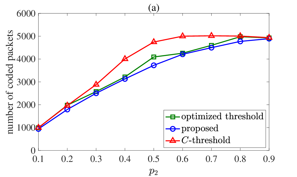
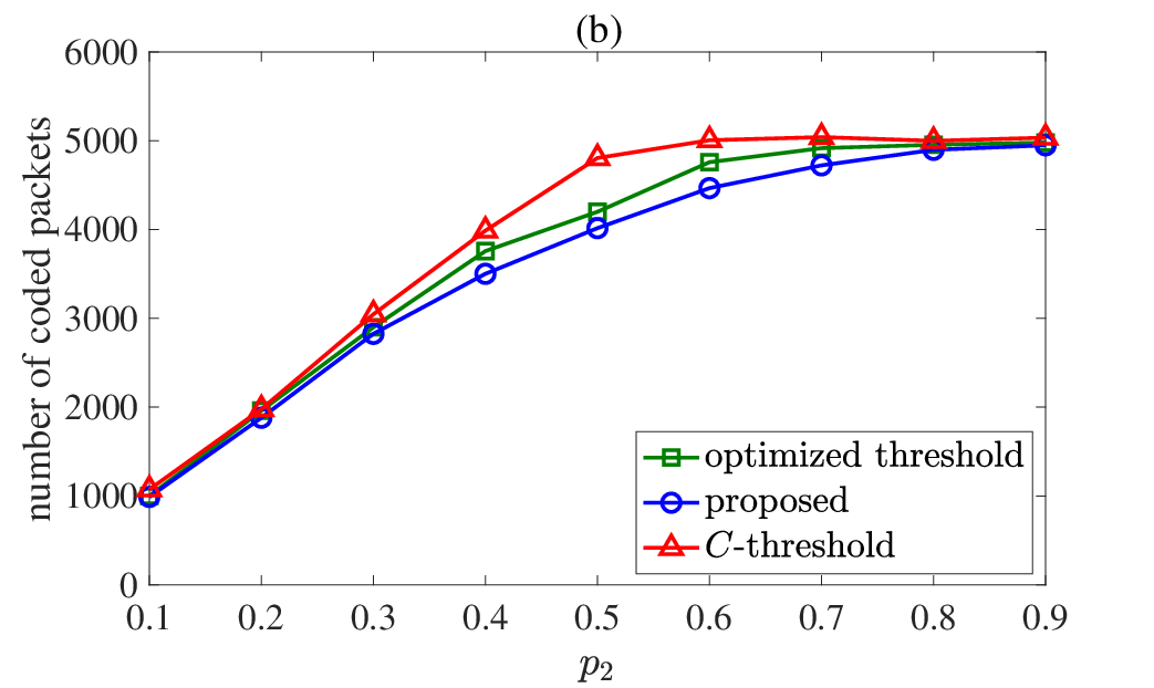
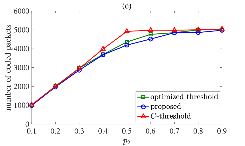
Second, we investigate the coding overheads incurred by the three scheduling algorithms. Fig 3 displays the number of coded packets when (i.e., for the case in Fig. 2-(a)). We can observe that while the proposed scheduling algorithm yields less coded packets than the optimized-threshold scheduling algorithm, the -threshold scheduling algorithm yields more than that. That is, while the proposed scheduling algorithm is a little conservative (in waiting for coding), the -threshold scheduling algorithm waits too long. That is why the proposed scheduling algorithm and the -threshold scheduling algorithm cannot minimize the total cost.
Third, we simulate multi-relay networks where external packets arrive at the two end relays according to the i.i.d. Bernoulli distributions. While each relay can transmit at most one packet for each slot, a received packet from the other relay in a slot cannot be processed until the next slot. Fig. 4-(a) displays the ratio of total costs (with respect to the optimized-threshold scheduling algorithm) when there are two relays and both relays take transmission costs and , respectively. The optimized-threshold scheduling algorithm identifies a threshold for each queue by exhaustive search for minimizing the total cost among all possible thresholds. We want to emphasize that an optimal scheduling for the two-relay network is still unclear. In particular, the optimized-threshold scheduling algorithm might not minimize the long-run average cost in this case, though its great performance has been demonstrated in [4] by computer simulations. We can observe that the ratios for the proposed scheduling algorithm and the -threshold scheduling algorithm in Fig. 2-(a) and Fig. 4-(a) are almost the same. In addition, Fig. 4-(a) also displays the ratio for the sub-optimized-threshold scheduling algorithm, which identifies a threshold for each queue by exhaustive search for minimizing the total cost subject to the condition that all left queues have the same threshold and all right queues do as well. We can observe that the sub-optimized-threshold scheduling algorithm can achieve almost the same total cost as the optimized-threshold scheduling algorithm does. Thus, we compared the proposed scheduling algorithm with the sub-optimized-threshold scheduling algorithm when there are more than two relays and all relays take the same transmission cost . Figs. 4-(b) and Figs. 4-(c) displays the ratio with respect to the sub-optimized-threshold scheduling algorithm. We can observe that the ratio is insensitive to the numbers of relays; in particular, the proposed scheduling algorithm still significantly outperforms the -threshold scheduling algorithm.


VI Concluding remarks
In this paper, we treated a wireless line network employing wireless network coding. The inherent trade-off between packet delays and transmission power consumption under adversarial traffic was studied. In particular, we developed a randomized online scheduling algorithm. The proposed scheduling algorithm not only can theoretically guarantee the expected competitive ratio of for each relay, but also can numerically approach the minimum total cost (including a delay cost and a transmission cost) by computer simulations; moreover, the proposed scheduling algorithm can solve more general ski-rental settings.
While this paper focused on line networks, some discussions on extending to more general networks are following. Consider a relay with multiple line networks traversing, where the two end nodes of each line network exchange their packets. If the relay can transmit one packet in each slot for each line network (as in Section IV-E), then the proposed scheduling algorithm can immediately apply to each line network individually. However, if a relay has a transmission constraint on the total number of transmissions for all line networks, then linear program (10) needs another constraint for specifying that the total number of transmissions cannot be over that transmission constraint. That is an interesting future work. To solve the problem, the prior work [30] (considering a “box constraint”) might be helpful.
Some problems are still open as follows. This paper focused on the worst-case analysis. To theoretically analyze the proposed algorithm in the average-case scenario is interesting and can help understand why it has a great performance in the simulation results. Moreover, we analyzed the competitive ratio of the proposed algorithm in the waiting-coding queueing system; however, the competitive ratio in the original queueing system is still undiscovered. Finally, a MAC protocol is given to this paper. Joint scheduling design of MAC and coding would be a promising future topic.
Appendix A Proof of Lemma 7
Let and be an optimal solution to linear program (4). Note that by Eqs. (4b) and (4c). Let . Suppose that the optimal solution is fractional. We prove by contradiction, according to the following two cases.
- 1.
- 2.
By these contradictions, we conclude that the optimal solution to the linear program is integral.
Appendix B Proof of Lemma 8
Appendix C and in the proof of Theorem 11
We derive and as follows.
- 1.
- 2.
If for , then and since all variables keep unchanged.
The above two cases conclude that
for all .
Appendix D Proof of Theorem 12
First, we compare the expected cost of transmitting uncoded packets by Alg. 2 with the term of the primal objective value in Eq. (4a) computed by Alg. 1. Note that, for a given , there must exist ’s such that , i.e., Alg. 2 transmits uncoded packets in slot ; in addition, according to [29], Alg. 2 transmits one more uncoded packet with probability . Thus, the expected number of uncoded packets transmitted by Alg. 2 in slot is ; moreover, the expected total number of uncoded packets transmitted by Alg. 2 is . We can obtain that the expected cost of transmitting uncoded packets by Alg. 2 is , which is exactly the value of the first term of the primal objective value in Eq. (4a) computed by Alg. 1.
Appendix E Proof of Theorem 21
The proof of the theorem needs the following technical lemma.
Proposition 25.
Given some and such that for all , the optimal objective value of the linear program
| s.t. | ||||
is .
Proof.
We compute the minimum objective value of the linear program via its dual program:
| s.t. | ||||
Since and , we can obtain ; thus, the dual objective value is bounded above by
The equality in the above equation is achievable by setting to be one for all . Therefore, according to the duality theory, we can conclude that the optimal value of the linear program is . ∎
Next, we prove the theorem by induction on and . First, when , linear program (10) obviously can solve Problem 16. Suppose that, when and , linear program (10) can solve Problem 16. Next, we show that linear program (10) can also solve Problem 16 when is , , or . We will focus on the case of , while the other cases just follow the same arguments.
By we denote the arrival pattern obtained by removing a packet arriving at queue in slot and a packet arriving at queue in slot from arrival pattern . By we define the minimum cost in Problem 16 under arrival pattern . Let be the slot when the -th packet arrives at queue . Let indicate a packet arriving at queue in the slot closest to . Then, we can express as
| (13) |
where the first term manages the -th packet arriving at queue (by slot ) and the first packet at queue : if , then the -th packet at queue optimally waits for coding with the first packet at queue ; otherwise, both packets are optimally transmitted immediately (without coding) upon arrival. The second term expresses the minimum cost in Problem 16 when the -th packet at queue and the first packet at queue are both removed from arrival pattern .
By the induction hypothesis, linear program (10) can solve . Particularly, for arrival pattern , we assume that Alg. 3 produces constraints for (for some 77 7 If generated by Alg. 3 is infinity, then we can arbitrarily choose a large number as according to Proposition 25) and . By Proposition 25, we can express in Eq. (13) as
| (14) |
where is the remaining cost incurred by the packets arriving at queue after slot . Similarly, we can express in Eq. (13) by
| (15) |
for , and
| (16) |
By Proposition 25 again, the minimum objective value in linear program (10) under arrival pattern can be expressed by
| (17) |
From Eqs. (13) - (17), it suffices to show that
for all . By removing the common terms from both sides of the above equation, it suffices to show that
| (18) |
for all .

For brevity, for a fixed in Eq. (18), we denote by and for ; denote by for and . See Fig. 5 for illustrating notations and . Let . With the set of notations, Eq. (18) can be simplified as
| (19) |
To verify Eq. (19), note (see Fig. 5 for example) that
| (20) | ||||
| (21) |
Then, Eq. (19) can be confirmed by the following cases.
- 1.
- 2.
Then, we complete the proof.
Appendix F Proof of Theorem 23
References
- [1] Y.-P. Hsu and A. Sprintson, “Opportunistic Network Coding: Competitive Analysis,” Proc. of IEEE NetCod, pp. 191–196, 2012.
- [2] M. Effros, T. Ho, and S. Kim, “A Tiling Approach to Network Code Design for Wireless Networks,” Proc. of IEEE ITW, pp. 62–66, 2006.
- [3] E. C. Ciftcioglu, Y. E. Sagduyu, R. A. Berry, and A. Yener, “Cost-Delay Tradeoffs for Two-Way Relay Networks,” IEEE Trans. Wireless Commun., vol. 10, no. 12, pp. 4100–4109, 2011.
- [4] Y.-P. Hsu, N. Abedini, N. Gautam, A. Sprintson, and S. Shakkottai, “Opportunities for Network Coding: To Wait or Not to Wait,” IEEE/ACM Trans. Netw., vol. 23, no. 6, pp. 1876–1889, 2015.
- [5] A. Borodin, J. Kleinberg, P. Raghavan, M. Sudan, and D. P. Williamson, “Adversarial Queueing Theory,” Proc. of ACM STOC, vol. 96, pp. 376–385, 1996.
- [6] Q. Liang and E. Modiano, “Network Utility Maximization in Adversarial Environments,” Proc. of IEEE INFOCOM, pp. 594–602, 2018.
- [7] A. Ravagnani and F. R. Kschischang, “Adversarial Network Coding,” IEEE Trans. Inf. Theory, vol. 65, no. 1, pp. 198–219, 2018.
- [8] A. R. Karlin, C. Kenyon, and D. Randall, “Dynamic TCP Acknowledgement and Other Stories about ,” Proc. of ACM STOC, pp. 502–509, 2001.
- [9] G. Lee, W. Saad, M. Bennis, A. Mehbodniya, and F. Adachi, “Online Ski Rental for ON/OFF Scheduling of Energy Harvesting Base Stations,” vol. 16, no. 5, pp. 2976–2990, 2017.
- [10] N. Buchbinder and J. S. Naor, The Design of Competitive Online Algorithms via a Primal-Dual Approach. Now Publishers, Inc., 2009, vol. 3, no. 2-3.
- [11] A. ParandehGheibi, A. Ozdaglar, M. Effros, and M. Médard, “Optimal Reverse Carpooling over Wireless Networks-A Distributed Optimization Approach,” Proc. of IEEE CISS, pp. 1–6, 2010.
- [12] D. Traskov, M. Heindlmaier, M. Médard, and R. Koetter, “Scheduling for Network-Coded Multicast,” IEEE/ACM Trans. Netw., vol. 20, no. 5, pp. 1479–1488, 2012.
- [13] T. Wiese, M. Riemensberger, and W. Utschick, “Scheduling for Network-Coded Multicast with Interference,” IEEE Trans. Signal Process., vol. 64, no. 9, pp. 2245–2254, 2016.
- [14] H. Seferoglu and A. Markopoulou, “Network Coding-Aware Queue Management for TCP Flows over Coded Wireless Networks,” IEEE/ACM Trans. Netw., vol. 22, no. 4, pp. 1297–1310, 2014.
- [15] N. Moghadam, H. Li, H. Zeng, and L. Liu, “Lyapunov Scheduling and Optimization in Network Coded Wireless Multicast Network,” IEEE Trans. Veh. Technol., vol. 67, no. 6, pp. 5135–5145, 2018.
- [16] T. Ho and H. Viswanathan, “Dynamic Algorithms for Multicast with Intra-Session Network Coding,” IEEE Trans. Inf. Theory, vol. 55, no. 2, pp. 797–815, 2009.
- [17] A. Eryilmaz, D. S. Lun, and B. T. Swapna, “Control of Multi-Hop Communication Networks for Inter-Session Network Coding,” IEEE Trans. Inf. Theory, vol. 57, no. 2, pp. 1092–1110, 2011.
- [18] W.-C. Kuo and C.-C. Wang, “Robust and Optimal Opportunistic Scheduling for Downlink Two-Flow Network Coding with Varying Channel Quality and Rate Adaptation,” IEEE/ACM Trans. Netw., vol. 25, no. 1, pp. 465–479, 2016.
- [19] C. Fragiadakis, G. S. Paschos, L. Georgiadis, and L. Tassiulas, “Dynamic Wireless Network Coding with Overhearing and Variable Channel Rates,” IEEE J. Sel. Areas Commun., vol. 33, no. 2, pp. 185–198, 2014.
- [20] N. M. Jones, B. Shrader, and E. Modiano, “Distributed CSMA with Pairwise Coding,” Proc. of IEEE INFOCOM, pp. 2094–2102, 2013.
- [21] I.-H. Hou, “Broadcasting Delay-Constrained Traffic over Unreliable Wireless Links with Network Coding,” IEEE/ACM Trans. Netw., vol. 23, no. 3, pp. 728–740, 2014.
- [22] M. Saif, A. Douik, and S. Sorour, “Rate Aware Network Codes for Cloud Radio Access Networks,” IEEE Trans. Mobile Comput., vol. 18, no. 8, pp. 1898–1910, 2018.
- [23] B. T. Swapna, A. Eryilmaz, and N. B. Shroff, “Throughput-Delay Analysis of Random Linear Network Coding for Wireless Broadcasting,” IEEE Trans. Inf. Theory, vol. 59, no. 10, pp. 6328–6341, 2013.
- [24] C. Li, H. Xiong, J. Zou, and D. O. Wu, “Joint Dynamic Rate Control and Transmission Scheduling for Scalable Video Multirate Multicast Over Wireless Networks,” IEEE Trans. Multimedia, vol. 20, no. 2, pp. 361–378, 2017.
- [25] M. S. Al-Abiad, M. J. Hossain, and S. Sorour, “Cross-Layer Cloud Offloading With Quality of Service Guarantees in Fog-RANs,” IEEE Trans. Commun., vol. 67, no. 12, pp. 8435–8449, 2019.
- [26] J. Ni, B. Tan, and R. Srikant, “Q-CSMA: Queue-Length-Based CSMA/CA Algorithms for Achieving Maximum Throughput and Low delay in Wireless Networks,” IEEE/ACM Trans. Netw., vol. 20, no. 3, pp. 825–836, 2011.
- [27] E. Paolini, G. Liva, and M. Chiani, “Coded Slotted ALOHA: A Graph-Based Method for Uncoordinated Multiple Access,” IEEE Trans. Inf. Theory, vol. 61, no. 12, pp. 6815–6832, 2015.
- [28] A. Azari, M. Ozger, and C. Cavdar, “Risk-Aware Resource Allocation for URLLC: Challenges and Strategies with Machine Learning,” IEEE Commun. Mag., vol. 57, no. 3, pp. 42–48, 2019.
- [29] Y.-H. Tseng and Y.-P. Hsu, “Online Energy-Efficient Scheduling for Timely Information Downloads in Mobile Networks,” Proc. of IEEE ISIT, pp. 1022–1026, 2019.
- [30] N. Buchbinder and J. Naor, “Online Primal-Dual Algorithms for Covering and Packing,” Mathematics of Operations Research, vol. 34, no. 2, pp. 270–286, 2009.