Scale Invariance of the Homentropic Inviscid Euler Equations with Application to the Noh ProblemPreprint: LA-UR 19-31605
Abstract
We investigate the inviscid compressible flow (Euler) equations constrained by an ”isentropic” equation of state (EOS), whose functional form in pressure is an arbitrary function of density alone. Under the aforementioned condition, we interrogate using symmetry methods the scale-invariance of the homentropic inviscid Euler equations. We find that under general conditions, we can reduce the inviscid Euler equations into a system of two coupled ordinary differential equations. To exemplify the utility of these results, we formulate two example scale-invariant, self-similar solutions. The first example includes a shock-free expanding bubble scenario, featuring a modified Tait EOS. The second example features the classical Noh problem, coupled to an arbitrary isentropic EOS. In this case, in order to satisfy the conditions set forth in the classical Noh problem, we find that the solution for the flow is given by a transcendental algebraic equation in the shocked density.
I Introduction
The inviscid compressible flow (Euler) equations are a powerful tool in the analytical modeling of shock wave propagation. These equations host a number of well-known, canonical shock solutions, including the Sedov-Taylor-von Neumann blast wave Sedov 2018; Korobeinikov 1991, the Guderley converging shock Guderley 1942, Noh’s stagnation shock problem Noh 1987 (and more generally, a wide variety of Riemann solutions Menikoff and Plohr 1989), and other, less well-known solutions owing to Coggeshall Coggeshall 1991, among others. These generally semi-analytical and sometimes closed-form solutions are valuable for a variety of purposes, including as code verification test problems Ramsey et al. 2012; Burnett et al. 2018, intermediate asymptotic entities Barenblatt 1996; Barenblatt 2003, and tools to help understand related but more general or application-specific flows Motz 1979; Atzeni and Meyer-ter Vehn 2004.
Many of the aforementioned solutions of the inviscid Euler equations share two common features: (1) they rely on the assumption of an ideal gas equation of state (EOS) closure law in addition to conservation principles for mass, momentum, and total energy, and (2) they are a direct consequence of invariance of the inviscid Euler equations under various sub-groups of the canonical three-parameter scaling group. Explicit discussion of the latter property is approached to varying degrees by Sedov Sedov 2018, Meyer-ter-Vehn and Schalk Meyer-ter Vehn and Schalk 1982, and Coggeshall Coggeshall and Axford 1986; Coggeshall 1991; Coggeshall and Meyer-ter Vehn 1992.
Indeed, the only means for systematically approaching scale or other invariance of the inviscid Euler equations (as opposed to using dimensional analysis or ad hoc methods) is symmetry analysis, also variously referred to as Lie group or group-theoretic techniques. Following the pioneering considerations of Birkhoff Birkhoff 2015, formal symmetry analysis of the invscid Euler equations was carried out by Ovsiannkov Ovsyannikov 2014 (see also Holm Holm 1976, Hutchens Hutchens 1990, and Coggeshall Coggeshall 1991), from which the existence of numerous scaling and other symmetries was rigorously verified. A powerful outcome of the analysis is the generalization beyond the ideal gas law of the included EOS so as to enable the continued presence of scaling or other transformations, and hence their various dependent canonical solutions. For example, for scaling transformations, the most general admissible EOS “is … of the Mie-Gruneisen type” Hutchens 1990.
Contained within this class of admissible EOS models are the so-called “isentropic” (also known as “adiabatic”) EOS models as discussed by (for example) Anderson Anderson 1990 or Leveque LeVeque 1990. An EOS of this form is interpreted as being valid along a flow’s isentropes. As a result, the relations of pressure such that internal energy , where and are arbitrary functions of the fluid density , and is the fluid entropy. A canonical example of an isentropic EOS is the modified Tait EOS, given by
| (1) |
for constant , , and , as discussed by Zel’dovich and Raizer Zel’dovich and Raizer 2012.
The applications of isentropic EOS classes such as the modified Tait form appear in numerous practical contexts. In general, Stanyukovich Stanyukovich 2016 notes that EOS classes of this form assume “…a great deal of accuracy” for “…purely adiabatic processes in substances of low compressibility.” Notably included in these scenarios are a variety of processes in water or other liquids Li 1967. For example, both Ridah Ridah 1988 and Baum, et al. Baum et al. 1959 discuss relevant scenarios including shock propagation in liquids, and liquid propellant problems. Baum, et al. Baum et al. 1959, Wardlaw and Mair Wardlaw and Mair 1998, and Cole Cole and Weller 1948 provide extensive treatises on underwater explosion processes, in which the invocation of modified Tait or other ”genrealized isentropic” EOS forms play no small part. The assumption of an isentropic EOS is also central to numerous studies associated with bubble collapse, cavitation and cavitation-induced damage, and sonoluminesence Akinsete and Lee 1969; Hunter 1960. In general, Stanyukovich Stanyukovich 2016, Baum, et al. Baum et al. 1959, and Zel’dovich and Raizer Zel’dovich and Raizer 2012 note that isentropic EOS models are useful from the standpoint of intermediate-pressure (e.g., atm atm or ) scenarios in condensed materials; in addition to processes in liquids, these regimes also include detonating explosives, the impact of detonation products against metallic surfaces, and projectile impacts against the ground.
Moreover, when coupled to the inviscid Euler equations, an isentropic EOS can obviate the need for an energy conservation law; 11 1 As will be shown in Sec. II.3, total energy conservation is still included in the inviscid Euler system, but becomes a redundant condition under the assumption of an isentropic EOS. as such, the structure of the inviscid Euler equations is simpler than their traditional counterparts explicitly featuring a total energy conservation relation. In addition, the assumption of an isentropic EOS also includes homentropic flow (i.e., the fluid entropy is explicitly constant in all space and time) as a sub-case; though the presence of discontinuous shock waves is still possible through the presence of piecewise constant entropy solutions.
Given the broad and important application space of compressible flows featuring isentropic EOS classes, the goal of this work is to provide a dedicated symmetry analysis of the (piecewise) homentropic inviscid Euler equations, coupled to an arbitrary isentropic EOS. The outcomes of this analysis are complementary to those of Ovsiannikov Ovsyannikov 2014, Holm Holm 1976, and others, in that conditions for the presence of scale-invariance on the isentropic EOS can be derived and compared to existing results in other contexts. Any such comparison will thus illuminate what symmetries are lost, preserved, or gained in moving between the traditional and homentropic inviscid Euler equation settings.
Furthermore, a second goal of this work is to leverage the symmetry analysis results to construct analogs of classical solutions of the inviscid Euler equations: for example the Noh stagnation shock problem. Some work along these lines has recently been performed by Ramsey et al. Ramsey et al. 2017, Burnett et al. Burnett et al. 2018, Velikovich et al. Velikovich and Giuliani 2018, and Deschner et al Deschner et al. 2018. The motivation for selecting a Noh problem for demonstration purposes is thus to enable comparison to this wide body of existing work.
In support of these goals, Sec. II includes a review of the salient mathematical model, including the reduction of the inviscid Euler equations to homentropic form following inclusion of an isentropic EOS, and construction of the associated shock jump conditions. Sec. III provides a brief review of the differential form or “isovector” formalism for conducting symmetry analysis of differential equations. Sec. IV features a symmetry analysis of the homentropic inviscid Euler equations and shock jump conditions, with an emphasis on scaling phenomena. Sec. V provides two example scale-invariant solutions of the underlying mathematical model; notably including further symmetry analysis of the conditions unique to the Noh stagnation shock problem, an associated reduction of the homentropic inviscid Euler equations to ODEs, an analysis of the remaining conditions for obtaining a physically relevant solution, and an example solution for the modified Tait EOS. Finally, a summary and recommendation for future work is provided in Sec. VI.
II Mathematical Model
II.1 Euler Equations
As shown by numerous authors D. Ramsey and S. Baty 2017; Harlow and Amsden 1971, we can write the one-dimensional (1D) inviscid compressible flow (Euler) equations as follows:
| (2) |
| (3) |
| (4) |
where the mass density , radial flow velocity , pressure , and total energy per unit mass are functions of the position coordinate and time . The space index , , or corresponds to 1D planar, cylindrical, or spherical geometries, respectively. In addition, is a function of the specific internal energy (SIE; internal energy per unit mass), that is
| (5) |
Equations (2)-(4) represent conservation of mass, momentum, and total energy. Using Eqs. (2), (3), and (5), Eq. (4) may be rewritten as
| (6) |
and may be further simplified using the fundamental thermodynamic relation Mandl 1988; Bowley and Sánchez 1999; Adkins and Adkins 1983; Landau and Lifshitz 2013; Zemansky et al. 1966 between , , , the fluid temperature , and the fluid entropy ,
| (7) |
Using the chain rule in conjunction with Eq. (7), Eq. (6) becomes
| (8) |
the equation for isentropic flow; this result is expected as dissipative processes (e.g., viscosity and heat conduction) are absent from Eqs. (2)-(4). If the entropy is assumed to be a function of the fluid density and pressure , Eq. (8) may be expanded to yield
| (9) |
or substituting Eq. (2)
| (10) |
where the adiabatic bulk modulus is defined by
| (11) |
or, as shown by Axford Axford 2000,
| (12) |
The adiabatic bulk modulus appears only in the total energy (or entropy) conservation relation given by Eq. (10), and is a measure of the fluid’s resistance to uniform, constant entropy compression. It is obtained from an incomplete EOS of the form via Eq. (12), and is also related to the fluid sound speed by
| (13) |
II.2 Isentropic Equation of State
To further simplify the inviscid Euler equations, we will consider the following “isentropic” EOS:
| (14) |
where is an arbitrary function of the fluid density. An example of an isentropic EOS is the modified Tait EOS as discussed in Sec. I. In this relation, the parameters and ostensibly depend on the entropy but are taken to be material-dependent constants over the pressure regime of interest.
The adiabatic bulk modulus corresponding to an isentropic EOS can be determined using Eq. (12):
| (15) |
where the prime denotes the derivative with respect to the indicated argument. Then, with Eq. (11), the corresponding fluid entropy may be determined from:
| (16) |
which may be solved using the Method of Characteristics to yield:
| (17) |
where is an arbitrary function of the indicated argument. Given Eq. (14), any bounded, non-trivial (i.e., giving ) parameterization of yields:
| (18) |
where is a constant (an example of that yields Eq. (18) is ). Since the entropy associated with Eq. (14) is constant, flows featuring this EOS are referred to as isentropic. For the case where is also independent of and (i.e., constant everywhere, and not just along streamlines; physically, this phenomenon may originate through the judicious selection of initial or boundary conditions), the resulting flows are referred to as homentropic. The homentropic sub-case will be emphasized throughout the remainder of this work.
II.3 Reduced Inviscid Euler Equations
We can first take advantage of Eq. (12) in order to rewrite Eqs. (3) and (4), that is,
| (23) | |||||
| (24) | |||||
| (25) | |||||
| (26) |
Substituting Eqs. (14) and (26) into Eq. (10) gives,
| (27) |
Dividing by yields Eq. (2). Therefore, conservation of energy is automatically satisfied and is a redundant condition for an isentropic equation of state. Therefore, the resulting Euler equations collapse to
| (28) | |||||
| (29) |
Substituting Eq. (26) into Eq. (29) yields:
| (30) |
As a result, given a specific form of Eq. (14), Eqs. (28) and (30) are a closed system of two partial differential equations (PDEs) with respect to and .
II.4 Piecewise Homentropic Flows
Like their more general counterparts, the homentropic inviscid Euler equations may admit discontinuous solutions. These solutions are possible provided that mass and momentum are conserved across any discontinuities. This is the case as Eqs. (2)-(3) contain no sources or sinks of these quantities.
Equations ensuring conservation of mass and momentum across a discontinuity are derived in numerous sources (e.g. Zel’dovich and Raizer Zel’dovich and Raizer 2012). In the current case, they may be written as
| (31) | |||||
| (32) |
In Eqs. (31) and (32), the subscripts and denote the fluid state immediately adjacent to either side of the discontinuity that propagates with an arbitrary time-dependent velocity . Equations (31) and (32) are the general Rankine-Hugoniot discontinuity “jump conditions” corresponding to Eqs. (28) and (30). While Eqs. (2) and (3) are separately valid on either side of the discontinuity, Eqs. (28) and (30) are essentially internal boundary conditions that are applied at the interface position to connect the regional solutions of Eqs. (28) and (30) into a global solution.
As was the case with the inviscid Euler equations themselves, the isentropic EOS may be used to further reduce the jump conditions given by Eqs. (31) and (32). In particular, with Eq. (14), Eqs. (31) and (32) become
| (33) | |||||
| (34) |
These relations represent a general result for an isentropic EOS. Of particular interest to this work are scenarios where Eqs. (33) and (34) characterize the propagation of a shock wave. As discussed by Zel’dovich and Raizer Zel’dovich and Raizer 2012, physical assumptions relevant to shock waves are
| (35) | |||||
| (36) | |||||
| (37) |
where the subscripts 1 and 2 denote the unshocked and shocked states, respectively.
In addition to these relations, Eq. (18) sets the entropy of a flow associated with an isentropic EOS. As discussed in Sec. II.2, the assumption of Eq. (14) results in Eq. (18). When a shock wave is present, any otherwise homentropic flow is instead piecewise homentropic, with the entropy assuming piecewise constant values on either side of the discontinuity. In this scenario the entropy jump across the shock wave must be strictly positive, as required by the second law of thermodynamics.
III Symmetry Analysis
III.1 Differential Forms
A goal of this work is to subject Eqs. (28) and (30) to symmetry analysis, with an emphasis on invariance under scaling transformations in all variables. In order to affect this procedure, we will employ the “isovector” approach of Harrison and Estabrook Harrison and Estabrook 1971, which requires all relevant differential equations be recast as an equivalent exterior differential system (EDS).
For scaling transformations, there are of course several ways to determine invariance of structures such as Eqs. (28) and (30): direct substitution of global transformations, execution of Lie’s Lie and Engel 1888; Lie and Engel 1890; Lie and Scheffers 1891; Lie and Scheffers 1893; Lie and Engel 1893; Lie 1896 “classical” method (see, for example, Ovsiannikov Ovsyannikov 2014, Bluman and collaborators Bluman and Anco 2008; Bluman and Kumei 2013, Olver Olver 1993, or Cantwell Cantwell 2002), or the isovector method (see, for example, Edelen Edelen 2005, Suhubi Suhubi 2013, and Stephani Stephani 1989). This last method possesses several advantages:
- •
The isovector method is a more intuitive geometric setting for differential equations.
- •
The isovector method obviates the need for sometimes cumbersome prolongation formulae associated with extending infinitesimal group generators to a higher-dimensional manifold.
- •
Using the isovector method, relatively simple symmetry analysis results (e.g., invariance under scaling) are readily extended to analyses featuring more general transformations.
The drawback of the isovector formalism is that it requires the relevant differential equations to be equivalently expressible as a first-order system. This condition is already met in the case of the homentropic inviscid Euler equations.
To express Eqs. (28) and (30) as an EDS, they may first be multiplied by the differential volume element to yield
| (38) | |||||
| (39) |
where Eqs. (38) and (39) are referred to as a system of ‘‘2-forms”22 2 A “0-form” is any function, while a “1-form” includes only single differentials denoted by . 2-forms are collections of products of two 1-forms, as indicated. Forms of arbitrary order can also in general be defined as necessary.. In constructing these expressions, it has been implicitly assumed that all partial derivatives may be regarded as quotients of differentials identified by the exterior derivative operator . The operator used to multiply differentials is known as a wedge product, which has the properties
| (40) | |||||
| (41) |
for all general coordinates . More comprehensive overviews of differential geometry are provided in Edelen Edelen 2005, Suhubi Suhubi 2013, Bryant et. al. Bryant et al. 2013, and Bourbaki Bourbaki 1989.
As written, Eqs. (38) and (39) indicate that previously independent and dependent variables are interpreted as entirely independent of each other and represent differential objects in a higher-dimensional manifold. To establish the equivalence between Eqs. (38) and (39) and their PDE counterparts Eqs. (28) and (30), we must enforce the relationship between independent and dependent variables. This process is referred to as “sectioning” by Harrison and Estabrook Harrison and Estabrook 1971. In this process, the solution sub-manifold is chosen by selecting independent and dependent variables; as such, the exterior derivatives of the selected dependent variables become total derivatives in the independent variables:
| (42) | |||||
| (43) |
Substituting Eqs. (42) and (43) into Eqs. (38) and (39) yields
| (44) |
and
| (45) |
Using the properties from Eqs. (40) and (41) we have
| (46) | |||
| (47) |
By setting these relations equal to zero, the nontrivial solution (i.e., ) that follows is Eqs. (28) and (30). This is process is referred to as “annulling” by Harrison and Estabrook Harrison and Estabrook 1971.
III.2 Invariance
For a continuously variable transformation parameter with identity element , an objective of this work is to determine for what values of the constants the global scaling transformations given by
| (48) | |||||
| (49) | |||||
| (50) | |||||
| (51) | |||||
| (52) | |||||
| (53) |
leave invariant the EDS representation of the homentropic inviscid Euler equations.
The identification of all admissible point-groups associated with the more general inviscid Euler equations (i.e., Eqs. (2), (3), and (10)) coupled to an arbitrary EOS has been performed by Ovsiannikov Ovsyannikov 2014 and numerous other authors. As summarized by, for example, Axford Axford 2000, the admissible point-groups of Eqs. (2), (3), and (10) conditinally include time translation, space translation, three separate scalings, and a Galilean boost. Projective symmetries are also available under severely restricted geometries and EOS instantiations Coggeshall 1991. In conjunction with these analyses, Ovsiannikov Ovsyannikov 2014 demonstrates that the time translation and one of the scaling symmetries are always present in Eqs. (2), (3), and (10), regardless of geometry and the form of the EOS.
In addition to these general studies, Ramsey and Baty D. Ramsey and S. Baty 2017 provide a complementary discussion centered on the conditions under which Eqs. (2), (3), and (10) are invariant under all three possible scaling groups. As discussed extensively by Barenblatt Barenblatt 1996; Barenblatt 2003, scaling phenonena are of particular importance for numerous reasons: including as manifestations of ”phenomenon of basic importance,” intermediate asymptotic entities, or guides for the construction of scaled experiments in the appropriate contexts. As such, in the sprit of the work of Barenblatt Barenblatt 1996; Barenblatt 2003, Ramsey and Baty D. Ramsey and S. Baty 2017, and Albright et al. J. Albright et al. 2018, the emphasis of this work is restricted from the broader symmetry classes discussed above to invariance under the scaling transformations indicated by Eqs. (48)-(53).
Put simply, if we substitute Eqs. (48)-(53) into Eqs. (38) and (39), invariance demands that the resulting relations are unchanged aside from the indexing from the original variable to the “new” variable. For example, the invariance condition for the homentropic inviscid Euler EDS is expressed as
As originally demonstrated by Sophus Lie Lie and Engel 1888; Lie and Engel 1890; Lie and Scheffers 1891; Lie and Scheffers 1893; Lie and Engel 1893; Lie 1896, this global concept of invariance may be equivalently realized in terms of a local (or infinitesimal) representation in terms of a Lie derivative operation. While potentially not immediately recognizable as advantageous in the context of Eqs. (48)-(53), as was the case with the EDS representation discussed in Sec. III.1, Lie’s formalism is host to distinct advantages. Namely, when generalized to arbitrary transformations, the equations that determine the form of Eqs. (48)-(53) leaving Eqs. (III.2) and (III.2) invariant are typically nonlinear, and thus may be difficult if not impossible to solve. The infinitesimal framework reduces all determining equations for (or their generalization to arbitrary transformations) to linear equations.
To construct the infinitesimal analog of Eqs. (III.2) and (III.2), the left-hand sides of these relations are expanded in a Taylor series about the identity element :
| (56) |
Using the chain rule, we find the -derivative may be re-expressed as:
Applying the appropriate derivatives to Eqs. (48)-(53) and substituting them into Eq. (III.2) we find
| (58) | |||||
Using the results from Eq. (58), Eq. (56) becomes
| (59) |
and using Eq. (III.2) and (III.2) (i.e., the global invariance condition), we find
| (60) |
Therefore, the nontrivial (i.e., ) solution of Eq. (60) is
| (61) |
if and only if
| (62) |
for all . This infinitesimal invariance condition is entirely equivalent to the global invariance condition given by Eqs. (III.2) and (III.2).
Finally, while Eq. (III.2) represents invariance only of the EDS system, any ancillary conditions appearing in a problem formulation must similarly be invariant under the operation of the Lie derivative or “group generator” .
IV Scaling Analysis
Having constructed the scaling group generator given by Eq. (58), all features of a given problem must be simultaneously invariant under its operation for the entire problem to be invariant under the indicated group of scaling transformations. For a problem featuring a shock wave in a fluid characterized by an isentropic EOS, not only must Eqs. (38) and (39) be invariant (as indicated by Eqs. (III.2) and (62)), but so must:
- •
- •
- •
Any other conditions specific to a problem under investigation.
If at least one of the scaling constants appearing in Eq. (58) is revealed to be non-zero as an outcome of the analysis, then the problem is invariant under a scaling transformation.
IV.1 Reduced Inviscid Euler Equations
In evaluating Eq. (III.2) with Eq. (62), it is necessary to understand the interaction of the group generator with both the exterior derivative and wedge product operators. As noted in Sec. III.2, the group generator is actually a Lie derivative, which is itself a generalization in a space of arbitrary dimension of the more familiar directional derivative as appearing in elementary vector calculus. As discussed by Edelen Edelen 2005, Suhubi Suhubi 2013, and many others, Lie and exterior derivatives commute:
| (63) |
where retains its previous definition. Moreover, the Lie derivative applied to an arbitrary 2-form obeys the product rule for derivatives:
| (64) |
and easily generalizes to forms of arbitrary order. These two important properties are another example of of an advantage of the isovector formalism: group generator operations on differential forms are simple to evaluate.
Using the properties from Eqs. (63) and (64), Eq. (38), with Eq. (62) for , becomes
| (65) | |||||
Applying each derivative of the group generator leads to
| (66) |
which, using Eq. (38), simplifies to
| (67) |
Multiplying each term and simplifying, we have
For Eq. (IV.1) to be nontrivially satisfied, the coefficient of each unique 2-form appearing within it must be zero. This procedure yields three redundant conditions:
| (69) |
which encapsulates the dimensionally correct statement that the fluid velocity scales as .
We can perform a similar analysis on Eq. (39):
| (70) | |||||
Simplifying, as we have done above, we have
| (71) |
Again, for Eq. (IV.1) to be nontrivially satisfied, the coefficient of each unique 2-form appearing within it must be zero. The coefficient of the term is identically zero by Eq. (69), leaving for the term:
| (72) |
which is an ordinary differential equation (ODE) for that has multiple solutions.
IV.2 Rankine-Hugoniot jump conditions
We now perform the same analysis as we did in Sec. IV.1 for Eqs. (31) and (32) by applying Eq. (73)33 3 For completeness, we use Eq. (73) in order to find the constraints on all variables.. First we rewrite Eqs. (31) and (32) as follows:
| (74) | |||||
| (75) |
Applying Eq. (73) to Eq. (74) we have
| (76) | |||||
Using Eq. (74) we have:
| (77) |
To satisfy this invariance condition, we must solve the following differential equation:
| (78) |
whose nontrivial (i.e., ) solution is
| (79) |
where , and is an arbitrary integration constant.
We now apply Eq. (73) to Eq. (75) which results in
| (80) | |||||
Using Eq. (75) and collecting like terms, we have the following determining equations:
| (81) | |||||
| (82) |
Since Eq. (82) has been satisfied by Eq. (79) we find that
| (83) |
which further reduces Eq. (73) to
| (84) | |||||
Like Eq. (69), Eq. (83) encapsulates the dimensionally correct statement that pressure scales like the density times a specific energy, which has units of .
IV.3 Thermodynamic Constraints
In addition to the dynamical equations, the thermodynamic constraints encoded in the homentropic inviscid Euler system must likewise be invariant, as has already been partially established in the construction of Eq. (72). Further constraints include the fundamental thermodynamic relation given by Eq. (7) with and the isentropic definitions of and given by Eqs. (14) and (20):
| (85) | |||||
| (86) | |||||
| (87) |
We first conduct our symmetry analysis on Eq. (85) with the understanding that the fundamental thermodynamic relation is in fact a 1-form, and the total derivatives appearing within it may be regarded as exterior derivatives. As such, invariance of this relation under demands
| (88) |
when , which yields
| (89) |
Again, this reinfores our prior understanding that specific energy scales in units of .
As a result, Eq. (84) can now be written entirely in terms of the scaling constants , , and :
With Eq. (IV.3), invariance of the isentropic definition of the pressure (i.e. Eq. (86)) demands
| (91) |
when , which yields an ODE that must satisfy:
| (92) |
Likewise, with Eq. (IV.3), invariance of the isentropic definition of the SIE (i.e. Eq. (87)) demands
| (93) |
when , which yields an ODE that must satisfy:
| (94) |
The EOS functions and are connected through satisfaction of the (isentropic) fundamental thermodynamic relation represented by Eq. (21), and must also be consistent with an associated adiabatic bulk modulus calculated via Eq. (15). As a result, the solutions of the ODEs given by Eqs. (72), (92), and (94) must be mutually consistent so as to enable the presence of various scaling symmetries. The possible solutions of these three ODEs fall under four cases.
IV.3.1 Case I:
The solution to Eq. (72) is
| (95) |
where is an arbitrary integration constant, and . With Eqs. (15) and (20), the associated EOS for and is given by
| (96) | |||||
| (97) |
where is an arbitrary integration constant. Inserting these results into Eqs. (92) and (94) results in the requirements for these constraints to be satisfied; and are otherwise unconstrained (aside from assuming values that yield positive and , on the grounds of physical realism).
Moreover, with , Eqs. (96) and (97) may be combined to yield an EOS of the form :
| (98) |
which is of the ideal gas type. This case is thus associated with the wide body of existing literature associated with scaling solutions in the context of an ideal gas EOS Sedov 2018; Zel’dovich and Raizer 2012.
In this case, Eq. (IV.3) is as indicated.
IV.3.2 Case II: and
We can rewrite Eq. (72) as follows
| (99) |
whose solution is
| (100) |
where is an arbitrary integration constant. With Eqs. (15) and (20), the associated EOS for and is given by
| (101) | |||||
| (102) |
where is an arbitrary integration constant. Inserting these results into Eqs. (92) and (94) results in the requirements and for these constraints to be satisfied; is otherwise unconstrained. This case is thus trivial; as it features for any and .
In this case, Eq. (IV.3) reduces to
| (103) |
IV.3.3 Case III: and
We can rewrite Eq. (72) as follows
| (104) |
whose solution is . With Eqs. (15) and (20), the associated EOS for and is given by
| (105) | |||||
| (106) |
where is an arbitrary integration constant. Inserting these results into Eqs. (92) and (94) results in the requirements for these constraints to be satisfied. Like the previous case, this case is trivial as it features for any .
In this case, Eq. (IV.3) reduces to
| (107) | |||||
IV.3.4 Case IV: and
We can see that Eq. (72) is solved identically, allowing the adiabatic bulk modulus and associated EOS to be unconstrained aside from the thermodynamic requirements given by Eqs. (15) and (20). This case is thus a direct manifestation of the “universal” scaling symmetry as discussed by Ovsiannkov Ovsyannikov 2014 and Ramsey and Baty D. Ramsey and S. Baty 2017; physically, this symmetry is associated with purely kinematic (i.e., only) scaling of the space and time variables, and not any dependent variables. As such, on physical grounds the EOS is necessarily unconstrained.
In this case, Eq. (IV.3) becomes
| (108) |
| , | ||||
| , | ||||
| , | Arbitrary | Arbitrary | Arbitrary |
IV.4 Similarity Variables
In addition to providing a convenient means for interrogating the group invariance properties of various algebraic structures, infinitesimal group generators can also be used to construct changes of coordinates in terms of which invariant differential equations may be reduced to simpler structures (e.g., from PDEs to ODEs). In particular, for an arbitrary function of all independent and dependent variables spanning a problem formulation (in the current case, comprised of , and ), the PDE condition
| (109) |
indicates that is invariant under the group of transformations generated by . The PDE given by Eq. (109) may be solved using the Method of Characteristics. The arbitrary constants of integration arising from this solution are invariant by construction under the action of , and thus may be used to develop similarity variables in terms of which the original system of PDEs may be reformulated and simplified.
The characteristic equations associated with Eq. (IV.3) are given by
| (110) |
or, along the characteristic curves defined by
| (111) | |||||
| (112) | |||||
| (113) | |||||
| (114) | |||||
| (115) |
| (116) | |||||
| (117) |
| (118) | |||||
| (119) | |||||
| (120) |
where , , , , and are the constants of integration (i.e., the invariants of the group) that may be interpreted as a change of variables, and , , , , and (as summarized in Table 2, along with other constants appearing elsewhere).
| Power Law Variable | Scaling Constants |
|---|---|
As detailed in Appendix A, we now substitute Eqs. (117) and (119) into Eqs. (28) and (30) and find the following coupled, reduced system of equations:
| (121) | |||||
| (122) |
where the primes indicate ordinary derivatives with respect to the new independent variable , and is a function of the indicated argument in square brackets. Equation (121) is an ODE in and . As written, Eq. (122) is not, but it reduces further for each of the four cases outlined in Secs. IV.3.1-IV.3.4.
IV.4.1 Case I:
In this case, , , and are as previously indicated, is given by Eq. (95), and Eq. (121) is as indicated. Equation (122) becomes
| (123) |
As noted in Sec. IV.3.1, this case is consistent with an ideal gas EOS. As noted in the wide body of existing literature for this case Sedov 2018; Zel’dovich and Raizer 2012, Eqs. (121) and (123) may be further reduced. In particular, with the change of variables
| (124) | |||||
| (125) |
Equations (121) and (123) may be solved as an algebraic system for the derivatives and to yield
| (126) | |||||
| (127) |
where
| (128) | |||||
| (129) | |||||
| (130) |
Equations (126) and (127) are an autonomous system of first order ODEs, and may thus be rewritten as a single ODE
| (131) |
supplemented by a quadrature
| (132) |
which may be evaluated subsequently once has been determined from Eq. (131).
IV.4.2 Cases II and III: and or and
In either of these cases, as discussed in Secs. IV.3.2 and IV.3.3. Physically, in this scenario, the absence of driving pressure constrains each fluid particle to move with its initial velocity. In the context of Eqs. (28) and (30), this behavior manifests through the momentum conservation collapsing to the inviscid Burgers’ equation, which in general may be solved in isolation for the velocity field; the associated density field may then be constructed through sequential solution of the mass conservation relation, with the velocity solution as input.
If in this zero-pressure EOS case it is further prescribed that the associated solutions possess either the Case II or III scaling symmetries, the mass density and velocity fields must then satisfy Eqs. (121) and (122) with and . In this case Eqs. (121) and (122) become
| (133) | |||||
| (134) |
As expected given the aforementioned physical arguments, Eq. (134) may be solved independetly for (and thus the velocity field), and the resulting solution used to sequentally solve Eq. (133).
IV.4.3 Case IV: and
V Example Solutions


The utility of the the preceding calcluations is demonstrated through their application in constructing exact or semi-analytical solutions of the underlying mathematical model. We provide two examples: (1) a shock-free solution featuring a variety of prescribed properties, and (2) the classical Noh problem, featuring a stagnation shock propagating outward from a rigid wall into a gas infalling with constant velocity.
V.1 Shock-Free Solution
For an arbitrary isentropic EOS, scale-invariant compressible flow solutions must originate from Eqs. (137) and (138). By construction any such solution of these equations is invariant only under the universal scaling group generated by Eq. (108), as discussed in Sec. IV.3.4.
To construct a purely homentropic (i.e., shock-free or smooth) solution of Eqs. (137) and (138), consider a flow featuring
| (139) |
In the physical variables associated with Case IV, this assumption corresponds to
| (140) |
and resembles some of the shock-free flow scenarios disseminated by, for example, Coggeshall Coggeshall 1991. With Eq. (139), Eqs. (137) and (138) become, respectively,
| (141) | |||||
| (142) |
indicating that the problem geometry (represented by ) and the EOS (represented by ) must be mutually constrained to enable a non-trivial solution for . The exact form of this constraint will depend on the exact form the EOS assumes.
To further illustrate this phenomenon, an example isentropic EOS is the modified Tait EOS given by Eq. (1). This results in, with Eq. (12),
| (143) | |||||
| (144) |
which may then be substituted into Eq. (142) to yield
| (145) |
where
| (146) |
Otherwise, Eq. (141) remains unchanged. The solutions of Eqs. (141) and (145) are, respectively,
| (147) | |||||
| (148) |
where and are arbitrary constants of integration. Simultaneous satisfaction of both forms of then requires
| (149) | |||||
| (150) | |||||
| (151) |
thus yielding a constraint involving both and the material-dependent parameter . Given that the problem geometry factor may only assume the values , or , only specific modified Tait EOS forms give rise to shock-free, homentropic flows featuring density fields of the form given by Eq. (140). Equation (151) indicates that in all cases. With Eq. (146), this constraint then indicates for to be positive definite, and thus given by Eq. (150) to be real-valued.
When all of above conditions are satisfied, for Case IV and ; moreover and are given by Eqs. (1) and (20), respectively. The solution in this case is thus comprised of given by Eq. (140), and
| (152) | |||||
| (153) | |||||
| (154) | |||||
For the notional parameterization and , Eqs. (140) and (152)-(154) are plotted in Fig. 1 as functions of for all three choices of . Plotting these solutions as functions of clearly reveals the self-similar nature of the flow field: the various shapes depicted in Fig. 1 will hold for any choice of and (except , when the flow field is unbounded), aside from a change of scale. Furthermore, as previously discussed for this solution, the geometry factor sets a unique choice of in the modified Tait EOS, thus controlling the shape of the density, pressure, and SIE profiles in each case.
Figure 1 also depicts the pressure field reaching a zero value at a different -position for each value of (or ); beyond these points the solution ceases to have physical meaning. The flow field given by Eqs. (140) and (152)-(154) may thus be interpreted to terminate when . With Eq. (153), the -position where this phenomenon occurs is given by
| (155) |
With the Case IV definition of , may be alternatively realized as the space-time trajectory of the zero-pressure surface :
| (156) |
Since by construction , Eqs. (140) and (152)-(154) terminated at may thus be interpreted as an expanding bubble solution. Inside of the bubble, the flow field is constrianed to obey Eqs. (140) and (152)-(154).
V.2 The Classical Noh Problem

First introduced by W. Noh in 1987 Noh 1987, the Noh problem has become “the workhorse of compressible hydrocode verification for over three decades” Velikovich and Giuliani 2018. Its distinguishing features, potential uses, advantages, disadvantages, physical implications, connections to other physical scenarios, possible generalizations, and a variety of related topics have been extensively documented; see Ramsey et al. Ramsey et al. 2017, Velikovich and Giuliani Velikovich and Giuliani 2018, and references therein for additional details.
Of principal interest to this work is the Noh problem formulation as depicted in Fig. 2. The distinguishing features of this scenario are:
- •
A constant inflow velocity for all times,
- •
An initially constant inflow density.
A less restrictive variant of the Noh problem allowing the inflow velocity to vary in space and time has recently been investigated by Velikovich and Giuliani Velikovich and Giuliani 2018, so we will refer to the traditional scenario as the “classical” Noh problem.
In this scenario, the impingement of the inflow against the rigid wall at (or origin in 1D curvlinear geometries) gives rise to a shock wave that propagates outward into the still-incoming fluid. This shock wave brings the fluid behind it to rest. If the impingement at occurs at , for the global velocity field may be written as
| (157) | |||||
| (158) |
where the subscripts 1 and 2 again denote the unshocked and shocked regions separated by the time-dependent shock position , and is a positive constant. The only other constraint featured in the problem formulation is that given by the second distinguishing feature noted above, i.e.,
| (159) |
where is a positive constant.
Conditions for the existence of semi-analytic or even closed-form solutions to the classical Noh problem in any of the 1D geometries (i.e., 0, 1, or 2) have been discussed at length by Axford Axford 2000, Ramsey et al. Ramsey et al. 2017, Burnett et al. Burnett et al. 2018, and Velikovich and Giuliani Velikovich and Giuliani 2018. The existence of the 1D planar () solutions is a direct consequence of arguments advanced by Courant and Friedrichs Courant and Friedrichs 1999 and Menikoff and Plohr Menikoff and Plohr 1989 for generalized Riemann problems (including shock-piston problems as a special case), though these arguments can also be cast in terms of the universal symmetries inherent Eqs. (2)-(4). Similar conditions in 1D cylindrical or spherical geometries ( or 2, respectively) are more complicated, and require tighter constraints on the EOS closure models coupled to Eqs. (2)-(4).
Existing mathematical arguments regarding the matter are further illuminated by an intuitive physical interpretation: in the curvilinear geometries, the constant velocity inflow within the unshocked region carries fluid parcels of constant mass into progressively smaller volumes. As time evolves, the fluid density in the unshocked region must therefore increase with decreasing . This variable density field ostensibly gives rise to a variable pressure field, which through momentum conservation would invalidate the constant velocity assumption. The only means through which a self-consistent curvilinear solution can be restored are:
- •
Relax the constant velocity assumption inherent to the classical Noh problem, as done by Velikovich and Giuliani Velikovich and Giuliani 2018,
- •
Employ an EOS allowing for a simultaneous constant pressure and non-constant density state. Several examples of EOS closure laws featuring this property are provided by Axford Axford 2000, Ramsey et al Ramsey et al. 2017, and Burnett et al Burnett et al. 2018.
To temporarily obviate these complications in proceeding with the construction of an example solution, we restrict our attention to 1D planar geometry. As discussed in Sec. IV, for a classical Noh problem to exist as a manifestation of the scaling group represented by Eq. (IV.3), any conditions particular to it (i.e., Eqs. (158) and (159)) must be invariant under the action of the group generator . To begin, we can rewrite Eqs. (157) and (159) as
| (160) | |||||
| (161) |
Applying Eq. (IV.3) to Eq. (160) (when Eq. (160) is itself satisfied) yields
| (162) |
This condition can only be satisfied nontrivially when . It follows that applying Eq. (IV.3) to Eq. (161) (when Eq. (161) is itself satisfied) yields
| (163) |
The only nontrivial solution of this condition is .
As a result of the invariance of the classical 1D planar Noh problem’s distinguishing conditions, Eq. (IV.3) reduces to
| (164) |
corresponding to Case 4 as disseminated in Secs. IV.3.4 and IV.4.3. The fact that an arbitrary (and thus EOS) is admissible for the classical 1D planar Noh problem is thus immediately evident from symmetry considerations. The similarity variables associated with this scenario are given by Eqs. (116)-(120) with , , and , and the relevant ODEs for use in the construction of a piecewise solution are given by Eqs. (137) and (138).
V.2.1 The Unshocked Region
V.2.2 The Shocked Region
For the classical Noh problem, the shocked region is constrained to obey Eq. (158). With this condition , and Eq. (137) again becomes Eq. (165). The solution of this equation is again . However, unlike the unshocked region, there is no initial condition on the fluid density of the shocked region. As such, the density throughout this region will be denoted , where is a constant to be determined. With this result, Eq. (138) is once again identically satisfied.
V.2.3 Rankine-Hugoniot Jump Conditions
Symmetry analysis of the Rankine-Hugoniot jump conditions provided in Sec. IV.2 yields Eq. (79) as the scale invariant shock speed. With for the classical 1D planar Noh problem, Eq. (79) becomes
| (166) |
i.e., the classical 1D planar Noh problem features a constant shock velocity (which is to be determined). This outcome is also intuitive on physical grounds, as the constant inflow velocity in the unshocked region must give rise to a constant speed stagnation shock.
With this result, Eq. (158), knowledge of the constant state throughout the entire unshocked region, and the isentropic EOS given by Eq. (14), Eqs. (31) and (32) themselves become two algebraic equations in the two unknowns given by the post-shock density and constant shock speed :
| (167) | |||||
| (168) |
Inserting Eq. (167) into Eq. (168) then yields an algebraic equation exclusively in terms of :
| (169) |
which, depending on the form of the isentropic EOS , is potentially a transcendental algebraic equation for . With a solution to this equation, the shock velocity may be computed via Eq. (167), the post-shock pressure via Eq. (14), and the post-shock SIE via Eq. (20). While this solution provides only the immediate post-shock state, given the developments of Sec. V.2.2 it also represents the constant state of the entire shocked region for the classical Noh problem.
V.2.4 Modified Tait EOS and the Noh Problem

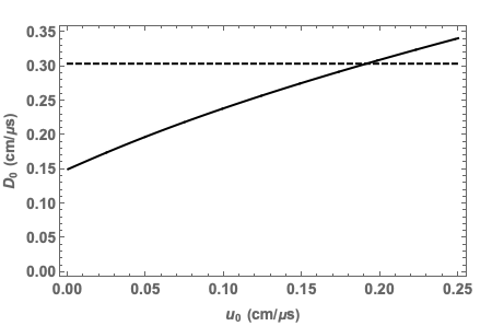
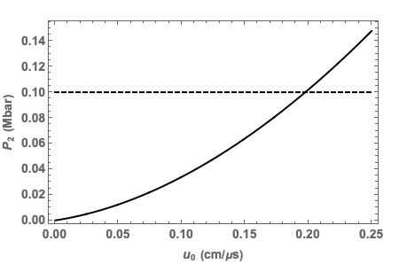

As discussed in Sec. I, a canonical example of an isentropic EOS is the modified Tait EOS given by Eq. (1). The modified Tait form for given by Eq. (1) may be substituted into all of the otherwise arbitrary developments of Sec. V.2 to construct an example solution for the classical Noh problem. As discussed in Sec. V.2, the construction of a 1D planar instantitation of this problem for an isentropic EOS is piecewise constant, and is essentially encapsulated in a solution of Eq. (169). For the modified Tait EOS, this relation becomes
| (170) |
which, given numerical values for the inflow velocity , unshocked density , and the material-dependent constants , , and , can be solved using a root extraction technique.
As an example, Zel’dovich and Raizer Zel’dovich and Raizer 2012 give the following modified Tait parameterization for water:
Assuming throughout the unshocked region, the resulting numerical solution of Eq. (170) is given in Fig. (3) for a range of values. The associated shock speed and shocked fluid pressure, calculated using Eqs. (167) and (1), are depicted in Figs. (3) and (3), respectively. The shocked fluid SIE is calculated using Eqs. (1) and (20), which yield
| (171) |
and is depicted in Fig. 3 for , so that .
Analysis of Eq. (170) shows that a solution is obtained for any . When satisfies this condition, increases from monotonically and without limit with increasing , as depicted in Fig. 3. The shock velocity likewise increases monotonically and without limit with increasing , but as it limits to the sound speed in the unshocked region, which may be calculated using Eqs. (1), (12), (13), and as:
| (172) | |||||
The shocked pressure and shocked SIE likewise increase from zero monotonically and without limit with increasing .
The reason for these behaviors is associated with the modified Tait EOS entropy. Using Eqs. (1), (11), and (12), the entropy in the shocked region may be calculated as
| (173) | |||||
which is explicitly constant for any function of the indicated argument. In particular, the entropy in the shocked region assumes this value for any inflow velocity , and thus is independent of shock strength. Equation (173) thus indicates that given a constant entropy in the shocked region, increasing must always be counterbalanced by increasing .
This behavior is distinct from that encountered in the classical ideal gas Noh problem, which features a maximum shock compression limit independent of . Following from the definition of the ideal gas entropy given by Zel’dovich and Raizer Zel’dovich and Raizer 2012, and the classical 1D planar ideal gas solution disseminated by Ramsey et al. Ramsey et al. 2017, the entropy in the shocked region for this case is given by
| (174) | |||||
where and are interpreted as the constant specific heat capacity at constant volume and constant adiabatic index, respectively. This result clearly depends on and is thus not explicitly constant with respect to that parameter. The difference in behavior of between these two cases is thus clearly revealed to be one consequence of invoking an isentropic EOS assumption in the construction of a classical 1D planar Noh problem.
VI Discussion and Conclusion
Under the assumption of an isentropic EOS of the form given by Eq. (14), the 1D inviscid Euler equations may be collapsed to a set of two coupled, nonlinear PDEs. In this formulation total energy conservation is automatically ensured, as is isentropic flow. A special case of this phenomenon involving explicitly constant entropy is referred to as homentropic flow. Piecewise isentropic or homentropic flows featuring shock waves may also exist in these scenarios, with the shocked and unshocked states connected by an appropriate form of the Rankine-Hugoniot jump conditions.
Moreover, the equations governing any of the aforementioned flows may be subjected to symmetry analysis, in the interest of reducing the PDEs and any ancillary conditions to simpler structures (e.g., ODEs) more easily amenable to either exact or semi-analytical solution. For cases where the included isentropic EOS (encoded in an adibatic bulk modulus ) is left as an arbitrary function of the fluid density , symmetry analysis yields conditional forms the EOS may assume so as to ensure the presence of various symmetries (e.g., scaling transformations). When the isentropic EOS assumes one of these forms, the PDEs governing the associated fluid motion may be reduced to ODEs.
The ODEs obtained via symmetry analysis are likely easier to solve than their PDE counterparts, and thus may be used to construct a variety of exact or semi-analytical solutions with desired properties. Under scaling transformations, one such example is the classical Noh problem featuring a constant velocity inflow directed against a rigid wall (1D planar geometry) or curvilinear origin (1D cylindrical or spherical geometries), giving rise to an outward propagating, constant velocity stagnation shock. For the case of an arbitrary isentropic EOS, the solution of this problem essentially reduces to a transcendental solve in the shocked density , which may then be used to reconstruct the shock trajectory and entire shocked flow field.
VI.1 Recommendations for Future Work
The modified Tait EOS given by Eq. (1) is similar in form to the ideal gas EOS, namely
| (175) |
in that the adibatic bulk moduli calculated from them are only slightly different in form. A potentially fruitful avenue for future work would be to further assess the consequences these differences manifest in solutions of various Noh-like problems, and to investigate the conditions under which one of the result sets can be obtained from the other. Similar efforts could be performed with respect to the recent work of both Deschner et al. Deschner et al. 2018 and Velikovich and Giuliani Velikovich and Giuliani 2018.
Additional natural extensions of this work include (but are not limited to):
- •
Extension of the current results for the modified Tait EOS to other, similar EOS examples with validity in a variety of regimes and contexts. One such example is given by the Birch-Murnaghan EOS, as reported by Birch Birch 1947.
- •
Determination of the conditions for scale-invariance of the homentropic Euler equations in other coordinate systems (e.g., 2D or 3D). Such an analysis should follow easily from that performed in Sec. IV, and can also be connected to various outcomes reported by Ovsiannkov Ovsyannikov 2014 or Holm Holm 1976.
- •
Determination of conditions for the presence of any symmetries (i.e., not limited to scaling transformations) in the homentropic Euler equations, in any coordinate system. For example, in addition to the kinematic scaling () transformation indicated by Eq. (164), the 1D planar instantiation of Eqs. (28) and (30) is for any EOS invariant under time translation, space translation, and Galilean boost transformations (see, for example, Axford Axford 2000). The association with and interplay of these various transformations with canonical solutions remains to be rigorously assessed.
- •
Construction of Sedov, Guderley, or other analogous test problems featuring shock waves in the piecewise homentropic setting, following from the presence of any symmetries.
- •
Construction of additional shock-free solutions (e.g., in the style of Coggeshall Coggeshall 1991 or McHardy et al. McHardy et al. 2019) of the homentropic Euler equations in any coordinate system.
- •
Establishment of the connections between any of the symmetries or associated new solutions described above, and their ideal gas counterparts (if they exist).
Given the wide scope of potential work available in the context of the isentropic Euler equations, this work may serve as a foundation for any future developments and applications along these lines.
VII Acknowledgements
This work was supported by the U.S. Department of Energy (DOE) through the Los Alamos National Laboratory. Los Alamos National Laboratory is operated by Triad National Security, LLC, for the National Nuclear Security Administration of the DOE (contract number 89233218CNA000001). JFG was partially funded through supported by the National Science Foundation (NSF) under Grant No. PHY-1803912. The authors would like to thank E. J. Albright, B. A. Temple, J. D. McHardy, P. J. Jaegers, E. M. Schmidt, J. H. Schmidt, and J. A. Tellez for their valuable insights on these topics. We would also like to thank the two reviewers of this article for their insight.
Appendix A Similarity Variables Substitution into the Euler Equations
The following relations will be useful in the calculation of Eqs. (121) and (122) which are:
| (176) |
and
| (177) |
and
| (178) | |||||
| (179) |
Taking each respective time and space derivative of Eqs. (117) and (119), we have:
| (180) | ||||
| (181) | ||||
| (182) | ||||
| (183) |
We first perform the substitution for Eq. (28), that is
| (184) | |||||
| (185) | |||||
| (186) |
using Eq. (177) we have
| (187) | |||||
| (188) | |||||
| (189) |
which is Eq. (121).
References
- Sedov (2018) L. I. Sedov, Similarity and dimensional methods in mechanics (CRC press, 2018).
- Korobeinikov (1991) V. Korobeinikov, Problems of Point Blast Theory, American Institute of Physics translation series (American Inst. of Physics, 1991).
- Guderley (1942) G. Guderley, Luftfahrtforschung (1942).
- Noh (1987) W. F. Noh, Journal of Computational Physics 72, 78 (1987).
- Menikoff and Plohr (1989) R. Menikoff and B. J. Plohr, Reviews of modern physics 61, 75 (1989).
- Coggeshall (1991) S. V. Coggeshall, Phys. Fluids A: Fluid Dynamics (1989-1993) 3, 757 (1991).
- Ramsey et al. (2012) S. D. Ramsey, J. R. Kamm, and J. H. Bolstad, International Journal of Computational Fluid Dynamics 26, 79 (2012).
- Burnett et al. (2018) S. C. Burnett, K. G. Honnell, S. D. Ramsey, and R. L. Singleton, Journal of Verification, Validation and Uncertainty Quantification 3, 021002 (2018).
- Barenblatt (1996) G. Barenblatt, Scaling, Self-similarity, and Intermediate Asymptotics: Dimensional Analysis and Intermediate Asymptotics, Cambridge Texts in Applied Mathematics (Cambridge University Press, 1996).
- Barenblatt (2003) G. Barenblatt, Scaling, Cambridge Texts in Applied Mathematics (Cambridge University Press, 2003).
- Motz (1979) H. Motz, London and New York, Academic Press, 1979, 299 p. (1979).
- Atzeni and Meyer-ter Vehn (2004) S. Atzeni and J. Meyer-ter Vehn, The physics of inertial fusion: beam plasma interaction, hydrodynamics, hot dense matter, Vol. 125 (OUP Oxford, 2004).
- Meyer-ter Vehn and Schalk (1982) J. Meyer-ter Vehn and C. Schalk, Zeitschrift für Naturforschung A 37, 954 (1982).
- Coggeshall and Axford (1986) S. V. Coggeshall and R. A. Axford, Phys. Fluids (1958-1988) 29, 2398 (1986).
- Coggeshall and Meyer-ter Vehn (1992) S. V. Coggeshall and J. Meyer-ter Vehn, J. Math. Phys. 33, 3585 (1992).
- Birkhoff (2015) G. Birkhoff, Hydrodynamics, Princeton Legacy Library (Princeton University Press, 2015).
- Ovsyannikov (2014) L. Ovsyannikov, Group Analysis of Differential Equations (Elsevier Science, 2014).
- Holm (1976) D. D. Holm, Symmetry breaking in fluid dynamics: Lie group reducible motions for real fluids, Tech. Rep. (Los Alamos Scientific Lab., 1976).
- Hutchens (1990) G. J. Hutchens, Finite–Strength Shock Propagation for Alternative Equations of State, Ph.D. thesis, University of Illinois at Urbana- Champaign (1990).
- Anderson (1990) J. D. Anderson, Modern compressible flow: with historical perspective, Vol. 12 (McGraw-Hill New York, 1990).
- LeVeque (1990) R. J. LeVeque, Numerical Methods for Conservation Laws (Birkhäuser Basel, 1990).
- Zel’dovich and Raizer (2012) Y. Zel’dovich and Y. Raizer, Physics of Shock Waves and High-Temperature Hydrodynamic Phenomena, Dover Books on Physics (Dover Publications, 2012).
- Stanyukovich (2016) K. P. Stanyukovich, Unsteady motion of continuous media (Elsevier, 2016).
- Li (1967) Y.-H. Li, Journal of Geophysical Research 72, 2665 (1967).
- Ridah (1988) S. Ridah, Journal of applied physics 64, 152 (1988).
- Baum et al. (1959) F. Baum, K. Stanyukovich, and B. I. Shekhter, Physics of an Explosion, Tech. Rep. (Army Engineer Research and Development Labs Fort Belvoir VA, 1959).
- Wardlaw and Mair (1998) A. B. Wardlaw and H. U. Mair, Shock and Vibration 5, 89 (1998).
- Cole and Weller (1948) R. H. Cole and R. Weller, Physics Today 1, 35 (1948).
- Akinsete and Lee (1969) V. Akinsete and J. Lee, The Physics of Fluids 12, 428 (1969).
- Hunter (1960) C. Hunter, Journal of Fluid Mechanics 8, 241 (1960).
- Ramsey et al. (2017) S. Ramsey, Z. Boyd, and S. Burnett, Shock Waves 27, 477 (2017).
- Velikovich and Giuliani (2018) A. L. Velikovich and J. L. Giuliani, Phys. Rev. E 98, 013105 (2018).
- Deschner et al. (2018) S. C. Deschner, T. F. Illenseer, and W. J. Duschl, SIAM Journal on Applied Mathematics 78, 80 (2018).
- D. Ramsey and S. Baty (2017) S. D. Ramsey and R. S. Baty, Journal of Mathematical Physics 58, 111506 (2017).
- Harlow and Amsden (1971) F. H. Harlow and A. A. Amsden, Fluid dynamics: a LASL monograph (Mathematical solutions for problems in fluid dynamics), Tech. Rep. LA 4700 (Los Alamos National Laboratory, 1971).
- Mandl (1988) F. Mandl, Statistical Physics, CIBA Foundation Symposium (Wiley, 1988).
- Bowley and Sánchez (1999) R. Bowley and M. Sánchez, Introductory Statistical Mechanics, Oxford science publications (Clarendon Press, 1999).
- Adkins and Adkins (1983) C. Adkins and C. Adkins, Equilibrium Thermodynamics (Cambridge University Press, 1983).
- Landau and Lifshitz (2013) L. Landau and E. Lifshitz, Statistical Physics, v. 5 (Elsevier Science, 2013).
- Zemansky et al. (1966) M. Zemansky, M. Abbott, and H. Van Ness, Basic engineering thermodynamics, International student edition (McGraw-Hill, 1966).
- Axford (2000) R. Axford, Lasers and Particle Beams (2000).
- Harrison and Estabrook (1971) B. K. Harrison and F. B. Estabrook, Journal of Mathematical Physics 12, 653 (1971).
- Lie and Engel (1888) S. Lie and F. Engel, Theorie der Transformationsgruppen, v. 1 (Leipzig: B.G. Teubner, 1888).
- Lie and Engel (1890) S. Lie and F. Engel, Theorie der Transformationsgruppen, v. 2 (Leipzig: B.G. Teubner, 1890).
- Lie and Scheffers (1891) S. Lie and G. Scheffers, Vorlesungen über differentialgleichungen mit bekannten infinitesimalen transformationen (Leipzig: B.G. Teubner, 1891).
- Lie and Scheffers (1893) S. Lie and G. Scheffers, Vorlesungen über continuierliche Gruppen mit geometrischen und anderen Anwendungen (Leipzig: B.G. Teubner, 1893).
- Lie and Engel (1893) S. Lie and F. Engel, Theorie der Transformationsgruppen, v. 3 (Leipzig: B.G. Teubner, 1893).
- Lie (1896) S. Lie, Geometrie der Berührungstransformationen (Leipzig: B.G. Teubner, 1896).
- Bluman and Anco (2008) G. Bluman and S. Anco, Symmetry and Integration Methods for Differential Equations, Applied Mathematical Sciences (Springer New York, 2008).
- Bluman and Kumei (2013) G. Bluman and S. Kumei, Symmetries and Differential Equations, Applied Mathematical Sciences (Springer New York, 2013).
- Olver (1993) P. Olver, Applications of Lie groups to differential equations, Graduate texts in mathematics (Springer-Verlag, 1993).
- Cantwell (2002) B. Cantwell, Introduction to Symmetry Analysis, Cambridge Texts in Applied Mathematics (Cambridge University Press, 2002).
- Edelen (2005) D. Edelen, Applied Exterior Calculus, Dover Books on Mathematics Series (Dover Publications, 2005).
- Suhubi (2013) E. Suhubi, Exterior Analysis: Using Applications of Differential Forms (Elsevier Science, 2013).
- Stephani (1989) H. Stephani, Differential Equations: Their Solution Using Symmetries (Cambridge University Press, 1989).
- Bryant et al. (2013) R. L. Bryant, S.-S. Chern, R. B. Gardner, H. L. Goldschmidt, and P. A. Griffiths, Exterior differential systems, Vol. 18 (Springer Science & Business Media, 2013).
- Bourbaki (1989) N. Bourbaki, Lie Groups and Lie Algebras: Chapters 1-3, Bourbaki, Nicolas: Elements of mathematics (Springer, 1989).
- J. Albright et al. (2018) E. J. Albright, S. D. Ramsey, J. H. Schmidt, and R. S. Baty, Quarterly Journal of Mechanics and Applied Mathematics 71, 25 (2018).
- Courant and Friedrichs (1999) R. Courant and K. Friedrichs, Supersonic Flow and Shock Waves, Applied Mathematical Sciences (Springer New York, 1999).
- Birch (1947) F. Birch, Phys. Rev. 71, 809 (1947).
- McHardy et al. (2019) J. McHardy, E. Albright, S. Ramsey, and J. Schmidt, AIP Advances 9, 085113 (2019).