Ghost-free non-local Gravity Cosmology
Abstract
In this work we shall study ghost-free non-local gravity models. Firstly we shall demonstrate how the ghost degrees of freedom may occur in the non-local gravity models, and accordingly we shall modify appropriately the gravitational action of non-local gravity models in order to eliminate the ghosts. Also we shall investigate how the (anti-)de Sitter and the Minkowski spacetime cosmological solutions may arise in the theory, and we investigate when these solutions are stable. Moreover, we shall examine the inflationary phenomenology of the Jordan frame ghost-free non-local gravity. We shall study two gravity models, the power law gravity model with , and the model, assuming that the slow-roll condition holds true for the Hubble rate during the inflationary era and that the general constant-roll condition holds true for the evolution of the scalar field, which includes the slow-roll case for . As we shall demonstrate, the power-law non-local gravity case can produce a viable inflationary era, compatible with observations, in the constant-roll case, unlike for the model. It is conceivable that the results are model dependent, as in the ordinary vacuum gravity.
I Introduction
Einstein’s final task and idea was to find a unified field theory of everything, a theory in which all the fundamental interactions might be explained in the same framework in a fundamental way. Ever since, theoretical physicists focused in finding the fundamental theory of everything, with the most important theory that emerged being, to our opinion, string theory quantified in its various -theory variants. However, the -theory predictions provide phenomenological results that can be verified at very high energies, making the experimental testing at a pragmatic level, rather an far future or a futile task. Thus the quantization of gravity remains an unsolved problem, and by quantization we mean the whole process of embedding the gravitational field in the already successful field theories that the quantization procedure resulted to experimental verifications of their predictions.
In the process of finding the fundamental theory, however, many physicists realized that it may be possible to discover imprints of the unified theory of everything in the classical physics, by using a up-bottom approach, contrary to the string theory framework which is a bottom-up theory, trying to extract the classical theory, from the fundamental theory itself. Indeed, if one adopts the up-bottom approach, one may seek for effective gravitational theories, that may include terms of the quantum unified theory of everything, accompanying the standard classical theory of the Einstein-Hilbert gravity. The reason for trying to do this is mainly because, although the classical theory of gravity seems to be perfectly describing astrophysical phenomena, at large scales it seems to be lacking of a self-consistent description. Indeed, after the discovery of the accelerating expansion of the Universe Perlmutter:1998np; Riess:1998cb; Spergel:2003cb; Spergel:2006hy; Komatsu:2008hk; Komatsu:2010fb; Tegmark:2003ud; Seljak:2004xh; Eisenstein:2005su; Jain:2003tba, it was realized that a modification of gravity is needed in order to perfectly describe the late-time acceleration era. In this line of research, many modified gravity models have been proposed Nojiri:2017ncd; Nojiri:2010wj; Nojiri:2006ri; Capozziello:2011et; Capozziello:2010zz; delaCruzDombriz:2012xy; Olmo:2011uz, in the context of which the late-time acceleration may be described, or sometimes inflation and dark energy may be described in a unified way within the same theoretical framework Nojiri:2003ft.
One of the most promising modified gravity theories, which also has a direct with an underlying quantum effective theory of gravity, is the non-local gravity, see Refs. Modesto:2017sdr; Belgacem:2017cqo; Koshelev:2016xqb for recent reviews on the subject. This theory was preliminary proposed in Ref. Wetterich:1997bz, however the original version could not take into account cosmological phenomena. A consistent non-local gravity model that took also into account cosmological phenomena, was proposed in Deser:2007jk, and ever since it has been actively investigated Nojiri:2007uq; ArkaniHamed:2002fu; Nojiri:2010pw; Joukovskaya:2007nq; Calcagni:2007ef; Jhingan:2008ym; Capozziello:2008gu; Koshelev:2008ie; Nesseris:2009jf; Deffayet:2009ca; Calcagni:2009dg; Cognola:2009jx; Bronnikov:2009az; Calcagni:2010ab; Vernov:2010ui; Barnaby:2010kx; Dimitrijevic:2019pct; Dialektopoulos:2018iph; Calmet:2018rkj; Bahamonde:2017sdo; Elizalde:2011su; Bamba:2012ky; Deser:2013uya; Deser:2019lmm; Maggiore:2014sia; Chan:2012jj; Koshelev:2016xqb; Zhang:2011uv. In general, the non-local models of gravity, and also of non-local gravity, can be rewritten in a local form by introducing scalar field(s). With the present paper we aim to demonstrate the non-local theories of gravity are compromised by the existence of ghost degrees of freedom, that may result to destabilizing the effective gravitational theory framework of non-local gravity. In addition and more importantly, we aim to propose a direct remedy for the non-local gravity, by providing a ghost-free modification of the non-local gravity theory. We shall thoroughly investigate the cosmological aspects of these theories, and we shall demonstrate that it is possible for these theories to have an exact solution which describe the (anti-)de Sitter or the flat Minkowski spacetime. We also find the conditions for which the solutions become stable. Finally, we shall thoroughly investigate the inflationary phenomenological aspects of the ghost-free non-local gravity theory in the Jordan frame, for a flat cosmological geometry, by assuming a slow or a constant-roll evolution for the scalar field , and the standard slow-roll approximation for the Hubble rate, namely , during the whole inflationary era. We examine two cases of power-law gravity models, a standard power-law , with and , and a gravity model. The reason of discriminating these two cases is mainly a technical simplification that occurs in the case, which enables us to extract more accurate results analytically. For both the cases we present the technical formalism for calculating the slow-roll indexes and the corresponding spectral index of the primordial curvature perturbations and the tensor-to-scalar ratio, and we calculate in detail the Hubble rate as a function of the -foldings number and the free parameters of the theory. As we demonstrate, the power-law gravity can be compatible with the latest (2018) Planck constraints on the inflationary parameters Akrami:2018odb, if the scalar field satisfies the constant-roll evolution, even for small values, however, the produces less appealing phenomenological results.
This paper is organized as follows: In section II we demonstrate how ghosts may occur in non-local gravity theories, while in section III we discuss how we can modify the non-local gravity models action in order to avoid the ghost degrees of freedom. In section IV we study how the (anti-)de Sitter and the Minkowski spacetime solutions can be realized by the ghost free non-local gravity model, and in section V we investigate the phenomenological inflationary predictions of the non-local gravity models, by working in the Jordan frame and in the absence of any matter perfect fluids. We study the ghost-free power-law and non-local and we confront the results with the latest Planck data. Finally, the conclusions follow in the end of the paper.
II Ghost in Non-local Gravity
Before constructing the ghost-free models of non-local gravity, we shall discuss how the ghosts occur in the standard non-local models. We may consider the non-local gravity, whose action is given by,
| (1) |
By introducing two scalar fields and , we may rewrite the action (1) in a local form,
| (2) |
Accordingly, the action can be further cast in the following form,
| (3) |
where and . Furthermore, by introducing additionally two scalar fields and , we may further rewrite the action as follows,
| (4) |
Upon varying the above action with respect to the scalar field , we obtain,
| (5) |
Then we may rewrite the action (4) as follows,
| (6) |
By performing the following scale transformation of the metric,
| (7) |
the action (17) can be obtained in the Einstein frame, and it is equal to,
| (8) |
The above expression indicates that ghost modes occur. First for the simplicity, we consider the case . Then the action (II) is simplified to the following form,
| (9) |
The kinetic terms of the scalar fields , , and are rewritten as follows,
| (10) |
Since the determinant of is given by,
| (11) |
in effect is negative and therefore a ghost mode occurs. Upon varying the action (II) with respect to , we obtain,
| (12) |
which can be solved with respect to as follows,
| (13) |
Then the action (II) can be rewritten as follows,
| (14) |
Thus, the original non-local gravity with action given in Eq. (1) clearly leads to ghost modes. In the next section we propose some modified models of non-local gravity which may alleviate the ghosts.
III Non-local Gravity Models without Ghost
In this section, we construct the models of non-local gravity without ghost modes. As a first example, we consider the following action,
| (15) |
which can be rewritten as follows,
| (16) |
Further, by introducing additionally two scalar field and , we may further rewrite the above action as follows,
| (17) |
Upon variation of the action with respect to , we obtain,
| (18) |
which can be solved with respect to as . Then we can further rewrite the action (17) as follows,
| (19) |
By the scale transformation of the metric,
| (20) |
the action (19) can be rewritten in the Einstein frame, and it is equal to,
| (21) |
As it is clear from the kinetic terms of the scalar fields and , the model has no ghosts as long as .
As an extension of the model (15), we consider the following model,
| (22) |
Then instead of (III) in the Einstein frame, we obtain the following Einstein frame action,
| (23) |
Here is again given by solving (18), . Then if , as clear from the kinetic terms, again, the model has no ghosts.
As another extension of the model (15), we may consider the following action,
| (24) |
which can be rewritten as follows,
| (25) |
Unless , this model has a ghost in general. When , the action (III) takes the following form ,
| (26) |
By introducing which is defined as follows,
| (27) |
we may rewrite the action (26) as follows,
| (28) |
Then we may integrate out of the action, and disregard thereafter, thus the resulting action reads,
| (29) |
The kinetic term indicates that a ghost mode may still occur. In order to avoid this problem, we may deform the model by adding kinetic terms for and as follows,
| (30) |
where and are constants. By the variation of the action with respect to , we obtain,
| (31) |
which can be solved with respect to as follows,
| (32) |
By substituting the above expression of into the action (30), we obtain,
| (33) |
Upon variation of the action (33) with respect to , we obtain,
| (34) |
which we can solve with respect to ,
| (35) |
Then by substituting the above expression into Eq. (33), we obtain the following non-local action,
| (36) |
In order to determine if the model (III) or (30) has a ghost mode or not, we rewrite the action (30) as in Eq. (19), that is,
| (37) |
where is given by solving the equation , again. Then by performing the scale transformation of the metric given in Eq. (20), we obtain the action in the Einstein frame,
| (38) |
Then as long as the following constraints hold true,
| (39) |
no ghost modes occur in the theory.
IV Cosmological Solutions of Ghost-free non-local Gravity Models
In this section we shall investigate whether the ghost free non-local gravity models discussed in the previous section, have solutions some cosmological evolutions of interest. Firstly, let us consider if the model (15) has the Minkowski spacetime or the de Sitter spacetime solution. We start with the form of the action given in Eq. (17). Then in addition to Eq. (18), upon varying the action with respect to , , and , we obtain,
| (40) | ||||
| (41) | ||||
| (42) |
By using the constants and , we now assume,
| (43) |
and we neglect the contribution from the perfect matter fluids hereafter, so . Then by using Eq. (18), also , (40), (41), and Eq. (IV), we obtain,
| (44) |
Then if the following conditions for at ,
| (45) |
are satisfied, we find,
| (46) |
Then if , which satisfies the conditions in (45), is positive, we have the solution describing the de Sitter spacetime. On the other hand, if is negative, we obtain the solution corresponding to the anti-de Sitter spacetime. Furthermore if vanishes, the solution describes the flat Minkowski spacetime. The solution (46) also indicates that,
| (47) |
so this guarantees that no ghost mode occurs upon perturbating around the background. The general form of satisfying the conditions in Eq. (45) is given by,
| (48) |
where is an arbitrary function satisfying . An interesting example is,
| (49) |
Now satisfies the conditions , which has several (anti-)de Sitter solutions corresponding to .
In order to investigate the stability, we consider the potential in (III),
| (50) |
Then the extrema of the potential are found by solving the following equations,
| (51) |
If we assume (46), we find,
| (52) |
Then the (anti-)de Sitter solution in (46) corresponds to the extrema of the potential . Since the following holds true,
| (53) |
for the solution in (46), we find,
| (54) |
Then if the following conditions hold true,
| (55) |
the solution is stable. For example, we assume
| (56) |
where and are constant with appropriate dimensions. Then we find,
| (57) |
and therefore the conditions in Eq. (55) are quantified for the model at hand as follows,
| (58) |
Therefore if , there is a stable de Sitter solution.
V Inflationary Phenomenology of Ghost-free non-Local Gravity Theory
Having discussed the essential features of the ghost-free non-local theories of gravity, in this section we shall explore the inflationary phenomenology of the models in the Jordan frame and in the absence of any perfect matter fluids. Specifically we shall be interested in the model of Eq. (15) or equivalently in the model (16). We quote here the gravitational action for convenience, in the absence of matter fluids, which is,
| (59) |
In the following we introduce the following notation,
| (60) |
and in the following will stand for,
| (61) |
where the prime denotes differentiation with respect to the Ricci scalar. Also, in the following will denote,
| (62) |
Assuming that the background metric is a flat Friedmann-Robertson-Walker (FRW) background with line element,
| (63) |
upon varying the gravitational action (59) with respect to the metric tensor and the scalar field, we obtain the gravitational equation of motion, which for the FRW metric read,
| (64) | ||||
| (65) | ||||
| (66) |
where the “dot” in the above equations denotes differentiation with respect to the cosmic time . For the model (59) the gravitational wave speed is and also the speed of sound is also Hwang:2005hb. Let us work on the equations of motion, and by combining Eqs. (65) and (66) we obtain the following,
| (67) |
The inflationary dynamics for models of the form have been worked out in Ref. Hwang:2005hb. The slow-roll indices are equal to,
| (68) |
where the function appearing above is defined to be,
| (69) |
The scalar perturbations for the theory at hand result to the following spectral index, which is,
| (70) |
and the tensor-to-scalar ratio is in the case at hand,
| (71) |
It is easy to understand that the inflationary phenomenology of the model (59) will highly depend on the gravity model. In the following sections we shall investigate two models of interest, the power law gravity, in which case for general , and a specific case of power-law gravity, the gravity. In both cases we shall assume that the slow-roll condition for the Hubble rate holds true, during the inflationary era, that is,
| (72) |
while the scalar field will be assumed to satisfy the general slow-roll evolution,
| (73) |
However, for convenience and in order to cover simultaneously all the possible dynamical evolutions for the scalar field, we shall assume that the scalar field evolves as,
| (74) |
so when , the scalar field obeys the constant-roll evolution rules Martin:2012pe; Nojiri:2017qvx, and when the scalar field evolves in the standard slow-roll way. Note that the slow-roll conditions for the Hubble rate (72) do not affect directly, or are not related to the evolution of the scalar field. However, the two evolutions are related once the equations of motion are used, at a fundamental level though, the evolution conditions are unrelated.
V.1 General non-local Ghost Free Power-law Gravity Inflationary Phenomenology
Let us firstly consider the case that the gravity appearing in the action of Eq. (59) has the general power-law form,
| (75) |
with being any number except for , which will be discussed in the next subsection, and being a dimensionful parameter of the theory. In this case, by using the slow-roll condition for the scalar field (74), the equation of motion (66) for the scalar field yields,
| (76) |
and due to the fact that the Ricci scalar for the FRW metric is , in conjunction with the slow-roll condition (72), the Ricci scalar during the inflationary era is , so we may algebraically solve the equation (76) with respect to and we obtain,
| (77) |
where stands for,
| (78) |
The slow-roll conditions for the Hubble rate can help us to obtain approximate relations for the evolution of , expressed in terms of the Hubble rate. In this way, we may solve the equations of motion in order to have an approximate expression for the Hubble rate, and eventually discover the phenomenological implications of the power-law model at hand. Unless we follow this research line, the solution of the cosmological equations cannot be obtained in an analytic way, and the task finding the inflationary dynamics is impossible.
For the model at hand we have,
| (79) |
and due to the fact that during the inflationary era, the second term overwhelms the evolution (recall ), we have approximately,
| (80) |
Then, the first Friedman equation, namely Eq. (64) for the model at hand reads,
| (81) |
The last term is subdominant, therefore at leading order it can be omitted. Therefore, the resulting equation can be rewritten as,
| (82) |
By using the approximation , we finally obtain,
| (83) |
where is,
| (84) |
Having Eqs. (83) and (77) at hand, we can easily express the slow-roll indices (68) in terms of the Hubble rate, always having in mind the slow-roll conditions (72), so we obtain the following simplified solutions,
| (85) |
As it is obvious, the slow-roll indices and can be expressed as a function of the slow-roll index , so these two can be further written as,
| (86) |
Eventually, what remains is to find the approximate cosmological evolution generated by the non-local power-law gravity model at hand, in the slow-roll approximation. So by substituting the evolution for and from Eqs. (83) and (77) in the differential equation (67), we may obtain a differential equation for the Hubble rate, and by solving it, we can find the cosmological evolution during the inflationary era for the model at hand. So at leading order, in view of Eqs. (83) and (77), the differential equation (67) at leading order reads,
| (87) |
so by using the approximation which holds true during the inflationary era, and by keeping the dominant terms, we finally obtain the following approximate analytic solution,
| (88) |
where and are defined in Eqs. (84) and (98). Note that the above evolution does not necessarily describe an inflationary evolution, but as we shall demonstrate, for the values of the parameters that guarantee the phenomenological viability of the model, the evolution is as expected an inflationary evolution.
Let us proceed to investigate the phenomenological viability of the model. The slow-roll indices are easily obtained since these are expressed in terms of the slow-roll index , which for the Hubble rate (88) reads,
| (89) |
and accordingly, the observational indices and appearing in Eqs. (70) and (71) can easily be calculated and expressed in terms of the free parameters of the theory. We shall not quote here the resulting expression for the spectral index, since it is too lengthy, but the tensor-scalar-ratio has a particular simple form which is,
| (90) |
Also it is notable that the resulting expression of the spectral index is -independent, and the same applies for the tensor-to-scalar ratio (90). At this point we can check the viability of the model easily by using specific values for the free parameters. For simplicity we shall use the reduced Planck physical units system in which .
A thorough investigation of the free parameters space shows that the viability of the model comes relatively easy in this power-law model, however, only in the constant-roll case evolution. Indeed, by choosing for example and in reduced Planck units, we have,
| (91) |
which are compatible with the latest (2018) Planck constraints Akrami:2018odb on the spectral index and the tensor-to-scalar ratio, which are,
| (92) |
It can be shown that the simultaneous compatibility of the spectral index and the tensor-to-scalar ratio with the Planck data occurs for a wide range of values of the free parameters and . This can be seen in Fig. 1 where we present the plots of the spectral index (left) and of the tensor-to-scalar ratio (right) in the ranges and .
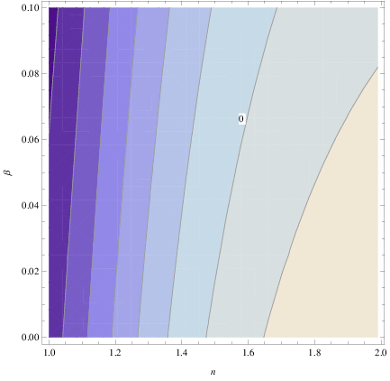
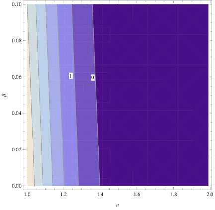
It would be expected that the viability in the constant-roll case comes for a wider range of values of , but on the contrary, only small values of () guarantee the viability of the model. Finally, let us show explicitly that the evolution given in Eq. (88) indeed describes an inflationary evolution for the allowed values of the parameters. The Hubble rate (88) corresponds to the scale factor,
| (93) |
and by choosing and in reduced Planck units, for which values the viability of the model is ensured, we have,
| (94) |
so and we definitely have an inflationary solution. This result occurs for a wide range of parameter values and an inflationary solution is guaranteed for values of and for which .
V.2 Non-local Ghost-free Gravity Inflationary Phenomenology
Having discussed the non-local power-law gravity model, in this section we shall investigate the gravity case. We discriminate it from the power-law gravity case, because in the case, the gravitational equations are more easy to study, and thus more accurate results may be obtained. This discrimination between the two cases can be found in the context of pure gravity, see the discussion in Ref. Odintsov:2019evb. In the case, the gravity function appearing in the action of Eq. (59) has the form,
| (95) |
assuming that the constant-roll conditions hold true for the scalar field (74) and the slow-roll condition holds true for the Hubble rate (72), we have for the scalar field equation of motion,
| (96) |
and since the Ricci scalar during the inflationary era is , so solve the equation (96) with respect to and we obtain,
| (97) |
where stands for,
| (98) |
Following the method of the previous section, we substitute from Eq. (97) into equation (64), and using the fact that during inflation,
| (99) |
we easily obtain as a function of the Hubble rate, which is,
| (100) |
where in this case is,
| (101) |
Having Eqs. (100) and (97) at hand, we can easily express the slow-roll indices (68) in terms of the Hubble rate, as follows, solutions,
| (102) |
As it is obvious, the slow-roll indices and can be expressed in this case too as a function of the slow-roll index , so we rewrite these two as follows,
| (103) |
As in the previous section, what now remains is to find the approximate cosmological evolution realized by the non-local gravity, so by substituting the evolution for and from Eqs. (100) and (97) in the differential equation (67), we obtain the following differential equation at leading order,
| (104) |
which is obviously different from the one corresponding to the power-law case appearing in Eq. (). Note that in Eq. (104) is equal to,
| (105) |
The differential equation (104) has the following analytic solution,
| (106) |
where is an integration constant. Obviously the solution (106) is different from the one corresponding to the power-law case of the previous section, namely Eq. (88). The solution (106) is particularly interesting, since it describes a non-singular cosmology, for , or a cosmology which leads to a future Type III future singularity if , see Ref. Nojiri:2005sx for the classification of future singularities. In this paper we shall consider the phenomenology of the cosmological evolution (106) in the context of non-local gravity, but it is surely worth investigating from which pure gravity this cosmological evolution can be generated, and if it is viable, but we defer this task to a future work. Focusing on the non-local model at hand, by combining Eqs. (103) and (106), also by solving the equation and by expressing the horizon crossing time, as a function of the -foldings number and the final time , we obtain the analytic form of the slow-roll indices in terms of the free parameters of the model,
| (107) |
which are evaluated at the time instance of the first horizon crossing. Accordingly the spectral index of the primordial scalar curvature perturbations reads,
| (108) |
while the tensor-to-scalar ratio reads,
| (109) |
so it is dependent. A direct substitution in the tensor-to-scalar ratio results to which in turn indicates that the slow-roll case of the non-local gravity model yields phenomenologically non-viable results. Thus we concentrate on the constant-roll case with . In fact, the 2018 Planck constraint on the tensor-to-scalar ratio, namely can be satisfied when , so the viability for this model comes for abnormally large values of . For example, if we work in reduced Planck units with , if we choose , and , we have,
| (110) |
which are compatible with the latest (2018) Planck constraints (92). Although the model is viable in the constant-roll case, the non-local gravity model is deemed rather physically unappealing, due to the abnormally large values of the parameter . This result indicates that the non-local gravity models are viable in general, but the viability is model dependent, like in the ordinary gravity models of course.
As we already discussed, the cosmology (106) is generated by the non-local model, however, it would be interesting to investigate which pure gravity can generate this cosmological evolution, and whether this cosmological evolution can be phenomenologically viable. We defer this task to a future work.
VI Conclusions
In this paper we studied ghost-free non-local gravity models. Our first aim was to demonstrate how ghost degrees of freedom can arise in these theories, so after having shown that, we investigated how it is possible to obtain ghost-free non-local gravity theories. By appropriately modifying the gravitational action of non-local gravity theories, we demonstrated that ghost-free theories may be obtained, and we extracted the conditions which must be fulfilled in order to have ghost-free theories. Also we investigated whether (anti-)de Sitter and Minkowski spacetime cosmological solutions may arise in the theory, and we examined the stability conditions for these theories. Moreover we studied the inflationary phenomenology of the Jordan frame ghost-free non-local gravity. We presented in detail the essential features of the inflationary dynamics of the model, quantified in the slow-roll indices and the corresponding spectral index of the primordial curvature perturbations and the tensor-to-scalar ratio. Then we focused on two gravity models, the power law gravity model with , and the model. The reason for discriminating among the two power-law models is that in the case of the model, the gravitational equations of motion are greatly simplified and more accurate analytic results may be obtained. In both cases we assumed that the slow-roll condition on the Hubble rate holds true during the inflationary era, namely and also that the scalar field obeys the general constant-roll condition , which is reduced to the slow-roll case when . As we have shown, the power-law non-local gravity case produces a viable inflationary era, compatible with the latest (2018) Planck data, when the constant-roll condition holds true for the scalar field even for small values. On the other hand, the non-local gravity model was deemed not appealing, since it generates a viable inflationary phenomenology compatible with the observational data only when takes values larger than , which is rather not appealing, if not unphysical. The results are of course model-dependent and a better choice of the gravity can in principle enhance the viability of the model even in the slow-roll evolution case for the scalar field, but we chose the simplest examples in order to just demonstrate the argument.
An interesting feature we found is the form of the Hubble rate during the inflationary era corresponding to the non-local gravity model. It is interesting to investigate from which pure vacuum gravity this cosmological evolution is realized, and whether this evolution is a viable cosmological evolution. Work is in progress towards this research line.
Acknowledgments
This work is supported by MINECO (Spain), FIS2016-76363-P, and by project 2017 SGR247 (AGAUR, Catalonia) (S.D.O). This work is also supported by MEXT KAKENHI Grant-in-Aid for Scientific Research on Innovative Areas “Cosmic Acceleration” No. 15H05890 (S.N.) and the JSPS Grant-in-Aid for Scientific Research (C) No. 18K03615 (S.N.).
References
- (1) S. Perlmutter et al. [Supernova Cosmology Project Collaboration], Astrophys. J. 517 (1999) 565 doi:10.1086/307221 [astro-ph/9812133].
- (2) A. G. Riess et al. [Supernova Search Team], Astron. J. 116 (1998) 1009 doi:10.1086/300499 [astro-ph/9805201].
- (3) D. N. Spergel et al. [WMAP Collaboration], Astrophys. J. Suppl. 148 (2003) 175 doi:10.1086/377226 [astro-ph/0302209].
- (4) D. N. Spergel et al. [WMAP Collaboration], Astrophys. J. Suppl. 170 (2007) 377 doi:10.1086/513700 [astro-ph/0603449].
- (5) E. Komatsu et al. [WMAP Collaboration], Astrophys. J. Suppl. 180 (2009) 330 doi:10.1088/0067-0049/180/2/330 [arXiv:0803.0547 [astro-ph]].
- (6) E. Komatsu et al. [WMAP Collaboration], Astrophys. J. Suppl. 192 (2011) 18 doi:10.1088/0067-0049/192/2/18 [arXiv:1001.4538 [astro-ph.CO]].
- (7) M. Tegmark et al. [SDSS Collaboration], Phys. Rev. D 69 (2004) 103501 doi:10.1103/PhysRevD.69.103501 [astro-ph/0310723].
- (8) U. Seljak et al. [SDSS Collaboration], Phys. Rev. D 71 (2005) 103515 doi:10.1103/PhysRevD.71.103515 [astro-ph/0407372].
- (9) D. J. Eisenstein et al. [SDSS Collaboration], Astrophys. J. 633 (2005) 560 doi:10.1086/466512 [astro-ph/0501171].
- (10) B. Jain and A. Taylor, Phys. Rev. Lett. 91 (2003) 141302 doi:10.1103/PhysRevLett.91.141302 [astro-ph/0306046].
- (11) S. Nojiri, S. D. Odintsov and V. K. Oikonomou, Phys. Rept. 692 (2017) 1 doi:10.1016/j.physrep.2017.06.001 [arXiv:1705.11098 [gr-qc]].
- (12) S. Nojiri and S. D. Odintsov, Phys. Rept. 505 (2011) 59 doi:10.1016/j.physrep.2011.04.001 [arXiv:1011.0544 [gr-qc]].
- (13) S. Nojiri and S. D. Odintsov, eConf C 0602061 (2006) 06 [Int. J. Geom. Meth. Mod. Phys. 4 (2007) 115] doi:10.1142/S0219887807001928 [hep-th/0601213].
- (14) S. Capozziello and M. De Laurentis, Phys. Rept. 509 (2011) 167 doi:10.1016/j.physrep.2011.09.003 [arXiv:1108.6266 [gr-qc]].
- (15) V. Faraoni and S. Capozziello, Fundam. Theor. Phys. 170 (2010). doi:10.1007/978-94-007-0165-6
- (16) A. de la Cruz-Dombriz and D. Saez-Gomez, Entropy 14 (2012) 1717 doi:10.3390/e14091717 [arXiv:1207.2663 [gr-qc]].
- (17) G. J. Olmo, Int. J. Mod. Phys. D 20 (2011) 413 doi:10.1142/S0218271811018925 [arXiv:1101.3864 [gr-qc]].
- (18) S. Nojiri and S. D. Odintsov, Phys. Rev. D 68 (2003) 123512 doi:10.1103/PhysRevD.68.123512 [hep-th/0307288].
- (19) L. Modesto and L. Rachwal, Int. J. Mod. Phys. D 26 (2017) no.11, 1730020. doi:10.1142/S0218271817300208
- (20) E. Belgacem, Y. Dirian, S. Foffa and M. Maggiore, JCAP 1803 (2018) 002 doi:10.1088/1475-7516/2018/03/002 [arXiv:1712.07066 [hep-th]].
- (21) A. S. Koshelev, L. Modesto, L. Rachwal and A. A. Starobinsky, JHEP 1611 (2016) 067 doi:10.1007/JHEP11(2016)067 [arXiv:1604.03127 [hep-th]].
- (22) C. Wetterich, Gen. Rel. Grav. 30 (1998) 159 doi:10.1023/A:1018837319976 [gr-qc/9704052].
- (23) S. Deser and R. P. Woodard, Phys. Rev. Lett. 99 (2007) 111301 doi:10.1103/PhysRevLett.99.111301 [arXiv:0706.2151 [astro-ph]].
- (24) S. Nojiri and S. D. Odintsov, Phys. Lett. B 659 (2008) 821 doi:10.1016/j.physletb.2007.12.001 [arXiv:0708.0924 [hep-th]].
- (25) N. Arkani-Hamed, S. Dimopoulos, G. Dvali and G. Gabadadze, hep-th/0209227.
- (26) S. Nojiri, S. D. Odintsov, M. Sasaki and Y. l. Zhang, Phys. Lett. B 696 (2011) 278 doi:10.1016/j.physletb.2010.12.035 [arXiv:1010.5375 [gr-qc]].
- (27) L. Joukovskaya, Phys. Rev. D 76 (2007) 105007 doi:10.1103/PhysRevD.76.105007 [arXiv:0707.1545 [hep-th]].
- (28) G. Calcagni, M. Montobbio and G. Nardelli, Phys. Lett. B 662 (2008) 285 doi:10.1016/j.physletb.2008.03.024 [arXiv:0712.2237 [hep-th]].
- (29) S. Jhingan, S. Nojiri, S. D. Odintsov, M. Sami, I. Thongkool and S. Zerbini, Phys. Lett. B 663 (2008) 424 doi:10.1016/j.physletb.2008.04.054 [arXiv:0803.2613 [hep-th]].
- (30) S. Capozziello, E. Elizalde, S. Nojiri and S. D. Odintsov, Phys. Lett. B 671 (2009) 193 doi:10.1016/j.physletb.2008.11.060 [arXiv:0809.1535 [hep-th]].
- (31) N. A. Koshelev, Grav. Cosmol. 15 (2009) 220 doi:10.1134/S0202289309030049 [arXiv:0809.4927 [gr-qc]].
- (32) S. Nesseris and A. Mazumdar, Phys. Rev. D 79 (2009) 104006 doi:10.1103/PhysRevD.79.104006 [arXiv:0902.1185 [astro-ph.CO]].
- (33) C. Deffayet and R. P. Woodard, JCAP 0908 (2009) 023 doi:10.1088/1475-7516/2009/08/023 [arXiv:0904.0961 [gr-qc]].
- (34) G. Calcagni and G. Nardelli, Int. J. Mod. Phys. D 19 (2010) 329 doi:10.1142/S0218271810016440 [arXiv:0904.4245 [hep-th]].
- (35) G. Cognola, E. Elizalde, S. Nojiri, S. D. Odintsov and S. Zerbini, Eur. Phys. J. C 64 (2009) 483 doi:10.1140/epjc/s10052-009-1154-4 [arXiv:0905.0543 [gr-qc]].
- (36) K. A. Bronnikov and E. Elizalde, Phys. Rev. D 81 (2010) 044032 doi:10.1103/PhysRevD.81.044032 [arXiv:0910.3929 [hep-th]].
- (37) G. Calcagni and G. Nardelli, Phys. Rev. D 82 (2010) 123518 doi:10.1103/PhysRevD.82.123518 [arXiv:1004.5144 [hep-th]].
- (38) S. Y. Vernov, Phys. Part. Nucl. Lett. 8 (2011) 310 doi:10.1134/S1547477111030228 [arXiv:1005.0372 [astro-ph.CO]].
- (39) N. Barnaby, Nucl. Phys. B 845 (2011) 1 doi:10.1016/j.nuclphysb.2010.11.016 [arXiv:1005.2945 [hep-th]].
- (40) I. Dimitrijevic, B. Dragovich, A. S. Koshelev, Z. Rakic and J. Stankovic, doi:10.1016/j.physletb.2019.134848 arXiv:1906.07560 [gr-qc].
- (41) K. F. Dialektopoulos, D. Borka, S. Capozziello, V. Borka Jovanovic and P. Jovanovic, Phys. Rev. D 99 (2019) no.4, 044053 doi:10.1103/PhysRevD.99.044053 [arXiv:1812.09289 [astro-ph.GA]].
- (42) X. Calmet, B. K. El-Menoufi, B. Latosh and S. Mohapatra, Eur. Phys. J. C 78 (2018) no.9, 780 doi:10.1140/epjc/s10052-018-6265-3 [arXiv:1809.07606 [hep-th]]
- (43) S. Bahamonde, S. Capozziello and K. F. Dialektopoulos, Eur. Phys. J. C 77 (2017) no.11, 722 doi:10.1140/epjc/s10052-017-5283-x [arXiv:1708.06310 [gr-qc]].
- (44) E. Elizalde, E. O. Pozdeeva and S. Y. Vernov, Phys. Rev. D 85 (2012) 044002 doi:10.1103/PhysRevD.85.044002 [arXiv:1110.5806 [astro-ph.CO]].
- (45) K. Bamba, S. Nojiri, S. D. Odintsov and M. Sasaki, Gen. Rel. Grav. 44 (2012) 1321 doi:10.1007/s10714-012-1342-7 [arXiv:1104.2692 [hep-th]].
- (46) S. Deser and R. P. Woodard, JCAP 1311 (2013) 036 doi:10.1088/1475-7516/2013/11/036 [arXiv:1307.6639 [astro-ph.CO]].
- (47) S. Deser and R. P. Woodard, JCAP 1906, 034 (2019) doi:10.1088/1475-7516/2019/06/034 [arXiv:1902.08075 [gr-qc]].
- (48) M. Maggiore and M. Mancarella, Phys. Rev. D 90 (2014) no.2, 023005 doi:10.1103/PhysRevD.90.023005 [arXiv:1402.0448 [hep-th]].
- (49) K. C. Chan, R. Scoccimarro and R. K. Sheth, Phys. Rev. D 85 (2012) 083509 doi:10.1103/PhysRevD.85.083509 [arXiv:1201.3614 [astro-ph.CO]].
- (50) Y. l. Zhang and M. Sasaki, Int. J. Mod. Phys. D 21 (2012) 1250006 doi:10.1142/S021827181250006X [arXiv:1108.2112 [gr-qc]].
- (51) Y. Akrami et al. [Planck Collaboration], arXiv:1807.06211 [astro-ph.CO].
- (52) J. c. Hwang and H. Noh, Phys. Rev. D 71 (2005) 063536 doi:10.1103/PhysRevD.71.063536 [gr-qc/0412126].
- (53) J. Martin, H. Motohashi and T. Suyama, Phys. Rev. D 87 (2013) no.2, 023514 doi:10.1103/PhysRevD.87.023514 [arXiv:1211.0083 [astro-ph.CO]].
- (54) S. Nojiri, S. D. Odintsov and V. K. Oikonomou, Class. Quant. Grav. 34 (2017) no.24, 245012 doi:10.1088/1361-6382/aa92a4 [arXiv:1704.05945 [gr-qc]].
- (55) S. D. Odintsov and V. K. Oikonomou, Phys. Rev. D 99 (2019) no.10, 104070 doi:10.1103/PhysRevD.99.104070 [arXiv:1905.03496 [gr-qc]].
- (56) S. Nojiri, S. D. Odintsov and S. Tsujikawa, Phys. Rev. D 71 (2005) 063004 doi:10.1103/PhysRevD.71.063004 [hep-th/0501025].