跳到论文正文
W Papers独立论文阅读器 arXiv:1911.07138 论文正文 计算阅读时间 · 0%
引用这篇论文根据当前论文元数据生成,正式投稿前建议核对。


License: arXiv.org perpetual non-exclusive license
arXiv:1911.07138v3 [cond-mat.str-el] 23 Mar 2020

Theory of Two-Dimensional Nonlinear Spectroscopy for the Kitaev Spin Liquid

Wonjune Choi Affiliation: Department of Physics, University of Toronto, Toronto, Ontario M5S 1A7, Canada    Ki Hoon Lee Affiliation: Center for Correlated Electron Systems, Institute for Basic Science (IBS), Seoul National University, Seoul 08826, Korea Affiliation: Department of Physics and Astronomy, Seoul National University, Seoul 08826, Korea    Yong Baek Kim Affiliation: Department of Physics, University of Toronto, Toronto, Ontario M5S 1A7, Canada
Abstract

Unambiguous identification of fractionalized excitations in quantum spin liquids has been a long- standing issue in correlated topological phases. Conventional spectroscopic probes, such as the dynamical spin structure factor, can only detect composites of fractionalized excitations, leading to a broad continuum in energy. Lacking a clear signature in conventional probes has been the biggest obstacle in the field. In this work, we theoretically investigate what kinds of distinctive signatures of fractionalized excitations can be probed in two-dimensional nonlinear spectroscopy by considering the exactly solvable Kitaev spin liquids. We demonstrate the existence of a number of salient features of the Majorana fermions and fluxes in two-dimensional nonlinear spectroscopy, which provide crucial information about such excitations.

Refer to caption
Figure 1: Two-dimensional Fourier spectrum of the third-order susceptibilities (a) χz​z​z(3),z​(ω2,ω1,0)\chi^{(3),z}_{zzz}(\omega_{2},\omega_{1},0) and (b) χz​z​z(3),z​(ω2,0,ω1)\chi^{(3),z}_{zzz}(\omega_{2},0,\omega_{1}) show the sharp vertical line signals at the two-flux gap, ω1=E2−E0\omega_{1}=E_{2}-E_{0}. (b) χz​z​z(3),z​(ω2,0,ω1)\chi^{(3),z}_{zzz}(\omega_{2},0,\omega_{1}) has one sharp diagonal signal for the Majorana fermions from Rz​z​z(3),zR^{(3),z}_{zzz} and two diagonal signals from Rz​z​z(1),zR^{(1),z}_{zzz} and Rz​z​z(4),zR^{(4),z}_{zzz}. The two diagonal signals from Rz​z​z(1),zR^{(1),z}_{zzz} and Rz​z​z(3),zR^{(3),z}_{zzz} are extrapolated to finite ω2\omega_{2} intercept at the four-flux gap ±(E4−E0)\pm(E_{4}-E_{0}), which hints at the four-flux intermediate states of the perturbative processes.

Quantum spin liquids (QSLs) are prominent examples of correlated topological paramagnets that may arise due to frustrating spin interactions in Mott insulators Balents 2010; Savary and Balents 2017. The long-range quantum entanglement and ground state degeneracy, which comprises the quantum order, differentiate QSLs from trivial paramagnets and symmetry-broken phases Wen 2002. Important manifestations of the quantum order are the emergent gauge fields and quasiparticles carrying fractional quantum numbers Kitaev 2003. Since the quantum entanglement is not directly observable, measuring these fractionalized excitations would be an important experimental footstep to identify quantum spin liquids. One of the most powerful probes in magnetism, the dynamical spin structure factor measured in inelastic neutron scattering, however, shows only a broad continuum as the spin-flip involves a multitude of fractionalized excitations. The absence of sharp signatures has hampered the progress in the discovery of quantum spin liquids.

In this Letter, we consider two-dimensional nonlinear spectroscopy as a tool to detect distinctive signatures of fractionalized quasiparticles in quantum spin liquids. The current work is motivated by a previous work that shows how the domain wall excitations in the transverse field Ising model can clearly be detected in two-dimensional THz spectroscopy Wan and Armitage 2019. Here we consider the exactly solvable Kitaev spin liquids on the honeycomb lattice Kitaev 2006 and investigate the signatures of Majorana fermions and fluxes in two-dimensional spectroscopy. We consider two magnetic-field pulses separated by time τ1\tau_{1} and measuring the nonlinear part of the induced transient magnetization at later time τ2+τ1\tau_{2}+\tau_{1}. The two-dimensional spectroscopy is represented by two frequencies corresponding to τ1\tau_{1} and τ2\tau_{2}. The response consists of nonlinear susceptibilities, some of which correspond to the out-of-time-order correlators of the magnetization Mukamel 1995. We show that the third order nonlinear susceptibilities can give rise to clear signatures of the Majorana fermions and fluxes in the Kitaev spin liquids. We explain how one could obtain important information about such excitations from the output of the two-dimensional spectroscopy. Our main results are shown in Fig. 1.

Model.—On a honeycomb lattice with 2​N2N number of sites, we consider Kitaev’s spin-12\frac{1}{2} Hamiltonian with the isotropic strength of the bond-directional interactions Kitaev 2006,

H^=−∑x​-bondσ^xjσ^xk−∑y​-bondσ^yjσ^yk−∑z​-bondσ^zjσ^zk,\hat{H}=-\sum_{x\text{-bond}}\hat{\sigma}^{x}_{j}\hat{\sigma}^{x}_{k}-\sum_{y\text{-bond}}\hat{\sigma}^{y}_{j}\hat{\sigma}^{y}_{k}-\sum_{z\text{-bond}}\hat{\sigma}^{z}_{j}\hat{\sigma}^{z}_{k}, (1)

where σ^jx,y,z\hat{\sigma}^{x,y,z}_{j} are the Pauli operators at site jj. The model has a constant of motion W^p=σ^1x​σ^2y​σ^3z​σ^4x​σ^5y​σ^6z=±1\hat{W}_{p}=\hat{\sigma}_{1}^{x}\hat{\sigma}_{2}^{y}\hat{\sigma}_{3}^{z}\hat{\sigma}_{4}^{x}\hat{\sigma}_{5}^{y}\hat{\sigma}_{6}^{z}=\pm 1 for each hexagonal plaquette pp, and we say there is a static ℤ2\mathbb{Z}_{2} flux at pp when W^p=−1\hat{W}_{p}=-1.

By representing the Pauli operators in terms of Majorana fermions, σ^jα≐i​bjα​cj\hat{\sigma}_{j}^{\alpha}\doteq ib_{j}^{\alpha}c_{j}, we can rewrite the model as ℤ2\mathbb{Z}_{2} gauge theory coupled to itinerant Majorana fermions,

H~=∑α​-bondi​u^j​kα​cj​ck⇒H~u=∑pεp​(ap†​ap−12),\widetilde{H}=\sum_{\alpha\text{-bond}}i\hat{u}^{\alpha}_{jk}c_{j}c_{k}\Rightarrow\widetilde{H}_{u}=\sum_{p}\varepsilon_{p}\left(a^{\dagger}_{p}a_{p}-\frac{1}{2}\right), (2)

where apa_{p} represents the normal-mode complex fermions. The model is exactly solvable because the emergent ℤ2\mathbb{Z}_{2} gauge fields u^j​kα≡i​bjα​bkα\hat{u}_{jk}^{\alpha}\equiv ib_{j}^{\alpha}b_{k}^{\alpha} commute with H~\widetilde{H} and themselves so that the Hilbert space is factorized into the gauge (flux) sector and the matter fermion sector, ℋ=ℋF⊗ℋM\mathcal{H}=\mathcal{H}_{F}\otimes\mathcal{H}_{M}. Hence, for a given gauge configuration |F⟩=|{uj​kα=±1}⟩∈ℋF|F\rangle=|\{u_{jk}^{\alpha}=\pm 1\}\rangle\in\mathcal{H}_{F}, H~\widetilde{H} is reduced to a quadratic Hamiltonian H~u\widetilde{H}_{u} for the itinerant Majorana fermion cc, whose eigenstates |M⟩|M\rangle span the matter fermion sector ℋM\mathcal{H}_{M}.

Two-dimensional spectroscopy.—To probe the fractionalized excitations of the Kitaev spin liquid, we consider a nonlinear magnetic resonance spectroscopy with two linearly polarized, spatially uniform pulses separated by time τ1\tau_{1},

𝐁⁡(t)=B0​z^​δ​(t)+B1​z^​δ​(t−τ1),\displaystyle\mathbf{B}(t)=B_{0}\hat{z}\delta(t)+B_{1}\hat{z}\delta(t-\tau_{1}), (3)

where the two incident pulses B0B_{0} and B1B_{1} arrive at the system at t=0t=0 and t=τ1t=\tau_{1}, respectively Wan and Armitage 2019; Lu et al. 2017. For simplicity, here we consider the case where the incident pulses are all polarized along the z^\hat{z} direction. These magnetic fields linearly couple to the local moments H^tot​(t)=H^−∑jBz​(t)​σ^jz=H^−Bz​(t)​M^z\hat{H}_{\mathrm{tot}}(t)=\hat{H}-\sum_{j}B^{z}(t)\hat{\sigma}^{z}_{j}=\hat{H}-B^{z}(t)\hat{M}^{z} and induce finite transient magnetization M^01z​(t)\hat{M}^{z}_{01}(t) measured at later time t=τ2+τ1t=\tau_{2}+\tau_{1}. To discard the leading contributions from the linear response, two subsequent experiments measure M^0z​(t)\hat{M}^{z}_{0}(t) and M^1z​(t)\hat{M}^{z}_{1}(t) due to only a single pulse B0B_{0} or B1B_{1}, respectively. The nonlinear induced magnetization defined as M^NLz​(t)=M^01z​(t)−M^0z​(t)−M^1z​(t)\hat{M}^{z}_{\mathrm{NL}}(t)=\hat{M}^{z}_{01}(t)-\hat{M}^{z}_{0}(t)-\hat{M}^{z}_{1}(t) at later time t=τ1+τ2t=\tau_{1}+\tau_{2} depends only on the nonlinear dynamical responses Wan and Armitage 2019,

MNLz\displaystyle M^{z}_{\text{NL}} (τ1+τ2)/2​N=χz​z(2),z​(τ2,τ1)​B1z​B0z\displaystyle(\tau_{1}+\tau_{2})/2N=\chi^{(2),z}_{zz}(\tau_{2},\tau_{1})B_{1}^{z}B_{0}^{z} (4)
+χz​z​z(3),z​(τ2,τ1,0)​B1z​B0z​B0z\displaystyle+\chi^{(3),z}_{zzz}(\tau_{2},\tau_{1},0)B_{1}^{z}B_{0}^{z}B_{0}^{z} (5)
+χz​z​z(3),z​(τ2,0,τ1)​B1z​B1z​B0z+𝒪⁡(B4),\displaystyle+\chi^{(3),z}_{zzz}(\tau_{2},0,\tau_{1})B_{1}^{z}B_{1}^{z}B_{0}^{z}+\mathcal{O}(B^{4}), (6)

where time-dependent perturbation theory gives the nnth-order susceptibility Mukamel 1995 (we choose the unit ℏ=1\hbar=1),

χ(n),zz,…,z(τn,…,τ1)=in2​N⟨[[…[M^z(τn+…+τ1),M^z(τn−1+…+τ1)],…],M^z(0)]⟩.\chi^{(n),z}_{z,...,z}(\tau_{n},...,\tau_{1})=\frac{i^{n}}{2N}\langle[[...[\hat{M}^{z}(\tau_{n}+...+\tau_{1}),\\ \hat{M}^{z}(\tau_{n-1}+...+\tau_{1})],...],\hat{M}^{z}(0)]\rangle. (7)

Second-order susceptibility.—The second-order susceptibility χz​z(2),z​(τ2,τ1)\chi^{(2),z}_{zz}(\tau_{2},\tau_{1}) can be calculated from the three-point correlation functions Mukamel 1995,

χz​z(2),z​(τ2,τ1)\displaystyle\chi^{(2),z}_{zz}(\tau_{2},\tau_{1}) =i2N​∑l=12Re⁡[Qz​z(l),z​(τ2,τ1)],\displaystyle=\frac{i^{2}}{N}\sum_{l=1}^{2}\mathrm{Re}\left[Q^{(l),z}_{zz}(\tau_{2},\tau_{1})\right], (8)

where

Qz​z(1),z​(τ2,τ1)\displaystyle Q^{(1),z}_{zz}(\tau_{2},\tau_{1}) =⟨M^z​(τ2+τ1)​M^z​(τ1)​M^z​(0)⟩,\displaystyle=\langle\hat{M}^{z}(\tau_{2}+\tau_{1})\hat{M}^{z}(\tau_{1})\hat{M}^{z}(0)\rangle, (9)
Qz​z(2),z​(τ2,τ1)\displaystyle Q^{(2),z}_{zz}(\tau_{2},\tau_{1}) =−⟨M^z​(τ1)​M^z​(τ2+τ1)​M^z​(0)⟩.\displaystyle=-\langle\hat{M}^{z}(\tau_{1})\hat{M}^{z}(\tau_{2}+\tau_{1})\hat{M}^{z}(0)\rangle. (10)

Formally, we can insert the resolution of identity ∑P|P⟩​⟨P|=𝟙\sum_{P}|P\rangle\langle P|=\mathbbm{1} and decompose the three-point function into a sum of products of three matrix elements weighted by phase factors containing the dynamical information. In general,

⟨M^z​(t)​M^z​(t′)​M^z​(0)⟩=∑j​k​l∑P​Q⟨G|σ^jz|P⟩​⟨P|σ^kz|Q⟩×⟨Q|σ^lz|G⟩​ei⁡(EG−EP)​t+i⁡(EP−EQ)​t′,\langle\hat{M}^{z}(t)\hat{M}^{z}(t^{\prime})\hat{M}^{z}(0)\rangle=\sum_{jkl}\sum_{PQ}\langle G|\hat{\sigma}_{j}^{z}|P\rangle\langle P|\hat{\sigma}_{k}^{z}|Q\rangle\\ \times\langle Q|\hat{\sigma}_{l}^{z}|G\rangle e^{i(E_{G}-E_{P})t+i(E_{P}-E_{Q})t^{\prime}}, (11)

where |P⟩|P\rangle and |Q⟩|Q\rangle are the energy eigenstates, and |G⟩|G\rangle is the ground state. Since the spin operator σ^jz\hat{\sigma}_{j}^{z} at a zz-bond anticommutes with W^p\hat{W}_{p} at the plaquettes sharing the zz-bond, |P⟩|P\rangle has a pair of two adjacent fluxes. As σ^kz\hat{\sigma}_{k}^{z} can either annihilate the existing two-fluxes or create two new fluxes, |Q⟩|Q\rangle has either zero flux or two nonadjacent fluxes or four fluxes, which cannot be connected to the zero-flux state |G⟩|G\rangle by the single spin operator σ^lz\hat{\sigma}_{l}^{z}. Therefore, the second-order susceptibility should be zero under the zz-polarized pulses.

Third-order susceptibilities.—With the vanishing second-order susceptibility, the third-order responses determine the outcome of the nonlinear spectroscopy. The third-order susceptibilities in Eqs. (5) and (6) are calculated from the four-point correlation functions Rz​z​z(l=1,2,3,4),zR^{(l=1,2,3,4),z}_{zzz}, which are expanded from the nested commutators in Eq. (7) Mukamel 1995:

χz​z​z(3),z​(τ2,τ1,0)\displaystyle\chi^{(3),z}_{zzz}(\tau_{2},\tau_{1},0) =1N​∑l=14Im⁡[Rz​z​z(l),z​(τ2,τ1,0)],\displaystyle=\frac{1}{N}\sum_{l=1}^{4}\mathrm{Im}\left[R^{(l),z}_{zzz}(\tau_{2},\tau_{1},0)\right], (12)
χz​z​z(3),z​(τ2,0,τ1)\displaystyle\chi^{(3),z}_{zzz}(\tau_{2},0,\tau_{1}) =1N​∑l=14Im⁡[Rz​z​z(l),z​(τ2,0,τ1)],\displaystyle=\frac{1}{N}\sum_{l=1}^{4}\mathrm{Im}\left[R^{(l),z}_{zzz}(\tau_{2},0,\tau_{1})\right], (13)

where

Rz​z​z(1),z​(t3,t2,t1)\displaystyle R^{(1),z}_{zzz}(t_{3},t_{2},t_{1})
=⟨M^z​(t1)​M^z​(t2+t1)​M^z​(t3+t2+t1)​M^z​(0)⟩,\displaystyle=\langle\hat{M}^{z}(t_{1})\hat{M}^{z}(t_{2}+t_{1})\hat{M}^{z}(t_{3}+t_{2}+t_{1})\hat{M}^{z}(0)\rangle, (14)
Rz​z​z(2),z​(t3,t2,t1)\displaystyle R^{(2),z}_{zzz}(t_{3},t_{2},t_{1})
=⟨M^z​(0)​M^z​(t2+t1)​M^z​(t3+t2+t1)​M^z​(t1)⟩,\displaystyle=\langle\hat{M}^{z}(0)\hat{M}^{z}(t_{2}+t_{1})\hat{M}^{z}(t_{3}+t_{2}+t_{1})\hat{M}^{z}(t_{1})\rangle, (15)
Rz​z​z(3),z​(t3,t2,t1)\displaystyle R^{(3),z}_{zzz}(t_{3},t_{2},t_{1})
=⟨M^z​(0)​M^z​(t1)​M^z​(t3+t2+t1)​M^z​(t2+t1)⟩,\displaystyle=\langle\hat{M}^{z}(0)\hat{M}^{z}(t_{1})\hat{M}^{z}(t_{3}+t_{2}+t_{1})\hat{M}^{z}(t_{2}+t_{1})\rangle, (16)
Rz​z​z(4),z​(t3,t2,t1)\displaystyle R^{(4),z}_{zzz}(t_{3},t_{2},t_{1})
=⟨M^z​(t3+t2+t1)​M^z​(t2+t1)​M^z​(t1)​M^z​(0)⟩.\displaystyle=\langle\hat{M}^{z}(t_{3}+t_{2}+t_{1})\hat{M}^{z}(t_{2}+t_{1})\hat{M}^{z}(t_{1})\hat{M}^{z}(0)\rangle. (17)

Similar to the three-point function in Eq. (11), we can decompose the four-point functions using the resolution of identity. For example, Rz​z​z(3),z​(τ2,0,τ1)R^{(3),z}_{zzz}(\tau_{2},0,\tau_{1}) becomes

Rz​z​z(3),z​(τ2,0,τ1)=⟨M^z​(0)​M^z​(τ1)​M^z​(τ2+τ1)​M^z​(τ1)⟩\displaystyle R^{(3),z}_{zzz}(\tau_{2},0,\tau_{1})=\langle\hat{M}^{z}(0)\hat{M}^{z}(\tau_{1})\hat{M}^{z}(\tau_{2}+\tau_{1})\hat{M}^{z}(\tau_{1})\rangle
=∑j​k​l​m∑P​Q​R⟨G​|σ^jz​|P⟩​⟨P|σ^kz|Q⟩​⟨Q|σ^lz|R⟩​⟨R|​σ^mz|​G⟩\displaystyle=\sum_{jklm}\sum_{PQR}\langle G|\hat{\sigma}^{z}_{j}|P\rangle\langle P|\hat{\sigma}^{z}_{k}|Q\rangle\langle Q|\hat{\sigma}^{z}_{l}|R\rangle\langle R|\hat{\sigma}^{z}_{m}|G\rangle
×ei⁡(EP−EQ)​τ1+i⁡(EQ−ER)​(τ2+τ1)+i⁡(ER−EG)​τ1.\displaystyle\times e^{i(E_{P}-E_{Q})\tau_{1}+i(E_{Q}-E_{R})(\tau_{2}+\tau_{1})+i(E_{R}-E_{G})\tau_{1}}. (18)

Since each spin operator flips two adjacent fluxes, |P⟩|P\rangle and |R⟩|R\rangle must belong to the two-flux sectors while |Q⟩|Q\rangle can be either the zero-flux or nonadjacent two-flux or four-flux state. The matrix elements for the spin operators can be calculated by rewriting bjαb^{\alpha}_{j} Majorana fermions in terms of the complex bond fermions Baskaran et al. 2007; Knolle et al. 2014; Knolle et al. 2015; Zschocke and Vojta 2015. The detailed calculations can be found in the Supplemental Material SM.

Although the above decomposition is exact, we cannot sum over an infinite number of energy eigenstates |P⟩|P\rangle, |Q⟩|Q\rangle, |R⟩|R\rangle. Hence, we approximate the correlation functions by truncating the summation up to intermediate states with single matter fermion Knolle et al. 2014; Knolle et al. 2015. Since each spin excitation accompanies one cc Majorana fermion, we consider the two-flux states |P⟩|P\rangle and |R⟩|R\rangle with one matter fermion and the matter vacuum four-flux state |Q⟩|Q\rangle 11 1 Among N−1N-1 translationally inequivalent flux configurations for |Q⟩|Q\rangle, two configurations have two nonadjacent fluxes instead of four fluxes. These states contribute to the weak diagonal signals in the first and third quadrants (guided by black line in Fig. 1) due to R(4)R^{(4)} correlations, but they do not contribute to the other diagonal signals. Our calculations found no other qualitatively distinctive features from these two-flux states compared to the four-flux state contributions.. This single matter fermion approximation is known to be extremely successful to calculate the dynamical spin structure factor for the Kitaev spin liquid; 97.5%97.5\% of the total weight of response can be captured by the one fermion response Knolle et al. 2014. The approximation takes advantage of the vanishing density of states of the Kitaev spin liquid at zero energy. Small perturbations would not introduce dramatic reconfiguration of the matter fermions because only few states are accessible at low energy.

Refer to caption
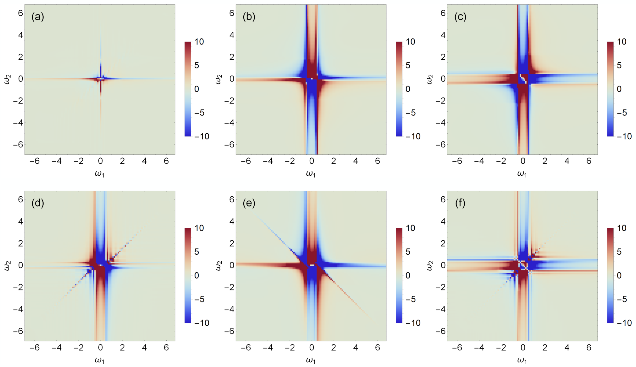
Figure 2: Two-dimensional Fourier spectrum of the four point correlation functions. Here ℱ\mathcal{F} is the Fourier transformation.
(a) Im​ℱ​[Im​Rz​z​z(1,2),z​(τ2,τ1,0)]\mathrm{Im}\,\mathcal{F}[\mathrm{Im}\,R^{(1,2),z}_{zzz}(\tau_{2},\tau_{1},0)] (b) Im​ℱ​[Im​Rz​z​z(3),z​(τ2,τ1,0)]\mathrm{Im}\,\mathcal{F}[\mathrm{Im}\,R^{(3),z}_{zzz}(\tau_{2},\tau_{1},0)] (c) Im​ℱ​[Im​Rz​z​z(4),z​(τ2,τ1,0)]\mathrm{Im}\,\mathcal{F}[\mathrm{Im}\,R^{(4),z}_{zzz}(\tau_{2},\tau_{1},0)]
(d) Im​ℱ​[Im​Rz​z​z(1),z​(τ2,0,τ1)]\mathrm{Im}\,\mathcal{F}[\mathrm{Im}\,R^{(1),z}_{zzz}(\tau_{2},0,\tau_{1})] (e) Im​ℱ​[Im​Rz​z​z(2,3),z​(τ2,0,τ1)]\mathrm{Im}\,\mathcal{F}[\mathrm{Im}\,R^{(2,3),z}_{zzz}(\tau_{2},0,\tau_{1})] (f) Im​ℱ​[Im​Rz​z​z(4),z​(τ2,0,τ1)]\mathrm{Im}\,\mathcal{F}[\mathrm{Im}\,R^{(4),z}_{zzz}(\tau_{2},0,\tau_{1})]

Results.—We compute the real-time four-point correlation functions on a periodic lattice with 125×125125\times 125 unit cells. Two-dimensional Fourier transform of the third-order susceptibilities (Fig. 1) and the four-point correlation functions (Fig. 2) are the main results of our work. Here we exclude the case |Q⟩=|G⟩|Q\rangle=|G\rangle in Eq. (18) where the four-point function becomes nothing but a product of the two two-point functions, e.g., ⟨σ^jz​σ^kz​σ^lz​σ^mz⟩=⟨σ^jz​σ^kz⟩​⟨σ^lz​σ^mz⟩\langle\hat{\sigma}^{z}_{j}\hat{\sigma}^{z}_{k}\hat{\sigma}^{z}_{l}\hat{\sigma}^{z}_{m}\rangle=\langle\hat{\sigma}^{z}_{j}\hat{\sigma}^{z}_{k}\rangle\langle\hat{\sigma}^{z}_{l}\hat{\sigma}^{z}_{m}\rangle, which can yield physically inconsistent results within the single matter fermion approximation.

There are three distinctive features in the third-order susceptibilities in Fourier space (Fig. 1). First, both χz​z​z(3),z​(ω2,ω1,0)\chi^{(3),z}_{zzz}(\omega_{2},\omega_{1},0) and χz​z​z(3),z​(ω2,0,ω1)\chi^{(3),z}_{zzz}(\omega_{2},0,\omega_{1}), which are the Fourier transforms of χz​z​z(3),z​(τ2,τ1,0)\chi^{(3),z}_{zzz}(\tau_{2},\tau_{1},0) and χz​z​z(3),z​(τ2,0,τ1)\chi^{(3),z}_{zzz}(\tau_{2},0,\tau_{1}) respectively, exhibit sharp vertical line signals at the two-flux gap, ω1=E2−E0\omega_{1}=E_{2}-E_{0}. Second, χz​z​z(3),z​(ω2,0,ω1)\chi^{(3),z}_{zzz}(\omega_{2},0,\omega_{1}) has three extended diagonal signals. Third, if we extrapolate these diagonal signals to ω1=0\omega_{1}=0, two of the three have an ω2\omega_{2} intercept equal to the four-flux gap ±(E4−E0)\pm(E_{4}-E_{0}), i.e., there are overall shifts in these two diagonal signals.

While the results in Figs. 1 and 2 are the direct Fourier transforms of the real-time correlation functions SM, we can identify which processes are responsible for these distinctive signals in the susceptibilities from the formal analytic expressions of the Fourier transformed correlation functions. For example, the Fourier transformation of Rz​z​z(3),z​(τ2,0,τ1)R^{(3),z}_{zzz}(\tau_{2},0,\tau_{1}) [Eq. (18)] can be written as

Rz​z​z(3),z​(ω2,0,ω1)=⋯\displaystyle R^{(3),z}_{zzz}(\omega_{2},0,\omega_{1})=\cdots
+∑j≠k∑P​Q​R⟨G|σ^jz|P⟩⟨P|σ^kz|Q⟩⟨Q|σ^kz|R⟩⟨R|σ^jz|G⟩\displaystyle+\sum_{j\neq k}\sum_{PQR}\langle G|\hat{\sigma}^{z}_{j}|P\rangle\langle P|\hat{\sigma}^{z}_{k}|Q\rangle\langle Q|\hat{\sigma}^{z}_{k}|R\rangle\langle R|\hat{\sigma}^{z}_{j}|G\rangle
×14​δ​(ω1+E2+εP−E0)​δ​(ω2+E4−E2−εR)\displaystyle\times\frac{1}{4}\delta(\omega_{1}+E_{2}+\varepsilon_{P}-E_{0})\delta(\omega_{2}+E_{4}-E_{2}-\varepsilon_{R})
+∑j≠k∑P​Q​R⟨G|σ^kz|P⟩⟨P|σ^jz|Q⟩⟨Q|σ^kz|R⟩⟨R|σ^jz|G⟩\displaystyle+\sum_{j\neq k}\sum_{PQR}\langle G|\hat{\sigma}^{z}_{k}|P\rangle\langle P|\hat{\sigma}^{z}_{j}|Q\rangle\langle Q|\hat{\sigma}^{z}_{k}|R\rangle\langle R|\hat{\sigma}^{z}_{j}|G\rangle
×14​δ​(ω1+E2+εP−E0)​δ​(ω2+E4−E2−εR),\displaystyle\times\frac{1}{4}\delta(\omega_{1}+E_{2}+\varepsilon_{P}-E_{0})\delta(\omega_{2}+E_{4}-E_{2}-\varepsilon_{R}), (19)

where EnE_{n} is the vacuum energy of the nn-flux state, εP⁡(R)\varepsilon_{P(R)} is the matter fermion energy, and the other contributions which cannot be written in terms of the delta functions are in (⋯\cdots). The delta function pieces would show no signal for −(E2−E0)<ω1<0-(E_{2}-E_{0})<\omega_{1}<0. Similarly, the complex conjugate pair Rz​z​z(3),z​(ω2,0,ω1)R^{(3),z}_{zzz}(\omega_{2},0,\omega_{1}) has no weight in 0<ω1<E2−E00<\omega_{1}<E_{2}-E_{0}. This is nothing but the well-known spin gap for spin excitations Knolle et al. 2014. If the first pulse B0B_{0} does not transfer enough energy to excite two adjacent fluxes, the Kitaev spin liquid remains in the ground state. Hence, for finite nonlinear responses, the first pulse B0B_{0} must transfer energy greater than the two-flux gap E2−E0E_{2}-E_{0}.

Another important feature, the shifted diagonal in Fig. 1(b), also comes from the Rz​z​z(3),z​(ω2,0,ω1)R^{(3),z}_{zzz}(\omega_{2},0,\omega_{1}) [Fig. 2(e)]. When εP=εR=ε\varepsilon_{P}=\varepsilon_{R}=\varepsilon, note that the matrix element ⟨G​|σ^jz​|P⟩​⟨P​|σ^kz​|Q⟩​⟨Q|​σ^kz|​R⟩​⟨R|​σ^jz|​G⟩=|⟨G​|σ^jz​|P⟩​⟨P|​σ^kz|​Q⟩|2≥0\langle G|\hat{\sigma}^{z}_{j}|P\rangle\langle P|\hat{\sigma}^{z}_{k}|Q\rangle\langle Q|\hat{\sigma}^{z}_{k}|R\rangle\langle R|\hat{\sigma}^{z}_{j}|G\rangle=|\langle G|\hat{\sigma}^{z}_{j}|P\rangle\langle P|\hat{\sigma}^{z}_{k}|Q\rangle|^{2}\geq 0. Hence, the summation over sites ∑j≠k\sum_{j\neq k}, equivalently the summation over all different four-flux configurations |Q⟩|Q\rangle excited by σ^jz\hat{\sigma}^{z}_{j} and σ^kz\hat{\sigma}^{z}_{k}, results in only constructive interference. Therefore we get the strongly enhanced signal when

ω1\displaystyle\omega_{1} =E0−E2−ε<0,\displaystyle=E_{0}-E_{2}-\varepsilon<0, (20)
ω2\displaystyle\omega_{2} =E2−E4+ε=−ω1−(E4−E0),\displaystyle=E_{2}-E_{4}+\varepsilon=-\omega_{1}-(E_{4}-E_{0}), (21)

which corresponds to the shifted diagonal with the slope of −1-1 and the ω2\omega_{2} intercept −(E4−E0)-(E_{4}-E_{0}). According to Eq. (20), the domain of the line is determined by the single matter fermion bandwidth and the two-flux gap, and this is confirmed by Figs. 1 (b) and 2 (e).

Following a similar logic, we can understand two-flux gaps and the other two coherent diagonal signals coming from Rz​z​z(1),z​(ω2,0,ω1)R^{(1),z}_{zzz}(\omega_{2},0,\omega_{1}) and Rz​z​z(4),z​(ω2,0,ω1)R^{(4),z}_{zzz}(\omega_{2},0,\omega_{1}), which have contributions with the constraints in the sum over intermediate states via δ⁡(ω1+E0−E2−εR)​δ​(ω2+E4−E2−εR)\delta(\omega_{1}+E_{0}-E_{2}-\varepsilon_{R})\delta(\omega_{2}+E_{4}-E_{2}-\varepsilon_{R}) and δ⁡(ω1+E0−E2−εR)​δ​(ω2+E0−E2−εP)\delta(\omega_{1}+E_{0}-E_{2}-\varepsilon_{R})\delta(\omega_{2}+E_{0}-E_{2}-\varepsilon_{P}), respectively. Rz​z​z(1),z​(ω2,0,ω1)R^{(1),z}_{zzz}(\omega_{2},0,\omega_{1}) yields the shifted diagonal ω2=ω1−(E4−E0)\omega_{2}=\omega_{1}-(E_{4}-E_{0}), and Rz​z​z(4),z​(ω2,0,ω1)R^{(4),z}_{zzz}(\omega_{2},0,\omega_{1}) gives ω2=ω1\omega_{2}=\omega_{1} from the constructive interference with εP=εR\varepsilon_{P}=\varepsilon_{R} for ω1≥E2−E0\omega_{1}\geq E_{2}-E_{0}.

Conclusion.—In this work, we have demonstrated how two-dimensional spectroscopy can be used to obtain useful information about fractionalized excitations in the Kitaev spin liquids, where the single spin-flip process excites a Majorana fermion and two fluxes in adjacent plaquettes. The spectroscopic signatures as a function of two frequencies, ω1\omega_{1} and ω2\omega_{2}, corresponding to the delay time of two successive magnetic pulses and the time of measurement, offer a clear identification of both the Majorana fermions and flux excitations. We demonstrated that the two-flux gap appears in ω1\omega_{1} and the shifted diagonal signal in the ω1\omega_{1}-ω2\omega_{2} plane has an ω2\omega_{2} intercept at the four-flux gap. Most importantly, the presence of the sharp diagonal signals is the direct consequence of the itinerant Majorana fermions. The domain of finite response in the two-frequency ω1\omega_{1}-ω2\omega_{2} plane is determined by a number of stringent conditions, which makes it possible to identify clear signatures of fractionalized excitations. It will be interesting to extend our work to other theoretical models of quantum spin liquids, that are not exactly solvable. Furthermore, the results reported here may be tested in a number of candidate materials for the Kitaev spin liquids Jackeli and Khaliullin 2009; Trebst; Witczak-Krempa et al. 2014; Winter et al. 2017; Rau et al. 2016; Takagi et al. 2019; Motome and Nasu 2020. We expect our results will shed significant light on the identification of fractionalized excitations and quantum spin liquids.

This work was supported by the NSERC of Canada and the Center for Quantum Materials at the University of Toronto. Y.B.K. is supported by the Killam Research Fellowship of the Canada Council for the Arts, and K.H.L is supported by the Institute for Basic Science (IBS) in Korea (IBS-R009-G1). We thank Center for Advanced Computation at Korea Institute for Advanced Study for providing computing resources for this work. We thank Y. Wan and N. P. Armitage for letting us know about their work. We also thank Masafumi Udagawa, Qiang-Hua Wang, Panagiotis P. Stavropoulos and Adarsh S. Patri for helpful discussion.

W.C. and K.H.L. contributed equally to this work.

References

Supplemental Materials for “Theory of Two-Dimensional Nonlinear Spectroscopy for the Kitaev Spin Liquid”

I Nonlinear susceptibilities from correlation functions

Two-dimensional spectroscopy measures nonlinear dynamical susceptibilities of correlated systems. In this section, we briefly review nonlinear response theory and derive the nonlinear susceptibilities from multi-spin correlation functions. More interested readers may refer to Ref. Mukamel 1995 and references therein. Here, we choose the unit ℏ=1\hbar=1.

Consider a Hamiltonian H^T​(t)=H^+V^​(t)\hat{H}_{T}(t)=\hat{H}+\hat{V}(t) with a weak light-matter interaction V^(t)=−𝐁(t)⋅𝐌^\hat{V}(t)=-\mathbf{B}(t)\cdot\hat{\mathbf{M}}. By treating the time-dependent potential V^​(t)\hat{V}(t) as a small perturbation, we solve the Liouville equation, i​∂tρ^=[H^T,ρ^]i\partial_{t}\hat{\rho}=[\hat{H}_{T},\hat{\rho}], to get the magnetization induced by the incoming magnetic fields. Because of the structural similarity between the Liouville equation and the Schrödinger equation (i​∂tψ=H^T​ψi\partial_{t}\psi=\hat{H}_{T}\psi), the Liouville equation can be considered as the “Schrödinger equation” i​∂tρ^=LT​ρ^i\partial_{t}\hat{\rho}=L_{T}\hat{\rho} in a vector space of density operators, so called the Liouville space, with the superoperator LT:ρ^↦[H^T,ρ^]L_{T}:\hat{\rho}\mapsto[\hat{H}_{T},\hat{\rho}]. Hence, with the analogy H^T↔LT\hat{H}_{T}\leftrightarrow L_{T}, we can adopt known time-dependent perturbation theory for wavefunctions in the Hilbert space to solve for density operators in the Liouville space.

In the interaction picture, the operator evolves as 𝒪^I​(t)=ei​H^​(t−t0)​𝒪^​e−i​H^​(t−t0)\hat{\mathcal{O}}_{I}(t)=e^{i\hat{H}(t-t_{0})}\hat{\mathcal{O}}e^{-i\hat{H}(t-t_{0})} while the density operator obeys

i​∂ρ^I∂t=[V^I​(t),ρ^I​(t)].\displaystyle i\frac{\partial\hat{\rho}_{I}}{\partial t}=[\hat{V}_{I}(t),\hat{\rho}_{I}(t)]. (S1)

So the Dyson series in the Liouville space is ρ^I​(t)=∑n=0∞ρ^I(n)​(t)\hat{\rho}_{I}(t)=\sum_{n=0}^{\infty}\hat{\rho}_{I}^{(n)}(t), where

ρ^I(0)​(t)=ρ^​(t0)=|G⟩​⟨G|,\displaystyle\hat{\rho}_{I}^{(0)}(t)=\hat{\rho}(t_{0})=|G\rangle\langle G|, (S2)
ρ^I(1)(t)=−i∫t0t[V^I(t1),ρ^(t0)]dt1,\displaystyle\hat{\rho}_{I}^{(1)}(t)=-i\int_{t_{0}}^{t}[\hat{V}_{I}(t_{1}),\hat{\rho}(t_{0})]dt_{1}, (S3)
ρ^I(n>1)(t)=(−i)n∫t0t∫t0tn⋯∫t0t2[V^I(tn),[V^I(tn−1),[⋯,[V^I(t1),ρ^(t0)]⋯]]]dt1⋯dtn\displaystyle\hat{\rho}_{I}^{(n>1)}(t)=\left(-i\right)^{n}\int_{t_{0}}^{t}\int_{t_{0}}^{t_{n}}\cdots\int_{t_{0}}^{t_{2}}[\hat{V}_{I}(t_{n}),[\hat{V}_{I}(t_{n-1}),[\cdots,[\hat{V}_{I}(t_{1}),\hat{\rho}(t_{0})]\cdots]]]dt_{1}\cdots dt_{n} (S4)

if we prepared the ground state of H^\hat{H}, ρ^​(t0)=|G⟩​⟨G|\hat{\rho}(t_{0})=|G\rangle\langle G|, at time t=t0t=t_{0}. Then the induced magnetization is Mα​(t)=∑n=0∞M(n),α​(t)M^{\alpha}(t)=\sum_{n=0}^{\infty}M^{(n),\alpha}(t), where the nnth order contribution to the induced magnetization is

M(n),α=Tr⁡(M^Iα​(t)​ρ^I(n)​(t))\displaystyle M^{(n),\alpha}=\mathrm{Tr}\left(\hat{M}^{\alpha}_{I}(t)\hat{\rho}_{I}^{(n)}(t)\right) (S5)
=in∫t0t∫t0tn⋯∫t0t2Tr(M^Iα(t)[M^Iαn(tn),[⋯,[M^Iα1(t1),ρ^(t0)]⋯]])Bαn(tn)⋯Bα1(t1)dt1⋯dtn\displaystyle=i^{n}\int_{t_{0}}^{t}\int_{t_{0}}^{t_{n}}\cdots\int_{t_{0}}^{t_{2}}\mathrm{Tr}\left(\hat{M}^{\alpha}_{I}(t)[\hat{M}^{\alpha_{n}}_{I}(t_{n}),[\cdots,[\hat{M}^{\alpha_{1}}_{I}(t_{1}),\hat{\rho}(t_{0})]\cdots]]\right)B^{\alpha_{n}}(t_{n})\cdots B^{\alpha_{1}}(t_{1})~dt_{1}\cdots dt_{n} (S6)
=in∫t0t∫t0tn⋯∫t0t2Tr([[⋯[M^Iα(t),M^Iαn(tn)],⋯],M^Iα1(t1)]ρ^(t0))Bαn(tn)⋯Bα1(t1)dt1⋯dtn.\displaystyle=i^{n}\int_{t_{0}}^{t}\int_{t_{0}}^{t_{n}}\cdots\int_{t_{0}}^{t_{2}}\mathrm{Tr}\left([[\cdots[\hat{M}^{\alpha}_{I}(t),\hat{M}^{\alpha_{n}}_{I}(t_{n})],\cdots],\hat{M}^{\alpha_{1}}_{I}(t_{1})]\hat{\rho}(t_{0})\right)B^{\alpha_{n}}(t_{n})\cdots B^{\alpha_{1}}(t_{1})~dt_{1}\cdots dt_{n}. (S7)

To simplify the expression, let us introduce new variables τm=tm+1−tm\tau_{m}=t_{m+1}-t_{m}, tn+1≡tt_{n+1}\equiv t and take the limit t0→−∞t_{0}\to-\infty. Then we can deduce the nonlinear magnetization from the multi-spin correlation functions:

M(n),α(t)=Nsite∫0∞⋯∫0∞χαn,…,α1(n),α(τn,…,τ1)Bαn(t−τn)⋯Bα1(t−τn−τn−1−…−τ1),\displaystyle M^{(n),\alpha}(t)=N_{\text{site}}\int_{0}^{\infty}\cdots\int_{0}^{\infty}\chi^{(n),\alpha}_{\alpha_{n},...,\alpha_{1}}(\tau_{n},...,\tau_{1})B^{\alpha_{n}}(t-\tau_{n})\cdots B^{\alpha_{1}}(t-\tau_{n}-\tau_{n-1}-...-\tau_{1}), (S8)

with the nnth order nonlinear susceptibility

χαn,…,α1(n),α​(τn,…,τ1)\displaystyle\chi^{(n),\alpha}_{\alpha_{n},...,\alpha_{1}}(\tau_{n},...,\tau_{1}) =inNsiteθ(τn)⋯θ(τ1)Tr([[⋯[M^Iα(τn+…+τ1),M^Iαn(τn−1+…+τ1)],⋯],M^Iα1(0)]ρ^(−∞))\displaystyle=\frac{i^{n}}{N_{\text{site}}}\theta(\tau_{n})\cdots\theta(\tau_{1})\mathrm{Tr}\left([[\cdots[\hat{M}^{\alpha}_{I}(\tau_{n}+...+\tau_{1}),\hat{M}^{\alpha_{n}}_{I}(\tau_{n-1}+...+\tau_{1})],\cdots],\hat{M}^{\alpha_{1}}_{I}(0)]\hat{\rho}(-\infty)\right)
=inNsiteθ(τn)⋯θ(τ1)⟨G|[[⋯[M^Iα(τn+…+τ1),M^Iαn(τn−1+…+τ1)],⋯],M^Iα1(0)]|G⟩,\displaystyle=\frac{i^{n}}{N_{\text{site}}}\theta(\tau_{n})\cdots\theta(\tau_{1})\langle G|[[\cdots[\hat{M}^{\alpha}_{I}(\tau_{n}+...+\tau_{1}),\hat{M}^{\alpha_{n}}_{I}(\tau_{n-1}+...+\tau_{1})],\cdots],\hat{M}^{\alpha_{1}}_{I}(0)]|G\rangle, (S9)

where θ⁡(x)\theta(x) is the Heaviside step function imposing the causality.

II Physical Hilbert space of the Kitaev model

The Kitaev model is solved exactly by the Majorana fermion representation of the spin operators, σ^jα=i​bjα​cj\hat{\sigma}_{j}^{\alpha}=ib_{j}^{\alpha}c_{j},

H^=−∑α​-bondσjασkα⇒H~=∑α​-bond(ibjαbkα)(icjck)≡∑α​-bondiu^j​kαcjck\displaystyle\hat{H}=-\sum_{\alpha\text{-bond}}\sigma_{j}^{\alpha}\sigma_{k}^{\alpha}\Rightarrow\widetilde{H}=\sum_{\alpha\text{-bond}}(ib_{j}^{\alpha}b_{k}^{\alpha})(ic_{j}c_{k})\equiv\sum_{\alpha\text{-bond}}i\hat{u}^{\alpha}_{jk}c_{j}c_{k} (S10)

where {bjα,bkβ}=2​δj​k​δα​β\{b_{j}^{\alpha},b_{k}^{\beta}\}=2\delta_{jk}\delta^{\alpha\beta}, {bjα,ck}=0\{b_{j}^{\alpha},c_{k}\}=0, and {cj,ck}=2​δj​k\{c_{j},c_{k}\}=2\delta_{jk}. Since the ℤ2\mathbb{Z}_{2} gauge fields u^j​kα\hat{u}^{\alpha}_{jk} commute with H~\widetilde{H} and themselves, the fermionic Hilbert space ℋ=ℋF⊗ℋM\mathcal{H}=\mathcal{H}_{F}\otimes\mathcal{H}_{M} is factorized into the gauge or flux sector ℋF\mathcal{H}_{F} and the matter fermion sector ℋM\mathcal{H}_{M}.

To represent the gauge configurations {u^j​kα}\{\hat{u}_{jk}^{\alpha}\}, we introduce a complex bond fermion at each bond

χ⟨j​k⟩α=12(bjα+ibkα),χ⟨j​k⟩α†=12(bjα−ibkα),\displaystyle\chi_{\langle jk\rangle}^{\alpha}=\frac{1}{2}\left(b_{j}^{\alpha}+ib_{k}^{\alpha}\right),~\chi_{\langle jk\rangle}^{\alpha\dagger}=\frac{1}{2}\left(b_{j}^{\alpha}-ib_{k}^{\alpha}\right), (S11)

where site jj, kk belongs to the sublattice s=As=A and s=Bs=B, respectively Baskaran et al. 2007. Then u^j​kα=2​χ⟨j​k⟩α†​χ⟨j​k⟩α−1\hat{u}_{jk}^{\alpha}=2\chi_{\langle jk\rangle_{\alpha}}^{\dagger}\chi_{\langle jk\rangle_{\alpha}}-1. Therefore, the Hilbert space for the ℤ2\mathbb{Z}_{2} gauge fields u^j​kα\hat{u}_{jk}^{\alpha} is equivalent to the 23​N2^{3N}-dimensional fermionic Hilbert space ℋF=span​{|F⟩}\mathcal{H}_{F}=\mathrm{span}\left\{|F\rangle\right\} for χ⟨j​k⟩α\chi^{\alpha}_{\langle jk\rangle}, where

|F⟩=∏⟨j​k⟩(χ⟨j​k⟩α)n⟨j​k⟩|F0⟩\displaystyle\left|F\right\rangle=\prod_{{\langle jk\rangle}}\left(\chi^{\alpha}_{\langle jk\rangle}\right)^{n_{\langle jk\rangle}}\left|F_{0}\right\rangle (S12)

with n⟨j​k⟩α=0,1n_{{\langle jk\rangle}_{\alpha}}=0,1 and the zero-flux sector |F0⟩|F_{0}\rangle such that χ⟨j​k⟩α†|F0⟩=0\chi^{\alpha\dagger}_{\langle jk\rangle}|F_{0}\rangle=0 for all bonds ⟨j​k⟩\langle jk\rangle.

After we fix the gauge for a given flux sector, H~\widetilde{H} becomes an exactly solvable free fermion Hamiltonian

H~u\displaystyle\widetilde{H}_{u} =i2​∑μ,νMμ​ν​cμ,A​cν,B=i4​[𝐜AT𝐜BT]​[0M−MT0]​[𝐜A𝐜B],\displaystyle=\frac{i}{2}\sum_{\mu,\nu}M_{\mu\nu}c_{\mu,A}c_{\nu,B}=\frac{i}{4}\begin{bmatrix}\mathbf{c}_{A}^{T}&\mathbf{c}_{B}^{T}\end{bmatrix}\begin{bmatrix}0&M\\ -M^{T}&0\end{bmatrix}\begin{bmatrix}\mathbf{c}_{A}\\ \mathbf{c}_{B}\end{bmatrix}, (S13)

where a real matrix Mμ​ν=2​uμ​ναM_{\mu\nu}=2u_{\mu\nu}^{\alpha} for the α\alpha-bond and zero otherwise, and μ,ν=1,…,N\mu,\nu=1,...,N label the unit cell, i.e., j=(μ,s)j=(\mu,s). H~u\widetilde{H}_{u} can be block-diagonalized by a special orthogonal transformation Q∈O⁡(2​N)Q\in O(2N) Kitaev 2006; Zschocke and Vojta 2015. To be specific,

H~u\displaystyle\widetilde{H}_{u} =i4​[𝐜AT𝐜BT]​[0M−MT0]​[𝐜A𝐜B]=i4​[𝐜AT𝐜BT]​[0U​S​VT−V​S​UT0]​[𝐜A𝐜B]\displaystyle=\frac{i}{4}\begin{bmatrix}\mathbf{c}_{A}^{T}&\mathbf{c}_{B}^{T}\end{bmatrix}\begin{bmatrix}0&M\\ -M^{T}&0\end{bmatrix}\begin{bmatrix}\mathbf{c}_{A}\\ \mathbf{c}_{B}\end{bmatrix}=\frac{i}{4}\begin{bmatrix}\mathbf{c}_{A}^{T}&\mathbf{c}_{B}^{T}\end{bmatrix}\begin{bmatrix}0&USV^{T}\\ -VSU^{T}&0\end{bmatrix}\begin{bmatrix}\mathbf{c}_{A}\\ \mathbf{c}_{B}\end{bmatrix} (S14)
=i4​[𝐜AT𝐜BT]​[U00V]​[0S−S0]​[U00V]T​[𝐜A𝐜B]≡i4​[𝐜AT𝐜BT]​Q​[0S−S0]​QT​[𝐜A𝐜B]\displaystyle=\frac{i}{4}\begin{bmatrix}\mathbf{c}_{A}^{T}&\mathbf{c}_{B}^{T}\end{bmatrix}\begin{bmatrix}U&0\\ 0&V\end{bmatrix}\begin{bmatrix}0&S\\ -S&0\end{bmatrix}\begin{bmatrix}U&0\\ 0&V\end{bmatrix}^{T}\begin{bmatrix}\mathbf{c}_{A}\\ \mathbf{c}_{B}\end{bmatrix}\equiv\frac{i}{4}\begin{bmatrix}\mathbf{c}_{A}^{T}&\mathbf{c}_{B}^{T}\end{bmatrix}Q\begin{bmatrix}0&S\\ -S&0\end{bmatrix}Q^{T}\begin{bmatrix}\mathbf{c}_{A}\\ \mathbf{c}_{B}\end{bmatrix} (S15)
=i4​[(𝐛′)T(𝐛′′)T]​[0S−S0]​[𝐛′𝐛′′]=i2​∑m=1Nεm​bm′​bm′′=∑m=1Nεm​(am†​am−12),\displaystyle=\frac{i}{4}\begin{bmatrix}(\mathbf{b^{\prime}})^{T}&(\mathbf{b^{\prime\prime}})^{T}\end{bmatrix}\begin{bmatrix}0&S\\ -S&0\end{bmatrix}\begin{bmatrix}\mathbf{b^{\prime}}\\ \mathbf{b^{\prime\prime}}\end{bmatrix}=\frac{i}{2}\sum_{m=1}^{N}\varepsilon_{m}b^{\prime}_{m}b^{\prime\prime}_{m}=\sum_{m=1}^{N}\varepsilon_{m}\left(a_{m}^{\dagger}a_{m}-\frac{1}{2}\right), (S16)

where 𝐜s=[c1,s,c2,s,…,cN,s]T\mathbf{c}_{s}=\left[c_{1,s},c_{2,s},...,c_{N,s}\right]^{T} for s=A,Bs=A,B. bm′b^{\prime}_{m}, bm′′b^{\prime\prime}_{m} are the normal modes, and am†=12​(bm′−i​bm′′)a_{m}^{\dagger}=\frac{1}{2}\left(b^{\prime}_{m}-ib^{\prime\prime}_{m}\right), am=12​(bm′+i​bm′′)a_{m}=\frac{1}{2}\left(b^{\prime}_{m}+ib^{\prime\prime}_{m}\right) are the creation and annihilation operators of the complex matter fermion. The special orthogonal transformation Q=[U00V]Q=\begin{bmatrix}U&0\\ 0&V\end{bmatrix} is derived from the singular value decomposition of M=U​S​VTM=USV^{T} Zschocke and Vojta 2015. The matter fermion excitation energies εm≥0\varepsilon_{m}\geq 0 are the singular values S=diag​(ε1,…,εN)S=\text{diag}(\varepsilon_{1},...,\varepsilon_{N}), and the 2N2^{N}-dimensional matter fermion Hilbert space ℋM\mathcal{H}_{M} is spanned by ∏m=1N(am†)nm​|M0⟩\prod_{m=1}^{N}\left(a_{m}^{\dagger}\right)^{n_{m}}|M_{0}\rangle, nm=0,1n_{m}=0,1 with the matter vacuum |M0⟩|M_{0}\rangle satisfying am​|M0⟩=0a_{m}|M_{0}\rangle=0 for all mm. The matter vacuum and the creation and annihilation operators are implicitly dependent on the background gauge field configuration {u⟨j​k⟩α}\left\{u^{\alpha}_{\langle jk\rangle}\right\} or equivalently {n⟨j​k⟩}\left\{n_{\langle jk\rangle}\right\}.

It is important to note that eigenstates of the gauge-fixed Hamiltonian H~u\widetilde{H}_{u} are not physical eigenstates of the original Hamiltonian H^\hat{H}. After we represent the spin operators with Majorana fermions, we enlarged the 22​N2^{2N}-dimensional Hilbert space ℋphys\mathcal{H}_{\text{phys}} for the spins σ^jα\hat{\sigma}_{j}^{\alpha} to the 42​N4^{2N}-dimensional Hilbert space ℋF⊗ℋM\mathcal{H}_{F}\otimes\mathcal{H}_{M} for the bond fermions χ⟨j​k⟩α\chi^{\alpha}_{\langle jk\rangle} in ℋF\mathcal{H}_{F} and the matter fermions ama_{m} in ℋM\mathcal{H}_{M}. So not every wavefunction in the enlarged Hilbert space can be physically relevant. The gauge theory H~\widetilde{H} is a faithful representation of H^\hat{H} only if we restrict the theory to the gauge invariant subspace, i.e., a physical wavefunction |Ψphys⟩|\Psi_{\text{phys}}\rangle needs to be gauge invariant such that D^j​|Ψphys⟩=+|Ψphys⟩\hat{D}_{j}|\Psi_{\text{phys}}\rangle=+|\Psi_{\text{phys}}\rangle under a ℤ2\mathbb{Z}_{2} gauge transformation D^j=bjx​bjy​bjz​cj\hat{D}_{j}=b_{j}^{x}b_{j}^{y}b_{j}^{z}c_{j} for every site jj Kitaev 2006. Since the gauge transformation D^j\hat{D}_{j} flips sign of the gauge fields u^j​kx,y,z→−u^j​kx,y,z\hat{u}_{jk}^{x,y,z}\to-\hat{u}_{jk}^{x,y,z} and the itinerant Majorana fermion cj→−cjc_{j}\to-c_{j} at the site jj, the eigenstates of the gauge-fixed Hamiltonian are not gauge-invariant. To get the physical wavefunction |Ψphys⟩|\Psi_{\text{phys}}\rangle, we must project the gauge-fixed eigenstate |ψu⟩|\psi_{u}\rangle to the physical Hilbert space using the projection operator P^=S^​P^0\hat{P}=\hat{S}\hat{P}_{0}:

|Ψphys⟩\displaystyle|\Psi_{\text{phys}}\rangle =P^​|ψu⟩=(122​N−1​∑g∏j∈gD^j)​(1+D^2)​|ψu⟩≡S^​P^0​|ψu⟩,\displaystyle=\hat{P}|\psi_{u}\rangle=\left(\frac{1}{\sqrt{2^{2N-1}}}\sum_{g}\prod_{j\in g}\hat{D}_{j}\right)\left(\frac{1+\hat{D}}{2}\right)|\psi_{u}\rangle\equiv\hat{S}\hat{P}_{0}|\psi_{u}\rangle, (S17)

where gg is a collection of all possible proper subset of the lattice and D^=∏jD^j\hat{D}=\prod_{j}\hat{D}_{j}. Here S^\hat{S} symmetrically sums over all 22​N−12^{2N-1} number of physically equivalent eigenstates |ψu′⟩|\psi_{u^{\prime}}\rangle of differently gauge-fixed Hamiltonians H~u′\widetilde{H}_{u^{\prime}}, and P^0\hat{P}_{0} projects out all unphysical states |Ψunphys⟩|\Psi_{\mathrm{unphys}}\rangle with D^j​|Ψunphys⟩=−|Ψunphys⟩\hat{D}_{j}|\Psi_{\mathrm{unphys}}\rangle=-|\Psi_{\mathrm{unphys}}\rangle for some jj. Among 42​N=22​N×22​N−1×24^{2N}=2^{2N}\times 2^{2N-1}\times 2 degrees of freedom in ℋ\mathcal{H}, 22​N−12^{2N-1} are gauge copies of the same physical state, and only a half of the degrees of freedom with Dj^=+1\hat{D_{j}}=+1 are physical.

It has been shown that we can express P^0=12​(1+D^)\hat{P}_{0}=\frac{1}{2}\left(1+\hat{D}\right) in terms of matter fermion parity, π^=(−1)∑mam†​am\hat{\pi}=(-1)^{\sum_{m}a^{\dagger}_{m}a_{m}},

D^=(−1)θ​(∏⟨j​k⟩uj​kα)​(∏μi​cμ,A​cμ,B)=(−1)θ​(det​Q​∏⟨j​k⟩uj​kα)​π^,\displaystyle\hat{D}=(-1)^{\theta}\left(\prod_{\langle jk\rangle}u^{\alpha}_{jk}\right)\left(\prod_{\mu}ic_{\mu,A}c_{\mu,B}\right)=(-1)^{\theta}\left(\mathrm{det}\,Q\prod_{\langle jk\rangle}u^{\alpha}_{jk}\right)\hat{\pi}, (S18)

where (−1)θ(-1)^{\theta} is determined by the boundary condition, and QQ is the special orthogonal transformation to diagonalize H~u\widetilde{H}_{u} Pedrocchi et al. 2011. Since the gauge transformation D^j\hat{D}_{j} flips the sign of u^j​kα\hat{u}_{jk}^{\alpha} and cjc_{j}, the parity of bb fermions (which is equal to the parity of the bond fermions χα\chi^{\alpha}, π^b=π^χ=∏⟨j​k⟩uj​kα\hat{\pi}_{b}=\hat{\pi}_{\chi}=\prod_{\langle jk\rangle}u^{\alpha}_{jk}) and the parity of cc fermions (π^c=∏μi​cμ,A​cμ,B\hat{\pi}_{c}=\prod_{\mu}ic_{\mu,A}c_{\mu,B}) are not gauge invariant. However, the parity of the complex matter fermion π^\hat{\pi} must be gauge invariant because the occupation number of ama_{m} determines the density of states which directly influences physical observables. Since D^\hat{D} is also gauge invariant, we can deduce which matter fermion parity π^\hat{\pi} is physical for a given flux sector by calculating det​Q​π^χ\mathrm{det}\,Q\,\hat{\pi}_{\chi}. With the standard gauge choice uj​kα=+1u^{\alpha}_{jk}=+1 for the zero flux sector, two-flux states and four-flux states can be created by flipping appropriate one and two zz-bonds, respectively. Hence, the zero-flux and four-flux states have the same χ\chi fermion parity π^χ\hat{\pi}_{\chi}, but the two-flux states have the opposite π^χ\hat{\pi}_{\chi}. We numerically calculated det​Q\mathrm{det}\,Q for various system sizes and found that the zero-, two-, and four-flux states have the same value of det​Q\mathrm{det}\,Q. Therefore the zero-flux and four-flux states should have the same matter fermion parity π^\hat{\pi}, but the two-flux states have the opposite matter fermion parity Zschocke and Vojta 2015.

III Matrix elements for spin operators

To calculate the four-point functions, the matrix elements of σ^jz\hat{\sigma}^{z}_{j} between the energy eigenstates are necessary. Let |Rμ⟩|R_{\mu}\rangle be the two-flux states with one matter fermion a¯r\overline{a}_{r} having energy εr\varepsilon_{r}, i.e., |Rμ⟩=P^​|F2⟩​(a¯r†​|M¯0⟩)=P^​χμz​a¯r†​|F0⟩​|M¯0⟩|R_{\mu}\rangle=\hat{P}|F_{2}\rangle(\overline{a}_{r}^{\dagger}|\overline{M}_{0}\rangle)=\hat{P}\chi_{\mu}^{z}\overline{a}_{r}^{\dagger}|F_{0}\rangle|\overline{M}_{0}\rangle, where χμz\chi_{\mu}^{z} is the bond fermion at the zz-bond of μ\muth unit cell, and |M¯0⟩|\overline{M}_{0}\rangle is the matter vacuum of H~u¯\widetilde{H}_{\overline{u}} with two-flux gauge configuration u¯\overline{u}. The matrix element of the spin operator Z^μ=σ^μ,Az+σ^μ,Bz\hat{Z}_{\mu}=\hat{\sigma}_{\mu,A}^{z}+\hat{\sigma}_{\mu,B}^{z} between the two-flux state |Rμ⟩|R_{\mu}\rangle and the ground state |G⟩=P^​|F0⟩​|M0⟩|G\rangle=\hat{P}|F_{0}\rangle|M_{0}\rangle is calculated in Ref. Zschocke and Vojta 2015:

⟨Rμ|σ^μ,Az+σ^μ,Bz|G⟩\displaystyle\langle R_{\mu}|\hat{\sigma}_{\mu,A}^{z}+\hat{\sigma}_{\mu,B}^{z}|G\rangle ≡⟨Rμ|Z^μ|G⟩=⟨M¯0|⟨F0|a¯rχμz†P^Z^μP^|F0⟩|M0⟩\displaystyle\equiv\langle R_{\mu}|\hat{Z}_{\mu}|G\rangle=\langle\overline{M}_{0}|\langle F_{0}|\overline{a}_{r}\chi_{\mu}^{z\dagger}\hat{P}\hat{Z}_{\mu}\hat{P}|F_{0}\rangle|M_{0}\rangle (S19)
=⟨M¯0|⟨F0|a¯rχμz†[i(χμz+χμz†)cμ,A+(χμz−χμz†)cμ,B](1+∑jDj+⋯)|F0⟩|M0⟩\displaystyle=\langle\overline{M}_{0}|\langle F_{0}|\overline{a}_{r}\chi_{\mu}^{z\dagger}\left[i(\chi_{\mu}^{z}+\chi_{\mu}^{z\dagger})c_{\mu,A}+(\chi_{\mu}^{z}-\chi_{\mu}^{z\dagger})c_{\mu,B}\right](1+\sum_{j}D_{j}+\cdots)|F_{0}\rangle|M_{0}\rangle (S20)
=⟨M¯0|a¯r​(i​cμ,A+cμ,B)|M0⟩.\displaystyle=\langle\overline{M}_{0}|\overline{a}_{r}(ic_{\mu,A}+c_{\mu,B})|M_{0}\rangle. (S21)

The matter fermion annihilation operator a¯r\overline{a}_{r} and its vacuum |M¯0⟩|\overline{M}_{0}\rangle in the two-flux sector can be written in terms of the creation and annihilation operator ar†a_{r}^{\dagger}, ara_{r} of the matter fermions and the matter vacuum |M0⟩|M_{0}\rangle in the zero-flux sector. With singular value decompositions of the two-flux Hamiltonian H~u¯=U¯2​S¯2​V¯2T\widetilde{H}_{\overline{u}}=\overline{U}_{2}\overline{S}_{2}\overline{V}_{2}^{T} and the zero-flux Hamiltonian H~u=U0​S0​V0T\widetilde{H}_{u}=U_{0}S_{0}V_{0}^{T},

|M¯0⟩\displaystyle|\overline{M}_{0}\rangle =|det​X¯|​e−12​am†​F¯m​n​an†​|M0⟩,\displaystyle=\sqrt{|\mathrm{det}\,\overline{X}|}e^{-\frac{1}{2}a_{m}^{\dagger}\overline{F}_{mn}a_{n}^{\dagger}}|M_{0}\rangle, (S22)
a¯r\displaystyle\overline{a}_{r} =X¯r​r′​ar′+Y¯r​r′​ar′†,\displaystyle=\overline{X}_{rr^{\prime}}a_{r^{\prime}}+\overline{Y}_{rr^{\prime}}a^{\dagger}_{r^{\prime}}, (S23)

where Einstein’s summation convention is assumed for the repeated Latin indices labelling the energy eigenstates, and X¯=12​(U¯2T​U0+V¯2T​V0)\overline{X}=\frac{1}{2}(\overline{U}_{2}^{T}U_{0}+\overline{V}_{2}^{T}V_{0}), Y¯=12​(U¯2T​U0−V¯2T​V0)\overline{Y}=\frac{1}{2}(\overline{U}_{2}^{T}U_{0}-\overline{V}_{2}^{T}V_{0}), F¯=(X¯)−1​Y¯\overline{F}=(\overline{X})^{-1}\overline{Y}. The cc Majorana fermion can be also expressed in terms of the zero-flux matter fermion,

cμ,A=(U0)μ,s​(as+as†),cμ,B=i​(V0)μ,s​(as†−as).\displaystyle c_{\mu,A}=(U_{0})_{\mu,s}(a_{s}+a_{s}^{\dagger}),~c_{\mu,B}=i(V_{0})_{\mu,s}(a_{s}^{\dagger}-a_{s}). (S24)

Therefore

⟨Rμ|Z^μ|G⟩\displaystyle\langle R_{\mu}|\hat{Z}_{\mu}|G\rangle =|det​X¯|​⟨M0|​(X¯r​r′​ar′+Y¯r​r′​ar′†)​(i​(U0+V0)μ,s​as†+i​(U0−V0)μ,s​as)​|M0⟩\displaystyle=\sqrt{|\mathrm{det}\,\overline{X}|}\langle M_{0}|(\overline{X}_{rr^{\prime}}a_{r^{\prime}}+\overline{Y}_{rr^{\prime}}a^{\dagger}_{r^{\prime}})(i(U_{0}+V_{0})_{\mu,s}a_{s}^{\dagger}+i(U_{0}-V_{0})_{\mu,s}a_{s})|M_{0}\rangle (S25)
=i​|det​X¯|​[(U0+V0)​(X¯)−1]μ,r\displaystyle=i\sqrt{|\mathrm{det}\,\overline{X}|}\left[(U_{0}+V_{0})(\overline{X})^{-1}\right]_{\mu,r} (S26)

Similarly, we can define the four-flux matter vacuum state |Qμ​ν⟩=P^​χμz​χνz​|F0⟩​|M0′⟩|Q_{\mu\nu}\rangle=\hat{P}\chi_{\mu}^{z}\chi_{\nu}^{z}|F_{0}\rangle|M_{0}^{\prime}\rangle. By following the similar calculations in Ref. Zschocke and Vojta 2015; Blaizot and Ripka 1986,

⟨Rν|σ^μ,Az+σ^μ,Bz|Qμ​ν⟩\displaystyle\langle R_{\nu}|\hat{\sigma}_{\mu,A}^{z}+\hat{\sigma}_{\mu,B}^{z}|Q_{\mu\nu}\rangle ≡⟨Rν|Z^μ|Qμ​ν⟩=⟨M¯0|⟨F0|a¯rχνz†P^Z^μP^χμzχνz|F0⟩|M0′⟩\displaystyle\equiv\langle R_{\nu}|\hat{Z}_{\mu}|Q_{\mu\nu}\rangle=\langle\overline{M}_{0}|\langle F_{0}|\overline{a}_{r}\chi_{\nu}^{z\dagger}\hat{P}\hat{Z}_{\mu}\hat{P}\chi_{\mu}^{z}\chi_{\nu}^{z}|F_{0}\rangle|M_{0}^{\prime}\rangle (S27)
=⟨M¯0|⟨F0|a¯rχνz†[i(χμz+χμz†)cμ,A+(χμz−χμz†)cμ,B](1+∑jDj+⋯)χμzχνz|F0⟩|M0′⟩\displaystyle=\langle\overline{M}_{0}|\langle F_{0}|\overline{a}_{r}\chi_{\nu}^{z\dagger}\left[i(\chi_{\mu}^{z}+\chi_{\mu}^{z\dagger})c_{\mu,A}+(\chi_{\mu}^{z}-\chi_{\mu}^{z\dagger})c_{\mu,B}\right](1+\sum_{j}D_{j}+\cdots)\chi_{\mu}^{z}\chi_{\nu}^{z}|F_{0}\rangle|M_{0}^{\prime}\rangle (S28)
=⟨M¯0|a¯r​(i​cμ,A−cμ,B)|M0′⟩=⋯=i​|det​X′|​[(U4′−V4′)​(X′)−1]μ,r,\displaystyle=\langle\overline{M}_{0}|\overline{a}_{r}(ic_{\mu,A}-c_{\mu,B})|M_{0}^{\prime}\rangle=\cdots=i\sqrt{|\mathrm{det}\,X^{\prime}|}\left[(U^{\prime}_{4}-V^{\prime}_{4})(X^{\prime})^{-1}\right]_{\mu,r}, (S29)

where U4′U_{4}^{\prime} and V4′V_{4}^{\prime} are the left and right singular matrices of the four-flux Hamiltonian H~u′=U4′​S4′​V4′T\widetilde{H}_{u^{\prime}}=U_{4}^{\prime}S_{4}^{\prime}{V_{4}^{\prime}}^{T}, and X′=12​(U¯2T​U4′+V¯2T​V4′)X^{\prime}=\frac{1}{2}(\overline{U}_{2}^{T}U_{4}^{\prime}+\overline{V}_{2}^{T}V_{4}^{\prime}). Note that |Qμ​ν⟩=−|Qν​μ⟩|Q_{\mu\nu}\rangle=-|Q_{\nu\mu}\rangle implies

⟨Rμ|σ^ν,Az+σ^ν,Bz|Qμ​ν⟩\displaystyle\langle R_{\mu}|\hat{\sigma}_{\nu,A}^{z}+\hat{\sigma}_{\nu,B}^{z}|Q_{\mu\nu}\rangle ≡⟨Rμ|Z^ν|Qμ​ν⟩=−⟨Rμ|Z^ν|Qν​μ⟩=−i​|det​X′|​[(U4′−V4′)​(X′)−1]ν,r.\displaystyle\equiv\langle R_{\mu}|\hat{Z}_{\nu}|Q_{\mu\nu}\rangle=-\langle R_{\mu}|\hat{Z}_{\nu}|Q_{\nu\mu}\rangle=-i\sqrt{|\mathrm{det}\,X^{\prime}|}\left[(U_{4}^{\prime}-V_{4}^{\prime})(X^{\prime})^{-1}\right]_{\nu,r}. (S30)

IV Real-time four-point correlation functions

We calculated the third-order nonlinear susceptibilities from the four-point correlation functions, which are mostly out of time order (Fig. S1).

Refer to caption
Figure S1: Real-time third-order susceptibilities (a) χz​z​z(3),z​(τ2,τ1,0)\chi^{(3),z}_{zzz}(\tau_{2},\tau_{1},0) (b) χz​z​z(3),z​(τ2,0,τ1)\chi^{(3),z}_{zzz}(\tau_{2},0,\tau_{1})
Refer to caption
Figure S2: Real-time dynamical correlation functions for the isotropic Kitaev model on a 125×125125\times 125 honeycomb lattice.
(a) Rz​z​z(1,2),z​(τ2,τ1,0)R^{(1,2),z}_{zzz}(\tau_{2},\tau_{1},0) (b) Rz​z​z(3),z​(τ2,τ1,0)R^{(3),z}_{zzz}(\tau_{2},\tau_{1},0) (c) Rz​z​z(4),z​(τ2,τ1,0)R^{(4),z}_{zzz}(\tau_{2},\tau_{1},0) (d) Rz​z​z(1),z​(τ2,0,τ1)R^{(1),z}_{zzz}(\tau_{2},0,\tau_{1}) (e) Rz​z​z(2,3),z​(τ2,0,τ1)R^{(2,3),z}_{zzz}(\tau_{2},0,\tau_{1}) (f) Rz​z​z(4),z​(τ2,0,τ1)R^{(4),z}_{zzz}(\tau_{2},0,\tau_{1})

Using the resolution of identity ∑P|P⟩​⟨P|=1\sum_{P}|P\rangle\langle P|=1 with the energy eigenstate |P⟩|P\rangle, we decompose each four-point function into a sum of products of four matrix elements of the spin operator. For example,

Rz​z​z(1),z​(τ2,τ1,0)\displaystyle R^{(1),z}_{zzz}(\tau_{2},\tau_{1},0) =⟨G|M^z​(0)​M^z​(τ1)​M^z​(τ2+τ1)​M^z​(0)|G⟩\displaystyle=\langle G|\hat{M}^{z}(0)\hat{M}^{z}(\tau_{1})\hat{M}^{z}(\tau_{2}+\tau_{1})\hat{M}^{z}(0)|G\rangle
=∑P​Q​R⟨G​|M^z​|P⟩​⟨P|ei​H^​τ1​M^z​e−i​H^​τ1|Q⟩​⟨Q|ei​H^​(τ2+τ1)​M^z​e−i​H^​(τ2+τ1)|R⟩​⟨R|​M^z|​G⟩\displaystyle=\sum_{PQR}\langle G|\hat{M}^{z}|P\rangle\langle P|e^{i\hat{H}\tau_{1}}\hat{M}^{z}e^{-i\hat{H}\tau_{1}}|Q\rangle\langle Q|e^{i\hat{H}(\tau_{2}+\tau_{1})}\hat{M}^{z}e^{-i\hat{H}(\tau_{2}+\tau_{1})}|R\rangle\langle R|\hat{M}^{z}|G\rangle (S31)
=∑P​Q​Rei⁡(EP−EQ)​τ1+i⁡(EQ−ER)​(τ2+τ1)​⟨G​|M^z​|P⟩​⟨P|M^z|Q⟩​⟨Q|M^z|R⟩​⟨R|​M^z|​G⟩\displaystyle=\sum_{PQR}e^{i(E_{P}-E_{Q})\tau_{1}+i(E_{Q}-E_{R})(\tau_{2}+\tau_{1})}\langle G|\hat{M}^{z}|P\rangle\langle P|\hat{M}^{z}|Q\rangle\langle Q|\hat{M}^{z}|R\rangle\langle R|\hat{M}^{z}|G\rangle (S32)
=∑μ​ν​λ​ρ∑Qei​EQ​τ2​∑Pei​EP​τ1​⟨G​|Z^μ​|P⟩​⟨P|Z^ν|Q⟩​∑Re−i​ER​(τ2+τ1)​⟨Q|Z^λ|R⟩​⟨R|​Z^ρ|​G⟩\displaystyle=\sum_{\mu\nu\lambda\rho}\sum_{Q}e^{iE_{Q}\tau_{2}}\sum_{P}e^{iE_{P}\tau_{1}}\langle G|\hat{Z}_{\mu}|P\rangle\langle P|\hat{Z}_{\nu}|Q\rangle\sum_{R}e^{-iE_{R}(\tau_{2}+\tau_{1})}\langle Q|\hat{Z}_{\lambda}|R\rangle\langle R|\hat{Z}_{\rho}|G\rangle (S33)

Since each operator Z^μ=σ^μ,Az+σ^μ,Bz\hat{Z}_{\mu}=\hat{\sigma}^{z}_{\mu,A}+\hat{\sigma}^{z}_{\mu,B} at a zz-bond of the μ\muth unit cell excites two fluxes adjacent to the zz-bond, we can infer the flux sectors of |P⟩|P\rangle, |Q⟩|Q\rangle, and |R⟩|R\rangle so that

Rz​z​z(1),z​(τ2,τ1,0)\displaystyle R^{(1),z}_{zzz}(\tau_{2},\tau_{1},0) =N​∑μei⁡(E0−E2)​τ2​∑Qei​εQ​τ2​∑Pei​εP​τ1​⟨G​|Z^μ​|P⟩​⟨P|Z^μ|Q⟩​∑Re−i​εR​(τ2+τ1)​⟨Q|Z^0|R⟩​⟨R|​Z^0|​G⟩\displaystyle=N\sum_{\mu}e^{i(E_{0}-E_{2})\tau_{2}}\sum_{Q}e^{i\varepsilon_{Q}\tau_{2}}\sum_{P}e^{i\varepsilon_{P}\tau_{1}}\langle G|\hat{Z}_{\mu}|P\rangle\langle P|\hat{Z}_{\mu}|Q\rangle\sum_{R}e^{-i\varepsilon_{R}(\tau_{2}+\tau_{1})}\langle Q|\hat{Z}_{0}|R\rangle\langle R|\hat{Z}_{0}|G\rangle (S34)
+N∑μ≠0ei⁡(E4​(μ)−E2)​τ2∑Qei​εQ​τ2∑Pei​εP​τ1⟨G|Z^0|P⟩⟨P|Z^μ|Q⟩∑Re−i​εR​(τ2+τ1)⟨Q|Z^μ|R⟩⟨R|Z^0|G⟩\displaystyle+N\sum_{\mu\neq 0}e^{i(E_{4}(\mu)-E_{2})\tau_{2}}\sum_{Q}e^{i\varepsilon_{Q}\tau_{2}}\sum_{P}e^{i\varepsilon_{P}\tau_{1}}\langle G|\hat{Z}_{0}|P\rangle\langle P|\hat{Z}_{\mu}|Q\rangle\sum_{R}e^{-i\varepsilon_{R}(\tau_{2}+\tau_{1})}\langle Q|\hat{Z}_{\mu}|R\rangle\langle R|\hat{Z}_{0}|G\rangle (S35)
+N∑μ≠0ei⁡(E4​(μ)−E2)​τ2∑Qei​εQ​τ2∑P~ei​εP~​τ1⟨G|Z^μ|P~⟩⟨P~|Z^0|Q⟩∑Re−i​εR​(τ2+τ1)⟨Q|Z^μ|R⟩⟨R|Z^0|G⟩,\displaystyle+N\sum_{\mu\neq 0}e^{i(E_{4}(\mu)-E_{2})\tau_{2}}\sum_{Q}e^{i\varepsilon_{Q}\tau_{2}}\sum_{\widetilde{P}}e^{i\varepsilon_{\widetilde{P}}\tau_{1}}\langle G|\hat{Z}_{\mu}|\widetilde{P}\rangle\langle\widetilde{P}|\hat{Z}_{0}|Q\rangle\sum_{R}e^{-i\varepsilon_{R}(\tau_{2}+\tau_{1})}\langle Q|\hat{Z}_{\mu}|R\rangle\langle R|\hat{Z}_{0}|G\rangle, (S36)

where E0E_{0} is the energy of the ground state |G⟩|G\rangle, and εP\varepsilon_{P}, εQ\varepsilon_{Q}, εR\varepsilon_{R} are the total matter fermion excitation energies of |P⟩|P\rangle, |Q⟩|Q\rangle, and |R⟩|R\rangle, respectively. E0E_{0}, E2E_{2}, E4​(μ)E_{4}(\mu) are the energies of the matter fermion vacuum states with the zero-flux, two-flux, and four-flux background. Note that E4​(μ)E_{4}(\mu) depends on the relative distance between two pairs of fluxes; two fluxes share the zz-bond at the 0th unit cell and the other two flux share the zz-bond at the μ\muth unit cell. Using translational symmetry of the zero flux states, we simplified the summation ∑ρ→N∑ρδρ,0\sum_{\rho}\to N\sum_{\rho}\delta_{\rho,0}. Similarly, we can decompose and reorganize the other correlation functions R(l=2,3,4)​(τ2,τ1,0)R^{(l=2,3,4)}(\tau_{2},\tau_{1},0) and R(l=1,2,3,4)​(τ2,0,τ1)R^{(l=1,2,3,4)}(\tau_{2},0,\tau_{1}).

After we approximate the correlation function by truncating the summation ∑P​Q​R\sum_{PQR} up to one-matter-fermion states, we calculated the four-point functions from τ1,2=0\tau_{1,2}=0 to τ1,2=60\tau_{1,2}=60 with d​τ=0.25d\tau=0.25 (Fig. S2). To calculate the matrix elements, Eqs. (S26), (S29), and (S30), singular value decompositions (SVDs) of N×NN\times N matrices, of which calculation complexity is 𝒪⁡(N3)=𝒪⁡(L6)\mathcal{O}(N^{3})=\mathcal{O}(L^{6}), are necessary for N=L×LN=L\times L unit-cell cluster of the honeycomb lattice. For Eqs. (S35) and (S36), N−1N-1 number of all different four-flux configurations |Q⟩|Q\rangle must be summed over because of ∑μ≠0\sum_{\mu\neq 0}. For a given μ\mu, two different SVDs are necessary for the two-flux state |P~⟩|\widetilde{P}\rangle and the four-flux state |Q⟩|Q\rangle. Therefore the computational cost quickly grows as 𝒪⁡(L8)\mathcal{O}(L^{8}) even after the summation is truncated. Ripple-like anomalous long time behavior is finite size effect Wan and Armitage 2019, so we truncate the real-time correlation functions and use the fast Fourier transformations (FFT) to obtain the two-dimensional Fourier spectra for the third-order susceptibilities. The diagonal signals in the first and third quadrants originating from R(1)​(τ2,0,τ1)R^{(1)}(\tau_{2},0,\tau_{1}) and R(4)​(τ2,0,τ1)R^{(4)}(\tau_{2},0,\tau_{1}) [Fig. 2 (d) and (f) of the Letter] are sensitive to how we truncate the two-dimensional real-time susceptibilities before the Fourier transformations. However, the sharp diagonal signals in the second and fourth quadrants due to R(3)​(τ2,0,τ1)R^{(3)}(\tau_{2},0,\tau_{1}) [Fig. 2 (e) of the Letter] are robust and hardly dependent to the way we crop the real-time data.