f-electron charge densities
probed using
core level non-resonant inelastic x-ray scattering
D I S S E R T A T I O N
– überarbeitete Fassung –
von
Martin Sundermann
| Vorgelegt der Fakultät Mathematik und Naturwissenschaften |
| der Technischen Universität Dresden |
| Eingereicht am: | 15.11.2018 |
| Tag der Verteidigung: | 05.06.2019 |
| Gutachter: |
| Prof. Dr. L. H. Tjeng |
| Max-Planck-Institut für Chemische Physik fester Stoffe, Dresden |
| Prof. Dr. J. Geck |
| Technische Universität Dresden |
| Prof. Dr. M. W. Haverkort |
| Universität Heidelberg |
Abstract
Strongly correlated materials are characterized by the presence of electron-electron interactions in their electronic structure. They often have remarkable properties and transitions between competing phases of very different electronic and magnetic order. This thesis focuses on strongly correlated f-electron compounds containing Ce, Sm, and U. These materials exhibit a so-called heavy-fermion or Kondo-lattice behavior. They can become insulating due to hybridization effects (Kondo-insulator) or develop multipolar (hidden) order. Kondo insulators have recently been discussed in the context of strongly correlated topological insulators. This new aspect caused an enormous activity in the field of Kondo insulators, theoretically as well as experimentally.
Multipolar order as well as the formation of a Kondo insulating state strongly depend on the symmetry of the states involved. Also the character of the surface states in a topological insulator is determined by the properties of the bulk states. Therefore the scope of this thesis has been to unveil the underlying symmetries of the bulk states. Here the compounds CeB6, UO2, and URu2Si2, which exhibit multipolar order, as well as the Kondo insulators (semimetals) SmB6 and CeRu4Sn6 have been studied.
Non-resonant inelastic x-ray scattering (\HyColor@XZeroOneThreeFour\pc@goptd@color\pc@hyenc@colorpdfcommentcolor\HyColor@XZeroOneThreeFour\pc@goptd@fontcolor\pc@hyenc@fontcolorpdfcommentcolor\HyColor@XZeroOneThreeFour\pc@goptd@icolor\pc@hyenc@icolorpdfcommentcolor\pdfmark[NIXS]pdfmark=/ANN,Subtype=/Widget,Raw=/TU (non-resonant inelastic x-ray scattering\textCR(\pc@goptd@deadline)) /T (tooltip zref@0) /C [ ] /FT/Btn /F 768 /Ff 65536 /H/N /BS << /W 0 >> ) has been established as a bulk sensitive technique for determining ground-state wave functions. \HyColor@XZeroOneThreeFour\pc@goptd@color\pc@hyenc@colorpdfcommentcolor\HyColor@XZeroOneThreeFour\pc@goptd@fontcolor\pc@hyenc@fontcolorpdfcommentcolor\HyColor@XZeroOneThreeFour\pc@goptd@icolor\pc@hyenc@icolorpdfcommentcolor\pdfmark[NIXS]pdfmark=/ANN,Subtype=/Widget,Raw=/TU (non-resonant inelastic x-ray scattering\textCR(\pc@goptd@deadline)) /T (tooltip zref@1) /C [ ] /FT/Btn /F 768 /Ff 65536 /H/N /BS << /W 0 >> at large momentum transfer measures a higher than dipole scattering signal, so that anisotropies of cubic point symmetries are accessible, and it is the only technique that shows multiplet structures in metallic uranium compounds.
CeB6 (Ch. 5) and UO2 (Ch. 8) were measured because they can serve as benchmark compounds; their ground states were known from other studies, so that the validity of the \HyColor@XZeroOneThreeFour\pc@goptd@color\pc@hyenc@colorpdfcommentcolor\HyColor@XZeroOneThreeFour\pc@goptd@fontcolor\pc@hyenc@fontcolorpdfcommentcolor\HyColor@XZeroOneThreeFour\pc@goptd@icolor\pc@hyenc@icolorpdfcommentcolor\pdfmark[NIXS]pdfmark=/ANN,Subtype=/Widget,Raw=/TU (non-resonant inelastic x-ray scattering\textCR(\pc@goptd@deadline)) /T (tooltip zref@2) /C [ ] /FT/Btn /F 768 /Ff 65536 /H/N /BS << /W 0 >> experiment and its analysis could be tested. For SmB6 (Ch. 6), CeRu4Sn6 (Ch. 7), and URu2Si2 (Ch. 9) the ground states were determined. For SmB6 \HyColor@XZeroOneThreeFour\pc@goptd@color\pc@hyenc@colorpdfcommentcolor\HyColor@XZeroOneThreeFour\pc@goptd@fontcolor\pc@hyenc@fontcolorpdfcommentcolor\HyColor@XZeroOneThreeFour\pc@goptd@icolor\pc@hyenc@icolorpdfcommentcolor\pdfmark[NIXS]pdfmark=/ANN,Subtype=/Widget,Raw=/TU (non-resonant inelastic x-ray scattering\textCR(\pc@goptd@deadline)) /T (tooltip zref@3) /C [ ] /FT/Btn /F 768 /Ff 65536 /H/N /BS << /W 0 >> was needed because SmB6 is cubic, for CeRu4Sn6 because \HyColor@XZeroOneThreeFour\pc@goptd@color\pc@hyenc@colorpdfcommentcolor\HyColor@XZeroOneThreeFour\pc@goptd@fontcolor\pc@hyenc@fontcolorpdfcommentcolor\HyColor@XZeroOneThreeFour\pc@goptd@icolor\pc@hyenc@icolorpdfcommentcolor\pdfmark[NIXS]pdfmark=/ANN,Subtype=/Widget,Raw=/TU (non-resonant inelastic x-ray scattering\textCR(\pc@goptd@deadline)) /T (tooltip zref@4) /C [ ] /FT/Btn /F 768 /Ff 65536 /H/N /BS << /W 0 >> is bulk sensitive, and for URu2Si2 because the multipolar \HyColor@XZeroOneThreeFour\pc@goptd@color\pc@hyenc@colorpdfcommentcolor\HyColor@XZeroOneThreeFour\pc@goptd@fontcolor\pc@hyenc@fontcolorpdfcommentcolor\HyColor@XZeroOneThreeFour\pc@goptd@icolor\pc@hyenc@icolorpdfcommentcolor\pdfmark[NIXS]pdfmark=/ANN,Subtype=/Widget,Raw=/TU (non-resonant inelastic x-ray scattering\textCR(\pc@goptd@deadline)) /T (tooltip zref@5) /C [ ] /FT/Btn /F 768 /Ff 65536 /H/N /BS << /W 0 >> signal is more excitonic.
Finally, the linear independent directions of the multipole expansion of the transition operator in \HyColor@XZeroOneThreeFour\pc@goptd@color\pc@hyenc@colorpdfcommentcolor\HyColor@XZeroOneThreeFour\pc@goptd@fontcolor\pc@hyenc@fontcolorpdfcommentcolor\HyColor@XZeroOneThreeFour\pc@goptd@icolor\pc@hyenc@icolorpdfcommentcolor\pdfmark[NIXS]pdfmark=/ANN,Subtype=/Widget,Raw=/TU (non-resonant inelastic x-ray scattering\textCR(\pc@goptd@deadline)) /T (tooltip zref@6) /C [ ] /FT/Btn /F 768 /Ff 65536 /H/N /BS << /W 0 >> have been investigated (Ch. 3.2.2) and a tensor notation has been developed (Ch. 3.4). This is useful for a better understanding of the directional dependence of the momentum transfer of the single crystal \HyColor@XZeroOneThreeFour\pc@goptd@color\pc@hyenc@colorpdfcommentcolor\HyColor@XZeroOneThreeFour\pc@goptd@fontcolor\pc@hyenc@fontcolorpdfcommentcolor\HyColor@XZeroOneThreeFour\pc@goptd@icolor\pc@hyenc@icolorpdfcommentcolor\pdfmark[NIXS]pdfmark=/ANN,Subtype=/Widget,Raw=/TU (non-resonant inelastic x-ray scattering\textCR(\pc@goptd@deadline)) /T (tooltip zref@7) /C [ ] /FT/Btn /F 768 /Ff 65536 /H/N /BS << /W 0 >> spectra.
Kurzzusammenfassung
Stark korrelierte Systeme werden stark von der Elektron-Elektron-Wechselwirkung geprägt. Dies führt häufig zu bemerkenswerten Eigenschaften und Übergängen zwischen konkurrierenden Phasen sehr unterschiedlicher elektronischer oder magnetischer Ordnung. Diese Dissertation behandelt stark korrelierte f-Elektronen-Systeme die Ce, Sm und U beinhalten. Diese weisen sogenanntes schwerfermionisches oder Kondo-Gitter-Verhalten auf. Sie können durch Hybridisierung isolierend werden (Kondo-Isolator) oder eine multipolare (verborgene) Ordnung ausbilden. Seit Kurzem werden Kondo-Isolatoren als mögliche stark korrelierte topologische Isolatoren diskutiert. Dieser neue Aspekt rief eine Vielzahl an Tätigkeiten im Bereich der Kondo-Isolatoren hervor, sowohl theoretisch als auch experimentell.
Sowohl multipolare Ordnung als auch die Formation des Kondo-isolierenden Zustandes hängen stark von der Symmetrie der f-Elektronen ab. Auch die Eigenschaften der Oberflächenzustände topologischer Isolatoren werden von den Zuständen im Inneren bestimmt. Daher befasst sich diese Dissertation mit der Identifizierung der Symmetrie der inneren f-Elekronen-Zustände. Es wurden CeB6, UO2 und URu2Si2, welche multipolare Ordnung aufweisen, sowie die Kondo-Isolatoren/Semi-metalle SmB6 und CeRu4Sn6 untersucht.
Nicht-resonante inelastische Röntgenstreuung (\HyColor@XZeroOneThreeFour\pc@goptd@color\pc@hyenc@colorpdfcommentcolor\HyColor@XZeroOneThreeFour\pc@goptd@fontcolor\pc@hyenc@fontcolorpdfcommentcolor\HyColor@XZeroOneThreeFour\pc@goptd@icolor\pc@hyenc@icolorpdfcommentcolor\pdfmark[NIXS]pdfmark=/ANN,Subtype=/Widget,Raw=/TU (non-resonant inelastic x-ray scattering\textCR(\pc@goptd@deadline)) /T (tooltip zref@8) /C [ ] /FT/Btn /F 768 /Ff 65536 /H/N /BS << /W 0 >> ) wurde als bulksensitive Methode zur Bestimmung der Grundzustandswellenfunktion etabliert. Für große Impulsüberträge weist NIXS Signale jenseits der Dipol-Auswahlregeln auf, sodass Anisotropien auch in kubischer Punktsymmetrie feststellbar sind, und zeigt als einzige Methode klare exzitonische Multiplettstrukturen für metallische Uranverbindungen.
CeB6 (Kap. 5) und UO2 (Kap. 8), deren Grundzustand bereits aus anderen Studien bekannt sind, wurden als Referenzmaterialien untersucht um die Gültigkeit der Methode und der Auswertung zu überprüfen. Für SmB6 (Kap. 6), CeRu4Sn6 (Kap. 7) und URu2Si2 (Kap. 9) wurden die Grundzustände bestimmt. Im Fall von SmB6 wurde \HyColor@XZeroOneThreeFour\pc@goptd@color\pc@hyenc@colorpdfcommentcolor\HyColor@XZeroOneThreeFour\pc@goptd@fontcolor\pc@hyenc@fontcolorpdfcommentcolor\HyColor@XZeroOneThreeFour\pc@goptd@icolor\pc@hyenc@icolorpdfcommentcolor\pdfmark[NIXS]pdfmark=/ANN,Subtype=/Widget,Raw=/TU (non-resonant inelastic x-ray scattering\textCR(\pc@goptd@deadline)) /T (tooltip zref@9) /C [ ] /FT/Btn /F 768 /Ff 65536 /H/N /BS << /W 0 >> benötigt da SmB6 kubisch ist, für CeRu4Sn6 da \HyColor@XZeroOneThreeFour\pc@goptd@color\pc@hyenc@colorpdfcommentcolor\HyColor@XZeroOneThreeFour\pc@goptd@fontcolor\pc@hyenc@fontcolorpdfcommentcolor\HyColor@XZeroOneThreeFour\pc@goptd@icolor\pc@hyenc@icolorpdfcommentcolor\pdfmark[NIXS]pdfmark=/ANN,Subtype=/Widget,Raw=/TU (non-resonant inelastic x-ray scattering\textCR(\pc@goptd@deadline)) /T (tooltip zref@10) /C [ ] /FT/Btn /F 768 /Ff 65536 /H/N /BS << /W 0 >> bulksensitiv ist und für URu2Si2 wegen des exzitonischen \HyColor@XZeroOneThreeFour\pc@goptd@color\pc@hyenc@colorpdfcommentcolor\HyColor@XZeroOneThreeFour\pc@goptd@fontcolor\pc@hyenc@fontcolorpdfcommentcolor\HyColor@XZeroOneThreeFour\pc@goptd@icolor\pc@hyenc@icolorpdfcommentcolor\pdfmark[NIXS]pdfmark=/ANN,Subtype=/Widget,Raw=/TU (non-resonant inelastic x-ray scattering\textCR(\pc@goptd@deadline)) /T (tooltip zref@11) /C [ ] /FT/Btn /F 768 /Ff 65536 /H/N /BS << /W 0 >> Signals.
Weiter wurden die linear unabhängigen Richtungen der multipolaren Übergänge des Übergangsmatrixelements von \HyColor@XZeroOneThreeFour\pc@goptd@color\pc@hyenc@colorpdfcommentcolor\HyColor@XZeroOneThreeFour\pc@goptd@fontcolor\pc@hyenc@fontcolorpdfcommentcolor\HyColor@XZeroOneThreeFour\pc@goptd@icolor\pc@hyenc@icolorpdfcommentcolor\pdfmark[NIXS]pdfmark=/ANN,Subtype=/Widget,Raw=/TU (non-resonant inelastic x-ray scattering\textCR(\pc@goptd@deadline)) /T (tooltip zref@12) /C [ ] /FT/Btn /F 768 /Ff 65536 /H/N /BS << /W 0 >> untersucht (Kap. 3.2.2) und eine Tensorschreibweise entwickelt (Kap. 3.4). Dies erlaubt ein besseres Verständnis der Richtungsabhängigkeit des Impulsübertrages der \HyColor@XZeroOneThreeFour\pc@goptd@color\pc@hyenc@colorpdfcommentcolor\HyColor@XZeroOneThreeFour\pc@goptd@fontcolor\pc@hyenc@fontcolorpdfcommentcolor\HyColor@XZeroOneThreeFour\pc@goptd@icolor\pc@hyenc@icolorpdfcommentcolor\pdfmark[NIXS]pdfmark=/ANN,Subtype=/Widget,Raw=/TU (non-resonant inelastic x-ray scattering\textCR(\pc@goptd@deadline)) /T (tooltip zref@13) /C [ ] /FT/Btn /F 768 /Ff 65536 /H/N /BS << /W 0 >> Spektren von Einkristallen.
1 Correlated f-electron physics
New phenomena occur when magnetic ions are placed inside a metallic host. But magnetic states can survive only when local Coulomb interactions suppress the charge fluctuation, i.e. when the valence electrons are localized. Figure 1.1 shows the so-called Kmetko-Smith diagram, which sorts the and elements of the periodic table according to the localization of the valence shell. This arrangement is particularly useful, as it relates also to the energy scaling of the important interactions of correlated materials: The Coulomb interaction, which increases with increasing localization, the strength of the crystal field (\HyColor@XZeroOneThreeFour\pc@goptd@color\pc@hyenc@colorpdfcommentcolor\HyColor@XZeroOneThreeFour\pc@goptd@fontcolor\pc@hyenc@fontcolorpdfcommentcolor\HyColor@XZeroOneThreeFour\pc@goptd@icolor\pc@hyenc@icolorpdfcommentcolor\pdfmark[CF]pdfmark=/ANN,Subtype=/Widget,Raw=/TU (crystal field\textCR(\pc@goptd@deadline)) /T (tooltip zref@14) /C [ ] /FT/Btn /F 768 /Ff 65536 /H/N /BS << /W 0 >> ), which decreases with increasing localization, and the spin-orbit coupling (\HyColor@XZeroOneThreeFour\pc@goptd@color\pc@hyenc@colorpdfcommentcolor\HyColor@XZeroOneThreeFour\pc@goptd@fontcolor\pc@hyenc@fontcolorpdfcommentcolor\HyColor@XZeroOneThreeFour\pc@goptd@icolor\pc@hyenc@icolorpdfcommentcolor\pdfmark[SOC]pdfmark=/ANN,Subtype=/Widget,Raw=/TU (spin-orbit coupling\textCR(\pc@goptd@deadline)) /T (tooltip zref@15) /C [ ] /FT/Btn /F 768 /Ff 65536 /H/N /BS << /W 0 >> ), which increases strongly with the principal quantum number (\HyColor@XZeroOneThreeFour\pc@goptd@color\pc@hyenc@colorpdfcommentcolor\HyColor@XZeroOneThreeFour\pc@goptd@fontcolor\pc@hyenc@fontcolorpdfcommentcolor\HyColor@XZeroOneThreeFour\pc@goptd@icolor\pc@hyenc@icolorpdfcommentcolor\pdfmark[n]pdfmark=/ANN,Subtype=/Widget,Raw=/TU (principal quantum number\textCR(\pc@goptd@deadline)) /T (tooltip zref@16) /C [ ] /FT/Btn /F 768 /Ff 65536 /H/N /BS << /W 0 >> ) and further with the atomic number (\HyColor@XZeroOneThreeFour\pc@goptd@color\pc@hyenc@colorpdfcommentcolor\HyColor@XZeroOneThreeFour\pc@goptd@fontcolor\pc@hyenc@fontcolorpdfcommentcolor\HyColor@XZeroOneThreeFour\pc@goptd@icolor\pc@hyenc@icolorpdfcommentcolor\pdfmark[Z]pdfmark=/ANN,Subtype=/Widget,Raw=/TU (atomic number\textCR(\pc@goptd@deadline)) /T (tooltip zref@17) /C [ ] /FT/Btn /F 768 /Ff 65536 /H/N /BS << /W 0 >> ). The increasing localization from the bottom left to the top right goes along with a crossover from itinerant electrons to localized magnetic moments and particularly interesting phenomena occur in the crossover regime. In the following several phenomena will be described, which are mostly relevant to the energy scales of the rare earths (4) and actinides (5) materials investigated in the framework of this thesis, summarizing Ref. [1, 2, 3].
The rare earth and, to a lesser extent, the actinides stand out by their strong localization. This leads to strong Coulomb interactions and weak \HyColor@XZeroOneThreeFour\pc@goptd@color\pc@hyenc@colorpdfcommentcolor\HyColor@XZeroOneThreeFour\pc@goptd@fontcolor\pc@hyenc@fontcolorpdfcommentcolor\HyColor@XZeroOneThreeFour\pc@goptd@icolor\pc@hyenc@icolorpdfcommentcolor\pdfmark[CF]pdfmark=/ANN,Subtype=/Widget,Raw=/TU (crystal field\textCR(\pc@goptd@deadline)) /T (tooltip zref@18) /C [ ] /FT/Btn /F 768 /Ff 65536 /H/N /BS << /W 0 >> splittings in comparison to the transition metals, and the Hund’s rule ground state remains mostly unaffected by crystalline \HyColor@XZeroOneThreeFour\pc@goptd@color\pc@hyenc@colorpdfcommentcolor\HyColor@XZeroOneThreeFour\pc@goptd@fontcolor\pc@hyenc@fontcolorpdfcommentcolor\HyColor@XZeroOneThreeFour\pc@goptd@icolor\pc@hyenc@icolorpdfcommentcolor\pdfmark[CF]pdfmark=/ANN,Subtype=/Widget,Raw=/TU (crystal field\textCR(\pc@goptd@deadline)) /T (tooltip zref@19) /C [ ] /FT/Btn /F 768 /Ff 65536 /H/N /BS << /W 0 >> potentials. A more detailed overview of the atomic interactions of the electrons will be given in Ch. 4. In the following it will be discussed, what happens when the rare earth or actinide ions are placed inside a metallic host.
1.1 Kondo effect
The Kondo effect [4] describes what happens when a single local moment is put inside a metallic host. Here the single ion is referred to as impurity.
The magnetic moment of the impurity acts as a scattering center for the conduction electrons. The scattering amplitude for the spin flip case behaves logarithmic in \HyColor@XZeroOneThreeFour\pc@goptd@color\pc@hyenc@colorpdfcommentcolor\HyColor@XZeroOneThreeFour\pc@goptd@fontcolor\pc@hyenc@fontcolorpdfcommentcolor\HyColor@XZeroOneThreeFour\pc@goptd@icolor\pc@hyenc@icolorpdfcommentcolor\pdfmark[T]pdfmark=/ANN,Subtype=/Widget,Raw=/TU (temperature\textCR(\pc@goptd@deadline)) /T (tooltip zref@20) /C [ ] /FT/Btn /F 768 /Ff 65536 /H/N /BS << /W 0 >> -1 so that the resistivity \HyColor@XZeroOneThreeFour\pc@goptd@color\pc@hyenc@colorpdfcommentcolor\HyColor@XZeroOneThreeFour\pc@goptd@fontcolor\pc@hyenc@fontcolorpdfcommentcolor\HyColor@XZeroOneThreeFour\pc@goptd@icolor\pc@hyenc@icolorpdfcommentcolor\pdfmark[R]pdfmark=/ANN,Subtype=/Widget,Raw=/TU (resistivity\textCR(\pc@goptd@deadline)) /T (tooltip zref@21) /C [ ] /FT/Btn /F 768 /Ff 65536 /H/N /BS << /W 0 >> increases at low temperature \HyColor@XZeroOneThreeFour\pc@goptd@color\pc@hyenc@colorpdfcommentcolor\HyColor@XZeroOneThreeFour\pc@goptd@fontcolor\pc@hyenc@fontcolorpdfcommentcolor\HyColor@XZeroOneThreeFour\pc@goptd@icolor\pc@hyenc@icolorpdfcommentcolor\pdfmark[T]pdfmark=/ANN,Subtype=/Widget,Raw=/TU (temperature\textCR(\pc@goptd@deadline)) /T (tooltip zref@22) /C [ ] /FT/Btn /F 768 /Ff 65536 /H/N /BS << /W 0 >> with . Here \HyColor@XZeroOneThreeFour\pc@goptd@color\pc@hyenc@colorpdfcommentcolor\HyColor@XZeroOneThreeFour\pc@goptd@fontcolor\pc@hyenc@fontcolorpdfcommentcolor\HyColor@XZeroOneThreeFour\pc@goptd@icolor\pc@hyenc@icolorpdfcommentcolor\pdfmark[]pdfmark=/ANN,Subtype=/Widget,Raw=/TU (coupling strength\textCR(\pc@goptd@deadline)) /T (tooltip zref@29) /C [ ] /FT/Btn /F 768 /Ff 65536 /H/N /BS << /W 0 >> represents the antiferromagnetic coupling strength between conduction electrons and impurity and , the density of states (\HyColor@XZeroOneThreeFour\pc@goptd@color\pc@hyenc@colorpdfcommentcolor\HyColor@XZeroOneThreeFour\pc@goptd@fontcolor\pc@hyenc@fontcolorpdfcommentcolor\HyColor@XZeroOneThreeFour\pc@goptd@icolor\pc@hyenc@icolorpdfcommentcolor\pdfmark[DOS]pdfmark=/ANN,Subtype=/Widget,Raw=/TU (density of states\textCR(\pc@goptd@deadline)) /T (tooltip zref@30) /C [ ] /FT/Btn /F 768 /Ff 65536 /H/N /BS << /W 0 >> ) at the Fermi energy (\HyColor@XZeroOneThreeFour\pc@goptd@color\pc@hyenc@colorpdfcommentcolor\HyColor@XZeroOneThreeFour\pc@goptd@fontcolor\pc@hyenc@fontcolorpdfcommentcolor\HyColor@XZeroOneThreeFour\pc@goptd@icolor\pc@hyenc@icolorpdfcommentcolor\pdfmark[F]pdfmark=/ANN,Subtype=/Widget,Raw=/TU (Fermi energy\textCR(\pc@goptd@deadline)) /T (tooltip zref@31) /C [ ] /FT/Btn /F 768 /Ff 65536 /H/N /BS << /W 0 >> ). This causes the famous increase in the resistivity at low temperature, and the minimum in the resistivity first observed in dirty Au in 1934 [5] and other metals with magnetic impurities thereafter [6].
Below the so-called Kondo temperature
| (1.1) |
perturbation theory breaks down. The resistivity does not diverge completely and remains constant for \HyColor@XZeroOneThreeFour\pc@goptd@color\pc@hyenc@colorpdfcommentcolor\HyColor@XZeroOneThreeFour\pc@goptd@fontcolor\pc@hyenc@fontcolorpdfcommentcolor\HyColor@XZeroOneThreeFour\pc@goptd@icolor\pc@hyenc@icolorpdfcommentcolor\pdfmark[T]pdfmark=/ANN,Subtype=/Widget,Raw=/TU (temperature\textCR(\pc@goptd@deadline)) /T (tooltip zref@34) /C [ ] /FT/Btn /F 768 /Ff 65536 /H/N /BS << /W 0 >> 0 K.
The magnetic coupling between the impurity and the conduction electrons lowers the energy of the conduction electrons with opposite spin in the vicinity of the impurity. These electrons condensate around the impurity when the temperature decreases below a characteristic temperature \HyColor@XZeroOneThreeFour\pc@goptd@color\pc@hyenc@colorpdfcommentcolor\HyColor@XZeroOneThreeFour\pc@goptd@fontcolor\pc@hyenc@fontcolorpdfcommentcolor\HyColor@XZeroOneThreeFour\pc@goptd@icolor\pc@hyenc@icolorpdfcommentcolor\pdfmark[TK]pdfmark=/ANN,Subtype=/Widget,Raw=/TU (Kondo temperature\textCR(\pc@goptd@deadline)) /T (tooltip zref@35) /C [ ] /FT/Btn /F 768 /Ff 65536 /H/N /BS << /W 0 >> . As a result, the magnetic moment of the impurity gets screened by the surrounding conduction electron cloud and a strongly enhanced Pauli paramagnetism becomes prominent. The new Pauli paramagnetic state is referred to as Kondo singlet state because of the \HyColor@XZeroOneThreeFour\pc@goptd@color\pc@hyenc@colorpdfcommentcolor\HyColor@XZeroOneThreeFour\pc@goptd@fontcolor\pc@hyenc@fontcolorpdfcommentcolor\HyColor@XZeroOneThreeFour\pc@goptd@icolor\pc@hyenc@icolorpdfcommentcolor\pdfmark[S]pdfmark=/ANN,Subtype=/Widget,Raw=/TU (total spin\textCR(\pc@goptd@deadline)) /T (tooltip zref@36) /C [ ] /FT/Btn /F 768 /Ff 65536 /H/N /BS << /W 0 >> = 0 singlet character. The remaining conduction electrons no longer see a magnetic scattering center, thus preventing the divergence of the resistivity. The bound conduction electrons condensate at the Fermi energy leading also to an increase of the \HyColor@XZeroOneThreeFour\pc@goptd@color\pc@hyenc@colorpdfcommentcolor\HyColor@XZeroOneThreeFour\pc@goptd@fontcolor\pc@hyenc@fontcolorpdfcommentcolor\HyColor@XZeroOneThreeFour\pc@goptd@icolor\pc@hyenc@icolorpdfcommentcolor\pdfmark[DOS]pdfmark=/ANN,Subtype=/Widget,Raw=/TU (density of states\textCR(\pc@goptd@deadline)) /T (tooltip zref@37) /C [ ] /FT/Btn /F 768 /Ff 65536 /H/N /BS << /W 0 >> and giving rise to a peak with the width of the characteristic temperature \HyColor@XZeroOneThreeFour\pc@goptd@color\pc@hyenc@colorpdfcommentcolor\HyColor@XZeroOneThreeFour\pc@goptd@fontcolor\pc@hyenc@fontcolorpdfcommentcolor\HyColor@XZeroOneThreeFour\pc@goptd@icolor\pc@hyenc@icolorpdfcommentcolor\pdfmark[TK]pdfmark=/ANN,Subtype=/Widget,Raw=/TU (Kondo temperature\textCR(\pc@goptd@deadline)) /T (tooltip zref@38) /C [ ] /FT/Btn /F 768 /Ff 65536 /H/N /BS << /W 0 >> , the so-called Kondo resonance peak.
Figure 1.2a visualizes the formation of the Kondo peak for a single impurity and the resistivity of CexLa1-xCu6 is shown in Fig. 1.2c. When small amounts (see = 0.094) of the non-magnetic La is replaced by the magnetic Ce inside the Cu host, the typical low temperature Kondo behavior is shown (logarithmic increase with \HyColor@XZeroOneThreeFour\pc@goptd@color\pc@hyenc@colorpdfcommentcolor\HyColor@XZeroOneThreeFour\pc@goptd@fontcolor\pc@hyenc@fontcolorpdfcommentcolor\HyColor@XZeroOneThreeFour\pc@goptd@icolor\pc@hyenc@icolorpdfcommentcolor\pdfmark[T]pdfmark=/ANN,Subtype=/Widget,Raw=/TU (temperature\textCR(\pc@goptd@deadline)) /T (tooltip zref@39) /C [ ] /FT/Btn /F 768 /Ff 65536 /H/N /BS << /W 0 >> -1 and the flattening below a certain temperature). The insets in Fig. 1.2c show graphically the microscopic interpretation of the scattering process and the Kondo singlet state. For higher Ce concentrations the resistivity decreases after passing through a maximum when \HyColor@XZeroOneThreeFour\pc@goptd@color\pc@hyenc@colorpdfcommentcolor\HyColor@XZeroOneThreeFour\pc@goptd@fontcolor\pc@hyenc@fontcolorpdfcommentcolor\HyColor@XZeroOneThreeFour\pc@goptd@icolor\pc@hyenc@icolorpdfcommentcolor\pdfmark[T]pdfmark=/ANN,Subtype=/Widget,Raw=/TU (temperature\textCR(\pc@goptd@deadline)) /T (tooltip zref@40) /C [ ] /FT/Btn /F 768 /Ff 65536 /H/N /BS << /W 0 >> decreases further. This is a new phenomenon that happens when going to a dense Kondo lattice system.
Heavy fermions
The -electron physics becomes even more fascinating and richer when going to systems with a high density of impurities; in particular when the impurity becomes part of the crystal unit cell and forms a periodic lattice, the so-called Kondo lattice (see Fig. 1.2b). Then the physics of the impurities can no longer be treated independently.
When the temperature goes below \HyColor@XZeroOneThreeFour\pc@goptd@color\pc@hyenc@colorpdfcommentcolor\HyColor@XZeroOneThreeFour\pc@goptd@fontcolor\pc@hyenc@fontcolorpdfcommentcolor\HyColor@XZeroOneThreeFour\pc@goptd@icolor\pc@hyenc@icolorpdfcommentcolor\pdfmark[TK]pdfmark=/ANN,Subtype=/Widget,Raw=/TU (Kondo temperature\textCR(\pc@goptd@deadline)) /T (tooltip zref@41) /C [ ] /FT/Btn /F 768 /Ff 65536 /H/N /BS << /W 0 >> the Kondo singlet state forms at every impurity. The quasi-particles which screen the local moments will more and more overlap and interact with increasing concentration of the magnetic ions. At this point, they start to form new bands, which have highly renormalized properties, which explains the greatly enhanced specific heat first observed in the dense Kondo lattice system CeAl3 [8]. This renormalization can be expressed in terms of an effective mass, which can be several orders of magnitude larger than the free electron mass (\HyColor@XZeroOneThreeFour\pc@goptd@color\pc@hyenc@colorpdfcommentcolor\HyColor@XZeroOneThreeFour\pc@goptd@fontcolor\pc@hyenc@fontcolorpdfcommentcolor\HyColor@XZeroOneThreeFour\pc@goptd@icolor\pc@hyenc@icolorpdfcommentcolor\pdfmark[]pdfmark=/ANN,Subtype=/Widget,Raw=/TU (free electron mass\textCR(\pc@goptd@deadline)) /T (tooltip zref@42) /C [ ] /FT/Btn /F 768 /Ff 65536 /H/N /BS << /W 0 >> ), thus giving the name heavy fermions to this material class. There is a double peak at the Fermi level in Fig. 1.2b), which can be understood as an electron or hole doping of the Kondo singlet state [9].
The charge carriers behave no longer independently, as in a Fermi gas due to the electron-electron correlations of the quasi-particles. Their correlations lead to a Fermi liquid behavior, which leads to the behavior of the resistivity observed in the pure CeCu6 ( = 1 in Fig. 1.2c).
The bands form and the Fermi liquid behavior sets in below the so-called coherence temperature (\HyColor@XZeroOneThreeFour\pc@goptd@color\pc@hyenc@colorpdfcommentcolor\HyColor@XZeroOneThreeFour\pc@goptd@fontcolor\pc@hyenc@fontcolorpdfcommentcolor\HyColor@XZeroOneThreeFour\pc@goptd@icolor\pc@hyenc@icolorpdfcommentcolor\pdfmark[T*]pdfmark=/ANN,Subtype=/Widget,Raw=/TU (coherence temperature\textCR(\pc@goptd@deadline)) /T (tooltip zref@44) /C [ ] /FT/Btn /F 768 /Ff 65536 /H/N /BS << /W 0 >> ). Due to the continuous crossover between the regime of the Kondo effect and the Fermi liquid state, it is difficult to distinguish between \HyColor@XZeroOneThreeFour\pc@goptd@color\pc@hyenc@colorpdfcommentcolor\HyColor@XZeroOneThreeFour\pc@goptd@fontcolor\pc@hyenc@fontcolorpdfcommentcolor\HyColor@XZeroOneThreeFour\pc@goptd@icolor\pc@hyenc@icolorpdfcommentcolor\pdfmark[TK]pdfmark=/ANN,Subtype=/Widget,Raw=/TU (Kondo temperature\textCR(\pc@goptd@deadline)) /T (tooltip zref@45) /C [ ] /FT/Btn /F 768 /Ff 65536 /H/N /BS << /W 0 >> and \HyColor@XZeroOneThreeFour\pc@goptd@color\pc@hyenc@colorpdfcommentcolor\HyColor@XZeroOneThreeFour\pc@goptd@fontcolor\pc@hyenc@fontcolorpdfcommentcolor\HyColor@XZeroOneThreeFour\pc@goptd@icolor\pc@hyenc@icolorpdfcommentcolor\pdfmark[T*]pdfmark=/ANN,Subtype=/Widget,Raw=/TU (coherence temperature\textCR(\pc@goptd@deadline)) /T (tooltip zref@46) /C [ ] /FT/Btn /F 768 /Ff 65536 /H/N /BS << /W 0 >> and in the framework of this thesis, both scales will be referred to as \HyColor@XZeroOneThreeFour\pc@goptd@color\pc@hyenc@colorpdfcommentcolor\HyColor@XZeroOneThreeFour\pc@goptd@fontcolor\pc@hyenc@fontcolorpdfcommentcolor\HyColor@XZeroOneThreeFour\pc@goptd@icolor\pc@hyenc@icolorpdfcommentcolor\pdfmark[TK]pdfmark=/ANN,Subtype=/Widget,Raw=/TU (Kondo temperature\textCR(\pc@goptd@deadline)) /T (tooltip zref@47) /C [ ] /FT/Btn /F 768 /Ff 65536 /H/N /BS << /W 0 >> .
While the Kondo effect tends to screen the localized moments, there is another interaction that tends to form long range magnetic order. This so-called RKKY interaction is described below.
1.2 RKKY interaction
The Ruderman-Kittel-Kasuya-Yosida (RKKY) interaction [10, 11, 12] describes the interaction of the impurity moments via the conduction electrons.
The moment of the impurity causes a spin polarization of the conduction electrons which couples by the same exchange interaction \HyColor@XZeroOneThreeFour\pc@goptd@color\pc@hyenc@colorpdfcommentcolor\HyColor@XZeroOneThreeFour\pc@goptd@fontcolor\pc@hyenc@fontcolorpdfcommentcolor\HyColor@XZeroOneThreeFour\pc@goptd@icolor\pc@hyenc@icolorpdfcommentcolor\pdfmark[]pdfmark=/ANN,Subtype=/Widget,Raw=/TU (coupling strength\textCR(\pc@goptd@deadline)) /T (tooltip zref@48) /C [ ] /FT/Btn /F 768 /Ff 65536 /H/N /BS << /W 0 >> as for the Kondo effect. Assuming, that the conduction electrons remain mobile, they will travel through the lattice with the spin density oscillating as described by Friedel oscillations. In a dense system the spin density will interact with other impurities, which leads to the RKKY exchange interaction
| (1.2) |
The prefactor and the Fermi wave vector (\HyColor@XZeroOneThreeFour\pc@goptd@color\pc@hyenc@colorpdfcommentcolor\HyColor@XZeroOneThreeFour\pc@goptd@fontcolor\pc@hyenc@fontcolorpdfcommentcolor\HyColor@XZeroOneThreeFour\pc@goptd@icolor\pc@hyenc@icolorpdfcommentcolor\pdfmark[kF]pdfmark=/ANN,Subtype=/Widget,Raw=/TU (Fermi wave vector\textCR(\pc@goptd@deadline)) /T (tooltip zref@51) /C [ ] /FT/Btn /F 768 /Ff 65536 /H/N /BS << /W 0 >> ) depend greatly on the electronic structure of the system. In an ordered Kondo lattice system, the RKKY interaction may lead to magnetic order and even complex magnetic structures can form, e.g. with incommensurate propagation vectors or multiple magnetic phases in a single compound.
The two effects, RKKY interaction, favoring a magnetically ordered ground state, and Kondo effect, favoring a non-magnetic singlet state, compete with each other. This is pictured by the so-called Doniach phase diagram.
Doniach phase diagram
The Doniach phase diagram (Fig. 1.3) describes phenomenologically the competition of the Kondo effect and the RKKY interaction as a function of the coupling strength \HyColor@XZeroOneThreeFour\pc@goptd@color\pc@hyenc@colorpdfcommentcolor\HyColor@XZeroOneThreeFour\pc@goptd@fontcolor\pc@hyenc@fontcolorpdfcommentcolor\HyColor@XZeroOneThreeFour\pc@goptd@icolor\pc@hyenc@icolorpdfcommentcolor\pdfmark[]pdfmark=/ANN,Subtype=/Widget,Raw=/TU (coupling strength\textCR(\pc@goptd@deadline)) /T (tooltip zref@52) /C [ ] /FT/Btn /F 768 /Ff 65536 /H/N /BS << /W 0 >> between conduction electrons and local moments. The energy scale of the Kondo interaction is proportional to \HyColor@XZeroOneThreeFour\pc@goptd@color\pc@hyenc@colorpdfcommentcolor\HyColor@XZeroOneThreeFour\pc@goptd@fontcolor\pc@hyenc@fontcolorpdfcommentcolor\HyColor@XZeroOneThreeFour\pc@goptd@icolor\pc@hyenc@icolorpdfcommentcolor\pdfmark[e]pdfmark=/ANN,Subtype=/Widget,Raw=/TU (Euler’s number\textCR(\pc@goptd@deadline)) /T (tooltip zref@53) /C [ ] /FT/Btn /F 768 /Ff 65536 /H/N /BS << /W 0 >> (Eq. 1.1) and to \HyColor@XZeroOneThreeFour\pc@goptd@color\pc@hyenc@colorpdfcommentcolor\HyColor@XZeroOneThreeFour\pc@goptd@fontcolor\pc@hyenc@fontcolorpdfcommentcolor\HyColor@XZeroOneThreeFour\pc@goptd@icolor\pc@hyenc@icolorpdfcommentcolor\pdfmark[]pdfmark=/ANN,Subtype=/Widget,Raw=/TU (coupling strength\textCR(\pc@goptd@deadline)) /T (tooltip zref@56) /C [ ] /FT/Btn /F 768 /Ff 65536 /H/N /BS << /W 0 >> 2 for the RKKY interaction (Eq. 1.2). For weak coupling \HyColor@XZeroOneThreeFour\pc@goptd@color\pc@hyenc@colorpdfcommentcolor\HyColor@XZeroOneThreeFour\pc@goptd@fontcolor\pc@hyenc@fontcolorpdfcommentcolor\HyColor@XZeroOneThreeFour\pc@goptd@icolor\pc@hyenc@icolorpdfcommentcolor\pdfmark[]pdfmark=/ANN,Subtype=/Widget,Raw=/TU (coupling strength\textCR(\pc@goptd@deadline)) /T (tooltip zref@57) /C [ ] /FT/Btn /F 768 /Ff 65536 /H/N /BS << /W 0 >> , the RKKY energy scale is preponderant and characterizes the low temperature properties of the system, leading to a magnetically ordered ground state. When the coupling \HyColor@XZeroOneThreeFour\pc@goptd@color\pc@hyenc@colorpdfcommentcolor\HyColor@XZeroOneThreeFour\pc@goptd@fontcolor\pc@hyenc@fontcolorpdfcommentcolor\HyColor@XZeroOneThreeFour\pc@goptd@icolor\pc@hyenc@icolorpdfcommentcolor\pdfmark[]pdfmark=/ANN,Subtype=/Widget,Raw=/TU (coupling strength\textCR(\pc@goptd@deadline)) /T (tooltip zref@58) /C [ ] /FT/Btn /F 768 /Ff 65536 /H/N /BS << /W 0 >> becomes stronger, the Kondo energy scale catches up with the RKKY energy scale. At first the ordered moments become reduced due a partial screening of the Kondo effect and the magnetic transition temperature decreases and at some point goes to zero. Beyond that point the low temperature properties of the system are determined by the Kondo effect, which yields the non-magnetic Fermi liquid state. Since the transition temperature goes to 0 K, i.e. in the energy range where there are no thermal fluctuations, the crossover between the two regimes infers the existence of a so-called quantum critical point (\HyColor@XZeroOneThreeFour\pc@goptd@color\pc@hyenc@colorpdfcommentcolor\HyColor@XZeroOneThreeFour\pc@goptd@fontcolor\pc@hyenc@fontcolorpdfcommentcolor\HyColor@XZeroOneThreeFour\pc@goptd@icolor\pc@hyenc@icolorpdfcommentcolor\pdfmark[QCP]pdfmark=/ANN,Subtype=/Widget,Raw=/TU (quantum critical point\textCR(\pc@goptd@deadline)) /T (tooltip zref@59) /C [ ] /FT/Btn /F 768 /Ff 65536 /H/N /BS << /W 0 >> ) which was later observed in CeCu6-xAux[13]. In the vicinity of this point the fluctuations are of purely quantum nature and can trigger new phenomena like unconventional superconductivity in the presence of magnetic ions with critical temperatures K; first observed in CeCu2Si2 [14]. Even the coexistence of superconductivity and a magnetically ordered phase have been observed [15].
1.3 Anderson Impurity Model
The prior models were assuming that the local moments remain fully localized, i.e. only the spin interacts with the conduction electrons, but the charge remains unaffected.
The Anderson impurity model (\HyColor@XZeroOneThreeFour\pc@goptd@color\pc@hyenc@colorpdfcommentcolor\HyColor@XZeroOneThreeFour\pc@goptd@fontcolor\pc@hyenc@fontcolorpdfcommentcolor\HyColor@XZeroOneThreeFour\pc@goptd@icolor\pc@hyenc@icolorpdfcommentcolor\pdfmark[AIM]pdfmark=/ANN,Subtype=/Widget,Raw=/TU (Anderson impurity model\textCR(\pc@goptd@deadline)) /T (tooltip zref@60) /C [ ] /FT/Btn /F 768 /Ff 65536 /H/N /BS << /W 0 >> ) [16] describes the system including the coupling of the charges of the electrons to the conduction electrons. The \HyColor@XZeroOneThreeFour\pc@goptd@color\pc@hyenc@colorpdfcommentcolor\HyColor@XZeroOneThreeFour\pc@goptd@fontcolor\pc@hyenc@fontcolorpdfcommentcolor\HyColor@XZeroOneThreeFour\pc@goptd@icolor\pc@hyenc@icolorpdfcommentcolor\pdfmark[AIM]pdfmark=/ANN,Subtype=/Widget,Raw=/TU (Anderson impurity model\textCR(\pc@goptd@deadline)) /T (tooltip zref@61) /C [ ] /FT/Btn /F 768 /Ff 65536 /H/N /BS << /W 0 >> Hamiltonian consists of three contributions, one describing the conduction electrons, one the impurity, and one their interaction expressed by a so-called hybridization .
The hybridization can be expressed by annihilation of the electron and creation of a conduction electron. The configurations with different occupations of the impurity ion are coupled in the \HyColor@XZeroOneThreeFour\pc@goptd@color\pc@hyenc@colorpdfcommentcolor\HyColor@XZeroOneThreeFour\pc@goptd@fontcolor\pc@hyenc@fontcolorpdfcommentcolor\HyColor@XZeroOneThreeFour\pc@goptd@icolor\pc@hyenc@icolorpdfcommentcolor\pdfmark[AIM]pdfmark=/ANN,Subtype=/Widget,Raw=/TU (Anderson impurity model\textCR(\pc@goptd@deadline)) /T (tooltip zref@62) /C [ ] /FT/Btn /F 768 /Ff 65536 /H/N /BS << /W 0 >> . For example the Ce3+ state with one electron | () hybridizes with the states with zero | () or two | () electrons, with and denoting one and two holes in the ligand states, which form the conduction band. The presence of strong Coulomb interactions will make states with double electron occupation to be high in energy. The \HyColor@XZeroOneThreeFour\pc@goptd@color\pc@hyenc@colorpdfcommentcolor\HyColor@XZeroOneThreeFour\pc@goptd@fontcolor\pc@hyenc@fontcolorpdfcommentcolor\HyColor@XZeroOneThreeFour\pc@goptd@icolor\pc@hyenc@icolorpdfcommentcolor\pdfmark[AIM]pdfmark=/ANN,Subtype=/Widget,Raw=/TU (Anderson impurity model\textCR(\pc@goptd@deadline)) /T (tooltip zref@63) /C [ ] /FT/Btn /F 768 /Ff 65536 /H/N /BS << /W 0 >> Hamiltonian can then be written as
In this representation it is referred to an effective, -independent hybridization \HyColor@XZeroOneThreeFour\pc@goptd@color\pc@hyenc@colorpdfcommentcolor\HyColor@XZeroOneThreeFour\pc@goptd@fontcolor\pc@hyenc@fontcolorpdfcommentcolor\HyColor@XZeroOneThreeFour\pc@goptd@icolor\pc@hyenc@icolorpdfcommentcolor\pdfmark[]pdfmark=/ANN,Subtype=/Widget,Raw=/TU (effective hybridization\textCR(\pc@goptd@deadline)) /T (tooltip zref@72) /C [ ] /FT/Btn /F 768 /Ff 65536 /H/N /BS << /W 0 >> , the conduction electrons are approximated by one discrete energy level = 0, and the electrons have an effective binding energy \HyColor@XZeroOneThreeFour\pc@goptd@color\pc@hyenc@colorpdfcommentcolor\HyColor@XZeroOneThreeFour\pc@goptd@fontcolor\pc@hyenc@fontcolorpdfcommentcolor\HyColor@XZeroOneThreeFour\pc@goptd@icolor\pc@hyenc@icolorpdfcommentcolor\pdfmark[]pdfmark=/ANN,Subtype=/Widget,Raw=/TU (effective f-electron binding energy\textCR(\pc@goptd@deadline)) /T (tooltip zref@73) /C [ ] /FT/Btn /F 768 /Ff 65536 /H/N /BS << /W 0 >> = . The basis of is given by the three configurations as (|, |, |) assuming only a single state for each configuration for simplicity. At this point, it should be pointed out that the eigenstates of the Hamiltonian are admixtures of the above basis configurations due to the off-diagonal hybridization. Consequently, the Ce ion will have a mixed valence ground state, which can be expressed as
| |GS | (1.6) |
with contributions of the different valence states, that depend on the strength of the hybridization and the energies of the different configurations. When the hybridization is small compared to the energies the eigenstates will not differ significantly from the initial pure configurations, but an intermediate valence ground state will form when two configurations are close in energy.
The \HyColor@XZeroOneThreeFour\pc@goptd@color\pc@hyenc@colorpdfcommentcolor\HyColor@XZeroOneThreeFour\pc@goptd@fontcolor\pc@hyenc@fontcolorpdfcommentcolor\HyColor@XZeroOneThreeFour\pc@goptd@icolor\pc@hyenc@icolorpdfcommentcolor\pdfmark[AIM]pdfmark=/ANN,Subtype=/Widget,Raw=/TU (Anderson impurity model\textCR(\pc@goptd@deadline)) /T (tooltip zref@81) /C [ ] /FT/Btn /F 768 /Ff 65536 /H/N /BS << /W 0 >> hybridizes the electrons with the conduction electrons. The hybridization modulates the energy levels of the states and a crossing of the hybridizing states will be avoided. For example, the eigenenergies of Eq. 1.3 are shifted within \HyColor@XZeroOneThreeFour\pc@goptd@color\pc@hyenc@colorpdfcommentcolor\HyColor@XZeroOneThreeFour\pc@goptd@fontcolor\pc@hyenc@fontcolorpdfcommentcolor\HyColor@XZeroOneThreeFour\pc@goptd@icolor\pc@hyenc@icolorpdfcommentcolor\pdfmark[]pdfmark=/ANN,Subtype=/Widget,Raw=/TU (effective hybridization\textCR(\pc@goptd@deadline)) /T (tooltip zref@82) /C [ ] /FT/Btn /F 768 /Ff 65536 /H/N /BS << /W 0 >> 2/\HyColor@XZeroOneThreeFour\pc@goptd@color\pc@hyenc@colorpdfcommentcolor\HyColor@XZeroOneThreeFour\pc@goptd@fontcolor\pc@hyenc@fontcolorpdfcommentcolor\HyColor@XZeroOneThreeFour\pc@goptd@icolor\pc@hyenc@icolorpdfcommentcolor\pdfmark[]pdfmark=/ANN,Subtype=/Widget,Raw=/TU (effective f-electron binding energy\textCR(\pc@goptd@deadline)) /T (tooltip zref@83) /C [ ] /FT/Btn /F 768 /Ff 65536 /H/N /BS << /W 0 >> (\HyColor@XZeroOneThreeFour\pc@goptd@color\pc@hyenc@colorpdfcommentcolor\HyColor@XZeroOneThreeFour\pc@goptd@fontcolor\pc@hyenc@fontcolorpdfcommentcolor\HyColor@XZeroOneThreeFour\pc@goptd@icolor\pc@hyenc@icolorpdfcommentcolor\pdfmark[]pdfmark=/ANN,Subtype=/Widget,Raw=/TU (effective hybridization\textCR(\pc@goptd@deadline)) /T (tooltip zref@84) /C [ ] /FT/Btn /F 768 /Ff 65536 /H/N /BS << /W 0 >> \HyColor@XZeroOneThreeFour\pc@goptd@color\pc@hyenc@colorpdfcommentcolor\HyColor@XZeroOneThreeFour\pc@goptd@fontcolor\pc@hyenc@fontcolorpdfcommentcolor\HyColor@XZeroOneThreeFour\pc@goptd@icolor\pc@hyenc@icolorpdfcommentcolor\pdfmark[]pdfmark=/ANN,Subtype=/Widget,Raw=/TU (effective f-electron binding energy\textCR(\pc@goptd@deadline)) /T (tooltip zref@85) /C [ ] /FT/Btn /F 768 /Ff 65536 /H/N /BS << /W 0 >> ) and \HyColor@XZeroOneThreeFour\pc@goptd@color\pc@hyenc@colorpdfcommentcolor\HyColor@XZeroOneThreeFour\pc@goptd@fontcolor\pc@hyenc@fontcolorpdfcommentcolor\HyColor@XZeroOneThreeFour\pc@goptd@icolor\pc@hyenc@icolorpdfcommentcolor\pdfmark[]pdfmark=/ANN,Subtype=/Widget,Raw=/TU (effective hybridization\textCR(\pc@goptd@deadline)) /T (tooltip zref@86) /C [ ] /FT/Btn /F 768 /Ff 65536 /H/N /BS << /W 0 >> (\HyColor@XZeroOneThreeFour\pc@goptd@color\pc@hyenc@colorpdfcommentcolor\HyColor@XZeroOneThreeFour\pc@goptd@fontcolor\pc@hyenc@fontcolorpdfcommentcolor\HyColor@XZeroOneThreeFour\pc@goptd@icolor\pc@hyenc@icolorpdfcommentcolor\pdfmark[]pdfmark=/ANN,Subtype=/Widget,Raw=/TU (effective hybridization\textCR(\pc@goptd@deadline)) /T (tooltip zref@87) /C [ ] /FT/Btn /F 768 /Ff 65536 /H/N /BS << /W 0 >> \HyColor@XZeroOneThreeFour\pc@goptd@color\pc@hyenc@colorpdfcommentcolor\HyColor@XZeroOneThreeFour\pc@goptd@fontcolor\pc@hyenc@fontcolorpdfcommentcolor\HyColor@XZeroOneThreeFour\pc@goptd@icolor\pc@hyenc@icolorpdfcommentcolor\pdfmark[]pdfmark=/ANN,Subtype=/Widget,Raw=/TU (effective f-electron binding energy\textCR(\pc@goptd@deadline)) /T (tooltip zref@88) /C [ ] /FT/Btn /F 768 /Ff 65536 /H/N /BS << /W 0 >> ) for the and configuration in the limit \HyColor@XZeroOneThreeFour\pc@goptd@color\pc@hyenc@colorpdfcommentcolor\HyColor@XZeroOneThreeFour\pc@goptd@fontcolor\pc@hyenc@fontcolorpdfcommentcolor\HyColor@XZeroOneThreeFour\pc@goptd@icolor\pc@hyenc@icolorpdfcommentcolor\pdfmark[Uff]pdfmark=/ANN,Subtype=/Widget,Raw=/TU (onsite Coulomb repulsion\textCR(\pc@goptd@deadline)) /T (tooltip zref@89) /C [ ] /FT/Btn /F 768 /Ff 65536 /H/N /BS << /W 0 >> . Figure 1.4a shows the result of the \HyColor@XZeroOneThreeFour\pc@goptd@color\pc@hyenc@colorpdfcommentcolor\HyColor@XZeroOneThreeFour\pc@goptd@fontcolor\pc@hyenc@fontcolorpdfcommentcolor\HyColor@XZeroOneThreeFour\pc@goptd@icolor\pc@hyenc@icolorpdfcommentcolor\pdfmark[AIM]pdfmark=/ANN,Subtype=/Widget,Raw=/TU (Anderson impurity model\textCR(\pc@goptd@deadline)) /T (tooltip zref@90) /C [ ] /FT/Btn /F 768 /Ff 65536 /H/N /BS << /W 0 >> for a Kondo lattice system with a dispersing conduction band and equal amount of and conduction electrons. The dashed lines show the initial energy levels and the solid lines those of the hybridized states. Here the crossing is lifted and a direct gap with = 2\HyColor@XZeroOneThreeFour\pc@goptd@color\pc@hyenc@colorpdfcommentcolor\HyColor@XZeroOneThreeFour\pc@goptd@fontcolor\pc@hyenc@fontcolorpdfcommentcolor\HyColor@XZeroOneThreeFour\pc@goptd@icolor\pc@hyenc@icolorpdfcommentcolor\pdfmark[]pdfmark=/ANN,Subtype=/Widget,Raw=/TU (effective hybridization\textCR(\pc@goptd@deadline)) /T (tooltip zref@91) /C [ ] /FT/Btn /F 768 /Ff 65536 /H/N /BS << /W 0 >> opens. In addition an indirect gap 2\HyColor@XZeroOneThreeFour\pc@goptd@color\pc@hyenc@colorpdfcommentcolor\HyColor@XZeroOneThreeFour\pc@goptd@fontcolor\pc@hyenc@fontcolorpdfcommentcolor\HyColor@XZeroOneThreeFour\pc@goptd@icolor\pc@hyenc@icolorpdfcommentcolor\pdfmark[]pdfmark=/ANN,Subtype=/Widget,Raw=/TU (effective hybridization\textCR(\pc@goptd@deadline)) /T (tooltip zref@92) /C [ ] /FT/Btn /F 768 /Ff 65536 /H/N /BS << /W 0 >> 2/\HyColor@XZeroOneThreeFour\pc@goptd@color\pc@hyenc@colorpdfcommentcolor\HyColor@XZeroOneThreeFour\pc@goptd@fontcolor\pc@hyenc@fontcolorpdfcommentcolor\HyColor@XZeroOneThreeFour\pc@goptd@icolor\pc@hyenc@icolorpdfcommentcolor\pdfmark[D]pdfmark=/ANN,Subtype=/Widget,Raw=/TU (bandwidth\textCR(\pc@goptd@deadline)) /T (tooltip zref@93) /C [ ] /FT/Btn /F 768 /Ff 65536 /H/N /BS << /W 0 >> forms, which depends on the width of the conduction band \HyColor@XZeroOneThreeFour\pc@goptd@color\pc@hyenc@colorpdfcommentcolor\HyColor@XZeroOneThreeFour\pc@goptd@fontcolor\pc@hyenc@fontcolorpdfcommentcolor\HyColor@XZeroOneThreeFour\pc@goptd@icolor\pc@hyenc@icolorpdfcommentcolor\pdfmark[D]pdfmark=/ANN,Subtype=/Widget,Raw=/TU (bandwidth\textCR(\pc@goptd@deadline)) /T (tooltip zref@94) /C [ ] /FT/Btn /F 768 /Ff 65536 /H/N /BS << /W 0 >> .
Expanded Doniach phase diagram

Figure 1.5a shows an expanded version of the Doniach phase diagram (Fig. 1.3). Here the coupling strength \HyColor@XZeroOneThreeFour\pc@goptd@color\pc@hyenc@colorpdfcommentcolor\HyColor@XZeroOneThreeFour\pc@goptd@fontcolor\pc@hyenc@fontcolorpdfcommentcolor\HyColor@XZeroOneThreeFour\pc@goptd@icolor\pc@hyenc@icolorpdfcommentcolor\pdfmark[]pdfmark=/ANN,Subtype=/Widget,Raw=/TU (coupling strength\textCR(\pc@goptd@deadline)) /T (tooltip zref@101) /C [ ] /FT/Btn /F 768 /Ff 65536 /H/N /BS << /W 0 >> is replaced by the -electron binding energy (\HyColor@XZeroOneThreeFour\pc@goptd@color\pc@hyenc@colorpdfcommentcolor\HyColor@XZeroOneThreeFour\pc@goptd@fontcolor\pc@hyenc@fontcolorpdfcommentcolor\HyColor@XZeroOneThreeFour\pc@goptd@icolor\pc@hyenc@icolorpdfcommentcolor\pdfmark[Ef]pdfmark=/ANN,Subtype=/Widget,Raw=/TU (-electron binding energy\textCR(\pc@goptd@deadline)) /T (tooltip zref@102) /C [ ] /FT/Btn /F 768 /Ff 65536 /H/N /BS << /W 0 >> ), which still describes the same phase diagram, as increases when the state at energy \HyColor@XZeroOneThreeFour\pc@goptd@color\pc@hyenc@colorpdfcommentcolor\HyColor@XZeroOneThreeFour\pc@goptd@fontcolor\pc@hyenc@fontcolorpdfcommentcolor\HyColor@XZeroOneThreeFour\pc@goptd@icolor\pc@hyenc@icolorpdfcommentcolor\pdfmark[Ef]pdfmark=/ANN,Subtype=/Widget,Raw=/TU (-electron binding energy\textCR(\pc@goptd@deadline)) /T (tooltip zref@103) /C [ ] /FT/Btn /F 768 /Ff 65536 /H/N /BS << /W 0 >> approaches \HyColor@XZeroOneThreeFour\pc@goptd@color\pc@hyenc@colorpdfcommentcolor\HyColor@XZeroOneThreeFour\pc@goptd@fontcolor\pc@hyenc@fontcolorpdfcommentcolor\HyColor@XZeroOneThreeFour\pc@goptd@icolor\pc@hyenc@icolorpdfcommentcolor\pdfmark[F]pdfmark=/ANN,Subtype=/Widget,Raw=/TU (Fermi energy\textCR(\pc@goptd@deadline)) /T (tooltip zref@104) /C [ ] /FT/Btn /F 768 /Ff 65536 /H/N /BS << /W 0 >> . Below the phase diagram (Fig. 1.5b) the \HyColor@XZeroOneThreeFour\pc@goptd@color\pc@hyenc@colorpdfcommentcolor\HyColor@XZeroOneThreeFour\pc@goptd@fontcolor\pc@hyenc@fontcolorpdfcommentcolor\HyColor@XZeroOneThreeFour\pc@goptd@icolor\pc@hyenc@icolorpdfcommentcolor\pdfmark[DOS]pdfmark=/ANN,Subtype=/Widget,Raw=/TU (density of states\textCR(\pc@goptd@deadline)) /T (tooltip zref@105) /C [ ] /FT/Btn /F 768 /Ff 65536 /H/N /BS << /W 0 >> is shown as a function of the same energy scale as in Fig. 1.5a. The regions I-IIb are identical to the previous diagram, starting with the magnetic ground state and the crossover to the heavy Fermi liquid state at the quantum critical point in (a) and the formation of the Kondo resonance peak in (b). Region III expands the diagram by including the intermediate valence regime, which occurs when the state is close to the Fermi energy. The ions are no longer magnetic and the system turns into a conventional metal when the state is finally above the Fermi energy as shown in region IV.
This phase diagram gives already a good overview of what kind of physics is happening, how the presented models relate, and how the different phases connect. But this image is not complete as it misses the fine details, which are in the focus of modern research, like the superconducting phase at the \HyColor@XZeroOneThreeFour\pc@goptd@color\pc@hyenc@colorpdfcommentcolor\HyColor@XZeroOneThreeFour\pc@goptd@fontcolor\pc@hyenc@fontcolorpdfcommentcolor\HyColor@XZeroOneThreeFour\pc@goptd@icolor\pc@hyenc@icolorpdfcommentcolor\pdfmark[QCP]pdfmark=/ANN,Subtype=/Widget,Raw=/TU (quantum critical point\textCR(\pc@goptd@deadline)) /T (tooltip zref@106) /C [ ] /FT/Btn /F 768 /Ff 65536 /H/N /BS << /W 0 >> and its unconventional nature or the large variety of ordering parameters for various magnetically ordered phases. Other interesting phases turn the metallic host into an so-called Kondo insulator or exhibit multipolar order, which is invisible to many dipole techniques and thus it is also referred to as hidden order (\HyColor@XZeroOneThreeFour\pc@goptd@color\pc@hyenc@colorpdfcommentcolor\HyColor@XZeroOneThreeFour\pc@goptd@fontcolor\pc@hyenc@fontcolorpdfcommentcolor\HyColor@XZeroOneThreeFour\pc@goptd@icolor\pc@hyenc@icolorpdfcommentcolor\pdfmark[HO]pdfmark=/ANN,Subtype=/Widget,Raw=/TU (hidden order\textCR(\pc@goptd@deadline)) /T (tooltip zref@107) /C [ ] /FT/Btn /F 768 /Ff 65536 /H/N /BS << /W 0 >> ) phase. The latter two material classes are in the focus of this thesis and will be discussed in the following.
1.4 (Topological) Kondo insulators
Some Kondo lattice systems undergo a transition from the metallic state into an insulating state upon cooling. This transition can be interpreted by two concepts [9]: One arises from the Kondo effect and the other is based on the \HyColor@XZeroOneThreeFour\pc@goptd@color\pc@hyenc@colorpdfcommentcolor\HyColor@XZeroOneThreeFour\pc@goptd@fontcolor\pc@hyenc@fontcolorpdfcommentcolor\HyColor@XZeroOneThreeFour\pc@goptd@icolor\pc@hyenc@icolorpdfcommentcolor\pdfmark[AIM]pdfmark=/ANN,Subtype=/Widget,Raw=/TU (Anderson impurity model\textCR(\pc@goptd@deadline)) /T (tooltip zref@108) /C [ ] /FT/Btn /F 768 /Ff 65536 /H/N /BS << /W 0 >> . In both pictures a gap opens when the Kondo effect and hybridization set in at low temperatures and if \HyColor@XZeroOneThreeFour\pc@goptd@color\pc@hyenc@colorpdfcommentcolor\HyColor@XZeroOneThreeFour\pc@goptd@fontcolor\pc@hyenc@fontcolorpdfcommentcolor\HyColor@XZeroOneThreeFour\pc@goptd@icolor\pc@hyenc@icolorpdfcommentcolor\pdfmark[F]pdfmark=/ANN,Subtype=/Widget,Raw=/TU (Fermi energy\textCR(\pc@goptd@deadline)) /T (tooltip zref@109) /C [ ] /FT/Btn /F 768 /Ff 65536 /H/N /BS << /W 0 >> is inside this gap, the system becomes insulating.
In the picture of the Kondo lattice effect, a gap in the conduction electron sea can open when the coupling \HyColor@XZeroOneThreeFour\pc@goptd@color\pc@hyenc@colorpdfcommentcolor\HyColor@XZeroOneThreeFour\pc@goptd@fontcolor\pc@hyenc@fontcolorpdfcommentcolor\HyColor@XZeroOneThreeFour\pc@goptd@icolor\pc@hyenc@icolorpdfcommentcolor\pdfmark[]pdfmark=/ANN,Subtype=/Widget,Raw=/TU (coupling strength\textCR(\pc@goptd@deadline)) /T (tooltip zref@110) /C [ ] /FT/Btn /F 768 /Ff 65536 /H/N /BS << /W 0 >> is strong and the Kondo singlet state forms (see Fig. 1.2). The two bands can be understood as an electron or hole doped Kondo insulator. The system becomes insulating, i.e. the Fermi energy falls inside the gap, when every conduction electron is bound in the Kondo singlet state and no excess electrons or holes remain, i.e the conduction electrons can no longer move without breaking the Kondo singlet state. In this picture the width of the gap is governed by the cost of breaking the Kondo singlet state, which is necessary to recover mobility \HyColor@XZeroOneThreeFour\pc@goptd@color\pc@hyenc@colorpdfcommentcolor\HyColor@XZeroOneThreeFour\pc@goptd@fontcolor\pc@hyenc@fontcolorpdfcommentcolor\HyColor@XZeroOneThreeFour\pc@goptd@icolor\pc@hyenc@icolorpdfcommentcolor\pdfmark[]pdfmark=/ANN,Subtype=/Widget,Raw=/TU (coupling strength\textCR(\pc@goptd@deadline)) /T (tooltip zref@111) /C [ ] /FT/Btn /F 768 /Ff 65536 /H/N /BS << /W 0 >> .
In the picture of the \HyColor@XZeroOneThreeFour\pc@goptd@color\pc@hyenc@colorpdfcommentcolor\HyColor@XZeroOneThreeFour\pc@goptd@fontcolor\pc@hyenc@fontcolorpdfcommentcolor\HyColor@XZeroOneThreeFour\pc@goptd@icolor\pc@hyenc@icolorpdfcommentcolor\pdfmark[AIM]pdfmark=/ANN,Subtype=/Widget,Raw=/TU (Anderson impurity model\textCR(\pc@goptd@deadline)) /T (tooltip zref@112) /C [ ] /FT/Btn /F 768 /Ff 65536 /H/N /BS << /W 0 >> , a crossing of the bands is avoided by the hybridization as shown in Fig. 1.4a and the respective \HyColor@XZeroOneThreeFour\pc@goptd@color\pc@hyenc@colorpdfcommentcolor\HyColor@XZeroOneThreeFour\pc@goptd@fontcolor\pc@hyenc@fontcolorpdfcommentcolor\HyColor@XZeroOneThreeFour\pc@goptd@icolor\pc@hyenc@icolorpdfcommentcolor\pdfmark[DOS]pdfmark=/ANN,Subtype=/Widget,Raw=/TU (density of states\textCR(\pc@goptd@deadline)) /T (tooltip zref@113) /C [ ] /FT/Btn /F 768 /Ff 65536 /H/N /BS << /W 0 >> in Fig. 1.4b becomes gapped. Note that the gap can open fully only when for each conduction electron there is one electron to hybridize with, i.e. the number of electrons in the unit cell must be even. Otherwise some finite \HyColor@XZeroOneThreeFour\pc@goptd@color\pc@hyenc@colorpdfcommentcolor\HyColor@XZeroOneThreeFour\pc@goptd@fontcolor\pc@hyenc@fontcolorpdfcommentcolor\HyColor@XZeroOneThreeFour\pc@goptd@icolor\pc@hyenc@icolorpdfcommentcolor\pdfmark[DOS]pdfmark=/ANN,Subtype=/Widget,Raw=/TU (density of states\textCR(\pc@goptd@deadline)) /T (tooltip zref@114) /C [ ] /FT/Btn /F 768 /Ff 65536 /H/N /BS << /W 0 >> remains inside the indirect gap. The system becomes insulating when this condition is fulfilled and \HyColor@XZeroOneThreeFour\pc@goptd@color\pc@hyenc@colorpdfcommentcolor\HyColor@XZeroOneThreeFour\pc@goptd@fontcolor\pc@hyenc@fontcolorpdfcommentcolor\HyColor@XZeroOneThreeFour\pc@goptd@icolor\pc@hyenc@icolorpdfcommentcolor\pdfmark[F]pdfmark=/ANN,Subtype=/Widget,Raw=/TU (Fermi energy\textCR(\pc@goptd@deadline)) /T (tooltip zref@115) /C [ ] /FT/Btn /F 768 /Ff 65536 /H/N /BS << /W 0 >> is inside the gap.
The macroscopic behavior of Kondo insulators is still that of a semiconductor or semimetal, as in both models the gap size is governed by the Kondo scale. The semimetallic behavior can occur because a dispersion of the states may change the size of the indirect gap, which may even turn the gap negative. A high Kondo temperature and a high symmetry, as the reduced dimensionality of the band structure has less space to form pockets, favors the opening of a full gap.
When dealing with a more complex band structure, it becomes important to know which conduction bands can hybridize with the involved states. This again greatly depends on the underlying symmetries of the states.
Topological aspects
Even in systems with a fully open gap, as in SmB6, a finite resistivity down to lowest temperatures has been observed. Recent topological considerations present a promising explanation for the remaining metallicity. In the presence of strong \HyColor@XZeroOneThreeFour\pc@goptd@color\pc@hyenc@colorpdfcommentcolor\HyColor@XZeroOneThreeFour\pc@goptd@fontcolor\pc@hyenc@fontcolorpdfcommentcolor\HyColor@XZeroOneThreeFour\pc@goptd@icolor\pc@hyenc@icolorpdfcommentcolor\pdfmark[SOC]pdfmark=/ANN,Subtype=/Widget,Raw=/TU (spin-orbit coupling\textCR(\pc@goptd@deadline)) /T (tooltip zref@116) /C [ ] /FT/Btn /F 768 /Ff 65536 /H/N /BS << /W 0 >> and hybridizing states of opposite parity, topological protected states can occur, even if time reversal symmetry is not broken. This is referred to as a \HyColor@XZeroOneThreeFour\pc@goptd@color\pc@hyenc@colorpdfcommentcolor\HyColor@XZeroOneThreeFour\pc@goptd@fontcolor\pc@hyenc@fontcolorpdfcommentcolor\HyColor@XZeroOneThreeFour\pc@goptd@icolor\pc@hyenc@icolorpdfcommentcolor\pdfmark[Z2]pdfmark=/ANN,Subtype=/Widget,Raw=/TU (Ising index\textCR(\pc@goptd@deadline)) /T (tooltip zref@117) /C [ ] /FT/Btn /F 768 /Ff 65536 /H/N /BS << /W 0 >> topological insulator. Here Ref. [18] is summarized to give a general overview, but literature more specific to Kondo insulators is also suggested [9] to the interested reader.
In the presence of strong \HyColor@XZeroOneThreeFour\pc@goptd@color\pc@hyenc@colorpdfcommentcolor\HyColor@XZeroOneThreeFour\pc@goptd@fontcolor\pc@hyenc@fontcolorpdfcommentcolor\HyColor@XZeroOneThreeFour\pc@goptd@icolor\pc@hyenc@icolorpdfcommentcolor\pdfmark[SOC]pdfmark=/ANN,Subtype=/Widget,Raw=/TU (spin-orbit coupling\textCR(\pc@goptd@deadline)) /T (tooltip zref@118) /C [ ] /FT/Btn /F 768 /Ff 65536 /H/N /BS << /W 0 >> the states are at least 2-fold degenerate with half integer total momentum \HyColor@XZeroOneThreeFour\pc@goptd@color\pc@hyenc@colorpdfcommentcolor\HyColor@XZeroOneThreeFour\pc@goptd@fontcolor\pc@hyenc@fontcolorpdfcommentcolor\HyColor@XZeroOneThreeFour\pc@goptd@icolor\pc@hyenc@icolorpdfcommentcolor\pdfmark[J]pdfmark=/ANN,Subtype=/Widget,Raw=/TU (total momentum\textCR(\pc@goptd@deadline)) /T (tooltip zref@119) /C [ ] /FT/Btn /F 768 /Ff 65536 /H/N /BS << /W 0 >> (Kramers theorem). The so-called Kramers doublets are protected as long as time reversal symmetry is present and can split between the time reversal invariant momenta in band structure. The crossing of the Fermi level in between two time reversal invariant momenta is topologically protected for an odd number of spin polarized bands. This is expressed by the Ising index \HyColor@XZeroOneThreeFour\pc@goptd@color\pc@hyenc@colorpdfcommentcolor\HyColor@XZeroOneThreeFour\pc@goptd@fontcolor\pc@hyenc@fontcolorpdfcommentcolor\HyColor@XZeroOneThreeFour\pc@goptd@icolor\pc@hyenc@icolorpdfcommentcolor\pdfmark[Z2]pdfmark=/ANN,Subtype=/Widget,Raw=/TU (Ising index\textCR(\pc@goptd@deadline)) /T (tooltip zref@120) /C [ ] /FT/Btn /F 768 /Ff 65536 /H/N /BS << /W 0 >> = -1 for topological insulators or \HyColor@XZeroOneThreeFour\pc@goptd@color\pc@hyenc@colorpdfcommentcolor\HyColor@XZeroOneThreeFour\pc@goptd@fontcolor\pc@hyenc@fontcolorpdfcommentcolor\HyColor@XZeroOneThreeFour\pc@goptd@icolor\pc@hyenc@icolorpdfcommentcolor\pdfmark[Z2]pdfmark=/ANN,Subtype=/Widget,Raw=/TU (Ising index\textCR(\pc@goptd@deadline)) /T (tooltip zref@121) /C [ ] /FT/Btn /F 768 /Ff 65536 /H/N /BS << /W 0 >> = +1 for conventional insulators. This is just an easy example as in 3-dimensional systems with low symmetry (i.e without inversion symmetry) the calculation of the \HyColor@XZeroOneThreeFour\pc@goptd@color\pc@hyenc@colorpdfcommentcolor\HyColor@XZeroOneThreeFour\pc@goptd@fontcolor\pc@hyenc@fontcolorpdfcommentcolor\HyColor@XZeroOneThreeFour\pc@goptd@icolor\pc@hyenc@icolorpdfcommentcolor\pdfmark[Z2]pdfmark=/ANN,Subtype=/Widget,Raw=/TU (Ising index\textCR(\pc@goptd@deadline)) /T (tooltip zref@122) /C [ ] /FT/Btn /F 768 /Ff 65536 /H/N /BS << /W 0 >> becomes more difficult.
The second requirement (beside strong \HyColor@XZeroOneThreeFour\pc@goptd@color\pc@hyenc@colorpdfcommentcolor\HyColor@XZeroOneThreeFour\pc@goptd@fontcolor\pc@hyenc@fontcolorpdfcommentcolor\HyColor@XZeroOneThreeFour\pc@goptd@icolor\pc@hyenc@icolorpdfcommentcolor\pdfmark[SOC]pdfmark=/ANN,Subtype=/Widget,Raw=/TU (spin-orbit coupling\textCR(\pc@goptd@deadline)) /T (tooltip zref@123) /C [ ] /FT/Btn /F 768 /Ff 65536 /H/N /BS << /W 0 >> ) is a different parity of the hybridizing states, such as the 4 and 5 of the rare earth or the 5 and 6 of the actinides. This is needed to allow for \HyColor@XZeroOneThreeFour\pc@goptd@color\pc@hyenc@colorpdfcommentcolor\HyColor@XZeroOneThreeFour\pc@goptd@fontcolor\pc@hyenc@fontcolorpdfcommentcolor\HyColor@XZeroOneThreeFour\pc@goptd@icolor\pc@hyenc@icolorpdfcommentcolor\pdfmark[Z2]pdfmark=/ANN,Subtype=/Widget,Raw=/TU (Ising index\textCR(\pc@goptd@deadline)) /T (tooltip zref@124) /C [ ] /FT/Btn /F 768 /Ff 65536 /H/N /BS << /W 0 >> = -1 in the Kondo insulator without band crossings in the bulk. The details of how the surface states cross the gap depend also on the character of the state which hybridizes with the conduction electrons and which is responsible for the formation of the Kondo insulating state.
Figure 1.6 shows a sketch of a topological Kondo insulator. The inversion of the states of opposite parity (red and blue) implies necessarily the existence of topological protected spin-polarized surface states. The crossing in the bulk is prevented when the Kondo insulating state forms. The topological surface states potentially have a linear dispersion (with a vanishing effective mass), forming a Dirac cone, and have a fixed spin texture (which prevents back scattering).
1.5 Multipolar order
Some heavy fermion materials show an ordering phase transition upon cooling, that goes along with the usual peak in specific heat and the loss of entropy, but without the observation of any usual symmetry breaking, e.g. due to crystal structure, charge order, or magnetic dipole ordering. This is because ordering moments beyond dipole are hidden to dipole restricted techniques. Such phases are often referred to as hidden order (\HyColor@XZeroOneThreeFour\pc@goptd@color\pc@hyenc@colorpdfcommentcolor\HyColor@XZeroOneThreeFour\pc@goptd@fontcolor\pc@hyenc@fontcolorpdfcommentcolor\HyColor@XZeroOneThreeFour\pc@goptd@icolor\pc@hyenc@icolorpdfcommentcolor\pdfmark[HO]pdfmark=/ANN,Subtype=/Widget,Raw=/TU (hidden order\textCR(\pc@goptd@deadline)) /T (tooltip zref@125) /C [ ] /FT/Btn /F 768 /Ff 65536 /H/N /BS << /W 0 >> ) because the identification of the ordering parameter is challenging.
Multipolar order can occur in systems with both, orbital and spin, degrees of freedom in the presence of strong \HyColor@XZeroOneThreeFour\pc@goptd@color\pc@hyenc@colorpdfcommentcolor\HyColor@XZeroOneThreeFour\pc@goptd@fontcolor\pc@hyenc@fontcolorpdfcommentcolor\HyColor@XZeroOneThreeFour\pc@goptd@icolor\pc@hyenc@icolorpdfcommentcolor\pdfmark[SOC]pdfmark=/ANN,Subtype=/Widget,Raw=/TU (spin-orbit coupling\textCR(\pc@goptd@deadline)) /T (tooltip zref@126) /C [ ] /FT/Btn /F 768 /Ff 65536 /H/N /BS << /W 0 >> [19]. Multipolar order requires a high local point symmetry, which does not fully lift all orbital degrees of freedom. It is not straightforward to see what actually orders. Compared to an axis flip of a dipole moment, the multipolar moments can order similarly in terms of a rotation of the higher multipoles but also differently by a phase change, which no longer relates to a rotation (see Fig. 1.7) [20, 21]. Consequently, also the spin or charge densities may or may not be affected by the multipolar ordering.
Usually ingenious models have to be developed and must be tested by deduced, measurable parameters. The characterization of \HyColor@XZeroOneThreeFour\pc@goptd@color\pc@hyenc@colorpdfcommentcolor\HyColor@XZeroOneThreeFour\pc@goptd@fontcolor\pc@hyenc@fontcolorpdfcommentcolor\HyColor@XZeroOneThreeFour\pc@goptd@icolor\pc@hyenc@icolorpdfcommentcolor\pdfmark[HO]pdfmark=/ANN,Subtype=/Widget,Raw=/TU (hidden order\textCR(\pc@goptd@deadline)) /T (tooltip zref@127) /C [ ] /FT/Btn /F 768 /Ff 65536 /H/N /BS << /W 0 >> parameters is one of the big challenges that some heavy fermion compounds impose. Insight to some of these \HyColor@XZeroOneThreeFour\pc@goptd@color\pc@hyenc@colorpdfcommentcolor\HyColor@XZeroOneThreeFour\pc@goptd@fontcolor\pc@hyenc@fontcolorpdfcommentcolor\HyColor@XZeroOneThreeFour\pc@goptd@icolor\pc@hyenc@icolorpdfcommentcolor\pdfmark[HO]pdfmark=/ANN,Subtype=/Widget,Raw=/TU (hidden order\textCR(\pc@goptd@deadline)) /T (tooltip zref@128) /C [ ] /FT/Btn /F 768 /Ff 65536 /H/N /BS << /W 0 >> phases can be obtained by tuning the system, e.g. by breaking inversion symmetry with a magnetic field, but not all hidden orders could be identified this way (see e.g. URu2Si2). The mathematical descriptions depend highly on the involved moments and their symmetries [19].
An alternative introduction to multipolar ordering is given for transition metals in Ref [22, Sec. 3]. Their Ansatz is based on localized, atomic like states with strong \HyColor@XZeroOneThreeFour\pc@goptd@color\pc@hyenc@colorpdfcommentcolor\HyColor@XZeroOneThreeFour\pc@goptd@fontcolor\pc@hyenc@fontcolorpdfcommentcolor\HyColor@XZeroOneThreeFour\pc@goptd@icolor\pc@hyenc@icolorpdfcommentcolor\pdfmark[SOC]pdfmark=/ANN,Subtype=/Widget,Raw=/TU (spin-orbit coupling\textCR(\pc@goptd@deadline)) /T (tooltip zref@129) /C [ ] /FT/Btn /F 768 /Ff 65536 /H/N /BS << /W 0 >> ; these criteria are typical for the rare earth and actinide electrons.
2 Non-resonant Inelastic X-ray Scattering (NIXS)
X-ray spectroscopy is a handy tool to get insight into the microscopic nature of matter, whereby core-level spectroscopy on single crystals gives direct insight into the angular anisotropies of the charge densities [23, 24].
In x-ray spectroscopy the interaction between electrons and photons causes a transfer of momentum and energy. The process is called elastic if no energy is transfered and inelastic otherwise. Elastic scattering yields insight into the crystal structure and other periodic textures such as ordering, whereas the inelastic response yields insight into the electronic structure. A local probe of the electronic structure can be achieved by utilizing core-levels of the specific element. Different methods, like different x-ray absorption spectroscopy (\HyColor@XZeroOneThreeFour\pc@goptd@color\pc@hyenc@colorpdfcommentcolor\HyColor@XZeroOneThreeFour\pc@goptd@fontcolor\pc@hyenc@fontcolorpdfcommentcolor\HyColor@XZeroOneThreeFour\pc@goptd@icolor\pc@hyenc@icolorpdfcommentcolor\pdfmark[XAS]pdfmark=/ANN,Subtype=/Widget,Raw=/TU (x-ray absorption spectroscopy\textCR(\pc@goptd@deadline)) /T (tooltip zref@130) /C [ ] /FT/Btn /F 768 /Ff 65536 /H/N /BS << /W 0 >> ) techniques, resonant inelastic x-ray scattering (\HyColor@XZeroOneThreeFour\pc@goptd@color\pc@hyenc@colorpdfcommentcolor\HyColor@XZeroOneThreeFour\pc@goptd@fontcolor\pc@hyenc@fontcolorpdfcommentcolor\HyColor@XZeroOneThreeFour\pc@goptd@icolor\pc@hyenc@icolorpdfcommentcolor\pdfmark[RIXS]pdfmark=/ANN,Subtype=/Widget,Raw=/TU (resonant inelastic x-ray scattering\textCR(\pc@goptd@deadline)) /T (tooltip zref@131) /C [ ] /FT/Btn /F 768 /Ff 65536 /H/N /BS << /W 0 >> ), and photoelectron spectroscopy (\HyColor@XZeroOneThreeFour\pc@goptd@color\pc@hyenc@colorpdfcommentcolor\HyColor@XZeroOneThreeFour\pc@goptd@fontcolor\pc@hyenc@fontcolorpdfcommentcolor\HyColor@XZeroOneThreeFour\pc@goptd@icolor\pc@hyenc@icolorpdfcommentcolor\pdfmark[PES]pdfmark=/ANN,Subtype=/Widget,Raw=/TU (photoelectron spectroscopy\textCR(\pc@goptd@deadline)) /T (tooltip zref@132) /C [ ] /FT/Btn /F 768 /Ff 65536 /H/N /BS << /W 0 >> ) are frequently used for their element specific local probe of the electronic structure of matter [25]. However, they all involve resonant interactions. For resonant interactions, the electrons are mostly driven by the electric photon field and the linear response of the electrons makes all these techniques subject to dipole selection rules.
With modern x-ray sources and optics, it became feasible to observe non-resonant inelastic interactions with x-rays, such as in optical Raman scattering. Non-resonant inelastic x-ray scattering (\HyColor@XZeroOneThreeFour\pc@goptd@color\pc@hyenc@colorpdfcommentcolor\HyColor@XZeroOneThreeFour\pc@goptd@fontcolor\pc@hyenc@fontcolorpdfcommentcolor\HyColor@XZeroOneThreeFour\pc@goptd@icolor\pc@hyenc@icolorpdfcommentcolor\pdfmark[NIXS]pdfmark=/ANN,Subtype=/Widget,Raw=/TU (non-resonant inelastic x-ray scattering\textCR(\pc@goptd@deadline)) /T (tooltip zref@133) /C [ ] /FT/Btn /F 768 /Ff 65536 /H/N /BS << /W 0 >> ) complements the resonant techniques and provides valuable unique properties. The non-resonant interactions are driven by the interaction of the electron with the potential, and not by the electrical field of the photon, such that hard x-rays allow one to overcome the dipole selection rules as introduced in Ch. 3. Being non-resonant requires photon energies well above the energies of the investigated transitions and the scattered photons can be observed directly. In the following the experimental aspects of \HyColor@XZeroOneThreeFour\pc@goptd@color\pc@hyenc@colorpdfcommentcolor\HyColor@XZeroOneThreeFour\pc@goptd@fontcolor\pc@hyenc@fontcolorpdfcommentcolor\HyColor@XZeroOneThreeFour\pc@goptd@icolor\pc@hyenc@icolorpdfcommentcolor\pdfmark[NIXS]pdfmark=/ANN,Subtype=/Widget,Raw=/TU (non-resonant inelastic x-ray scattering\textCR(\pc@goptd@deadline)) /T (tooltip zref@134) /C [ ] /FT/Btn /F 768 /Ff 65536 /H/N /BS << /W 0 >> will be introduced with the focus on core-level excitations.
2.1 General aspects

@goptd@color\pc@hyenc@colorpdfcommentcolor\HyColor@XZeroOneThreeFour\pc@goptd@fontcolor\pc@hyenc@fontcolorpdfcommentcolor\HyColor@XZeroOneThreeFour\pc@goptd@icolor\pc@hyenc@icolorpdfcommentcolor\pdfmark[NIXS]pdfmark=/ANN,Subtype=/Widget,Raw=/TU (non-resonant inelastic x-ray scattering\textCR(\pc@goptd@deadline)) /T (tooltip zref@135) /C [ ] /FT/Btn /F 768 /Ff 65536 /H/N /BS << /W 0 >> is a photon-in photon-out technique. The incoming photon has a certain momentum \HyColor@XZeroOneThreeFour\pc@goptd@color\pc@hyenc@colorpdfcommentcolor\HyColor@XZeroOneThreeFour\pc@goptd@fontcolor\pc@hyenc@fontcolorpdfcommentcolor\HyColor@XZeroOneThreeFour\pc@goptd@icolor\pc@hyenc@icolorpdfcommentcolor\pdfmark[]pdfmark=/ANN,Subtype=/Widget,Raw=/TU (wave vector of the incoming photon\textCR(\pc@goptd@deadline)) /T (tooltip zref@136) /C [ ] /FT/Btn /F 768 /Ff 65536 /H/N /BS << /W 0 >> and energy \HyColor@XZeroOneThreeFour\pc@goptd@color\pc@hyenc@colorpdfcommentcolor\HyColor@XZeroOneThreeFour\pc@goptd@fontcolor\pc@hyenc@fontcolorpdfcommentcolor\HyColor@XZeroOneThreeFour\pc@goptd@icolor\pc@hyenc@icolorpdfcommentcolor\pdfmark[]pdfmark=/ANN,Subtype=/Widget,Raw=/TU (angular frequency of the incoming photon\textCR(\pc@goptd@deadline)) /T (tooltip zref@137) /C [ ] /FT/Btn /F 768 /Ff 65536 /H/N /BS << /W 0 >> , whereas the observed photon has a different momentum \HyColor@XZeroOneThreeFour\pc@goptd@color\pc@hyenc@colorpdfcommentcolor\HyColor@XZeroOneThreeFour\pc@goptd@fontcolor\pc@hyenc@fontcolorpdfcommentcolor\HyColor@XZeroOneThreeFour\pc@goptd@icolor\pc@hyenc@icolorpdfcommentcolor\pdfmark[]pdfmark=/ANN,Subtype=/Widget,Raw=/TU (wave vector of the outgoing photon\textCR(\pc@goptd@deadline)) /T (tooltip zref@138) /C [ ] /FT/Btn /F 768 /Ff 65536 /H/N /BS << /W 0 >> and energy \HyColor@XZeroOneThreeFour\pc@goptd@color\pc@hyenc@colorpdfcommentcolor\HyColor@XZeroOneThreeFour\pc@goptd@fontcolor\pc@hyenc@fontcolorpdfcommentcolor\HyColor@XZeroOneThreeFour\pc@goptd@icolor\pc@hyenc@icolorpdfcommentcolor\pdfmark[]pdfmark=/ANN,Subtype=/Widget,Raw=/TU (angular frequency of the outgoing photon\textCR(\pc@goptd@deadline)) /T (tooltip zref@139) /C [ ] /FT/Btn /F 768 /Ff 65536 /H/N /BS << /W 0 >> . The difference is due to the momentum transfer \HyColor@XZeroOneThreeFour\pc@goptd@color\pc@hyenc@colorpdfcommentcolor\HyColor@XZeroOneThreeFour\pc@goptd@fontcolor\pc@hyenc@fontcolorpdfcommentcolor\HyColor@XZeroOneThreeFour\pc@goptd@icolor\pc@hyenc@icolorpdfcommentcolor\pdfmark[]pdfmark=/ANN,Subtype=/Widget,Raw=/TU (momentum transfer\textCR(\pc@goptd@deadline)) /T (tooltip zref@140) /C [ ] /FT/Btn /F 768 /Ff 65536 /H/N /BS << /W 0 >> = \HyColor@XZeroOneThreeFour\pc@goptd@color\pc@hyenc@colorpdfcommentcolor\HyColor@XZeroOneThreeFour\pc@goptd@fontcolor\pc@hyenc@fontcolorpdfcommentcolor\HyColor@XZeroOneThreeFour\pc@goptd@icolor\pc@hyenc@icolorpdfcommentcolor\pdfmark[]pdfmark=/ANN,Subtype=/Widget,Raw=/TU (wave vector of the incoming photon\textCR(\pc@goptd@deadline)) /T (tooltip zref@141) /C [ ] /FT/Btn /F 768 /Ff 65536 /H/N /BS << /W 0 >> - \HyColor@XZeroOneThreeFour\pc@goptd@color\pc@hyenc@colorpdfcommentcolor\HyColor@XZeroOneThreeFour\pc@goptd@fontcolor\pc@hyenc@fontcolorpdfcommentcolor\HyColor@XZeroOneThreeFour\pc@goptd@icolor\pc@hyenc@icolorpdfcommentcolor\pdfmark[]pdfmark=/ANN,Subtype=/Widget,Raw=/TU (wave vector of the outgoing photon\textCR(\pc@goptd@deadline)) /T (tooltip zref@142) /C [ ] /FT/Btn /F 768 /Ff 65536 /H/N /BS << /W 0 >> and energy transfer \HyColor@XZeroOneThreeFour\pc@goptd@color\pc@hyenc@colorpdfcommentcolor\HyColor@XZeroOneThreeFour\pc@goptd@fontcolor\pc@hyenc@fontcolorpdfcommentcolor\HyColor@XZeroOneThreeFour\pc@goptd@icolor\pc@hyenc@icolorpdfcommentcolor\pdfmark[]pdfmark=/ANN,Subtype=/Widget,Raw=/TU (energy transfer\textCR(\pc@goptd@deadline)) /T (tooltip zref@143) /C [ ] /FT/Btn /F 768 /Ff 65536 /H/N /BS << /W 0 >> = \HyColor@XZeroOneThreeFour\pc@goptd@color\pc@hyenc@colorpdfcommentcolor\HyColor@XZeroOneThreeFour\pc@goptd@fontcolor\pc@hyenc@fontcolorpdfcommentcolor\HyColor@XZeroOneThreeFour\pc@goptd@icolor\pc@hyenc@icolorpdfcommentcolor\pdfmark[]pdfmark=/ANN,Subtype=/Widget,Raw=/TU (angular frequency of the incoming photon\textCR(\pc@goptd@deadline)) /T (tooltip zref@144) /C [ ] /FT/Btn /F 768 /Ff 65536 /H/N /BS << /W 0 >> - \HyColor@XZeroOneThreeFour\pc@goptd@color\pc@hyenc@colorpdfcommentcolor\HyColor@XZeroOneThreeFour\pc@goptd@fontcolor\pc@hyenc@fontcolorpdfcommentcolor\HyColor@XZeroOneThreeFour\pc@goptd@icolor\pc@hyenc@icolorpdfcommentcolor\pdfmark[]pdfmark=/ANN,Subtype=/Widget,Raw=/TU (angular frequency of the outgoing photon\textCR(\pc@goptd@deadline)) /T (tooltip zref@145) /C [ ] /FT/Btn /F 768 /Ff 65536 /H/N /BS << /W 0 >> to the electron of the system , fulfilling momentum and energy conservation. This is graphically shown by the scattering triangle in Fig. 2.1, which defines the scattering plane. The scattering angle 2\HyColor@XZeroOneThreeFour\pc@goptd@color\pc@hyenc@colorpdfcommentcolor\HyColor@XZeroOneThreeFour\pc@goptd@fontcolor\pc@hyenc@fontcolorpdfcommentcolor\HyColor@XZeroOneThreeFour\pc@goptd@icolor\pc@hyenc@icolorpdfcommentcolor\pdfmark[]pdfmark=/ANN,Subtype=/Widget,Raw=/TU (scattering angle\textCR(\pc@goptd@deadline)) /T (tooltip zref@146) /C [ ] /FT/Btn /F 768 /Ff 65536 /H/N /BS << /W 0 >> between the incoming and outgoing photon results in a momentum transfer along its bisector at an angle \HyColor@XZeroOneThreeFour\pc@goptd@color\pc@hyenc@colorpdfcommentcolor\HyColor@XZeroOneThreeFour\pc@goptd@fontcolor\pc@hyenc@fontcolorpdfcommentcolor\HyColor@XZeroOneThreeFour\pc@goptd@icolor\pc@hyenc@icolorpdfcommentcolor\pdfmark[]pdfmark=/ANN,Subtype=/Widget,Raw=/TU (scattering angle\textCR(\pc@goptd@deadline)) /T (tooltip zref@147) /C [ ] /FT/Btn /F 768 /Ff 65536 /H/N /BS << /W 0 >> , when \HyColor@XZeroOneThreeFour\pc@goptd@color\pc@hyenc@colorpdfcommentcolor\HyColor@XZeroOneThreeFour\pc@goptd@fontcolor\pc@hyenc@fontcolorpdfcommentcolor\HyColor@XZeroOneThreeFour\pc@goptd@icolor\pc@hyenc@icolorpdfcommentcolor\pdfmark[]pdfmark=/ANN,Subtype=/Widget,Raw=/TU (angular frequency of the incoming photon\textCR(\pc@goptd@deadline)) /T (tooltip zref@148) /C [ ] /FT/Btn /F 768 /Ff 65536 /H/N /BS << /W 0 >> = \HyColor@XZeroOneThreeFour\pc@goptd@color\pc@hyenc@colorpdfcommentcolor\HyColor@XZeroOneThreeFour\pc@goptd@fontcolor\pc@hyenc@fontcolorpdfcommentcolor\HyColor@XZeroOneThreeFour\pc@goptd@icolor\pc@hyenc@icolorpdfcommentcolor\pdfmark[]pdfmark=/ANN,Subtype=/Widget,Raw=/TU (angular frequency of the outgoing photon\textCR(\pc@goptd@deadline)) /T (tooltip zref@149) /C [ ] /FT/Btn /F 768 /Ff 65536 /H/N /BS << /W 0 >> and one speaks of a so-called "\HyColor@XZeroOneThreeFour\pc@goptd@color\pc@hyenc@colorpdfcommentcolor\HyColor@XZeroOneThreeFour\pc@goptd@fontcolor\pc@hyenc@fontcolorpdfcommentcolor\HyColor@XZeroOneThreeFour\pc@goptd@icolor\pc@hyenc@icolorpdfcommentcolor\pdfmark[]pdfmark=/ANN,Subtype=/Widget,Raw=/TU (scattering angle\textCR(\pc@goptd@deadline)) /T (tooltip zref@150) /C [ ] /FT/Btn /F 768 /Ff 65536 /H/N /BS << /W 0 >> – 2\HyColor@XZeroOneThreeFour\pc@goptd@color\pc@hyenc@colorpdfcommentcolor\HyColor@XZeroOneThreeFour\pc@goptd@fontcolor\pc@hyenc@fontcolorpdfcommentcolor\HyColor@XZeroOneThreeFour\pc@goptd@icolor\pc@hyenc@icolorpdfcommentcolor\pdfmark[]pdfmark=/ANN,Subtype=/Widget,Raw=/TU (scattering angle\textCR(\pc@goptd@deadline)) /T (tooltip zref@151) /C [ ] /FT/Btn /F 768 /Ff 65536 /H/N /BS << /W 0 >> " geometry.
The intensity of the photons within the energy window , that are observed within the solid angle is given by the double differential cross section
| (2.1) |
It can be separated in the Thomson term and the dynamic structure factor (\HyColor@XZeroOneThreeFour\pc@goptd@color\pc@hyenc@colorpdfcommentcolor\HyColor@XZeroOneThreeFour\pc@goptd@fontcolor\pc@hyenc@fontcolorpdfcommentcolor\HyColor@XZeroOneThreeFour\pc@goptd@icolor\pc@hyenc@icolorpdfcommentcolor\pdfmark[S(, )]pdfmark=/ANN,Subtype=/Widget,Raw=/TU (dynamic structure factor\textCR(\pc@goptd@deadline)) /T (tooltip zref@158) /C [ ] /FT/Btn /F 768 /Ff 65536 /H/N /BS << /W 0 >> ). The Thomson term is structureless and almost constant in case of small variation of the photon energies. It accounts for the photon polarization . The physics of the investigated system is governed by \HyColor@XZeroOneThreeFour\pc@goptd@color\pc@hyenc@colorpdfcommentcolor\HyColor@XZeroOneThreeFour\pc@goptd@fontcolor\pc@hyenc@fontcolorpdfcommentcolor\HyColor@XZeroOneThreeFour\pc@goptd@icolor\pc@hyenc@icolorpdfcommentcolor\pdfmark[S(, )]pdfmark=/ANN,Subtype=/Widget,Raw=/TU (dynamic structure factor\textCR(\pc@goptd@deadline)) /T (tooltip zref@159) /C [ ] /FT/Btn /F 768 /Ff 65536 /H/N /BS << /W 0 >> . In \HyColor@XZeroOneThreeFour\pc@goptd@color\pc@hyenc@colorpdfcommentcolor\HyColor@XZeroOneThreeFour\pc@goptd@fontcolor\pc@hyenc@fontcolorpdfcommentcolor\HyColor@XZeroOneThreeFour\pc@goptd@icolor\pc@hyenc@icolorpdfcommentcolor\pdfmark[S(, )]pdfmark=/ANN,Subtype=/Widget,Raw=/TU (dynamic structure factor\textCR(\pc@goptd@deadline)) /T (tooltip zref@160) /C [ ] /FT/Btn /F 768 /Ff 65536 /H/N /BS << /W 0 >> the first term represents the transition probability from the initial state |i to a final state |f and the -function takes care of the energy conservation. The transition operator \HyColor@XZeroOneThreeFour\pc@goptd@color\pc@hyenc@colorpdfcommentcolor\HyColor@XZeroOneThreeFour\pc@goptd@fontcolor\pc@hyenc@fontcolorpdfcommentcolor\HyColor@XZeroOneThreeFour\pc@goptd@icolor\pc@hyenc@icolorpdfcommentcolor\pdfmark[T]pdfmark=/ANN,Subtype=/Widget,Raw=/TU (transition operator\textCR(\pc@goptd@deadline)) /T (tooltip zref@161) /C [ ] /FT/Btn /F 768 /Ff 65536 /H/N /BS << /W 0 >> of the scattering process allows for different final states |f, which give rise to specific spectroscopic features. [26, 27, 28]
2.2 Spectroscopic features of S(q, )
Figure 2.2 gives an overview of the different phenomena and their typical energy scales that can be observed in a \HyColor@XZeroOneThreeFour\pc@goptd@color\pc@hyenc@colorpdfcommentcolor\HyColor@XZeroOneThreeFour\pc@goptd@fontcolor\pc@hyenc@fontcolorpdfcommentcolor\HyColor@XZeroOneThreeFour\pc@goptd@icolor\pc@hyenc@icolorpdfcommentcolor\pdfmark[NIXS]pdfmark=/ANN,Subtype=/Widget,Raw=/TU (non-resonant inelastic x-ray scattering\textCR(\pc@goptd@deadline)) /T (tooltip zref@162) /C [ ] /FT/Btn /F 768 /Ff 65536 /H/N /BS << /W 0 >> experiment:
At zero energy transfer the scattering is elastic. Only the states at the Fermi surface contributes in the diffraction process and the signal is greatly enhanced when the momentum transfer matches a reciprocal lattice vector, i.e. when the Bragg condition is fulfilled.
In valence \HyColor@XZeroOneThreeFour\pc@goptd@color\pc@hyenc@colorpdfcommentcolor\HyColor@XZeroOneThreeFour\pc@goptd@fontcolor\pc@hyenc@fontcolorpdfcommentcolor\HyColor@XZeroOneThreeFour\pc@goptd@icolor\pc@hyenc@icolorpdfcommentcolor\pdfmark[NIXS]pdfmark=/ANN,Subtype=/Widget,Raw=/TU (non-resonant inelastic x-ray scattering\textCR(\pc@goptd@deadline)) /T (tooltip zref@163) /C [ ] /FT/Btn /F 768 /Ff 65536 /H/N /BS << /W 0 >> excitations which arise from the valence band are observed. Here, low energy excitations are typically investigated using optical Raman scattering. Typical features are vibrational excitations (phonons), magnetic excitations (magnons), local valence excitations, or collective charge oscillations (plasmons).
At higher energies core electrons are excited into valence states. This gives rise to an element specific real space picture of the local charge densities.
Moreover, the emission of photo electrons can be observed by recoiled photons, via a quasi elastic scattering process between the electron and photon, where the transferred energy yields the kinetic energy of the electron in the vacuum state. Note that the scattering still depends on the initial binding energy and momentum of the electron, thus giving rise to a very broad peak often overlapping with the core electron excitations.** * For convenience, the position of the maximum and its width have been determined empirically from the performed experiments to 4 eV and \HyColor@XZeroOneThreeFour\pc@goptd@color\pc@hyenc@colorpdfcommentcolor\HyColor@XZeroOneThreeFour\pc@goptd@fontcolor\pc@hyenc@fontcolorpdfcommentcolor\HyColor@XZeroOneThreeFour\pc@goptd@icolor\pc@hyenc@icolorpdfcommentcolor\pdfmark[FWHM]pdfmark=/ANN,Subtype=/Widget,Raw=/TU (full width at half maximum\textCR(\pc@goptd@deadline)) /T (tooltip zref@164) /C [ ] /FT/Btn /F 768 /Ff 65536 /H/N /BS ¡¡ /W 0 ¿¿ 10 eV. The quadratic scaling of the position is supported by the linear scaling of the photon energy with the momentum, whereas it is quadratic for the kinetic energy of free electrons.
Core level spectroscopy in NIXS
The core-electron excitations in the \HyColor@XZeroOneThreeFour\pc@goptd@color\pc@hyenc@colorpdfcommentcolor\HyColor@XZeroOneThreeFour\pc@goptd@fontcolor\pc@hyenc@fontcolorpdfcommentcolor\HyColor@XZeroOneThreeFour\pc@goptd@icolor\pc@hyenc@icolorpdfcommentcolor\pdfmark[NIXS]pdfmark=/ANN,Subtype=/Widget,Raw=/TU (non-resonant inelastic x-ray scattering\textCR(\pc@goptd@deadline)) /T (tooltip zref@165) /C [ ] /FT/Btn /F 768 /Ff 65536 /H/N /BS << /W 0 >> spectrum arise from the distinct atomic core levels of the individual elements and are identical to those observed in an \HyColor@XZeroOneThreeFour\pc@goptd@color\pc@hyenc@colorpdfcommentcolor\HyColor@XZeroOneThreeFour\pc@goptd@fontcolor\pc@hyenc@fontcolorpdfcommentcolor\HyColor@XZeroOneThreeFour\pc@goptd@icolor\pc@hyenc@icolorpdfcommentcolor\pdfmark[XAS]pdfmark=/ANN,Subtype=/Widget,Raw=/TU (x-ray absorption spectroscopy\textCR(\pc@goptd@deadline)) /T (tooltip zref@166) /C [ ] /FT/Btn /F 768 /Ff 65536 /H/N /BS << /W 0 >> experiment and can be well described by a local many body approach. The element specific probe creates a positively charged core hole, which allows for a local projection of the valence states, i.e. it creates excitonic states in the region of the onset of the unoccupied \HyColor@XZeroOneThreeFour\pc@goptd@color\pc@hyenc@colorpdfcommentcolor\HyColor@XZeroOneThreeFour\pc@goptd@fontcolor\pc@hyenc@fontcolorpdfcommentcolor\HyColor@XZeroOneThreeFour\pc@goptd@icolor\pc@hyenc@icolorpdfcommentcolor\pdfmark[DOS]pdfmark=/ANN,Subtype=/Widget,Raw=/TU (density of states\textCR(\pc@goptd@deadline)) /T (tooltip zref@167) /C [ ] /FT/Btn /F 768 /Ff 65536 /H/N /BS << /W 0 >> of the continuum states [30, 31, 23, 32, 33, 34, 35, 27, 36, 37, 38, 39].

Figure 2.3a shows the \HyColor@XZeroOneThreeFour\pc@goptd@color\pc@hyenc@colorpdfcommentcolor\HyColor@XZeroOneThreeFour\pc@goptd@fontcolor\pc@hyenc@fontcolorpdfcommentcolor\HyColor@XZeroOneThreeFour\pc@goptd@icolor\pc@hyenc@icolorpdfcommentcolor\pdfmark[NIXS]pdfmark=/ANN,Subtype=/Widget,Raw=/TU (non-resonant inelastic x-ray scattering\textCR(\pc@goptd@deadline)) /T (tooltip zref@186) /C [ ] /FT/Btn /F 768 /Ff 65536 /H/N /BS << /W 0 >> spectrum of the \HyColor@XZeroOneThreeFour\pc@goptd@color\pc@hyenc@colorpdfcommentcolor\HyColor@XZeroOneThreeFour\pc@goptd@fontcolor\pc@hyenc@fontcolorpdfcommentcolor\HyColor@XZeroOneThreeFour\pc@goptd@icolor\pc@hyenc@icolorpdfcommentcolor\pdfmark[Ce N4,5]pdfmark=/ANN,Subtype=/Widget,Raw=/TU (absorption edge\textCR(\pc@goptd@deadline)) /T (tooltip zref@187) /C [ ] /FT/Btn /F 768 /Ff 65536 /H/N /BS << /W 0 >> edges () of polycristalline CePO4 for different sizes of the momentum transfer (|\HyColor@XZeroOneThreeFour\pc@goptd@color\pc@hyenc@colorpdfcommentcolor\HyColor@XZeroOneThreeFour\pc@goptd@fontcolor\pc@hyenc@fontcolorpdfcommentcolor\HyColor@XZeroOneThreeFour\pc@goptd@icolor\pc@hyenc@icolorpdfcommentcolor\pdfmark[]pdfmark=/ANN,Subtype=/Widget,Raw=/TU (momentum transfer\textCR(\pc@goptd@deadline)) /T (tooltip zref@188) /C [ ] /FT/Btn /F 768 /Ff 65536 /H/N /BS << /W 0 >> |). Initially only a broad peak above 120 eV is observed, but at |\HyColor@XZeroOneThreeFour\pc@goptd@color\pc@hyenc@colorpdfcommentcolor\HyColor@XZeroOneThreeFour\pc@goptd@fontcolor\pc@hyenc@fontcolorpdfcommentcolor\HyColor@XZeroOneThreeFour\pc@goptd@icolor\pc@hyenc@icolorpdfcommentcolor\pdfmark[]pdfmark=/ANN,Subtype=/Widget,Raw=/TU (momentum transfer\textCR(\pc@goptd@deadline)) /T (tooltip zref@189) /C [ ] /FT/Btn /F 768 /Ff 65536 /H/N /BS << /W 0 >> | 5 this peak loses intensity and new features below 120 eV occur which are strong at |\HyColor@XZeroOneThreeFour\pc@goptd@color\pc@hyenc@colorpdfcommentcolor\HyColor@XZeroOneThreeFour\pc@goptd@fontcolor\pc@hyenc@fontcolorpdfcommentcolor\HyColor@XZeroOneThreeFour\pc@goptd@icolor\pc@hyenc@icolorpdfcommentcolor\pdfmark[]pdfmark=/ANN,Subtype=/Widget,Raw=/TU (momentum transfer\textCR(\pc@goptd@deadline)) /T (tooltip zref@190) /C [ ] /FT/Btn /F 768 /Ff 65536 /H/N /BS << /W 0 >> | 10 . The stronger bound lines at lower energy transfer appear to be narrower, i.e. they appear to have a longer lifetime. The material is still the same, but the transition operator changes, as higher multipole transitions become accessible and other final states are reached. [30, 31, 23, 32, 33, 34, 35, 27, 36, 37, 38, 39] Figure 2.3(b-c) shows \HyColor@XZeroOneThreeFour\pc@goptd@color\pc@hyenc@colorpdfcommentcolor\HyColor@XZeroOneThreeFour\pc@goptd@fontcolor\pc@hyenc@fontcolorpdfcommentcolor\HyColor@XZeroOneThreeFour\pc@goptd@icolor\pc@hyenc@icolorpdfcommentcolor\pdfmark[NIXS]pdfmark=/ANN,Subtype=/Widget,Raw=/TU (non-resonant inelastic x-ray scattering\textCR(\pc@goptd@deadline)) /T (tooltip zref@191) /C [ ] /FT/Btn /F 768 /Ff 65536 /H/N /BS << /W 0 >> spectra for low and high momentum transfer |\HyColor@XZeroOneThreeFour\pc@goptd@color\pc@hyenc@colorpdfcommentcolor\HyColor@XZeroOneThreeFour\pc@goptd@fontcolor\pc@hyenc@fontcolorpdfcommentcolor\HyColor@XZeroOneThreeFour\pc@goptd@icolor\pc@hyenc@icolorpdfcommentcolor\pdfmark[]pdfmark=/ANN,Subtype=/Widget,Raw=/TU (momentum transfer\textCR(\pc@goptd@deadline)) /T (tooltip zref@192) /C [ ] /FT/Btn /F 768 /Ff 65536 /H/N /BS << /W 0 >> | of different \HyColor@XZeroOneThreeFour\pc@goptd@color\pc@hyenc@colorpdfcommentcolor\HyColor@XZeroOneThreeFour\pc@goptd@fontcolor\pc@hyenc@fontcolorpdfcommentcolor\HyColor@XZeroOneThreeFour\pc@goptd@icolor\pc@hyenc@icolorpdfcommentcolor\pdfmark[RE N4,5]pdfmark=/ANN,Subtype=/Widget,Raw=/TU (absorption edge\textCR(\pc@goptd@deadline)) /T (tooltip zref@193) /C [ ] /FT/Btn /F 768 /Ff 65536 /H/N /BS << /W 0 >> edges and of the \HyColor@XZeroOneThreeFour\pc@goptd@color\pc@hyenc@colorpdfcommentcolor\HyColor@XZeroOneThreeFour\pc@goptd@fontcolor\pc@hyenc@fontcolorpdfcommentcolor\HyColor@XZeroOneThreeFour\pc@goptd@icolor\pc@hyenc@icolorpdfcommentcolor\pdfmark[U O4,5]pdfmark=/ANN,Subtype=/Widget,Raw=/TU (absorption edge\textCR(\pc@goptd@deadline)) /T (tooltip zref@194) /C [ ] /FT/Btn /F 768 /Ff 65536 /H/N /BS << /W 0 >> edges.
The excitonic features can be understood by the lowest final state configuration in the presence of the core hole when mixed valence effects can be neglected. The large |\HyColor@XZeroOneThreeFour\pc@goptd@color\pc@hyenc@colorpdfcommentcolor\HyColor@XZeroOneThreeFour\pc@goptd@fontcolor\pc@hyenc@fontcolorpdfcommentcolor\HyColor@XZeroOneThreeFour\pc@goptd@icolor\pc@hyenc@icolorpdfcommentcolor\pdfmark[]pdfmark=/ANN,Subtype=/Widget,Raw=/TU (momentum transfer\textCR(\pc@goptd@deadline)) /T (tooltip zref@195) /C [ ] /FT/Btn /F 768 /Ff 65536 /H/N /BS << /W 0 >> | \HyColor@XZeroOneThreeFour\pc@goptd@color\pc@hyenc@colorpdfcommentcolor\HyColor@XZeroOneThreeFour\pc@goptd@fontcolor\pc@hyenc@fontcolorpdfcommentcolor\HyColor@XZeroOneThreeFour\pc@goptd@icolor\pc@hyenc@icolorpdfcommentcolor\pdfmark[NIXS]pdfmark=/ANN,Subtype=/Widget,Raw=/TU (non-resonant inelastic x-ray scattering\textCR(\pc@goptd@deadline)) /T (tooltip zref@196) /C [ ] /FT/Btn /F 768 /Ff 65536 /H/N /BS << /W 0 >> spectrum (solid lines in Fig. 2.3c) of Ce4+ in CeO2 looks alike the one of La3+, as they have the same electronic configuration, but the CePO4 spectrum with Ce3+ configuration differs noticeably. Hence \HyColor@XZeroOneThreeFour\pc@goptd@color\pc@hyenc@colorpdfcommentcolor\HyColor@XZeroOneThreeFour\pc@goptd@fontcolor\pc@hyenc@fontcolorpdfcommentcolor\HyColor@XZeroOneThreeFour\pc@goptd@icolor\pc@hyenc@icolorpdfcommentcolor\pdfmark[NIXS]pdfmark=/ANN,Subtype=/Widget,Raw=/TU (non-resonant inelastic x-ray scattering\textCR(\pc@goptd@deadline)) /T (tooltip zref@197) /C [ ] /FT/Btn /F 768 /Ff 65536 /H/N /BS << /W 0 >> is sensitive to the configuration. The \HyColor@XZeroOneThreeFour\pc@goptd@color\pc@hyenc@colorpdfcommentcolor\HyColor@XZeroOneThreeFour\pc@goptd@fontcolor\pc@hyenc@fontcolorpdfcommentcolor\HyColor@XZeroOneThreeFour\pc@goptd@icolor\pc@hyenc@icolorpdfcommentcolor\pdfmark[NIXS]pdfmark=/ANN,Subtype=/Widget,Raw=/TU (non-resonant inelastic x-ray scattering\textCR(\pc@goptd@deadline)) /T (tooltip zref@198) /C [ ] /FT/Btn /F 768 /Ff 65536 /H/N /BS << /W 0 >> signal of the excitonic states gets weaker when the filling of the shell increases from La to Yb as the number of accessible final states with configuration decreases.
Weakly bound () core levels appear to be suited best for \HyColor@XZeroOneThreeFour\pc@goptd@color\pc@hyenc@colorpdfcommentcolor\HyColor@XZeroOneThreeFour\pc@goptd@fontcolor\pc@hyenc@fontcolorpdfcommentcolor\HyColor@XZeroOneThreeFour\pc@goptd@icolor\pc@hyenc@icolorpdfcommentcolor\pdfmark[NIXS]pdfmark=/ANN,Subtype=/Widget,Raw=/TU (non-resonant inelastic x-ray scattering\textCR(\pc@goptd@deadline)) /T (tooltip zref@199) /C [ ] /FT/Btn /F 768 /Ff 65536 /H/N /BS << /W 0 >> . They show a rich multiplet structure due to on-site Coulomb interactions due to the core-electron excitonic state, which are exceeding the lifetime broadening. The larger expansion of weaker bound core levels also gives rise to higher multipole transitions at momentum transfers as low as |\HyColor@XZeroOneThreeFour\pc@goptd@color\pc@hyenc@colorpdfcommentcolor\HyColor@XZeroOneThreeFour\pc@goptd@fontcolor\pc@hyenc@fontcolorpdfcommentcolor\HyColor@XZeroOneThreeFour\pc@goptd@icolor\pc@hyenc@icolorpdfcommentcolor\pdfmark[]pdfmark=/ANN,Subtype=/Widget,Raw=/TU (momentum transfer\textCR(\pc@goptd@deadline)) /T (tooltip zref@200) /C [ ] /FT/Btn /F 768 /Ff 65536 /H/N /BS << /W 0 >> | 10 , yet still before or at the onset of the Compton background. Momentum transfers of |\HyColor@XZeroOneThreeFour\pc@goptd@color\pc@hyenc@colorpdfcommentcolor\HyColor@XZeroOneThreeFour\pc@goptd@fontcolor\pc@hyenc@fontcolorpdfcommentcolor\HyColor@XZeroOneThreeFour\pc@goptd@icolor\pc@hyenc@icolorpdfcommentcolor\pdfmark[]pdfmark=/ANN,Subtype=/Widget,Raw=/TU (momentum transfer\textCR(\pc@goptd@deadline)) /T (tooltip zref@201) /C [ ] /FT/Btn /F 768 /Ff 65536 /H/N /BS << /W 0 >> | 10 require hard x-rays of the order of 10 keV, such that this photon-in photon-out technique is truly bulk sensitive. Probing depths are of the order of 10 m even for dense rare earth and actinide compounds (see Tab. 2.1) and advanced sample environments become available as no vacuum is mandatory. The interpretation of the data is as straight forward as for an \HyColor@XZeroOneThreeFour\pc@goptd@color\pc@hyenc@colorpdfcommentcolor\HyColor@XZeroOneThreeFour\pc@goptd@fontcolor\pc@hyenc@fontcolorpdfcommentcolor\HyColor@XZeroOneThreeFour\pc@goptd@icolor\pc@hyenc@icolorpdfcommentcolor\pdfmark[XAS]pdfmark=/ANN,Subtype=/Widget,Raw=/TU (x-ray absorption spectroscopy\textCR(\pc@goptd@deadline)) /T (tooltip zref@202) /C [ ] /FT/Btn /F 768 /Ff 65536 /H/N /BS << /W 0 >> experiment, i.e. no intermediate states as for resonant inelastic x-ray scattering are involved.
If the same experiment is performed on a single crystal, the directional dependence of \HyColor@XZeroOneThreeFour\pc@goptd@color\pc@hyenc@colorpdfcommentcolor\HyColor@XZeroOneThreeFour\pc@goptd@fontcolor\pc@hyenc@fontcolorpdfcommentcolor\HyColor@XZeroOneThreeFour\pc@goptd@icolor\pc@hyenc@icolorpdfcommentcolor\pdfmark[S(, )]pdfmark=/ANN,Subtype=/Widget,Raw=/TU (dynamic structure factor\textCR(\pc@goptd@deadline)) /T (tooltip zref@203) /C [ ] /FT/Btn /F 768 /Ff 65536 /H/N /BS << /W 0 >> provides information about the initial state symmetry [24, 41] similar to a linear dichroism \HyColor@XZeroOneThreeFour\pc@goptd@color\pc@hyenc@colorpdfcommentcolor\HyColor@XZeroOneThreeFour\pc@goptd@fontcolor\pc@hyenc@fontcolorpdfcommentcolor\HyColor@XZeroOneThreeFour\pc@goptd@icolor\pc@hyenc@icolorpdfcommentcolor\pdfmark[LD]pdfmark=/ANN,Subtype=/Widget,Raw=/TU (linear dichroism\textCR(\pc@goptd@deadline)) /T (tooltip zref@204) /C [ ] /FT/Btn /F 768 /Ff 65536 /H/N /BS << /W 0 >> -\HyColor@XZeroOneThreeFour\pc@goptd@color\pc@hyenc@colorpdfcommentcolor\HyColor@XZeroOneThreeFour\pc@goptd@fontcolor\pc@hyenc@fontcolorpdfcommentcolor\HyColor@XZeroOneThreeFour\pc@goptd@icolor\pc@hyenc@icolorpdfcommentcolor\pdfmark[XAS]pdfmark=/ANN,Subtype=/Widget,Raw=/TU (x-ray absorption spectroscopy\textCR(\pc@goptd@deadline)) /T (tooltip zref@205) /C [ ] /FT/Btn /F 768 /Ff 65536 /H/N /BS << /W 0 >> experiment [42]. Since with \HyColor@XZeroOneThreeFour\pc@goptd@color\pc@hyenc@colorpdfcommentcolor\HyColor@XZeroOneThreeFour\pc@goptd@fontcolor\pc@hyenc@fontcolorpdfcommentcolor\HyColor@XZeroOneThreeFour\pc@goptd@icolor\pc@hyenc@icolorpdfcommentcolor\pdfmark[NIXS]pdfmark=/ANN,Subtype=/Widget,Raw=/TU (non-resonant inelastic x-ray scattering\textCR(\pc@goptd@deadline)) /T (tooltip zref@206) /C [ ] /FT/Btn /F 768 /Ff 65536 /H/N /BS << /W 0 >> higher than dipole signals can be reached even anisotropies of cubic materials can be detected and the observed features appear more excitonic.
In summary, \HyColor@XZeroOneThreeFour\pc@goptd@color\pc@hyenc@colorpdfcommentcolor\HyColor@XZeroOneThreeFour\pc@goptd@fontcolor\pc@hyenc@fontcolorpdfcommentcolor\HyColor@XZeroOneThreeFour\pc@goptd@icolor\pc@hyenc@icolorpdfcommentcolor\pdfmark[NIXS]pdfmark=/ANN,Subtype=/Widget,Raw=/TU (non-resonant inelastic x-ray scattering\textCR(\pc@goptd@deadline)) /T (tooltip zref@207) /C [ ] /FT/Btn /F 768 /Ff 65536 /H/N /BS << /W 0 >> performed with a momentum transfer |\HyColor@XZeroOneThreeFour\pc@goptd@color\pc@hyenc@colorpdfcommentcolor\HyColor@XZeroOneThreeFour\pc@goptd@fontcolor\pc@hyenc@fontcolorpdfcommentcolor\HyColor@XZeroOneThreeFour\pc@goptd@icolor\pc@hyenc@icolorpdfcommentcolor\pdfmark[]pdfmark=/ANN,Subtype=/Widget,Raw=/TU (momentum transfer\textCR(\pc@goptd@deadline)) /T (tooltip zref@208) /C [ ] /FT/Btn /F 768 /Ff 65536 /H/N /BS << /W 0 >> | 10 is bulk sensitive and enables higher multipole transitions. These transitions excite into strongly bound states showing narrow features in the core level \HyColor@XZeroOneThreeFour\pc@goptd@color\pc@hyenc@colorpdfcommentcolor\HyColor@XZeroOneThreeFour\pc@goptd@fontcolor\pc@hyenc@fontcolorpdfcommentcolor\HyColor@XZeroOneThreeFour\pc@goptd@icolor\pc@hyenc@icolorpdfcommentcolor\pdfmark[NIXS]pdfmark=/ANN,Subtype=/Widget,Raw=/TU (non-resonant inelastic x-ray scattering\textCR(\pc@goptd@deadline)) /T (tooltip zref@209) /C [ ] /FT/Btn /F 768 /Ff 65536 /H/N /BS << /W 0 >> spectra of electron ions and allow to measure anisotropies in systems with a higher than 2-fold symmetry.
2.3 Experimental setup
| CeB6 | CeRu4Sn6 | SmB6 | UO2 | URu2Si2 | |
|---|---|---|---|---|---|
| 13 m | 10 m | 16 m | 5 m | 14 m |
To make transitions beyond the dipole limit prominent, momentum transfers of the order of 10 Å-1 are required. On the other hand, spectroscopic features have to be observed and an energy resolution of 1 eV is desired in addition. In addition, the flux should be as high as possible, which for a given resolution is towards lower photon energies for an undulator source with given brilliance [44]. This implies a backscattering geometry, which maximizes the momentum transfer for a fixed photon energy and |\HyColor@XZeroOneThreeFour\pc@goptd@color\pc@hyenc@colorpdfcommentcolor\HyColor@XZeroOneThreeFour\pc@goptd@fontcolor\pc@hyenc@fontcolorpdfcommentcolor\HyColor@XZeroOneThreeFour\pc@goptd@icolor\pc@hyenc@icolorpdfcommentcolor\pdfmark[]pdfmark=/ANN,Subtype=/Widget,Raw=/TU (momentum transfer\textCR(\pc@goptd@deadline)) /T (tooltip zref@210) /C [ ] /FT/Btn /F 768 /Ff 65536 /H/N /BS << /W 0 >> | 10 can be realized at photon energies as low as 10 keV.
The experiments were performed at the P01 beamline at the PETRA III in Hamburg and the ID20 beamline at the ESRF in Grenoble. Figure 2.4 shows the design of a typical \HyColor@XZeroOneThreeFour\pc@goptd@color\pc@hyenc@colorpdfcommentcolor\HyColor@XZeroOneThreeFour\pc@goptd@fontcolor\pc@hyenc@fontcolorpdfcommentcolor\HyColor@XZeroOneThreeFour\pc@goptd@icolor\pc@hyenc@icolorpdfcommentcolor\pdfmark[NIXS]pdfmark=/ANN,Subtype=/Widget,Raw=/TU (non-resonant inelastic x-ray scattering\textCR(\pc@goptd@deadline)) /T (tooltip zref@211) /C [ ] /FT/Btn /F 768 /Ff 65536 /H/N /BS << /W 0 >> beamline.
The following list gives a summary of the utilized parts:
- Relativistic electrons:
-
A beam of electrons at relativistic velocities is generated by a synchrotron accelerator and provided within a storage ring.
- Undulator:
-
A brilliant light source, providing a focused and polarized x-ray beam with high intensities. A periodic array of magnets forces the electron beam on an oscillating orbit. Hereby, Bremsstrahlung is generated and the high energy photons are mainly emitted along the electrons propagation direction. Interference of the periodically emitted light further enhances and focuses the generated beam intensities.
- Bending magnet:
-
It separates the electron and photon beam and keeps the relativistic electrons within the closed storage ring.
- Monochromator:
-
High quality single crystals. Bragg reflections are used to let pass only specific energies from the generated white x-ray beam. At least two crystals are used. The second crystal keeps the beam parallel to the incoming beam and has a better resolution, as it experiences much less heat load. For the performed experiments the Si(311) reflection with about 300 meV resolution at 10 keV is used in most cases. Note that for soft x-ray beamlines below about 2 keV gratings are used instead, as the wavelength becomes larger than crystalline lattice spacings.
- Beam stop:
-
Beside offering radiation protection, it blocks the white x-ray beam and reduces stray radiation coming to the setup.
- XBPM:
-
The X-ray Beam Position Monitor feeds a feedback to the second monochromator crystal to keep the beam position fixed during energy scans.
- Slits:
-
As the beam stop they block divergent or scattered parts of the light.
- Focusing mirrors:
-
The divergence of x-rays generated by undulators yields typical beam sizes of few mm2 at the sample. Total reflection condition on ellipsoidal bent, polished surfaces focuses the beam size to about 10x10 m2. Also they filter higher order Bragg reflections of the monochromator, which require lower angles for total reflection.
- Diode:
-
A 300 m silicon diode measures the scattered light just before the sample, monitoring the incoming beam for normalization.
- Collimator:
-
Beam stop for the scattered beam, which reduces the stray light hitting the analyzers by only giving line of sight to the sample.
- Analyzers:
-
Similar to the monochromator they are high quality single crystals using Bragg conditions to reflect only specific energies from the scattered light into the detector.
- Detector:
-
A 300 m silicon Medipix3 chip[45] based 2D pixel detector counts the number of scattered photons reflected from the analyzers. The black box around indicates some shielding against x-rays, that otherwise scatter directly into the back of the detector.
- Vacuum:
-
Most optics are kept in vacuum of 10-7 mbar or below, to reduce the in-burning of adsorbents in the presence of the incident high intensity hard x-rays and the flightpath is kept in vacuum of about 10-1 mbar to reduce absorption and air scattering, e.g. in the analyzer box to reduce the background on the detector. This can alternatively be achieved with a He atmosphere.
- Windows:
-
Windows holding the vacuum and facing the scattered beam can easily be made from 25-50 m polyimide (Kapton) for high transmission. Windows passed by the incident beam should be more resistant, especially for a focused beam; common workarounds are made of beryllium and aluminum. Beryllium is hard to fabricate and needs special care to handle, whereas pure aluminum absorbs a lot. A sandwich of 50 m polyimide and 12 m aluminum glued with m EPO-TEK 301-2 has proven its ability to withstand the direct beam over weeks at decent transmission, whereas nitrogen or helium flow showed no effect to the polyimide lifetime.
The elements from source to sample show a rather general design for modern synchrotron beamlines. The collection of the scattered beam is what is most characteristic for a \HyColor@XZeroOneThreeFour\pc@goptd@color\pc@hyenc@colorpdfcommentcolor\HyColor@XZeroOneThreeFour\pc@goptd@fontcolor\pc@hyenc@fontcolorpdfcommentcolor\HyColor@XZeroOneThreeFour\pc@goptd@icolor\pc@hyenc@icolorpdfcommentcolor\pdfmark[NIXS]pdfmark=/ANN,Subtype=/Widget,Raw=/TU (non-resonant inelastic x-ray scattering\textCR(\pc@goptd@deadline)) /T (tooltip zref@212) /C [ ] /FT/Btn /F 768 /Ff 65536 /H/N /BS << /W 0 >> beamline, i.e. the geometry of analyzer and detector, which are going to be discussed in more detail.
NIXS spectrometer
As motivated before, it is desired to operate in backscattering geometry. Due to the horizontal polarization of the incoming photon the scattering plane is chosen vertical at the P01 beamline, to circumvent the geometric cos2 \HyColor@XZeroOneThreeFour\pc@goptd@color\pc@hyenc@colorpdfcommentcolor\HyColor@XZeroOneThreeFour\pc@goptd@fontcolor\pc@hyenc@fontcolorpdfcommentcolor\HyColor@XZeroOneThreeFour\pc@goptd@icolor\pc@hyenc@icolorpdfcommentcolor\pdfmark[]pdfmark=/ANN,Subtype=/Widget,Raw=/TU (scattering angle\textCR(\pc@goptd@deadline)) /T (tooltip zref@213) /C [ ] /FT/Btn /F 768 /Ff 65536 /H/N /BS << /W 0 >> loss in intensity. The experiments at the ID20 beamline were performed in the horizontal scattering plane, where the highest scattering angles could be realized. Because of low count rates it helps to analyze and detect a large solid angle, but simultaneously the background should be kept small. The resolution of a \HyColor@XZeroOneThreeFour\pc@goptd@color\pc@hyenc@colorpdfcommentcolor\HyColor@XZeroOneThreeFour\pc@goptd@fontcolor\pc@hyenc@fontcolorpdfcommentcolor\HyColor@XZeroOneThreeFour\pc@goptd@icolor\pc@hyenc@icolorpdfcommentcolor\pdfmark[NIXS]pdfmark=/ANN,Subtype=/Widget,Raw=/TU (non-resonant inelastic x-ray scattering\textCR(\pc@goptd@deadline)) /T (tooltip zref@214) /C [ ] /FT/Btn /F 768 /Ff 65536 /H/N /BS << /W 0 >> instrument is designed to resolve spectroscopic features without unnecessary cutting the bandwidth, i.e. it should be smaller than the multiplet splitting of few eV, but not much smaller than the core hole life time broadening, which is a few hundred meV as empirically found for the investigated compounds.
Spherically bent analyzer crystals with a bending radius = 1 m optimize the focusing when placed on the Rowland circle with radius = along with sample and detector as shown in Fig. 2.5 [27]. This maximizes the signal density on the detector allowing a more compact detector design and reducing the background collected within that area. Both \HyColor@XZeroOneThreeFour\pc@goptd@color\pc@hyenc@colorpdfcommentcolor\HyColor@XZeroOneThreeFour\pc@goptd@fontcolor\pc@hyenc@fontcolorpdfcommentcolor\HyColor@XZeroOneThreeFour\pc@goptd@icolor\pc@hyenc@icolorpdfcommentcolor\pdfmark[NIXS]pdfmark=/ANN,Subtype=/Widget,Raw=/TU (non-resonant inelastic x-ray scattering\textCR(\pc@goptd@deadline)) /T (tooltip zref@215) /C [ ] /FT/Btn /F 768 /Ff 65536 /H/N /BS << /W 0 >> beamlines use 12 Si(2n 2n 0) analyzer crystals close to backscattering (2). Following Rueff and Shukla[27] beside the intrinsic Darwin width of the Bragg reflection, three geometrical aspects affect the resolution:
•The variation of the Bragg angle due to finite source size
| (2.2) | |||||
| •The Johann error caused by the deviation of the analyzer surface from the Rowland circle away from the center (- in Fig. 2.5) | |||||
| (2.3) | |||||
| •The change of and the lattice spacing due to the finite penetration into the bent analyzer crystal | |||||
| (2.4) | |||||
Here is the material Poisson ratio (0.22 for Si[46]) describing the bending induced variation of . The values in the brackets are estimates for a silicon analyzer with bending radius r=1 m and diameter d=0.1 m, thickness r=300 m, and a Bragg angle \HyColor@XZeroOneThreeFour\pc@goptd@color\pc@hyenc@colorpdfcommentcolor\HyColor@XZeroOneThreeFour\pc@goptd@fontcolor\pc@hyenc@fontcolorpdfcommentcolor\HyColor@XZeroOneThreeFour\pc@goptd@icolor\pc@hyenc@icolorpdfcommentcolor\pdfmark[]pdfmark=/ANN,Subtype=/Widget,Raw=/TU (Bragg angle\textCR(\pc@goptd@deadline)) /T (tooltip zref@223) /C [ ] /FT/Btn /F 768 /Ff 65536 /H/N /BS << /W 0 >> 87∘. The upper limit <55 m is estimated by the detector pixel size. The change of lattice spacing term dominates the overall resolution (here 0.7eV at the 9.7 keV Si(660) reflection), which is desired in terms of maximizing intensity since this term collects the full energy window over the full solid angle.
The detector counts all events above a certain energy. As the analyzer energy is kept fix, this detector threshold can be optimized accordingly: Between 1/2 and 2/3 of the selected analyzer energy have shown to be the ideal setting, reducing the background, without cutting much of the signal.
2.4 Concept of the experiment
The idea is to utilize the directional dependence of \HyColor@XZeroOneThreeFour\pc@goptd@color\pc@hyenc@colorpdfcommentcolor\HyColor@XZeroOneThreeFour\pc@goptd@fontcolor\pc@hyenc@fontcolorpdfcommentcolor\HyColor@XZeroOneThreeFour\pc@goptd@icolor\pc@hyenc@icolorpdfcommentcolor\pdfmark[]pdfmark=/ANN,Subtype=/Widget,Raw=/TU (momentum transfer\textCR(\pc@goptd@deadline)) /T (tooltip zref@224) /C [ ] /FT/Btn /F 768 /Ff 65536 /H/N /BS << /W 0 >> in the \HyColor@XZeroOneThreeFour\pc@goptd@color\pc@hyenc@colorpdfcommentcolor\HyColor@XZeroOneThreeFour\pc@goptd@fontcolor\pc@hyenc@fontcolorpdfcommentcolor\HyColor@XZeroOneThreeFour\pc@goptd@icolor\pc@hyenc@icolorpdfcommentcolor\pdfmark[NIXS]pdfmark=/ANN,Subtype=/Widget,Raw=/TU (non-resonant inelastic x-ray scattering\textCR(\pc@goptd@deadline)) /T (tooltip zref@225) /C [ ] /FT/Btn /F 768 /Ff 65536 /H/N /BS << /W 0 >> core level spectra to obtain an element specific insight into the orbital symmetry of the valence states. Single crystals are required, so that the directional dependence is not averaged out within the probed volume. Ideally, the element of interest occupies only one single lattice site and the other elements in the compound should not have core levels within the energy range of the core level of interest.
For the experiment certain crystalline directions are of special interest – typically the high symmetry points of the local point symmetry. \HyColor@XZeroOneThreeFour\pc@goptd@color\pc@hyenc@colorpdfcommentcolor\HyColor@XZeroOneThreeFour\pc@goptd@fontcolor\pc@hyenc@fontcolorpdfcommentcolor\HyColor@XZeroOneThreeFour\pc@goptd@icolor\pc@hyenc@icolorpdfcommentcolor\pdfmark[NIXS]pdfmark=/ANN,Subtype=/Widget,Raw=/TU (non-resonant inelastic x-ray scattering\textCR(\pc@goptd@deadline)) /T (tooltip zref@226) /C [ ] /FT/Btn /F 768 /Ff 65536 /H/N /BS << /W 0 >> spectra are acquired with these directions being aligned parallel to \HyColor@XZeroOneThreeFour\pc@goptd@color\pc@hyenc@colorpdfcommentcolor\HyColor@XZeroOneThreeFour\pc@goptd@fontcolor\pc@hyenc@fontcolorpdfcommentcolor\HyColor@XZeroOneThreeFour\pc@goptd@icolor\pc@hyenc@icolorpdfcommentcolor\pdfmark[]pdfmark=/ANN,Subtype=/Widget,Raw=/TU (momentum transfer\textCR(\pc@goptd@deadline)) /T (tooltip zref@227) /C [ ] /FT/Btn /F 768 /Ff 65536 /H/N /BS << /W 0 >> . Note, for the higher multipole transitions in \HyColor@XZeroOneThreeFour\pc@goptd@color\pc@hyenc@colorpdfcommentcolor\HyColor@XZeroOneThreeFour\pc@goptd@fontcolor\pc@hyenc@fontcolorpdfcommentcolor\HyColor@XZeroOneThreeFour\pc@goptd@icolor\pc@hyenc@icolorpdfcommentcolor\pdfmark[NIXS]pdfmark=/ANN,Subtype=/Widget,Raw=/TU (non-resonant inelastic x-ray scattering\textCR(\pc@goptd@deadline)) /T (tooltip zref@228) /C [ ] /FT/Btn /F 768 /Ff 65536 /H/N /BS << /W 0 >> more than 3 linear independent directions exist, such that e.g. in cubic symmetry no longer all linear independent directions must be the same. Different spectra can be observed along different directions, e.g. for \HyColor@XZeroOneThreeFour\pc@goptd@color\pc@hyenc@colorpdfcommentcolor\HyColor@XZeroOneThreeFour\pc@goptd@fontcolor\pc@hyenc@fontcolorpdfcommentcolor\HyColor@XZeroOneThreeFour\pc@goptd@icolor\pc@hyenc@icolorpdfcommentcolor\pdfmark[]pdfmark=/ANN,Subtype=/Widget,Raw=/TU (momentum transfer\textCR(\pc@goptd@deadline)) /T (tooltip zref@229) /C [ ] /FT/Btn /F 768 /Ff 65536 /H/N /BS << /W 0 >> || \HyColor@XZeroOneThreeFour\pc@goptd@color\pc@hyenc@colorpdfcommentcolor\HyColor@XZeroOneThreeFour\pc@goptd@fontcolor\pc@hyenc@fontcolorpdfcommentcolor\HyColor@XZeroOneThreeFour\pc@goptd@icolor\pc@hyenc@icolorpdfcommentcolor\pdfmark[[100]]pdfmark=/ANN,Subtype=/Widget,Raw=/TU (direct lattice vector\textCR(\pc@goptd@deadline)) /T (tooltip zref@230) /C [ ] /FT/Btn /F 768 /Ff 65536 /H/N /BS << /W 0 >> , \HyColor@XZeroOneThreeFour\pc@goptd@color\pc@hyenc@colorpdfcommentcolor\HyColor@XZeroOneThreeFour\pc@goptd@fontcolor\pc@hyenc@fontcolorpdfcommentcolor\HyColor@XZeroOneThreeFour\pc@goptd@icolor\pc@hyenc@icolorpdfcommentcolor\pdfmark[]pdfmark=/ANN,Subtype=/Widget,Raw=/TU (momentum transfer\textCR(\pc@goptd@deadline)) /T (tooltip zref@231) /C [ ] /FT/Btn /F 768 /Ff 65536 /H/N /BS << /W 0 >> || \HyColor@XZeroOneThreeFour\pc@goptd@color\pc@hyenc@colorpdfcommentcolor\HyColor@XZeroOneThreeFour\pc@goptd@fontcolor\pc@hyenc@fontcolorpdfcommentcolor\HyColor@XZeroOneThreeFour\pc@goptd@icolor\pc@hyenc@icolorpdfcommentcolor\pdfmark[[110]]pdfmark=/ANN,Subtype=/Widget,Raw=/TU (direct lattice vector\textCR(\pc@goptd@deadline)) /T (tooltip zref@232) /C [ ] /FT/Btn /F 768 /Ff 65536 /H/N /BS << /W 0 >> , and \HyColor@XZeroOneThreeFour\pc@goptd@color\pc@hyenc@colorpdfcommentcolor\HyColor@XZeroOneThreeFour\pc@goptd@fontcolor\pc@hyenc@fontcolorpdfcommentcolor\HyColor@XZeroOneThreeFour\pc@goptd@icolor\pc@hyenc@icolorpdfcommentcolor\pdfmark[]pdfmark=/ANN,Subtype=/Widget,Raw=/TU (momentum transfer\textCR(\pc@goptd@deadline)) /T (tooltip zref@233) /C [ ] /FT/Btn /F 768 /Ff 65536 /H/N /BS << /W 0 >> || \HyColor@XZeroOneThreeFour\pc@goptd@color\pc@hyenc@colorpdfcommentcolor\HyColor@XZeroOneThreeFour\pc@goptd@fontcolor\pc@hyenc@fontcolorpdfcommentcolor\HyColor@XZeroOneThreeFour\pc@goptd@icolor\pc@hyenc@icolorpdfcommentcolor\pdfmark[[111]]pdfmark=/ANN,Subtype=/Widget,Raw=/TU (direct lattice vector\textCR(\pc@goptd@deadline)) /T (tooltip zref@234) /C [ ] /FT/Btn /F 768 /Ff 65536 /H/N /BS << /W 0 >> . Here \HyColor@XZeroOneThreeFour\pc@goptd@color\pc@hyenc@colorpdfcommentcolor\HyColor@XZeroOneThreeFour\pc@goptd@fontcolor\pc@hyenc@fontcolorpdfcommentcolor\HyColor@XZeroOneThreeFour\pc@goptd@icolor\pc@hyenc@icolorpdfcommentcolor\pdfmark[[xyz]]pdfmark=/ANN,Subtype=/Widget,Raw=/TU (direct lattice vector\textCR(\pc@goptd@deadline)) /T (tooltip zref@235) /C [ ] /FT/Btn /F 768 /Ff 65536 /H/N /BS << /W 0 >> relates to the direct lattice vectors in real space, which is more closely related to the local point symmetry and the local basis (spherical harmonic functions).
Therefore, the isotropic spectrum in the limit of higher multipoles require more directions to be constructed of. The knowledge of the isotropic spectrum helps to immediately identify the ratio of the different multipole contributions, but is not crucial for the analysis of the angular dependence. In the following it will be referred to a pseudo-isotropic spectrum when the angular dependence is already small compared to the signal or can be made small by a certain linear combination of the measured directions.
The result will always relate to the initial state. For investigations of the ground state it is important that no excited states are occupied, i.e. the sample should be investigated at low enough temperatures, so that the ground state is probed.
Sample preparation
(a)

(b)

(c)

(d)

The single crystal has to be aligned prior to the experiment. The initial identification of these directions can be done by Laue diffraction. Laue diffraction has been performed on a laboratory device that utilizes the broad energy range of an x-ray tube which yields sufficient intensity to measure the strong Bragg peaks in the elastic signal. Note, that the elastic signal away from any Bragg peak, i.e. the dark areas in the Laue image, is still stronger than the \HyColor@XZeroOneThreeFour\pc@goptd@color\pc@hyenc@colorpdfcommentcolor\HyColor@XZeroOneThreeFour\pc@goptd@fontcolor\pc@hyenc@fontcolorpdfcommentcolor\HyColor@XZeroOneThreeFour\pc@goptd@icolor\pc@hyenc@icolorpdfcommentcolor\pdfmark[NIXS]pdfmark=/ANN,Subtype=/Widget,Raw=/TU (non-resonant inelastic x-ray scattering\textCR(\pc@goptd@deadline)) /T (tooltip zref@246) /C [ ] /FT/Btn /F 768 /Ff 65536 /H/N /BS << /W 0 >> signal by orders of magnitude. Here a broad energy range of the x-ray tube is desired to cover a wide range of momentum transfer, i.e. to observe a sufficiently large number of Bragg reflections in the solid angle observed by a 2D-pixel detector or photoactive plate. Figure 2.6(b+d) show Laue images obtained for cubic CeB6 and SmB6 single crystals along one of the fourfold symmetry axis. The blind area in the center is due to the collimated source. The black dots represent the data and the green circles mark the simulated positions calculated with CLIP [47] based on the lattice parameters of the respective sample. Intensities of the peaks can be calculated with e.g. QLaue [51]. Note that higher multipole transitions, with order \HyColor@XZeroOneThreeFour\pc@goptd@color\pc@hyenc@colorpdfcommentcolor\HyColor@XZeroOneThreeFour\pc@goptd@fontcolor\pc@hyenc@fontcolorpdfcommentcolor\HyColor@XZeroOneThreeFour\pc@goptd@icolor\pc@hyenc@icolorpdfcommentcolor\pdfmark[k]pdfmark=/ANN,Subtype=/Widget,Raw=/TU (multipolar order\textCR(\pc@goptd@deadline)) /T (tooltip zref@247) /C [ ] /FT/Btn /F 768 /Ff 65536 /H/N /BS << /W 0 >> , require higher accuracy of the alignment. The alignment should be \HyColor@XZeroOneThreeFour\pc@goptd@color\pc@hyenc@colorpdfcommentcolor\HyColor@XZeroOneThreeFour\pc@goptd@fontcolor\pc@hyenc@fontcolorpdfcommentcolor\HyColor@XZeroOneThreeFour\pc@goptd@icolor\pc@hyenc@icolorpdfcommentcolor\pdfmark[k]pdfmark=/ANN,Subtype=/Widget,Raw=/TU (multipolar order\textCR(\pc@goptd@deadline)) /T (tooltip zref@248) /C [ ] /FT/Btn /F 768 /Ff 65536 /H/N /BS << /W 0 >> times more accurate as for a dipole limited experiment (\HyColor@XZeroOneThreeFour\pc@goptd@color\pc@hyenc@colorpdfcommentcolor\HyColor@XZeroOneThreeFour\pc@goptd@fontcolor\pc@hyenc@fontcolorpdfcommentcolor\HyColor@XZeroOneThreeFour\pc@goptd@icolor\pc@hyenc@icolorpdfcommentcolor\pdfmark[k]pdfmark=/ANN,Subtype=/Widget,Raw=/TU (multipolar order\textCR(\pc@goptd@deadline)) /T (tooltip zref@249) /C [ ] /FT/Btn /F 768 /Ff 65536 /H/N /BS << /W 0 >> = 1), i.e. 2-3∘ accuracy for an experiment dominated by octupole (\HyColor@XZeroOneThreeFour\pc@goptd@color\pc@hyenc@colorpdfcommentcolor\HyColor@XZeroOneThreeFour\pc@goptd@fontcolor\pc@hyenc@fontcolorpdfcommentcolor\HyColor@XZeroOneThreeFour\pc@goptd@icolor\pc@hyenc@icolorpdfcommentcolor\pdfmark[k]pdfmark=/ANN,Subtype=/Widget,Raw=/TU (multipolar order\textCR(\pc@goptd@deadline)) /T (tooltip zref@250) /C [ ] /FT/Btn /F 768 /Ff 65536 /H/N /BS << /W 0 >> = 3) and dotriacontapole (\HyColor@XZeroOneThreeFour\pc@goptd@color\pc@hyenc@colorpdfcommentcolor\HyColor@XZeroOneThreeFour\pc@goptd@fontcolor\pc@hyenc@fontcolorpdfcommentcolor\HyColor@XZeroOneThreeFour\pc@goptd@icolor\pc@hyenc@icolorpdfcommentcolor\pdfmark[k]pdfmark=/ANN,Subtype=/Widget,Raw=/TU (multipolar order\textCR(\pc@goptd@deadline)) /T (tooltip zref@251) /C [ ] /FT/Btn /F 768 /Ff 65536 /H/N /BS << /W 0 >> = 5) transitions**** ** The Legendre polynomial \HyColor@XZeroOneThreeFour\pc@goptd@color\pc@hyenc@colorpdfcommentcolor\HyColor@XZeroOneThreeFour\pc@goptd@fontcolor\pc@hyenc@fontcolorpdfcommentcolor\HyColor@XZeroOneThreeFour\pc@goptd@icolor\pc@hyenc@icolorpdfcommentcolor\pdfmark[]pdfmark=/ANN,Subtype=/Widget,Raw=/TU (multipolar order\textCR(\pc@goptd@deadline)) /T (tooltip zref@256) /C [ ] /FT/Btn /F 768 /Ff 65536 /H/N /BS ¡¡ /W 0 ¿¿ shows \HyColor@XZeroOneThreeFour\pc@goptd@color\pc@hyenc@colorpdfcommentcolor\HyColor@XZeroOneThreeFour\pc@goptd@fontcolor\pc@hyenc@fontcolorpdfcommentcolor\HyColor@XZeroOneThreeFour\pc@goptd@icolor\pc@hyenc@icolorpdfcommentcolor\pdfmark[k]pdfmark=/ANN,Subtype=/Widget,Raw=/TU (multipolar order\textCR(\pc@goptd@deadline)) /T (tooltip zref@257) /C [ ] /FT/Btn /F 768 /Ff 65536 /H/N /BS ¡¡ /W 0 ¿¿ lobes within 180∘ (see also Ch. 3.2)..
The samples were mounted inside a He cryostat to achieve sufficiently low temperatures. Two types of cryostats have been utilized: A closed cycle [52] and a helium flow cryostat [53]. Both cryostats are designed such that the samples can be rotated inside the scattering plane. The closed cycle cryostat consists of a single insulation vacuum chamber, where the sample is placed on a so-called cold finger. The cooling is done by He decompression and the He is recovered. The thermal exchange goes via the copper of the cold finger. The periodic decompression here introduces vibrations of the order of 50 m at the sample position. The helium flow cryostat has an inner chamber where the sample is surrounded by He gas, in addition to an outer insulation vacuum. It requires an additional window plus liquid helium (about 1 l/h at lowest temperatures and about 0.3 l/h at or above 50 K). The advantages are a more direct cooling of the sample surface, especially helpful for low heat conducting samples, a faster cool-down, and less vibrations. Two heaters, in form of electrical resistors, allow to stabilize temperatures up to room temperature.
The 10 keV photon beam tends to burn holes into the cryostat entry windows. Therfore, special care has to be taken. For the incoming beam a polyimide-Al composite window is desired, while for the scattered beam pure polyimide can be used. For the helium flow cryostat both windows should be made from the composite. The outer shield avoids ice formation upon leakage. The inner shield is less critical, but when leaking too much (typically after few days with pure polyimide) the insulation vacuum worsens and the temperature increases.
The design of the sample holder of the He-flow cryostat has been modified to adapt to the \HyColor@XZeroOneThreeFour\pc@goptd@color\pc@hyenc@colorpdfcommentcolor\HyColor@XZeroOneThreeFour\pc@goptd@fontcolor\pc@hyenc@fontcolorpdfcommentcolor\HyColor@XZeroOneThreeFour\pc@goptd@icolor\pc@hyenc@icolorpdfcommentcolor\pdfmark[NIXS]pdfmark=/ANN,Subtype=/Widget,Raw=/TU (non-resonant inelastic x-ray scattering\textCR(\pc@goptd@deadline)) /T (tooltip zref@258) /C [ ] /FT/Btn /F 768 /Ff 65536 /H/N /BS << /W 0 >> experiment (see the right holder in Fig. 2.6c). The sample can be mounted on top of a pin so that it is free standing, which makes it easy to align the sample inside the cryostat****** *** The sample can be aligned by only monitoring the projection of the x-ray beam of the analyzers on the 2D-detector without any optical windows, best when the energy is set to the peak of the Compton. and avoids signals from the sample holder in case of thin samples. Strong epoxy glue is not needed because no in-situ cleaving is necessary (which is especially important for actinide compounds). The surface can be prepared prior to mounting. A solvable glue should be used which allows to retrieve the sample. This makes is easier to prepare samples.
Acquisition of spectra
The experiments were performed at the P01 beamline at the DESY synchrotron in Hamburg and ID20 beamline at the ESRF synchrotron in Grenoble. At both beamlines the incident beam can be monochromatized with either a Si(111) or a Si(311) double crystal monochromator (\HyColor@XZeroOneThreeFour\pc@goptd@color\pc@hyenc@colorpdfcommentcolor\HyColor@XZeroOneThreeFour\pc@goptd@fontcolor\pc@hyenc@fontcolorpdfcommentcolor\HyColor@XZeroOneThreeFour\pc@goptd@icolor\pc@hyenc@icolorpdfcommentcolor\pdfmark[DCM]pdfmark=/ANN,Subtype=/Widget,Raw=/TU (double crystal monochromator\textCR(\pc@goptd@deadline)) /T (tooltip zref@259) /C [ ] /FT/Btn /F 768 /Ff 65536 /H/N /BS << /W 0 >> ), which yield an overall instrumental resolution with a Gaussian full width at half maximum \HyColor@XZeroOneThreeFour\pc@goptd@color\pc@hyenc@colorpdfcommentcolor\HyColor@XZeroOneThreeFour\pc@goptd@fontcolor\pc@hyenc@fontcolorpdfcommentcolor\HyColor@XZeroOneThreeFour\pc@goptd@icolor\pc@hyenc@icolorpdfcommentcolor\pdfmark[FWHMG]pdfmark=/ANN,Subtype=/Widget,Raw=/TU (Gaussian full width at half maximum\textCR(\pc@goptd@deadline)) /T (tooltip zref@260) /C [ ] /FT/Btn /F 768 /Ff 65536 /H/N /BS << /W 0 >> 1.3 and 0.7 eV, respectively, for the elastic signal of the Si(660) analyzer reflection at about 9.69 eV.

For the experiment the cryostat is placed at the beamline such, that the contained single crystalline sample is in the focal point of the focusing mirrors, which is also on the Rowland circle of the analyzers (see Fig. 2.4). The cryostat is mounted on a motorized stage to adjust the sample position. Figure 2.7 shows an image of this setup. The sample should be mounted with the desired direction (\HyColor@XZeroOneThreeFour\pc@goptd@color\pc@hyenc@colorpdfcommentcolor\HyColor@XZeroOneThreeFour\pc@goptd@fontcolor\pc@hyenc@fontcolorpdfcommentcolor\HyColor@XZeroOneThreeFour\pc@goptd@icolor\pc@hyenc@icolorpdfcommentcolor\pdfmark[[xyz]]pdfmark=/ANN,Subtype=/Widget,Raw=/TU (direct lattice vector\textCR(\pc@goptd@deadline)) /T (tooltip zref@269) /C [ ] /FT/Btn /F 768 /Ff 65536 /H/N /BS << /W 0 >> ) pointing along the momentum transfer as shown in Fig. 2.1, i.e. along the bisector of the line pointing to the center of the analyzers and the incident beam. Specular geometry is realized, when the aligned direction reflects the surface normal.
A complete set of data usually contains three kinds of spectra: A long scan with coarse energy steps (1–5 eV) that covers the entire energy range in Fig. 2.2 and scans with finer energy steps across the elastic line and across the core-level excitations of interest (see highlighted areas in Fig. 2.2). The rough overview scan helps to normalize the data and to verify a clean sample by the absence of emission lines which do not belong to the sample. The about 10 eV wide scan across the elastic line with fine energy steps of typically 0.1 eV is used to calibrate the elastic line of the different analyzers so that the energy transfer can be determined accurately. And finally the edge scan in fine energy steps that covers the structure of the core-electron excitation. Typical values for the integration time are 1 s or even less for the elastic line and 10 s otherwise. The edge scan is taken several times until satisfactory statistics is achieved.
One of the major issues is to detect spurious scattering. Since the scattering intensities are low, this is sometimes spotted only after several hours of acquisition time. Spurious scattering may arise from Bragg scattering in the sample that enters the detector after secondary scattering events. Usually it helps to turn the sample by 1–2∘ in order to avoid this signal.
Self absorption effects are energy independent because \HyColor@XZeroOneThreeFour\pc@goptd@color\pc@hyenc@colorpdfcommentcolor\HyColor@XZeroOneThreeFour\pc@goptd@fontcolor\pc@hyenc@fontcolorpdfcommentcolor\HyColor@XZeroOneThreeFour\pc@goptd@icolor\pc@hyenc@icolorpdfcommentcolor\pdfmark[NIXS]pdfmark=/ANN,Subtype=/Widget,Raw=/TU (non-resonant inelastic x-ray scattering\textCR(\pc@goptd@deadline)) /T (tooltip zref@270) /C [ ] /FT/Btn /F 768 /Ff 65536 /H/N /BS << /W 0 >> is non-resonant. This has been experimentally verified in this thesis. Thus, going away from specular geometry (surface normal bisecting \HyColor@XZeroOneThreeFour\pc@goptd@color\pc@hyenc@colorpdfcommentcolor\HyColor@XZeroOneThreeFour\pc@goptd@fontcolor\pc@hyenc@fontcolorpdfcommentcolor\HyColor@XZeroOneThreeFour\pc@goptd@icolor\pc@hyenc@icolorpdfcommentcolor\pdfmark[]pdfmark=/ANN,Subtype=/Widget,Raw=/TU (wave vector of the incoming photon\textCR(\pc@goptd@deadline)) /T (tooltip zref@271) /C [ ] /FT/Btn /F 768 /Ff 65536 /H/N /BS << /W 0 >> and \HyColor@XZeroOneThreeFour\pc@goptd@color\pc@hyenc@colorpdfcommentcolor\HyColor@XZeroOneThreeFour\pc@goptd@fontcolor\pc@hyenc@fontcolorpdfcommentcolor\HyColor@XZeroOneThreeFour\pc@goptd@icolor\pc@hyenc@icolorpdfcommentcolor\pdfmark[]pdfmark=/ANN,Subtype=/Widget,Raw=/TU (wave vector of the outgoing photon\textCR(\pc@goptd@deadline)) /T (tooltip zref@272) /C [ ] /FT/Btn /F 768 /Ff 65536 /H/N /BS << /W 0 >> ) does not affect the signal, except for an overall change of the intensity depending on the angle of the projection of the sample surface normal onto the scattering plane. This is shown in Fig. 2.8 for different scattering angles 2\HyColor@XZeroOneThreeFour\pc@goptd@color\pc@hyenc@colorpdfcommentcolor\HyColor@XZeroOneThreeFour\pc@goptd@fontcolor\pc@hyenc@fontcolorpdfcommentcolor\HyColor@XZeroOneThreeFour\pc@goptd@icolor\pc@hyenc@icolorpdfcommentcolor\pdfmark[]pdfmark=/ANN,Subtype=/Widget,Raw=/TU (scattering angle\textCR(\pc@goptd@deadline)) /T (tooltip zref@275) /C [ ] /FT/Btn /F 768 /Ff 65536 /H/N /BS << /W 0 >> . Here, the backscattering geometry (large 2\HyColor@XZeroOneThreeFour\pc@goptd@color\pc@hyenc@colorpdfcommentcolor\HyColor@XZeroOneThreeFour\pc@goptd@fontcolor\pc@hyenc@fontcolorpdfcommentcolor\HyColor@XZeroOneThreeFour\pc@goptd@icolor\pc@hyenc@icolorpdfcommentcolor\pdfmark[]pdfmark=/ANN,Subtype=/Widget,Raw=/TU (scattering angle\textCR(\pc@goptd@deadline)) /T (tooltip zref@276) /C [ ] /FT/Btn /F 768 /Ff 65536 /H/N /BS << /W 0 >> ) allows to measure a wider range of directions on the same surface. The changing footprint of the beam does not affect the resolution (see Eq. 2.2 – 2.4) and it is beneficial in terms of intensity to rotate the surface normal away from the source when the alignment can be realized in multiple ways.
3 Theoretical NIXS cross-section
The interaction between electrons and photons is well understood. With this knowledge the information of the valence states contained in the spectra can be extracted. To make this connection more transparent a multipole expansion of the transition operator is performed. Here will be shown how the different multipole transitions can be chosen. In the end a formalism is presented which separates the experimental properties from those of the investigated system.
3.1 Electron photon interaction
Following Schülke [26], the interaction between electrons and photons is calculated using nonrelativistic perturbation theory upon the Hamiltonian of the electrons. The photon is expressed by a vector field and potential , with the respective electric and magnetic fields
| (3.1) | ||||
| (3.2) |
The important part of the perturbed Hamiltonian for electrons is then given by
| (3.3) |
with being the momentum operator acting on one electron .
Terms describing the interaction with the spin, as well as all terms for the unperturbed system are not shown for simplicity. For \HyColor@XZeroOneThreeFour\pc@goptd@color\pc@hyenc@colorpdfcommentcolor\HyColor@XZeroOneThreeFour\pc@goptd@fontcolor\pc@hyenc@fontcolorpdfcommentcolor\HyColor@XZeroOneThreeFour\pc@goptd@icolor\pc@hyenc@icolorpdfcommentcolor\pdfmark[NIXS]pdfmark=/ANN,Subtype=/Widget,Raw=/TU (non-resonant inelastic x-ray scattering\textCR(\pc@goptd@deadline)) /T (tooltip zref@279) /C [ ] /FT/Btn /F 768 /Ff 65536 /H/N /BS << /W 0 >> the interaction with the electron spin can be neglected as it scales compared to the interaction with the charge density with (e.g. 0.02 at = 10 keV)†† Usually much smaller considering also the form factors..
Using the Coulomb gauge without source ( = 0 and = 0) for describing the photon field, can be simplified further.
| (3.4) |
In the resonant case only one photon is involved in a first order transition. In the non-resonant case two photons are involved. The resonant term of will describe the probability of absorbing the photon, as for \HyColor@XZeroOneThreeFour\pc@goptd@color\pc@hyenc@colorpdfcommentcolor\HyColor@XZeroOneThreeFour\pc@goptd@fontcolor\pc@hyenc@fontcolorpdfcommentcolor\HyColor@XZeroOneThreeFour\pc@goptd@icolor\pc@hyenc@icolorpdfcommentcolor\pdfmark[XAS]pdfmark=/ANN,Subtype=/Widget,Raw=/TU (x-ray absorption spectroscopy\textCR(\pc@goptd@deadline)) /T (tooltip zref@287) /C [ ] /FT/Btn /F 768 /Ff 65536 /H/N /BS << /W 0 >> or \HyColor@XZeroOneThreeFour\pc@goptd@color\pc@hyenc@colorpdfcommentcolor\HyColor@XZeroOneThreeFour\pc@goptd@fontcolor\pc@hyenc@fontcolorpdfcommentcolor\HyColor@XZeroOneThreeFour\pc@goptd@icolor\pc@hyenc@icolorpdfcommentcolor\pdfmark[PES]pdfmark=/ANN,Subtype=/Widget,Raw=/TU (photoelectron spectroscopy\textCR(\pc@goptd@deadline)) /T (tooltip zref@288) /C [ ] /FT/Btn /F 768 /Ff 65536 /H/N /BS << /W 0 >> . The non-resonant term of will describe the probability of scattering the photons, elastically or inelastically. Note, that the re-emission of a photon as in \HyColor@XZeroOneThreeFour\pc@goptd@color\pc@hyenc@colorpdfcommentcolor\HyColor@XZeroOneThreeFour\pc@goptd@fontcolor\pc@hyenc@fontcolorpdfcommentcolor\HyColor@XZeroOneThreeFour\pc@goptd@icolor\pc@hyenc@icolorpdfcommentcolor\pdfmark[XAS]pdfmark=/ANN,Subtype=/Widget,Raw=/TU (x-ray absorption spectroscopy\textCR(\pc@goptd@deadline)) /T (tooltip zref@289) /C [ ] /FT/Btn /F 768 /Ff 65536 /H/N /BS << /W 0 >> in the fluorescence yield or \HyColor@XZeroOneThreeFour\pc@goptd@color\pc@hyenc@colorpdfcommentcolor\HyColor@XZeroOneThreeFour\pc@goptd@fontcolor\pc@hyenc@fontcolorpdfcommentcolor\HyColor@XZeroOneThreeFour\pc@goptd@icolor\pc@hyenc@icolorpdfcommentcolor\pdfmark[RIXS]pdfmark=/ANN,Subtype=/Widget,Raw=/TU (resonant inelastic x-ray scattering\textCR(\pc@goptd@deadline)) /T (tooltip zref@290) /C [ ] /FT/Btn /F 768 /Ff 65536 /H/N /BS << /W 0 >> is a two step process and involves an intermediate state, as introduced e.g. in Ref. [54]. Its cross-section, however, is small compared to non-resonant scattering as long as the energy of the incoming photon is not matching the energy of an intermediate state.
The vector field for the photon with polarization can be written as
| (3.5) |
The rate of a transition between the initial state |i and the final state |f is given by the overlap integral with the part of the Hamiltonian, that describes the interaction. In an experiment the system is exposed to well defined incoming photons with energy , wave vector , and polarization . The outgoing photons with energy , wave vector , and polarization are observed within a certain direction and energy range . Therefore the experiment can be well described in the form of a double differential scattering cross-section. For the non resonant term of , it is given by
| (3.6) |
A sum over the initial states |i is introduced to account for their partial occupation, i.e. due to Boltzmann population with the partition function \HyColor@XZeroOneThreeFour\pc@goptd@color\pc@hyenc@colorpdfcommentcolor\HyColor@XZeroOneThreeFour\pc@goptd@fontcolor\pc@hyenc@fontcolorpdfcommentcolor\HyColor@XZeroOneThreeFour\pc@goptd@icolor\pc@hyenc@icolorpdfcommentcolor\pdfmark[]pdfmark=/ANN,Subtype=/Widget,Raw=/TU (partition function\textCR(\pc@goptd@deadline)) /T (tooltip zref@308) /C [ ] /FT/Btn /F 768 /Ff 65536 /H/N /BS << /W 0 >> . The -function takes care of the energy conservation with the energy of the initial states and the energies of all final eigenstates . The energy transfer and the momentum transfer \HyColor@XZeroOneThreeFour\pc@goptd@color\pc@hyenc@colorpdfcommentcolor\HyColor@XZeroOneThreeFour\pc@goptd@fontcolor\pc@hyenc@fontcolorpdfcommentcolor\HyColor@XZeroOneThreeFour\pc@goptd@icolor\pc@hyenc@icolorpdfcommentcolor\pdfmark[]pdfmark=/ANN,Subtype=/Widget,Raw=/TU (momentum transfer\textCR(\pc@goptd@deadline)) /T (tooltip zref@309) /C [ ] /FT/Btn /F 768 /Ff 65536 /H/N /BS << /W 0 >> are defined as (see also Fig. 2.1)
| (3.7) |
For small relative variation of the photon energies, \HyColor@XZeroOneThreeFour\pc@goptd@color\pc@hyenc@colorpdfcommentcolor\HyColor@XZeroOneThreeFour\pc@goptd@fontcolor\pc@hyenc@fontcolorpdfcommentcolor\HyColor@XZeroOneThreeFour\pc@goptd@icolor\pc@hyenc@icolorpdfcommentcolor\pdfmark[]pdfmark=/ANN,Subtype=/Widget,Raw=/TU (angular frequency of the incoming photon\textCR(\pc@goptd@deadline)) /T (tooltip zref@315) /C [ ] /FT/Btn /F 768 /Ff 65536 /H/N /BS << /W 0 >> \HyColor@XZeroOneThreeFour\pc@goptd@color\pc@hyenc@colorpdfcommentcolor\HyColor@XZeroOneThreeFour\pc@goptd@fontcolor\pc@hyenc@fontcolorpdfcommentcolor\HyColor@XZeroOneThreeFour\pc@goptd@icolor\pc@hyenc@icolorpdfcommentcolor\pdfmark[]pdfmark=/ANN,Subtype=/Widget,Raw=/TU (angular frequency of the outgoing photon\textCR(\pc@goptd@deadline)) /T (tooltip zref@316) /C [ ] /FT/Btn /F 768 /Ff 65536 /H/N /BS << /W 0 >> , which is valid across a single edge, the Thomson scattering cross-section can be considered as a constant prefactor and the signal is proportional to the dynamic structure factor
| (3.8) |
For the interpretation of the spectra, the Hamiltonian of the electron system and the transition rates given by the operator \HyColor@XZeroOneThreeFour\pc@goptd@color\pc@hyenc@colorpdfcommentcolor\HyColor@XZeroOneThreeFour\pc@goptd@fontcolor\pc@hyenc@fontcolorpdfcommentcolor\HyColor@XZeroOneThreeFour\pc@goptd@icolor\pc@hyenc@icolorpdfcommentcolor\pdfmark[e]pdfmark=/ANN,Subtype=/Widget,Raw=/TU (Euler’s number\textCR(\pc@goptd@deadline)) /T (tooltip zref@324) /C [ ] /FT/Btn /F 768 /Ff 65536 /H/N /BS << /W 0 >> need to be calculated.
3.2 Expansion of the transition operator
The core electrons involved are well described as atomic orbitals, e.g. on the basis of spherical harmonics. For the observation of core-electron excitations the states can still be approximated by atomic orbitals. Therefore, it is convenient to expand the transition operator on the basis of spherical harmonics, as well.
The multipole expansion of the plane wave \HyColor@XZeroOneThreeFour\pc@goptd@color\pc@hyenc@colorpdfcommentcolor\HyColor@XZeroOneThreeFour\pc@goptd@fontcolor\pc@hyenc@fontcolorpdfcommentcolor\HyColor@XZeroOneThreeFour\pc@goptd@icolor\pc@hyenc@icolorpdfcommentcolor\pdfmark[e]pdfmark=/ANN,Subtype=/Widget,Raw=/TU (Euler’s number\textCR(\pc@goptd@deadline)) /T (tooltip zref@326) /C [ ] /FT/Btn /F 768 /Ff 65536 /H/N /BS << /W 0 >> is given by the spherical Bessel function , which accounts for the size of the momentum transfer, and the Legendre polynomial \HyColor@XZeroOneThreeFour\pc@goptd@color\pc@hyenc@colorpdfcommentcolor\HyColor@XZeroOneThreeFour\pc@goptd@fontcolor\pc@hyenc@fontcolorpdfcommentcolor\HyColor@XZeroOneThreeFour\pc@goptd@icolor\pc@hyenc@icolorpdfcommentcolor\pdfmark[]pdfmark=/ANN,Subtype=/Widget,Raw=/TU (momentum transfer\textCR(\pc@goptd@deadline)) /T (tooltip zref@338) /C [ ] /FT/Btn /F 768 /Ff 65536 /H/N /BS << /W 0 >> with the multipolar order \HyColor@XZeroOneThreeFour\pc@goptd@color\pc@hyenc@colorpdfcommentcolor\HyColor@XZeroOneThreeFour\pc@goptd@fontcolor\pc@hyenc@fontcolorpdfcommentcolor\HyColor@XZeroOneThreeFour\pc@goptd@icolor\pc@hyenc@icolorpdfcommentcolor\pdfmark[k]pdfmark=/ANN,Subtype=/Widget,Raw=/TU (multipolar order\textCR(\pc@goptd@deadline)) /T (tooltip zref@339) /C [ ] /FT/Btn /F 768 /Ff 65536 /H/N /BS << /W 0 >> , which accounts for the direction of the plane wave with the angle between and and can be expressed in terms of renormalized spherical harmonics [23, 32, 55].
| \HyColor@XZeroOneThreeFour\pc@goptd@color\pc@hyenc@colorpdfcommentcolor\HyColor@XZeroOneThreeFour\pc@goptd@fontcolor\pc@hyenc@fontcolorpdfcommentcolor\HyColor@XZeroOneThreeFour\pc@goptd@icolor\pc@hyenc@icolorpdfcommentcolor\pdfmark[e]pdfmark=/ANN,Subtype=/Widget,Raw=/TU (Euler’s number\textCR(\pc@goptd@deadline)) /T (tooltip zref@344) /C [ ] /FT/Btn /F 768 /Ff 65536 /H/N /BS << /W 0 >> | (3.9) | |||
| (3.10) |
This returns the form as presented in Ref. [23] which represents the angular momentum transfer of the transition. Inside \HyColor@XZeroOneThreeFour\pc@goptd@color\pc@hyenc@colorpdfcommentcolor\HyColor@XZeroOneThreeFour\pc@goptd@fontcolor\pc@hyenc@fontcolorpdfcommentcolor\HyColor@XZeroOneThreeFour\pc@goptd@icolor\pc@hyenc@icolorpdfcommentcolor\pdfmark[S(, )]pdfmark=/ANN,Subtype=/Widget,Raw=/TU (dynamic structure factor\textCR(\pc@goptd@deadline)) /T (tooltip zref@377) /C [ ] /FT/Btn /F 768 /Ff 65536 /H/N /BS << /W 0 >> the overlap integral
| f|\HyColor@XZeroOneThreeFour\pc@goptd@color\pc@hyenc@colorpdfcommentcolor\HyColor@XZeroOneThreeFour\pc@goptd@fontcolor\pc@hyenc@fontcolorpdfcommentcolor\HyColor@XZeroOneThreeFour\pc@goptd@icolor\pc@hyenc@icolorpdfcommentcolor\pdfmark[e]pdfmark=/ANN,Subtype=/Widget,Raw=/TU (Euler’s number\textCR(\pc@goptd@deadline)) /T (tooltip zref@378) /C [ ] /FT/Btn /F 768 /Ff 65536 /H/N /BS << /W 0 >> |i | (3.11) | |||
| can now be further simplified when dealing with states that can be expressed on the spherical harmonics basis, like atomic orbitals | ||||
| f|\HyColor@XZeroOneThreeFour\pc@goptd@color\pc@hyenc@colorpdfcommentcolor\HyColor@XZeroOneThreeFour\pc@goptd@fontcolor\pc@hyenc@fontcolorpdfcommentcolor\HyColor@XZeroOneThreeFour\pc@goptd@icolor\pc@hyenc@icolorpdfcommentcolor\pdfmark[e]pdfmark=/ANN,Subtype=/Widget,Raw=/TU (Euler’s number\textCR(\pc@goptd@deadline)) /T (tooltip zref@391) /C [ ] /FT/Btn /F 768 /Ff 65536 /H/N /BS << /W 0 >> |i | ||||
| (3.12) | ||||
The second integral in Eq. 3.12 contains the angular momentum conservation and restricts \HyColor@XZeroOneThreeFour\pc@goptd@color\pc@hyenc@colorpdfcommentcolor\HyColor@XZeroOneThreeFour\pc@goptd@fontcolor\pc@hyenc@fontcolorpdfcommentcolor\HyColor@XZeroOneThreeFour\pc@goptd@icolor\pc@hyenc@icolorpdfcommentcolor\pdfmark[k]pdfmark=/ANN,Subtype=/Widget,Raw=/TU (multipolar order\textCR(\pc@goptd@deadline)) /T (tooltip zref@410) /C [ ] /FT/Btn /F 768 /Ff 65536 /H/N /BS << /W 0 >> such, that
| (3.13) |
and there is no need for expansions beyond \HyColor@XZeroOneThreeFour\pc@goptd@color\pc@hyenc@colorpdfcommentcolor\HyColor@XZeroOneThreeFour\pc@goptd@fontcolor\pc@hyenc@fontcolorpdfcommentcolor\HyColor@XZeroOneThreeFour\pc@goptd@icolor\pc@hyenc@icolorpdfcommentcolor\pdfmark[k]pdfmark=/ANN,Subtype=/Widget,Raw=/TU (multipolar order\textCR(\pc@goptd@deadline)) /T (tooltip zref@422) /C [ ] /FT/Btn /F 768 /Ff 65536 /H/N /BS << /W 0 >> = 6 considering all elements known so far.
3.2.1 Length dependence of q
After the multipole expansion, |\HyColor@XZeroOneThreeFour\pc@goptd@color\pc@hyenc@colorpdfcommentcolor\HyColor@XZeroOneThreeFour\pc@goptd@fontcolor\pc@hyenc@fontcolorpdfcommentcolor\HyColor@XZeroOneThreeFour\pc@goptd@icolor\pc@hyenc@icolorpdfcommentcolor\pdfmark[]pdfmark=/ANN,Subtype=/Widget,Raw=/TU (momentum transfer\textCR(\pc@goptd@deadline)) /T (tooltip zref@473) /C [ ] /FT/Btn /F 768 /Ff 65536 /H/N /BS << /W 0 >> | remains only inside the spherical Bessel function. Figure 3.1 shows the spherical Bessel function for all possibly allowed values of \HyColor@XZeroOneThreeFour\pc@goptd@color\pc@hyenc@colorpdfcommentcolor\HyColor@XZeroOneThreeFour\pc@goptd@fontcolor\pc@hyenc@fontcolorpdfcommentcolor\HyColor@XZeroOneThreeFour\pc@goptd@icolor\pc@hyenc@icolorpdfcommentcolor\pdfmark[k]pdfmark=/ANN,Subtype=/Widget,Raw=/TU (multipolar order\textCR(\pc@goptd@deadline)) /T (tooltip zref@474) /C [ ] /FT/Btn /F 768 /Ff 65536 /H/N /BS << /W 0 >> as a function of |\HyColor@XZeroOneThreeFour\pc@goptd@color\pc@hyenc@colorpdfcommentcolor\HyColor@XZeroOneThreeFour\pc@goptd@fontcolor\pc@hyenc@fontcolorpdfcommentcolor\HyColor@XZeroOneThreeFour\pc@goptd@icolor\pc@hyenc@icolorpdfcommentcolor\pdfmark[]pdfmark=/ANN,Subtype=/Widget,Raw=/TU (momentum transfer\textCR(\pc@goptd@deadline)) /T (tooltip zref@475) /C [ ] /FT/Btn /F 768 /Ff 65536 /H/N /BS << /W 0 >> |. Considering the mean radial expansion to be about the Bohr radius \HyColor@XZeroOneThreeFour\pc@goptd@color\pc@hyenc@colorpdfcommentcolor\HyColor@XZeroOneThreeFour\pc@goptd@fontcolor\pc@hyenc@fontcolorpdfcommentcolor\HyColor@XZeroOneThreeFour\pc@goptd@icolor\pc@hyenc@icolorpdfcommentcolor\pdfmark[a0]pdfmark=/ANN,Subtype=/Widget,Raw=/TU (Bohr radius\textCR(\pc@goptd@deadline)) /T (tooltip zref@476) /C [ ] /FT/Btn /F 768 /Ff 65536 /H/N /BS << /W 0 >> , the higher multipoles peak around |\HyColor@XZeroOneThreeFour\pc@goptd@color\pc@hyenc@colorpdfcommentcolor\HyColor@XZeroOneThreeFour\pc@goptd@fontcolor\pc@hyenc@fontcolorpdfcommentcolor\HyColor@XZeroOneThreeFour\pc@goptd@icolor\pc@hyenc@icolorpdfcommentcolor\pdfmark[]pdfmark=/ANN,Subtype=/Widget,Raw=/TU (momentum transfer\textCR(\pc@goptd@deadline)) /T (tooltip zref@477) /C [ ] /FT/Btn /F 768 /Ff 65536 /H/N /BS << /W 0 >> | = (3 – 8) \HyColor@XZeroOneThreeFour\pc@goptd@color\pc@hyenc@colorpdfcommentcolor\HyColor@XZeroOneThreeFour\pc@goptd@fontcolor\pc@hyenc@fontcolorpdfcommentcolor\HyColor@XZeroOneThreeFour\pc@goptd@icolor\pc@hyenc@icolorpdfcommentcolor\pdfmark[a0]pdfmark=/ANN,Subtype=/Widget,Raw=/TU (Bohr radius\textCR(\pc@goptd@deadline)) /T (tooltip zref@478) /C [ ] /FT/Btn /F 768 /Ff 65536 /H/N /BS << /W 0 >> -1, i.e. at about 10 . The different multipole orders \HyColor@XZeroOneThreeFour\pc@goptd@color\pc@hyenc@colorpdfcommentcolor\HyColor@XZeroOneThreeFour\pc@goptd@fontcolor\pc@hyenc@fontcolorpdfcommentcolor\HyColor@XZeroOneThreeFour\pc@goptd@icolor\pc@hyenc@icolorpdfcommentcolor\pdfmark[k]pdfmark=/ANN,Subtype=/Widget,Raw=/TU (multipolar order\textCR(\pc@goptd@deadline)) /T (tooltip zref@479) /C [ ] /FT/Btn /F 768 /Ff 65536 /H/N /BS << /W 0 >> peak at different momentum transfers |\HyColor@XZeroOneThreeFour\pc@goptd@color\pc@hyenc@colorpdfcommentcolor\HyColor@XZeroOneThreeFour\pc@goptd@fontcolor\pc@hyenc@fontcolorpdfcommentcolor\HyColor@XZeroOneThreeFour\pc@goptd@icolor\pc@hyenc@icolorpdfcommentcolor\pdfmark[]pdfmark=/ANN,Subtype=/Widget,Raw=/TU (momentum transfer\textCR(\pc@goptd@deadline)) /T (tooltip zref@480) /C [ ] /FT/Btn /F 768 /Ff 65536 /H/N /BS << /W 0 >> | and the higher \HyColor@XZeroOneThreeFour\pc@goptd@color\pc@hyenc@colorpdfcommentcolor\HyColor@XZeroOneThreeFour\pc@goptd@fontcolor\pc@hyenc@fontcolorpdfcommentcolor\HyColor@XZeroOneThreeFour\pc@goptd@icolor\pc@hyenc@icolorpdfcommentcolor\pdfmark[k]pdfmark=/ANN,Subtype=/Widget,Raw=/TU (multipolar order\textCR(\pc@goptd@deadline)) /T (tooltip zref@481) /C [ ] /FT/Btn /F 768 /Ff 65536 /H/N /BS << /W 0 >> the larger is |\HyColor@XZeroOneThreeFour\pc@goptd@color\pc@hyenc@colorpdfcommentcolor\HyColor@XZeroOneThreeFour\pc@goptd@fontcolor\pc@hyenc@fontcolorpdfcommentcolor\HyColor@XZeroOneThreeFour\pc@goptd@icolor\pc@hyenc@icolorpdfcommentcolor\pdfmark[]pdfmark=/ANN,Subtype=/Widget,Raw=/TU (momentum transfer\textCR(\pc@goptd@deadline)) /T (tooltip zref@482) /C [ ] /FT/Btn /F 768 /Ff 65536 /H/N /BS << /W 0 >> | for the maximum. From the relation between the momentum transfer and the photon energies
| (3.14) |
|\HyColor@XZeroOneThreeFour\pc@goptd@color\pc@hyenc@colorpdfcommentcolor\HyColor@XZeroOneThreeFour\pc@goptd@fontcolor\pc@hyenc@fontcolorpdfcommentcolor\HyColor@XZeroOneThreeFour\pc@goptd@icolor\pc@hyenc@icolorpdfcommentcolor\pdfmark[]pdfmark=/ANN,Subtype=/Widget,Raw=/TU (momentum transfer\textCR(\pc@goptd@deadline)) /T (tooltip zref@489) /C [ ] /FT/Btn /F 768 /Ff 65536 /H/N /BS << /W 0 >> | can be approximated to be independent of \HyColor@XZeroOneThreeFour\pc@goptd@color\pc@hyenc@colorpdfcommentcolor\HyColor@XZeroOneThreeFour\pc@goptd@fontcolor\pc@hyenc@fontcolorpdfcommentcolor\HyColor@XZeroOneThreeFour\pc@goptd@icolor\pc@hyenc@icolorpdfcommentcolor\pdfmark[]pdfmark=/ANN,Subtype=/Widget,Raw=/TU (energy transfer\textCR(\pc@goptd@deadline)) /T (tooltip zref@490) /C [ ] /FT/Btn /F 768 /Ff 65536 /H/N /BS << /W 0 >> for \HyColor@XZeroOneThreeFour\pc@goptd@color\pc@hyenc@colorpdfcommentcolor\HyColor@XZeroOneThreeFour\pc@goptd@fontcolor\pc@hyenc@fontcolorpdfcommentcolor\HyColor@XZeroOneThreeFour\pc@goptd@icolor\pc@hyenc@icolorpdfcommentcolor\pdfmark[]pdfmark=/ANN,Subtype=/Widget,Raw=/TU (energy transfer\textCR(\pc@goptd@deadline)) /T (tooltip zref@491) /C [ ] /FT/Btn /F 768 /Ff 65536 /H/N /BS << /W 0 >> \HyColor@XZeroOneThreeFour\pc@goptd@color\pc@hyenc@colorpdfcommentcolor\HyColor@XZeroOneThreeFour\pc@goptd@fontcolor\pc@hyenc@fontcolorpdfcommentcolor\HyColor@XZeroOneThreeFour\pc@goptd@icolor\pc@hyenc@icolorpdfcommentcolor\pdfmark[]pdfmark=/ANN,Subtype=/Widget,Raw=/TU (angular frequency of the incoming photon\textCR(\pc@goptd@deadline)) /T (tooltip zref@492) /C [ ] /FT/Btn /F 768 /Ff 65536 /H/N /BS << /W 0 >> :
| |\HyColor@XZeroOneThreeFour\pc@goptd@color\pc@hyenc@colorpdfcommentcolor\HyColor@XZeroOneThreeFour\pc@goptd@fontcolor\pc@hyenc@fontcolorpdfcommentcolor\HyColor@XZeroOneThreeFour\pc@goptd@icolor\pc@hyenc@icolorpdfcommentcolor\pdfmark[]pdfmark=/ANN,Subtype=/Widget,Raw=/TU (momentum transfer\textCR(\pc@goptd@deadline)) /T (tooltip zref@493) /C [ ] /FT/Btn /F 768 /Ff 65536 /H/N /BS << /W 0 >> | | (3.15) | |||
For backscattering, as a rule of thumb, every 1 keV incident energy gives 1 extra momentum transfer. |\HyColor@XZeroOneThreeFour\pc@goptd@color\pc@hyenc@colorpdfcommentcolor\HyColor@XZeroOneThreeFour\pc@goptd@fontcolor\pc@hyenc@fontcolorpdfcommentcolor\HyColor@XZeroOneThreeFour\pc@goptd@icolor\pc@hyenc@icolorpdfcommentcolor\pdfmark[]pdfmark=/ANN,Subtype=/Widget,Raw=/TU (momentum transfer\textCR(\pc@goptd@deadline)) /T (tooltip zref@501) /C [ ] /FT/Btn /F 768 /Ff 65536 /H/N /BS << /W 0 >> | can be increased while keeping \HyColor@XZeroOneThreeFour\pc@goptd@color\pc@hyenc@colorpdfcommentcolor\HyColor@XZeroOneThreeFour\pc@goptd@fontcolor\pc@hyenc@fontcolorpdfcommentcolor\HyColor@XZeroOneThreeFour\pc@goptd@icolor\pc@hyenc@icolorpdfcommentcolor\pdfmark[]pdfmark=/ANN,Subtype=/Widget,Raw=/TU (energy transfer\textCR(\pc@goptd@deadline)) /T (tooltip zref@502) /C [ ] /FT/Btn /F 768 /Ff 65536 /H/N /BS << /W 0 >> fixed.
For an type core hole excitation with = 0 the multipole order \HyColor@XZeroOneThreeFour\pc@goptd@color\pc@hyenc@colorpdfcommentcolor\HyColor@XZeroOneThreeFour\pc@goptd@fontcolor\pc@hyenc@fontcolorpdfcommentcolor\HyColor@XZeroOneThreeFour\pc@goptd@icolor\pc@hyenc@icolorpdfcommentcolor\pdfmark[k]pdfmark=/ANN,Subtype=/Widget,Raw=/TU (multipolar order\textCR(\pc@goptd@deadline)) /T (tooltip zref@504) /C [ ] /FT/Btn /F 768 /Ff 65536 /H/N /BS << /W 0 >> is uniquely defined by the final state angular momentum (see Eq. 3.13) and |\HyColor@XZeroOneThreeFour\pc@goptd@color\pc@hyenc@colorpdfcommentcolor\HyColor@XZeroOneThreeFour\pc@goptd@fontcolor\pc@hyenc@fontcolorpdfcommentcolor\HyColor@XZeroOneThreeFour\pc@goptd@icolor\pc@hyenc@icolorpdfcommentcolor\pdfmark[]pdfmark=/ANN,Subtype=/Widget,Raw=/TU (momentum transfer\textCR(\pc@goptd@deadline)) /T (tooltip zref@505) /C [ ] /FT/Btn /F 768 /Ff 65536 /H/N /BS << /W 0 >> | can be used to maximize the cross-section. The initial core state and the final valence state of the scattered electron have to be considered in the integral in Eq. 3.11 or, if applicable, in Eq. 3.12. Here, the radial expansions = |\HyColor@XZeroOneThreeFour\pc@goptd@color\pc@hyenc@colorpdfcommentcolor\HyColor@XZeroOneThreeFour\pc@goptd@fontcolor\pc@hyenc@fontcolorpdfcommentcolor\HyColor@XZeroOneThreeFour\pc@goptd@icolor\pc@hyenc@icolorpdfcommentcolor\pdfmark[n]pdfmark=/ANN,Subtype=/Widget,Raw=/TU (principal quantum number\textCR(\pc@goptd@deadline)) /T (tooltip zref@512) /C [ ] /FT/Btn /F 768 /Ff 65536 /H/N /BS << /W 0 >> ,\HyColor@XZeroOneThreeFour\pc@goptd@color\pc@hyenc@colorpdfcommentcolor\HyColor@XZeroOneThreeFour\pc@goptd@fontcolor\pc@hyenc@fontcolorpdfcommentcolor\HyColor@XZeroOneThreeFour\pc@goptd@icolor\pc@hyenc@icolorpdfcommentcolor\pdfmark[l]pdfmark=/ANN,Subtype=/Widget,Raw=/TU (angular momentum\textCR(\pc@goptd@deadline)) /T (tooltip zref@513) /C [ ] /FT/Btn /F 768 /Ff 65536 /H/N /BS << /W 0 >> of these states have been calculated using Cowans atomic structure code [56] in the Hatree-Fock approximation. They are equal for all states inside one shell. Figure 3.2(a-d) show the calculated radial expansions of the wave functions of the investigated ions.
Figure 3.2(e-h) show the |\HyColor@XZeroOneThreeFour\pc@goptd@color\pc@hyenc@colorpdfcommentcolor\HyColor@XZeroOneThreeFour\pc@goptd@fontcolor\pc@hyenc@fontcolorpdfcommentcolor\HyColor@XZeroOneThreeFour\pc@goptd@icolor\pc@hyenc@icolorpdfcommentcolor\pdfmark[]pdfmark=/ANN,Subtype=/Widget,Raw=/TU (momentum transfer\textCR(\pc@goptd@deadline)) /T (tooltip zref@514) /C [ ] /FT/Btn /F 768 /Ff 65536 /H/N /BS << /W 0 >> |-dependent integrals of the investigated ions. All these plots show indeed a clear separation of the different multipole contributions. So with the length of \HyColor@XZeroOneThreeFour\pc@goptd@color\pc@hyenc@colorpdfcommentcolor\HyColor@XZeroOneThreeFour\pc@goptd@fontcolor\pc@hyenc@fontcolorpdfcommentcolor\HyColor@XZeroOneThreeFour\pc@goptd@icolor\pc@hyenc@icolorpdfcommentcolor\pdfmark[]pdfmark=/ANN,Subtype=/Widget,Raw=/TU (momentum transfer\textCR(\pc@goptd@deadline)) /T (tooltip zref@522) /C [ ] /FT/Btn /F 768 /Ff 65536 /H/N /BS << /W 0 >> , it is even possible to select the multipole moment \HyColor@XZeroOneThreeFour\pc@goptd@color\pc@hyenc@colorpdfcommentcolor\HyColor@XZeroOneThreeFour\pc@goptd@fontcolor\pc@hyenc@fontcolorpdfcommentcolor\HyColor@XZeroOneThreeFour\pc@goptd@icolor\pc@hyenc@icolorpdfcommentcolor\pdfmark[k]pdfmark=/ANN,Subtype=/Widget,Raw=/TU (multipolar order\textCR(\pc@goptd@deadline)) /T (tooltip zref@523) /C [ ] /FT/Btn /F 768 /Ff 65536 /H/N /BS << /W 0 >> of the transition between the same shells. It also becomes visible that the different \HyColor@XZeroOneThreeFour\pc@goptd@color\pc@hyenc@colorpdfcommentcolor\HyColor@XZeroOneThreeFour\pc@goptd@fontcolor\pc@hyenc@fontcolorpdfcommentcolor\HyColor@XZeroOneThreeFour\pc@goptd@icolor\pc@hyenc@icolorpdfcommentcolor\pdfmark[k]pdfmark=/ANN,Subtype=/Widget,Raw=/TU (multipolar order\textCR(\pc@goptd@deadline)) /T (tooltip zref@524) /C [ ] /FT/Btn /F 768 /Ff 65536 /H/N /BS << /W 0 >> peak at slightly different values of |\HyColor@XZeroOneThreeFour\pc@goptd@color\pc@hyenc@colorpdfcommentcolor\HyColor@XZeroOneThreeFour\pc@goptd@fontcolor\pc@hyenc@fontcolorpdfcommentcolor\HyColor@XZeroOneThreeFour\pc@goptd@icolor\pc@hyenc@icolorpdfcommentcolor\pdfmark[]pdfmark=/ANN,Subtype=/Widget,Raw=/TU (momentum transfer\textCR(\pc@goptd@deadline)) /T (tooltip zref@525) /C [ ] /FT/Btn /F 768 /Ff 65536 /H/N /BS << /W 0 >> | for the different elements, due to different radial expansions of the wave functions. Figure 3.2(i-l) show the isotropic responses of the \HyColor@XZeroOneThreeFour\pc@goptd@color\pc@hyenc@colorpdfcommentcolor\HyColor@XZeroOneThreeFour\pc@goptd@fontcolor\pc@hyenc@fontcolorpdfcommentcolor\HyColor@XZeroOneThreeFour\pc@goptd@icolor\pc@hyenc@icolorpdfcommentcolor\pdfmark[RE N4,5]pdfmark=/ANN,Subtype=/Widget,Raw=/TU (absorption edge\textCR(\pc@goptd@deadline)) /T (tooltip zref@526) /C [ ] /FT/Btn /F 768 /Ff 65536 /H/N /BS << /W 0 >> and \HyColor@XZeroOneThreeFour\pc@goptd@color\pc@hyenc@colorpdfcommentcolor\HyColor@XZeroOneThreeFour\pc@goptd@fontcolor\pc@hyenc@fontcolorpdfcommentcolor\HyColor@XZeroOneThreeFour\pc@goptd@icolor\pc@hyenc@icolorpdfcommentcolor\pdfmark[U O4,5]pdfmark=/ANN,Subtype=/Widget,Raw=/TU (absorption edge\textCR(\pc@goptd@deadline)) /T (tooltip zref@527) /C [ ] /FT/Btn /F 768 /Ff 65536 /H/N /BS << /W 0 >> edges in \HyColor@XZeroOneThreeFour\pc@goptd@color\pc@hyenc@colorpdfcommentcolor\HyColor@XZeroOneThreeFour\pc@goptd@fontcolor\pc@hyenc@fontcolorpdfcommentcolor\HyColor@XZeroOneThreeFour\pc@goptd@icolor\pc@hyenc@icolorpdfcommentcolor\pdfmark[S(, )]pdfmark=/ANN,Subtype=/Widget,Raw=/TU (dynamic structure factor\textCR(\pc@goptd@deadline)) /T (tooltip zref@528) /C [ ] /FT/Btn /F 768 /Ff 65536 /H/N /BS << /W 0 >> for the allowed transition with momentum transfer \HyColor@XZeroOneThreeFour\pc@goptd@color\pc@hyenc@colorpdfcommentcolor\HyColor@XZeroOneThreeFour\pc@goptd@fontcolor\pc@hyenc@fontcolorpdfcommentcolor\HyColor@XZeroOneThreeFour\pc@goptd@icolor\pc@hyenc@icolorpdfcommentcolor\pdfmark[k]pdfmark=/ANN,Subtype=/Widget,Raw=/TU (multipolar order\textCR(\pc@goptd@deadline)) /T (tooltip zref@529) /C [ ] /FT/Btn /F 768 /Ff 65536 /H/N /BS << /W 0 >> . Note that responses with \HyColor@XZeroOneThreeFour\pc@goptd@color\pc@hyenc@colorpdfcommentcolor\HyColor@XZeroOneThreeFour\pc@goptd@fontcolor\pc@hyenc@fontcolorpdfcommentcolor\HyColor@XZeroOneThreeFour\pc@goptd@icolor\pc@hyenc@icolorpdfcommentcolor\pdfmark[k]pdfmark=/ANN,Subtype=/Widget,Raw=/TU (multipolar order\textCR(\pc@goptd@deadline)) /T (tooltip zref@530) /C [ ] /FT/Btn /F 768 /Ff 65536 /H/N /BS << /W 0 >> vanish in the isotropic case.
The choice of the best \HyColor@XZeroOneThreeFour\pc@goptd@color\pc@hyenc@colorpdfcommentcolor\HyColor@XZeroOneThreeFour\pc@goptd@fontcolor\pc@hyenc@fontcolorpdfcommentcolor\HyColor@XZeroOneThreeFour\pc@goptd@icolor\pc@hyenc@icolorpdfcommentcolor\pdfmark[k]pdfmark=/ANN,Subtype=/Widget,Raw=/TU (multipolar order\textCR(\pc@goptd@deadline)) /T (tooltip zref@532) /C [ ] /FT/Btn /F 768 /Ff 65536 /H/N /BS << /W 0 >> to focus on in the experiment will be discussed based on the directional \HyColor@XZeroOneThreeFour\pc@goptd@color\pc@hyenc@colorpdfcommentcolor\HyColor@XZeroOneThreeFour\pc@goptd@fontcolor\pc@hyenc@fontcolorpdfcommentcolor\HyColor@XZeroOneThreeFour\pc@goptd@icolor\pc@hyenc@icolorpdfcommentcolor\pdfmark[]pdfmark=/ANN,Subtype=/Widget,Raw=/TU (momentum transfer\textCR(\pc@goptd@deadline)) /T (tooltip zref@533) /C [ ] /FT/Btn /F 768 /Ff 65536 /H/N /BS << /W 0 >> dependence.
3.2.2 Directional dependence of q
| \HyColor@XZeroOneThreeFour\pc@goptd@color\pc@hyenc@colorpdfcommentcolor\HyColor@XZeroOneThreeFour\pc@goptd@fontcolor\pc@hyenc@fontcolorpdfcommentcolor\HyColor@XZeroOneThreeFour\pc@goptd@icolor\pc@hyenc@icolorpdfcommentcolor\pdfmark[k]pdfmark=/ANN,Subtype=/Widget,Raw=/TU (multipolar order\textCR(\pc@goptd@deadline)) /T (tooltip zref@534) /C [ ] /FT/Btn /F 768 /Ff 65536 /H/N /BS << /W 0 >> = 0 |  |
– | – | – | – | – | |||
| \HyColor@XZeroOneThreeFour\pc@goptd@color\pc@hyenc@colorpdfcommentcolor\HyColor@XZeroOneThreeFour\pc@goptd@fontcolor\pc@hyenc@fontcolorpdfcommentcolor\HyColor@XZeroOneThreeFour\pc@goptd@icolor\pc@hyenc@icolorpdfcommentcolor\pdfmark[k]pdfmark=/ANN,Subtype=/Widget,Raw=/TU (multipolar order\textCR(\pc@goptd@deadline)) /T (tooltip zref@535) /C [ ] /FT/Btn /F 768 /Ff 65536 /H/N /BS << /W 0 >> = 1 | – |  |
– | – | – | – | |||
| \HyColor@XZeroOneThreeFour\pc@goptd@color\pc@hyenc@colorpdfcommentcolor\HyColor@XZeroOneThreeFour\pc@goptd@fontcolor\pc@hyenc@fontcolorpdfcommentcolor\HyColor@XZeroOneThreeFour\pc@goptd@icolor\pc@hyenc@icolorpdfcommentcolor\pdfmark[k]pdfmark=/ANN,Subtype=/Widget,Raw=/TU (multipolar order\textCR(\pc@goptd@deadline)) /T (tooltip zref@536) /C [ ] /FT/Btn /F 768 /Ff 65536 /H/N /BS << /W 0 >> = 2 | – | – |  |
 |
– | – | |||
| \HyColor@XZeroOneThreeFour\pc@goptd@color\pc@hyenc@colorpdfcommentcolor\HyColor@XZeroOneThreeFour\pc@goptd@fontcolor\pc@hyenc@fontcolorpdfcommentcolor\HyColor@XZeroOneThreeFour\pc@goptd@icolor\pc@hyenc@icolorpdfcommentcolor\pdfmark[k]pdfmark=/ANN,Subtype=/Widget,Raw=/TU (multipolar order\textCR(\pc@goptd@deadline)) /T (tooltip zref@537) /C [ ] /FT/Btn /F 768 /Ff 65536 /H/N /BS << /W 0 >> = 3 | – | – | – | – |  |
 |
|||
| \HyColor@XZeroOneThreeFour\pc@goptd@color\pc@hyenc@colorpdfcommentcolor\HyColor@XZeroOneThreeFour\pc@goptd@fontcolor\pc@hyenc@fontcolorpdfcommentcolor\HyColor@XZeroOneThreeFour\pc@goptd@icolor\pc@hyenc@icolorpdfcommentcolor\pdfmark[k]pdfmark=/ANN,Subtype=/Widget,Raw=/TU (multipolar order\textCR(\pc@goptd@deadline)) /T (tooltip zref@538) /C [ ] /FT/Btn /F 768 /Ff 65536 /H/N /BS << /W 0 >> = 0 | – |  |
– | – | – | – | |||
| \HyColor@XZeroOneThreeFour\pc@goptd@color\pc@hyenc@colorpdfcommentcolor\HyColor@XZeroOneThreeFour\pc@goptd@fontcolor\pc@hyenc@fontcolorpdfcommentcolor\HyColor@XZeroOneThreeFour\pc@goptd@icolor\pc@hyenc@icolorpdfcommentcolor\pdfmark[k]pdfmark=/ANN,Subtype=/Widget,Raw=/TU (multipolar order\textCR(\pc@goptd@deadline)) /T (tooltip zref@539) /C [ ] /FT/Btn /F 768 /Ff 65536 /H/N /BS << /W 0 >> = 1 |  |
– |  |
 |
– | – | |||
| \HyColor@XZeroOneThreeFour\pc@goptd@color\pc@hyenc@colorpdfcommentcolor\HyColor@XZeroOneThreeFour\pc@goptd@fontcolor\pc@hyenc@fontcolorpdfcommentcolor\HyColor@XZeroOneThreeFour\pc@goptd@icolor\pc@hyenc@icolorpdfcommentcolor\pdfmark[k]pdfmark=/ANN,Subtype=/Widget,Raw=/TU (multipolar order\textCR(\pc@goptd@deadline)) /T (tooltip zref@540) /C [ ] /FT/Btn /F 768 /Ff 65536 /H/N /BS << /W 0 >> = 2 | – |  |
– | – |  |
 |
|||
| \HyColor@XZeroOneThreeFour\pc@goptd@color\pc@hyenc@colorpdfcommentcolor\HyColor@XZeroOneThreeFour\pc@goptd@fontcolor\pc@hyenc@fontcolorpdfcommentcolor\HyColor@XZeroOneThreeFour\pc@goptd@icolor\pc@hyenc@icolorpdfcommentcolor\pdfmark[k]pdfmark=/ANN,Subtype=/Widget,Raw=/TU (multipolar order\textCR(\pc@goptd@deadline)) /T (tooltip zref@541) /C [ ] /FT/Btn /F 768 /Ff 65536 /H/N /BS << /W 0 >> = 3 | – | – |  |
 |
– | – | |||
| \HyColor@XZeroOneThreeFour\pc@goptd@color\pc@hyenc@colorpdfcommentcolor\HyColor@XZeroOneThreeFour\pc@goptd@fontcolor\pc@hyenc@fontcolorpdfcommentcolor\HyColor@XZeroOneThreeFour\pc@goptd@icolor\pc@hyenc@icolorpdfcommentcolor\pdfmark[k]pdfmark=/ANN,Subtype=/Widget,Raw=/TU (multipolar order\textCR(\pc@goptd@deadline)) /T (tooltip zref@542) /C [ ] /FT/Btn /F 768 /Ff 65536 /H/N /BS << /W 0 >> = 4 | – | – | – | – |  |
 |
|||
| \HyColor@XZeroOneThreeFour\pc@goptd@color\pc@hyenc@colorpdfcommentcolor\HyColor@XZeroOneThreeFour\pc@goptd@fontcolor\pc@hyenc@fontcolorpdfcommentcolor\HyColor@XZeroOneThreeFour\pc@goptd@icolor\pc@hyenc@icolorpdfcommentcolor\pdfmark[k]pdfmark=/ANN,Subtype=/Widget,Raw=/TU (multipolar order\textCR(\pc@goptd@deadline)) /T (tooltip zref@543) /C [ ] /FT/Btn /F 768 /Ff 65536 /H/N /BS << /W 0 >> = 0 | – | – |  |
 |
– | – | |||
| \HyColor@XZeroOneThreeFour\pc@goptd@color\pc@hyenc@colorpdfcommentcolor\HyColor@XZeroOneThreeFour\pc@goptd@fontcolor\pc@hyenc@fontcolorpdfcommentcolor\HyColor@XZeroOneThreeFour\pc@goptd@icolor\pc@hyenc@icolorpdfcommentcolor\pdfmark[k]pdfmark=/ANN,Subtype=/Widget,Raw=/TU (multipolar order\textCR(\pc@goptd@deadline)) /T (tooltip zref@544) /C [ ] /FT/Btn /F 768 /Ff 65536 /H/N /BS << /W 0 >> = 1 | – |  |
– | – |  |
 |
|||
| \HyColor@XZeroOneThreeFour\pc@goptd@color\pc@hyenc@colorpdfcommentcolor\HyColor@XZeroOneThreeFour\pc@goptd@fontcolor\pc@hyenc@fontcolorpdfcommentcolor\HyColor@XZeroOneThreeFour\pc@goptd@icolor\pc@hyenc@icolorpdfcommentcolor\pdfmark[k]pdfmark=/ANN,Subtype=/Widget,Raw=/TU (multipolar order\textCR(\pc@goptd@deadline)) /T (tooltip zref@545) /C [ ] /FT/Btn /F 768 /Ff 65536 /H/N /BS << /W 0 >> = 2 |  |
– |  |
 |
– | – | |||
| \HyColor@XZeroOneThreeFour\pc@goptd@color\pc@hyenc@colorpdfcommentcolor\HyColor@XZeroOneThreeFour\pc@goptd@fontcolor\pc@hyenc@fontcolorpdfcommentcolor\HyColor@XZeroOneThreeFour\pc@goptd@icolor\pc@hyenc@icolorpdfcommentcolor\pdfmark[k]pdfmark=/ANN,Subtype=/Widget,Raw=/TU (multipolar order\textCR(\pc@goptd@deadline)) /T (tooltip zref@546) /C [ ] /FT/Btn /F 768 /Ff 65536 /H/N /BS << /W 0 >> = 3 | – |  |
– | – |  |
 |
|||
| \HyColor@XZeroOneThreeFour\pc@goptd@color\pc@hyenc@colorpdfcommentcolor\HyColor@XZeroOneThreeFour\pc@goptd@fontcolor\pc@hyenc@fontcolorpdfcommentcolor\HyColor@XZeroOneThreeFour\pc@goptd@icolor\pc@hyenc@icolorpdfcommentcolor\pdfmark[k]pdfmark=/ANN,Subtype=/Widget,Raw=/TU (multipolar order\textCR(\pc@goptd@deadline)) /T (tooltip zref@547) /C [ ] /FT/Btn /F 768 /Ff 65536 /H/N /BS << /W 0 >> = 4 | – | – |  |
 |
– | – | |||
| \HyColor@XZeroOneThreeFour\pc@goptd@color\pc@hyenc@colorpdfcommentcolor\HyColor@XZeroOneThreeFour\pc@goptd@fontcolor\pc@hyenc@fontcolorpdfcommentcolor\HyColor@XZeroOneThreeFour\pc@goptd@icolor\pc@hyenc@icolorpdfcommentcolor\pdfmark[k]pdfmark=/ANN,Subtype=/Widget,Raw=/TU (multipolar order\textCR(\pc@goptd@deadline)) /T (tooltip zref@548) /C [ ] /FT/Btn /F 768 /Ff 65536 /H/N /BS << /W 0 >> = 5 | – | – | – | – |  |
 |
| \HyColor@XZeroOneThreeFour\pc@goptd@color\pc@hyenc@colorpdfcommentcolor\HyColor@XZeroOneThreeFour\pc@goptd@fontcolor\pc@hyenc@fontcolorpdfcommentcolor\HyColor@XZeroOneThreeFour\pc@goptd@icolor\pc@hyenc@icolorpdfcommentcolor\pdfmark[k]pdfmark=/ANN,Subtype=/Widget,Raw=/TU (multipolar order\textCR(\pc@goptd@deadline)) /T (tooltip zref@581) /C [ ] /FT/Btn /F 768 /Ff 65536 /H/N /BS << /W 0 >> = 0, = 2 |  |
– | – | – | – | |||
| \HyColor@XZeroOneThreeFour\pc@goptd@color\pc@hyenc@colorpdfcommentcolor\HyColor@XZeroOneThreeFour\pc@goptd@fontcolor\pc@hyenc@fontcolorpdfcommentcolor\HyColor@XZeroOneThreeFour\pc@goptd@icolor\pc@hyenc@icolorpdfcommentcolor\pdfmark[k]pdfmark=/ANN,Subtype=/Widget,Raw=/TU (multipolar order\textCR(\pc@goptd@deadline)) /T (tooltip zref@583) /C [ ] /FT/Btn /F 768 /Ff 65536 /H/N /BS << /W 0 >> = 1, = 3 | – |  |
 |
– | – | |||
| \HyColor@XZeroOneThreeFour\pc@goptd@color\pc@hyenc@colorpdfcommentcolor\HyColor@XZeroOneThreeFour\pc@goptd@fontcolor\pc@hyenc@fontcolorpdfcommentcolor\HyColor@XZeroOneThreeFour\pc@goptd@icolor\pc@hyenc@icolorpdfcommentcolor\pdfmark[k]pdfmark=/ANN,Subtype=/Widget,Raw=/TU (multipolar order\textCR(\pc@goptd@deadline)) /T (tooltip zref@585) /C [ ] /FT/Btn /F 768 /Ff 65536 /H/N /BS << /W 0 >> = 2, = 4 | – | – | – |  |
 |
|||
| \HyColor@XZeroOneThreeFour\pc@goptd@color\pc@hyenc@colorpdfcommentcolor\HyColor@XZeroOneThreeFour\pc@goptd@fontcolor\pc@hyenc@fontcolorpdfcommentcolor\HyColor@XZeroOneThreeFour\pc@goptd@icolor\pc@hyenc@icolorpdfcommentcolor\pdfmark[k]pdfmark=/ANN,Subtype=/Widget,Raw=/TU (multipolar order\textCR(\pc@goptd@deadline)) /T (tooltip zref@587) /C [ ] /FT/Btn /F 768 /Ff 65536 /H/N /BS << /W 0 >> = 0, = 2 | – |  |
 |
– | – | |||
| \HyColor@XZeroOneThreeFour\pc@goptd@color\pc@hyenc@colorpdfcommentcolor\HyColor@XZeroOneThreeFour\pc@goptd@fontcolor\pc@hyenc@fontcolorpdfcommentcolor\HyColor@XZeroOneThreeFour\pc@goptd@icolor\pc@hyenc@icolorpdfcommentcolor\pdfmark[k]pdfmark=/ANN,Subtype=/Widget,Raw=/TU (multipolar order\textCR(\pc@goptd@deadline)) /T (tooltip zref@589) /C [ ] /FT/Btn /F 768 /Ff 65536 /H/N /BS << /W 0 >> = 1, = 3 |  |
– | – |  |
 |
|||
| \HyColor@XZeroOneThreeFour\pc@goptd@color\pc@hyenc@colorpdfcommentcolor\HyColor@XZeroOneThreeFour\pc@goptd@fontcolor\pc@hyenc@fontcolorpdfcommentcolor\HyColor@XZeroOneThreeFour\pc@goptd@icolor\pc@hyenc@icolorpdfcommentcolor\pdfmark[k]pdfmark=/ANN,Subtype=/Widget,Raw=/TU (multipolar order\textCR(\pc@goptd@deadline)) /T (tooltip zref@591) /C [ ] /FT/Btn /F 768 /Ff 65536 /H/N /BS << /W 0 >> = 2, = 4 | – |  |
 |
– | – | |||
| \HyColor@XZeroOneThreeFour\pc@goptd@color\pc@hyenc@colorpdfcommentcolor\HyColor@XZeroOneThreeFour\pc@goptd@fontcolor\pc@hyenc@fontcolorpdfcommentcolor\HyColor@XZeroOneThreeFour\pc@goptd@icolor\pc@hyenc@icolorpdfcommentcolor\pdfmark[k]pdfmark=/ANN,Subtype=/Widget,Raw=/TU (multipolar order\textCR(\pc@goptd@deadline)) /T (tooltip zref@593) /C [ ] /FT/Btn /F 768 /Ff 65536 /H/N /BS << /W 0 >> = 3, = 5 | – | – | – |  |
 |
|||
| \HyColor@XZeroOneThreeFour\pc@goptd@color\pc@hyenc@colorpdfcommentcolor\HyColor@XZeroOneThreeFour\pc@goptd@fontcolor\pc@hyenc@fontcolorpdfcommentcolor\HyColor@XZeroOneThreeFour\pc@goptd@icolor\pc@hyenc@icolorpdfcommentcolor\pdfmark[k]pdfmark=/ANN,Subtype=/Widget,Raw=/TU (multipolar order\textCR(\pc@goptd@deadline)) /T (tooltip zref@595) /C [ ] /FT/Btn /F 768 /Ff 65536 /H/N /BS << /W 0 >> = 0, = 4 | – |  |
 |
– | – | |||
| \HyColor@XZeroOneThreeFour\pc@goptd@color\pc@hyenc@colorpdfcommentcolor\HyColor@XZeroOneThreeFour\pc@goptd@fontcolor\pc@hyenc@fontcolorpdfcommentcolor\HyColor@XZeroOneThreeFour\pc@goptd@icolor\pc@hyenc@icolorpdfcommentcolor\pdfmark[k]pdfmark=/ANN,Subtype=/Widget,Raw=/TU (multipolar order\textCR(\pc@goptd@deadline)) /T (tooltip zref@597) /C [ ] /FT/Btn /F 768 /Ff 65536 /H/N /BS << /W 0 >> = 1, = 5 | – | – | – |  |
 |
The directional \HyColor@XZeroOneThreeFour\pc@goptd@color\pc@hyenc@colorpdfcommentcolor\HyColor@XZeroOneThreeFour\pc@goptd@fontcolor\pc@hyenc@fontcolorpdfcommentcolor\HyColor@XZeroOneThreeFour\pc@goptd@icolor\pc@hyenc@icolorpdfcommentcolor\pdfmark[]pdfmark=/ANN,Subtype=/Widget,Raw=/TU (momentum transfer\textCR(\pc@goptd@deadline)) /T (tooltip zref@669) /C [ ] /FT/Btn /F 768 /Ff 65536 /H/N /BS << /W 0 >> dependence is contained in the second line of Eq. 3.12. The transition rate depends on the direction of \HyColor@XZeroOneThreeFour\pc@goptd@color\pc@hyenc@colorpdfcommentcolor\HyColor@XZeroOneThreeFour\pc@goptd@fontcolor\pc@hyenc@fontcolorpdfcommentcolor\HyColor@XZeroOneThreeFour\pc@goptd@icolor\pc@hyenc@icolorpdfcommentcolor\pdfmark[]pdfmark=/ANN,Subtype=/Widget,Raw=/TU (momentum transfer\textCR(\pc@goptd@deadline)) /T (tooltip zref@670) /C [ ] /FT/Btn /F 768 /Ff 65536 /H/N /BS << /W 0 >> . The directional dependent prefactor is sensitive to the magnetic quantum number of the states involved. For different directions of \HyColor@XZeroOneThreeFour\pc@goptd@color\pc@hyenc@colorpdfcommentcolor\HyColor@XZeroOneThreeFour\pc@goptd@fontcolor\pc@hyenc@fontcolorpdfcommentcolor\HyColor@XZeroOneThreeFour\pc@goptd@icolor\pc@hyenc@icolorpdfcommentcolor\pdfmark[]pdfmark=/ANN,Subtype=/Widget,Raw=/TU (momentum transfer\textCR(\pc@goptd@deadline)) /T (tooltip zref@677) /C [ ] /FT/Btn /F 768 /Ff 65536 /H/N /BS << /W 0 >> different valence states are probed, which yields the information of the initial \HyColor@XZeroOneThreeFour\pc@goptd@color\pc@hyenc@colorpdfcommentcolor\HyColor@XZeroOneThreeFour\pc@goptd@fontcolor\pc@hyenc@fontcolorpdfcommentcolor\HyColor@XZeroOneThreeFour\pc@goptd@icolor\pc@hyenc@icolorpdfcommentcolor\pdfmark[CF]pdfmark=/ANN,Subtype=/Widget,Raw=/TU (crystal field\textCR(\pc@goptd@deadline)) /T (tooltip zref@678) /C [ ] /FT/Btn /F 768 /Ff 65536 /H/N /BS << /W 0 >> state as one can only excite the core electron into unoccupied states. For example: for a dipole transition with \HyColor@XZeroOneThreeFour\pc@goptd@color\pc@hyenc@colorpdfcommentcolor\HyColor@XZeroOneThreeFour\pc@goptd@fontcolor\pc@hyenc@fontcolorpdfcommentcolor\HyColor@XZeroOneThreeFour\pc@goptd@icolor\pc@hyenc@icolorpdfcommentcolor\pdfmark[]pdfmark=/ANN,Subtype=/Widget,Raw=/TU (momentum transfer\textCR(\pc@goptd@deadline)) /T (tooltip zref@679) /C [ ] /FT/Btn /F 768 /Ff 65536 /H/N /BS << /W 0 >> || (\HyColor@XZeroOneThreeFour\pc@goptd@color\pc@hyenc@colorpdfcommentcolor\HyColor@XZeroOneThreeFour\pc@goptd@fontcolor\pc@hyenc@fontcolorpdfcommentcolor\HyColor@XZeroOneThreeFour\pc@goptd@icolor\pc@hyenc@icolorpdfcommentcolor\pdfmark[k]pdfmark=/ANN,Subtype=/Widget,Raw=/TU (multipolar order\textCR(\pc@goptd@deadline)) /T (tooltip zref@680) /C [ ] /FT/Btn /F 768 /Ff 65536 /H/N /BS << /W 0 >> = 1 and = 0) = must be fulfilled. When exciting from a level | = 0, = 0 the electron must end in the state | = 1, = 0 and the signal is proportional to the number of holes.
The variation of the cross-section for transitions from fully occupied , , and core levels into single selected cubic harmonic states are shown in Fig. 3.3 for single multipole order and in Fig. 3.4 for interfering multipole orders. Note that the other cubic harmonic states, which are not shown, can be obtained by rotation of the states presented.
The directional \HyColor@XZeroOneThreeFour\pc@goptd@color\pc@hyenc@colorpdfcommentcolor\HyColor@XZeroOneThreeFour\pc@goptd@fontcolor\pc@hyenc@fontcolorpdfcommentcolor\HyColor@XZeroOneThreeFour\pc@goptd@icolor\pc@hyenc@icolorpdfcommentcolor\pdfmark[]pdfmark=/ANN,Subtype=/Widget,Raw=/TU (momentum transfer\textCR(\pc@goptd@deadline)) /T (tooltip zref@688) /C [ ] /FT/Btn /F 768 /Ff 65536 /H/N /BS << /W 0 >> dependence strongly depends on \HyColor@XZeroOneThreeFour\pc@goptd@color\pc@hyenc@colorpdfcommentcolor\HyColor@XZeroOneThreeFour\pc@goptd@fontcolor\pc@hyenc@fontcolorpdfcommentcolor\HyColor@XZeroOneThreeFour\pc@goptd@icolor\pc@hyenc@icolorpdfcommentcolor\pdfmark[k]pdfmark=/ANN,Subtype=/Widget,Raw=/TU (multipolar order\textCR(\pc@goptd@deadline)) /T (tooltip zref@689) /C [ ] /FT/Btn /F 768 /Ff 65536 /H/N /BS << /W 0 >> . The monopole never shows a directional dependence, but the higher \HyColor@XZeroOneThreeFour\pc@goptd@color\pc@hyenc@colorpdfcommentcolor\HyColor@XZeroOneThreeFour\pc@goptd@fontcolor\pc@hyenc@fontcolorpdfcommentcolor\HyColor@XZeroOneThreeFour\pc@goptd@icolor\pc@hyenc@icolorpdfcommentcolor\pdfmark[k]pdfmark=/ANN,Subtype=/Widget,Raw=/TU (multipolar order\textCR(\pc@goptd@deadline)) /T (tooltip zref@690) /C [ ] /FT/Btn /F 768 /Ff 65536 /H/N /BS << /W 0 >> the more structured it becomes. The dipole fails to differentiate between all states in a to transition, but the octupole (\HyColor@XZeroOneThreeFour\pc@goptd@color\pc@hyenc@colorpdfcommentcolor\HyColor@XZeroOneThreeFour\pc@goptd@fontcolor\pc@hyenc@fontcolorpdfcommentcolor\HyColor@XZeroOneThreeFour\pc@goptd@icolor\pc@hyenc@icolorpdfcommentcolor\pdfmark[k]pdfmark=/ANN,Subtype=/Widget,Raw=/TU (multipolar order\textCR(\pc@goptd@deadline)) /T (tooltip zref@691) /C [ ] /FT/Btn /F 768 /Ff 65536 /H/N /BS << /W 0 >> = 3) and dotriacontapole (\HyColor@XZeroOneThreeFour\pc@goptd@color\pc@hyenc@colorpdfcommentcolor\HyColor@XZeroOneThreeFour\pc@goptd@fontcolor\pc@hyenc@fontcolorpdfcommentcolor\HyColor@XZeroOneThreeFour\pc@goptd@icolor\pc@hyenc@icolorpdfcommentcolor\pdfmark[k]pdfmark=/ANN,Subtype=/Widget,Raw=/TU (multipolar order\textCR(\pc@goptd@deadline)) /T (tooltip zref@692) /C [ ] /FT/Btn /F 768 /Ff 65536 /H/N /BS << /W 0 >> = 5) do so. The higher the multipoles the more information can be obtained.
Coming back to the question which \HyColor@XZeroOneThreeFour\pc@goptd@color\pc@hyenc@colorpdfcommentcolor\HyColor@XZeroOneThreeFour\pc@goptd@fontcolor\pc@hyenc@fontcolorpdfcommentcolor\HyColor@XZeroOneThreeFour\pc@goptd@icolor\pc@hyenc@icolorpdfcommentcolor\pdfmark[k]pdfmark=/ANN,Subtype=/Widget,Raw=/TU (multipolar order\textCR(\pc@goptd@deadline)) /T (tooltip zref@693) /C [ ] /FT/Btn /F 768 /Ff 65536 /H/N /BS << /W 0 >> to choose for the experiment, \HyColor@XZeroOneThreeFour\pc@goptd@color\pc@hyenc@colorpdfcommentcolor\HyColor@XZeroOneThreeFour\pc@goptd@fontcolor\pc@hyenc@fontcolorpdfcommentcolor\HyColor@XZeroOneThreeFour\pc@goptd@icolor\pc@hyenc@icolorpdfcommentcolor\pdfmark[k]pdfmark=/ANN,Subtype=/Widget,Raw=/TU (multipolar order\textCR(\pc@goptd@deadline)) /T (tooltip zref@694) /C [ ] /FT/Btn /F 768 /Ff 65536 /H/N /BS << /W 0 >> should be at least so high, that the states of interest can be resolved. If multiple \HyColor@XZeroOneThreeFour\pc@goptd@color\pc@hyenc@colorpdfcommentcolor\HyColor@XZeroOneThreeFour\pc@goptd@fontcolor\pc@hyenc@fontcolorpdfcommentcolor\HyColor@XZeroOneThreeFour\pc@goptd@icolor\pc@hyenc@icolorpdfcommentcolor\pdfmark[k]pdfmark=/ANN,Subtype=/Widget,Raw=/TU (multipolar order\textCR(\pc@goptd@deadline)) /T (tooltip zref@695) /C [ ] /FT/Btn /F 768 /Ff 65536 /H/N /BS << /W 0 >> are applicable, one may look for the one with the best contrast. One drawback of higher \HyColor@XZeroOneThreeFour\pc@goptd@color\pc@hyenc@colorpdfcommentcolor\HyColor@XZeroOneThreeFour\pc@goptd@fontcolor\pc@hyenc@fontcolorpdfcommentcolor\HyColor@XZeroOneThreeFour\pc@goptd@icolor\pc@hyenc@icolorpdfcommentcolor\pdfmark[k]pdfmark=/ANN,Subtype=/Widget,Raw=/TU (multipolar order\textCR(\pc@goptd@deadline)) /T (tooltip zref@696) /C [ ] /FT/Btn /F 768 /Ff 65536 /H/N /BS << /W 0 >> is the higher energy needed for realizing larger |\HyColor@XZeroOneThreeFour\pc@goptd@color\pc@hyenc@colorpdfcommentcolor\HyColor@XZeroOneThreeFour\pc@goptd@fontcolor\pc@hyenc@fontcolorpdfcommentcolor\HyColor@XZeroOneThreeFour\pc@goptd@icolor\pc@hyenc@icolorpdfcommentcolor\pdfmark[]pdfmark=/ANN,Subtype=/Widget,Raw=/TU (momentum transfer\textCR(\pc@goptd@deadline)) /T (tooltip zref@697) /C [ ] /FT/Btn /F 768 /Ff 65536 /H/N /BS << /W 0 >> |. A good choice for the investigation of states with core levels is to optimize for \HyColor@XZeroOneThreeFour\pc@goptd@color\pc@hyenc@colorpdfcommentcolor\HyColor@XZeroOneThreeFour\pc@goptd@fontcolor\pc@hyenc@fontcolorpdfcommentcolor\HyColor@XZeroOneThreeFour\pc@goptd@icolor\pc@hyenc@icolorpdfcommentcolor\pdfmark[k]pdfmark=/ANN,Subtype=/Widget,Raw=/TU (multipolar order\textCR(\pc@goptd@deadline)) /T (tooltip zref@698) /C [ ] /FT/Btn /F 768 /Ff 65536 /H/N /BS << /W 0 >> = 3. For \HyColor@XZeroOneThreeFour\pc@goptd@color\pc@hyenc@colorpdfcommentcolor\HyColor@XZeroOneThreeFour\pc@goptd@fontcolor\pc@hyenc@fontcolorpdfcommentcolor\HyColor@XZeroOneThreeFour\pc@goptd@icolor\pc@hyenc@icolorpdfcommentcolor\pdfmark[k]pdfmark=/ANN,Subtype=/Widget,Raw=/TU (multipolar order\textCR(\pc@goptd@deadline)) /T (tooltip zref@699) /C [ ] /FT/Btn /F 768 /Ff 65536 /H/N /BS << /W 0 >> = 3 the seven linear independent directions of can uniquely represent the seven orbitals. This is one of the reasons that the measurements in this thesis are performed around |\HyColor@XZeroOneThreeFour\pc@goptd@color\pc@hyenc@colorpdfcommentcolor\HyColor@XZeroOneThreeFour\pc@goptd@fontcolor\pc@hyenc@fontcolorpdfcommentcolor\HyColor@XZeroOneThreeFour\pc@goptd@icolor\pc@hyenc@icolorpdfcommentcolor\pdfmark[]pdfmark=/ANN,Subtype=/Widget,Raw=/TU (momentum transfer\textCR(\pc@goptd@deadline)) /T (tooltip zref@703) /C [ ] /FT/Btn /F 768 /Ff 65536 /H/N /BS << /W 0 >> | 10 (see Fig. 3.2).
3.3 Resonant vs. non-resonant interactions


@goptd@color\pc@hyenc@colorpdfcommentcolor\HyColor@XZeroOneThreeFour\pc@goptd@fontcolor\pc@hyenc@fontcolorpdfcommentcolor\HyColor@XZeroOneThreeFour\pc@goptd@icolor\pc@hyenc@icolorpdfcommentcolor\pdfmark[XAS]pdfmark=/ANN,Subtype=/Widget,Raw=/TU (x-ray absorption spectroscopy\textCR(\pc@goptd@deadline)) /T (tooltip zref@718) /C [ ] /FT/Btn /F 768 /Ff 65536 /H/N /BS << /W 0 >> can be sensitive to the occupation of specific valence states in a similar manner as \HyColor@XZeroOneThreeFour\pc@goptd@color\pc@hyenc@colorpdfcommentcolor\HyColor@XZeroOneThreeFour\pc@goptd@fontcolor\pc@hyenc@fontcolorpdfcommentcolor\HyColor@XZeroOneThreeFour\pc@goptd@icolor\pc@hyenc@icolorpdfcommentcolor\pdfmark[NIXS]pdfmark=/ANN,Subtype=/Widget,Raw=/TU (non-resonant inelastic x-ray scattering\textCR(\pc@goptd@deadline)) /T (tooltip zref@719) /C [ ] /FT/Btn /F 768 /Ff 65536 /H/N /BS << /W 0 >> . But there are some conceptional differences. Most obvious, \HyColor@XZeroOneThreeFour\pc@goptd@color\pc@hyenc@colorpdfcommentcolor\HyColor@XZeroOneThreeFour\pc@goptd@fontcolor\pc@hyenc@fontcolorpdfcommentcolor\HyColor@XZeroOneThreeFour\pc@goptd@icolor\pc@hyenc@icolorpdfcommentcolor\pdfmark[XAS]pdfmark=/ANN,Subtype=/Widget,Raw=/TU (x-ray absorption spectroscopy\textCR(\pc@goptd@deadline)) /T (tooltip zref@720) /C [ ] /FT/Btn /F 768 /Ff 65536 /H/N /BS << /W 0 >> is a absorption, whereas \HyColor@XZeroOneThreeFour\pc@goptd@color\pc@hyenc@colorpdfcommentcolor\HyColor@XZeroOneThreeFour\pc@goptd@fontcolor\pc@hyenc@fontcolorpdfcommentcolor\HyColor@XZeroOneThreeFour\pc@goptd@icolor\pc@hyenc@icolorpdfcommentcolor\pdfmark[NIXS]pdfmark=/ANN,Subtype=/Widget,Raw=/TU (non-resonant inelastic x-ray scattering\textCR(\pc@goptd@deadline)) /T (tooltip zref@721) /C [ ] /FT/Btn /F 768 /Ff 65536 /H/N /BS << /W 0 >> is a scattering process. In the following, it is pointed out why higher multipoles are easily realized in \HyColor@XZeroOneThreeFour\pc@goptd@color\pc@hyenc@colorpdfcommentcolor\HyColor@XZeroOneThreeFour\pc@goptd@fontcolor\pc@hyenc@fontcolorpdfcommentcolor\HyColor@XZeroOneThreeFour\pc@goptd@icolor\pc@hyenc@icolorpdfcommentcolor\pdfmark[NIXS]pdfmark=/ANN,Subtype=/Widget,Raw=/TU (non-resonant inelastic x-ray scattering\textCR(\pc@goptd@deadline)) /T (tooltip zref@722) /C [ ] /FT/Btn /F 768 /Ff 65536 /H/N /BS << /W 0 >> but not in \HyColor@XZeroOneThreeFour\pc@goptd@color\pc@hyenc@colorpdfcommentcolor\HyColor@XZeroOneThreeFour\pc@goptd@fontcolor\pc@hyenc@fontcolorpdfcommentcolor\HyColor@XZeroOneThreeFour\pc@goptd@icolor\pc@hyenc@icolorpdfcommentcolor\pdfmark[XAS]pdfmark=/ANN,Subtype=/Widget,Raw=/TU (x-ray absorption spectroscopy\textCR(\pc@goptd@deadline)) /T (tooltip zref@723) /C [ ] /FT/Btn /F 768 /Ff 65536 /H/N /BS << /W 0 >> and why the polarization in \HyColor@XZeroOneThreeFour\pc@goptd@color\pc@hyenc@colorpdfcommentcolor\HyColor@XZeroOneThreeFour\pc@goptd@fontcolor\pc@hyenc@fontcolorpdfcommentcolor\HyColor@XZeroOneThreeFour\pc@goptd@icolor\pc@hyenc@icolorpdfcommentcolor\pdfmark[XAS]pdfmark=/ANN,Subtype=/Widget,Raw=/TU (x-ray absorption spectroscopy\textCR(\pc@goptd@deadline)) /T (tooltip zref@724) /C [ ] /FT/Btn /F 768 /Ff 65536 /H/N /BS << /W 0 >> plays the role of momentum transfer \HyColor@XZeroOneThreeFour\pc@goptd@color\pc@hyenc@colorpdfcommentcolor\HyColor@XZeroOneThreeFour\pc@goptd@fontcolor\pc@hyenc@fontcolorpdfcommentcolor\HyColor@XZeroOneThreeFour\pc@goptd@icolor\pc@hyenc@icolorpdfcommentcolor\pdfmark[]pdfmark=/ANN,Subtype=/Widget,Raw=/TU (momentum transfer\textCR(\pc@goptd@deadline)) /T (tooltip zref@725) /C [ ] /FT/Btn /F 768 /Ff 65536 /H/N /BS << /W 0 >> of \HyColor@XZeroOneThreeFour\pc@goptd@color\pc@hyenc@colorpdfcommentcolor\HyColor@XZeroOneThreeFour\pc@goptd@fontcolor\pc@hyenc@fontcolorpdfcommentcolor\HyColor@XZeroOneThreeFour\pc@goptd@icolor\pc@hyenc@icolorpdfcommentcolor\pdfmark[NIXS]pdfmark=/ANN,Subtype=/Widget,Raw=/TU (non-resonant inelastic x-ray scattering\textCR(\pc@goptd@deadline)) /T (tooltip zref@726) /C [ ] /FT/Btn /F 768 /Ff 65536 /H/N /BS << /W 0 >> .
For the non-resonant term was shown that two fields, of the incoming and of the scattered photon, are involved. The product of the two related polarizations (), enter the scattering function as a geometric prefactor. The transitions between the states are quasi independent of the polarization and are simplified to \HyColor@XZeroOneThreeFour\pc@goptd@color\pc@hyenc@colorpdfcommentcolor\HyColor@XZeroOneThreeFour\pc@goptd@fontcolor\pc@hyenc@fontcolorpdfcommentcolor\HyColor@XZeroOneThreeFour\pc@goptd@icolor\pc@hyenc@icolorpdfcommentcolor\pdfmark[e]pdfmark=/ANN,Subtype=/Widget,Raw=/TU (Euler’s number\textCR(\pc@goptd@deadline)) /T (tooltip zref@727) /C [ ] /FT/Btn /F 768 /Ff 65536 /H/N /BS << /W 0 >> . Due to the free choice of |\HyColor@XZeroOneThreeFour\pc@goptd@color\pc@hyenc@colorpdfcommentcolor\HyColor@XZeroOneThreeFour\pc@goptd@fontcolor\pc@hyenc@fontcolorpdfcommentcolor\HyColor@XZeroOneThreeFour\pc@goptd@icolor\pc@hyenc@icolorpdfcommentcolor\pdfmark[]pdfmark=/ANN,Subtype=/Widget,Raw=/TU (momentum transfer\textCR(\pc@goptd@deadline)) /T (tooltip zref@729) /C [ ] /FT/Btn /F 768 /Ff 65536 /H/N /BS << /W 0 >> | in a scattering experiment, the exponent may become large and the full expansion of the plane wave has to be considered. Here the higher multipole orders come into play.
For the resonant term the electric polarization interacts with the orbital momentum (see Eq. 3.4). Here of the absorbed photon is fixed by its energy . This energy must fit the electron binding energy . For an electron bound to an atom the exponent of \HyColor@XZeroOneThreeFour\pc@goptd@color\pc@hyenc@colorpdfcommentcolor\HyColor@XZeroOneThreeFour\pc@goptd@fontcolor\pc@hyenc@fontcolorpdfcommentcolor\HyColor@XZeroOneThreeFour\pc@goptd@icolor\pc@hyenc@icolorpdfcommentcolor\pdfmark[e]pdfmark=/ANN,Subtype=/Widget,Raw=/TU (Euler’s number\textCR(\pc@goptd@deadline)) /T (tooltip zref@730) /C [ ] /FT/Btn /F 768 /Ff 65536 /H/N /BS << /W 0 >> can therefore be estimated to:
| (3.16) |
where \HyColor@XZeroOneThreeFour\pc@goptd@color\pc@hyenc@colorpdfcommentcolor\HyColor@XZeroOneThreeFour\pc@goptd@fontcolor\pc@hyenc@fontcolorpdfcommentcolor\HyColor@XZeroOneThreeFour\pc@goptd@icolor\pc@hyenc@icolorpdfcommentcolor\pdfmark[Z]pdfmark=/ANN,Subtype=/Widget,Raw=/TU (atomic number\textCR(\pc@goptd@deadline)) /T (tooltip zref@736) /C [ ] /FT/Btn /F 768 /Ff 65536 /H/N /BS << /W 0 >> is the atomic number, is the radial extension, and is the binding energy of the electron equal to the photon energy [57, Eq. 15.100b]. The gray region in Fig. 3.1 indicates the |\HyColor@XZeroOneThreeFour\pc@goptd@color\pc@hyenc@colorpdfcommentcolor\HyColor@XZeroOneThreeFour\pc@goptd@fontcolor\pc@hyenc@fontcolorpdfcommentcolor\HyColor@XZeroOneThreeFour\pc@goptd@icolor\pc@hyenc@icolorpdfcommentcolor\pdfmark[]pdfmark=/ANN,Subtype=/Widget,Raw=/TU (momentum transfer\textCR(\pc@goptd@deadline)) /T (tooltip zref@737) /C [ ] /FT/Btn /F 768 /Ff 65536 /H/N /BS << /W 0 >> |-range available to resonant processes. Thus, Eq. 3.16 justifies the dipole approximation
| \HyColor@XZeroOneThreeFour\pc@goptd@color\pc@hyenc@colorpdfcommentcolor\HyColor@XZeroOneThreeFour\pc@goptd@fontcolor\pc@hyenc@fontcolorpdfcommentcolor\HyColor@XZeroOneThreeFour\pc@goptd@icolor\pc@hyenc@icolorpdfcommentcolor\pdfmark[e]pdfmark=/ANN,Subtype=/Widget,Raw=/TU (Euler’s number\textCR(\pc@goptd@deadline)) /T (tooltip zref@738) /C [ ] /FT/Btn /F 768 /Ff 65536 /H/N /BS << /W 0 >> | (3.17) |
The transition operator can now be written as
| (3.18) |
where is the angle between the electric field vector and the induced orbital momentum . Realizing that explains why it is called dipole approximation. Figure 3.5 shows a graphical interpretation for both cases, resonant (\HyColor@XZeroOneThreeFour\pc@goptd@color\pc@hyenc@colorpdfcommentcolor\HyColor@XZeroOneThreeFour\pc@goptd@fontcolor\pc@hyenc@fontcolorpdfcommentcolor\HyColor@XZeroOneThreeFour\pc@goptd@icolor\pc@hyenc@icolorpdfcommentcolor\pdfmark[XAS]pdfmark=/ANN,Subtype=/Widget,Raw=/TU (x-ray absorption spectroscopy\textCR(\pc@goptd@deadline)) /T (tooltip zref@741) /C [ ] /FT/Btn /F 768 /Ff 65536 /H/N /BS << /W 0 >> ) and non-resonant (\HyColor@XZeroOneThreeFour\pc@goptd@color\pc@hyenc@colorpdfcommentcolor\HyColor@XZeroOneThreeFour\pc@goptd@fontcolor\pc@hyenc@fontcolorpdfcommentcolor\HyColor@XZeroOneThreeFour\pc@goptd@icolor\pc@hyenc@icolorpdfcommentcolor\pdfmark[NIXS]pdfmark=/ANN,Subtype=/Widget,Raw=/TU (non-resonant inelastic x-ray scattering\textCR(\pc@goptd@deadline)) /T (tooltip zref@742) /C [ ] /FT/Btn /F 768 /Ff 65536 /H/N /BS << /W 0 >> ).
3.4 Scattering tensor
Although \HyColor@XZeroOneThreeFour\pc@goptd@color\pc@hyenc@colorpdfcommentcolor\HyColor@XZeroOneThreeFour\pc@goptd@fontcolor\pc@hyenc@fontcolorpdfcommentcolor\HyColor@XZeroOneThreeFour\pc@goptd@icolor\pc@hyenc@icolorpdfcommentcolor\pdfmark[]pdfmark=/ANN,Subtype=/Widget,Raw=/TU (momentum transfer\textCR(\pc@goptd@deadline)) /T (tooltip zref@743) /C [ ] /FT/Btn /F 768 /Ff 65536 /H/N /BS << /W 0 >> can be tuned continuously in an infinite number of directions, the provided information remains finite. Each multipole transition has 2\HyColor@XZeroOneThreeFour\pc@goptd@color\pc@hyenc@colorpdfcommentcolor\HyColor@XZeroOneThreeFour\pc@goptd@fontcolor\pc@hyenc@fontcolorpdfcommentcolor\HyColor@XZeroOneThreeFour\pc@goptd@icolor\pc@hyenc@icolorpdfcommentcolor\pdfmark[k]pdfmark=/ANN,Subtype=/Widget,Raw=/TU (multipolar order\textCR(\pc@goptd@deadline)) /T (tooltip zref@744) /C [ ] /FT/Btn /F 768 /Ff 65536 /H/N /BS << /W 0 >> +1 linear independent directions. This means that it is possible to derive \HyColor@XZeroOneThreeFour\pc@goptd@color\pc@hyenc@colorpdfcommentcolor\HyColor@XZeroOneThreeFour\pc@goptd@fontcolor\pc@hyenc@fontcolorpdfcommentcolor\HyColor@XZeroOneThreeFour\pc@goptd@icolor\pc@hyenc@icolorpdfcommentcolor\pdfmark[S(, )]pdfmark=/ANN,Subtype=/Widget,Raw=/TU (dynamic structure factor\textCR(\pc@goptd@deadline)) /T (tooltip zref@745) /C [ ] /FT/Btn /F 768 /Ff 65536 /H/N /BS << /W 0 >> for all directions from a finite set of calculations with different \HyColor@XZeroOneThreeFour\pc@goptd@color\pc@hyenc@colorpdfcommentcolor\HyColor@XZeroOneThreeFour\pc@goptd@fontcolor\pc@hyenc@fontcolorpdfcommentcolor\HyColor@XZeroOneThreeFour\pc@goptd@icolor\pc@hyenc@icolorpdfcommentcolor\pdfmark[]pdfmark=/ANN,Subtype=/Widget,Raw=/TU (momentum transfer\textCR(\pc@goptd@deadline)) /T (tooltip zref@746) /C [ ] /FT/Btn /F 768 /Ff 65536 /H/N /BS << /W 0 >> .
For resonant dipole transitions (\HyColor@XZeroOneThreeFour\pc@goptd@color\pc@hyenc@colorpdfcommentcolor\HyColor@XZeroOneThreeFour\pc@goptd@fontcolor\pc@hyenc@fontcolorpdfcommentcolor\HyColor@XZeroOneThreeFour\pc@goptd@icolor\pc@hyenc@icolorpdfcommentcolor\pdfmark[XAS]pdfmark=/ANN,Subtype=/Widget,Raw=/TU (x-ray absorption spectroscopy\textCR(\pc@goptd@deadline)) /T (tooltip zref@747) /C [ ] /FT/Btn /F 768 /Ff 65536 /H/N /BS << /W 0 >> ) the polarization can be usually expressed as a linear combination of (, , ), e.g. (, , ). This forms a complete basis for the angular momentum of 1. Here all experiments can be described by
| (3.19) | ||||
with the rank 2 conductivity tensor . It has 33 dimensions, related to the 3 independent directions of . With these nine elements every resonant process is described.
When working on a local basis, the directional \HyColor@XZeroOneThreeFour\pc@goptd@color\pc@hyenc@colorpdfcommentcolor\HyColor@XZeroOneThreeFour\pc@goptd@fontcolor\pc@hyenc@fontcolorpdfcommentcolor\HyColor@XZeroOneThreeFour\pc@goptd@icolor\pc@hyenc@icolorpdfcommentcolor\pdfmark[]pdfmark=/ANN,Subtype=/Widget,Raw=/TU (momentum transfer\textCR(\pc@goptd@deadline)) /T (tooltip zref@748) /C [ ] /FT/Btn /F 768 /Ff 65536 /H/N /BS << /W 0 >> dependence in \HyColor@XZeroOneThreeFour\pc@goptd@color\pc@hyenc@colorpdfcommentcolor\HyColor@XZeroOneThreeFour\pc@goptd@fontcolor\pc@hyenc@fontcolorpdfcommentcolor\HyColor@XZeroOneThreeFour\pc@goptd@icolor\pc@hyenc@icolorpdfcommentcolor\pdfmark[NIXS]pdfmark=/ANN,Subtype=/Widget,Raw=/TU (non-resonant inelastic x-ray scattering\textCR(\pc@goptd@deadline)) /T (tooltip zref@749) /C [ ] /FT/Btn /F 768 /Ff 65536 /H/N /BS << /W 0 >> can be simplified using the same trick. Here comes the multipole order back into play. As described in the second line of Eq. 3.12, the scattering vector \HyColor@XZeroOneThreeFour\pc@goptd@color\pc@hyenc@colorpdfcommentcolor\HyColor@XZeroOneThreeFour\pc@goptd@fontcolor\pc@hyenc@fontcolorpdfcommentcolor\HyColor@XZeroOneThreeFour\pc@goptd@icolor\pc@hyenc@icolorpdfcommentcolor\pdfmark[]pdfmark=/ANN,Subtype=/Widget,Raw=/TU (momentum transfer\textCR(\pc@goptd@deadline)) /T (tooltip zref@750) /C [ ] /FT/Btn /F 768 /Ff 65536 /H/N /BS << /W 0 >> is already projected onto (\HyColor@XZeroOneThreeFour\pc@goptd@color\pc@hyenc@colorpdfcommentcolor\HyColor@XZeroOneThreeFour\pc@goptd@fontcolor\pc@hyenc@fontcolorpdfcommentcolor\HyColor@XZeroOneThreeFour\pc@goptd@icolor\pc@hyenc@icolorpdfcommentcolor\pdfmark[]pdfmark=/ANN,Subtype=/Widget,Raw=/TU (momentum transfer\textCR(\pc@goptd@deadline)) /T (tooltip zref@751) /C [ ] /FT/Btn /F 768 /Ff 65536 /H/N /BS << /W 0 >> ) = . For the dipole case (\HyColor@XZeroOneThreeFour\pc@goptd@color\pc@hyenc@colorpdfcommentcolor\HyColor@XZeroOneThreeFour\pc@goptd@fontcolor\pc@hyenc@fontcolorpdfcommentcolor\HyColor@XZeroOneThreeFour\pc@goptd@icolor\pc@hyenc@icolorpdfcommentcolor\pdfmark[k]pdfmark=/ANN,Subtype=/Widget,Raw=/TU (multipolar order\textCR(\pc@goptd@deadline)) /T (tooltip zref@756) /C [ ] /FT/Btn /F 768 /Ff 65536 /H/N /BS << /W 0 >> = 1) \HyColor@XZeroOneThreeFour\pc@goptd@color\pc@hyenc@colorpdfcommentcolor\HyColor@XZeroOneThreeFour\pc@goptd@fontcolor\pc@hyenc@fontcolorpdfcommentcolor\HyColor@XZeroOneThreeFour\pc@goptd@icolor\pc@hyenc@icolorpdfcommentcolor\pdfmark[]pdfmark=/ANN,Subtype=/Widget,Raw=/TU (momentum transfer\textCR(\pc@goptd@deadline)) /T (tooltip zref@757) /C [ ] /FT/Btn /F 768 /Ff 65536 /H/N /BS << /W 0 >> can consequently be expressed by (, , ), just as before. For quadrupole transitions (\HyColor@XZeroOneThreeFour\pc@goptd@color\pc@hyenc@colorpdfcommentcolor\HyColor@XZeroOneThreeFour\pc@goptd@fontcolor\pc@hyenc@fontcolorpdfcommentcolor\HyColor@XZeroOneThreeFour\pc@goptd@icolor\pc@hyenc@icolorpdfcommentcolor\pdfmark[k]pdfmark=/ANN,Subtype=/Widget,Raw=/TU (multipolar order\textCR(\pc@goptd@deadline)) /T (tooltip zref@758) /C [ ] /FT/Btn /F 768 /Ff 65536 /H/N /BS << /W 0 >> = 2) the projection of the momentum transfer (\HyColor@XZeroOneThreeFour\pc@goptd@color\pc@hyenc@colorpdfcommentcolor\HyColor@XZeroOneThreeFour\pc@goptd@fontcolor\pc@hyenc@fontcolorpdfcommentcolor\HyColor@XZeroOneThreeFour\pc@goptd@icolor\pc@hyenc@icolorpdfcommentcolor\pdfmark[]pdfmark=/ANN,Subtype=/Widget,Raw=/TU (momentum transfer\textCR(\pc@goptd@deadline)) /T (tooltip zref@759) /C [ ] /FT/Btn /F 768 /Ff 65536 /H/N /BS << /W 0 >> ) = has 5 independent elements in its irreducible representation, e.g. (, , , , ). For \HyColor@XZeroOneThreeFour\pc@goptd@color\pc@hyenc@colorpdfcommentcolor\HyColor@XZeroOneThreeFour\pc@goptd@fontcolor\pc@hyenc@fontcolorpdfcommentcolor\HyColor@XZeroOneThreeFour\pc@goptd@icolor\pc@hyenc@icolorpdfcommentcolor\pdfmark[k]pdfmark=/ANN,Subtype=/Widget,Raw=/TU (multipolar order\textCR(\pc@goptd@deadline)) /T (tooltip zref@764) /C [ ] /FT/Btn /F 768 /Ff 65536 /H/N /BS << /W 0 >> = 3 it has 7, for \HyColor@XZeroOneThreeFour\pc@goptd@color\pc@hyenc@colorpdfcommentcolor\HyColor@XZeroOneThreeFour\pc@goptd@fontcolor\pc@hyenc@fontcolorpdfcommentcolor\HyColor@XZeroOneThreeFour\pc@goptd@icolor\pc@hyenc@icolorpdfcommentcolor\pdfmark[k]pdfmark=/ANN,Subtype=/Widget,Raw=/TU (multipolar order\textCR(\pc@goptd@deadline)) /T (tooltip zref@765) /C [ ] /FT/Btn /F 768 /Ff 65536 /H/N /BS << /W 0 >> = 4 it has 9, and so on.
Note, the cubic harmonic functions are used instead of the renormalized spherical harmonics. Any complete basis can be used that fulfills Eq. 3.10, like
| (3.26) |
A scattering tensor or extended conductivity tensor can be defined in analogy to the conductivity tensor, so that the observed response of the system can be calculated by
| (3.27) |
for a given | and valence shell | as well. For this all allowed multipole orders have to be considered. The dimension of is given by 2\HyColor@XZeroOneThreeFour\pc@goptd@color\pc@hyenc@colorpdfcommentcolor\HyColor@XZeroOneThreeFour\pc@goptd@fontcolor\pc@hyenc@fontcolorpdfcommentcolor\HyColor@XZeroOneThreeFour\pc@goptd@icolor\pc@hyenc@icolorpdfcommentcolor\pdfmark[k]pdfmark=/ANN,Subtype=/Widget,Raw=/TU (multipolar order\textCR(\pc@goptd@deadline)) /T (tooltip zref@787) /C [ ] /FT/Btn /F 768 /Ff 65536 /H/N /BS << /W 0 >> +1. and is used to index all allowed elements in this basis with multiple multipole orders. The single elements of the tensor in Eq. 3.27, when defined as
| (3.28) | ||||
| (3.29) |
will return the correct dynamical structure factor
| (3.30) |
The above formula considers only transitions into a single atomic shell. If more shells are involved or states cannot be projected on atomic orbitals, one may not be able to separate the integration over anymore. Here it is still possible to use
| (3.31) | ||||
| (3.32) |
But now the scattering tensor is restricted to a single value of |\HyColor@XZeroOneThreeFour\pc@goptd@color\pc@hyenc@colorpdfcommentcolor\HyColor@XZeroOneThreeFour\pc@goptd@fontcolor\pc@hyenc@fontcolorpdfcommentcolor\HyColor@XZeroOneThreeFour\pc@goptd@icolor\pc@hyenc@icolorpdfcommentcolor\pdfmark[]pdfmark=/ANN,Subtype=/Widget,Raw=/TU (momentum transfer\textCR(\pc@goptd@deadline)) /T (tooltip zref@858) /C [ ] /FT/Btn /F 768 /Ff 65536 /H/N /BS << /W 0 >> | and an infinite number of different tensors exists. Furthermore, the restrictions for \HyColor@XZeroOneThreeFour\pc@goptd@color\pc@hyenc@colorpdfcommentcolor\HyColor@XZeroOneThreeFour\pc@goptd@fontcolor\pc@hyenc@fontcolorpdfcommentcolor\HyColor@XZeroOneThreeFour\pc@goptd@icolor\pc@hyenc@icolorpdfcommentcolor\pdfmark[k]pdfmark=/ANN,Subtype=/Widget,Raw=/TU (multipolar order\textCR(\pc@goptd@deadline)) /T (tooltip zref@859) /C [ ] /FT/Btn /F 768 /Ff 65536 /H/N /BS << /W 0 >> have to be reconsidered. This makes it harder to use this scattering tensor to account for certain experimental settings, i.e. the variation of \HyColor@XZeroOneThreeFour\pc@goptd@color\pc@hyenc@colorpdfcommentcolor\HyColor@XZeroOneThreeFour\pc@goptd@fontcolor\pc@hyenc@fontcolorpdfcommentcolor\HyColor@XZeroOneThreeFour\pc@goptd@icolor\pc@hyenc@icolorpdfcommentcolor\pdfmark[]pdfmark=/ANN,Subtype=/Widget,Raw=/TU (momentum transfer\textCR(\pc@goptd@deadline)) /T (tooltip zref@860) /C [ ] /FT/Btn /F 768 /Ff 65536 /H/N /BS << /W 0 >> within the area of the analyzers cannot be performed exactly. The integration over solid angles for fixed |\HyColor@XZeroOneThreeFour\pc@goptd@color\pc@hyenc@colorpdfcommentcolor\HyColor@XZeroOneThreeFour\pc@goptd@fontcolor\pc@hyenc@fontcolorpdfcommentcolor\HyColor@XZeroOneThreeFour\pc@goptd@icolor\pc@hyenc@icolorpdfcommentcolor\pdfmark[]pdfmark=/ANN,Subtype=/Widget,Raw=/TU (momentum transfer\textCR(\pc@goptd@deadline)) /T (tooltip zref@861) /C [ ] /FT/Btn /F 768 /Ff 65536 /H/N /BS << /W 0 >> | is still possible, which, for example, allows to extract the isotropic spectrum from a single initial state independent of its manifold.
Figure 3.6(a-c) show conductivity tensors for pure \HyColor@XZeroOneThreeFour\pc@goptd@color\pc@hyenc@colorpdfcommentcolor\HyColor@XZeroOneThreeFour\pc@goptd@fontcolor\pc@hyenc@fontcolorpdfcommentcolor\HyColor@XZeroOneThreeFour\pc@goptd@icolor\pc@hyenc@icolorpdfcommentcolor\pdfmark[k]pdfmark=/ANN,Subtype=/Widget,Raw=/TU (multipolar order\textCR(\pc@goptd@deadline)) /T (tooltip zref@870) /C [ ] /FT/Btn /F 768 /Ff 65536 /H/N /BS << /W 0 >> = 1, 3, and 5 transitions at the example of the CeB6 \HyColor@XZeroOneThreeFour\pc@goptd@color\pc@hyenc@colorpdfcommentcolor\HyColor@XZeroOneThreeFour\pc@goptd@fontcolor\pc@hyenc@fontcolorpdfcommentcolor\HyColor@XZeroOneThreeFour\pc@goptd@icolor\pc@hyenc@icolorpdfcommentcolor\pdfmark[Ce N4,5]pdfmark=/ANN,Subtype=/Widget,Raw=/TU (absorption edge\textCR(\pc@goptd@deadline)) /T (tooltip zref@871) /C [ ] /FT/Btn /F 768 /Ff 65536 /H/N /BS << /W 0 >> edges (Ch. 5). All values of are purely real for static \HyColor@XZeroOneThreeFour\pc@goptd@color\pc@hyenc@colorpdfcommentcolor\HyColor@XZeroOneThreeFour\pc@goptd@fontcolor\pc@hyenc@fontcolorpdfcommentcolor\HyColor@XZeroOneThreeFour\pc@goptd@icolor\pc@hyenc@icolorpdfcommentcolor\pdfmark[]pdfmark=/ANN,Subtype=/Widget,Raw=/TU (momentum transfer\textCR(\pc@goptd@deadline)) /T (tooltip zref@873) /C [ ] /FT/Btn /F 768 /Ff 65536 /H/N /BS << /W 0 >> , due to the cubic harmonics basis. Because of this, it is sufficient to consider only the negative imaginary part of = i| |f, as shown in Fig. 3.6. The dimension increases from 33 for the dipole transition (a) to 77 for the octupole (b) and 1111 for the dotriacontapole (c). For \HyColor@XZeroOneThreeFour\pc@goptd@color\pc@hyenc@colorpdfcommentcolor\HyColor@XZeroOneThreeFour\pc@goptd@fontcolor\pc@hyenc@fontcolorpdfcommentcolor\HyColor@XZeroOneThreeFour\pc@goptd@icolor\pc@hyenc@icolorpdfcommentcolor\pdfmark[k]pdfmark=/ANN,Subtype=/Widget,Raw=/TU (multipolar order\textCR(\pc@goptd@deadline)) /T (tooltip zref@874) /C [ ] /FT/Btn /F 768 /Ff 65536 /H/N /BS << /W 0 >> = 5, in addition to the diagonal elements, some off-diagonal elements are present. This is because the cubic harmonic basis functions contain two t2g eigenstates in cubic Oh symmetry and they can mix.
Figure 3.7 shows the full conductivity tensor for the CeB6 \HyColor@XZeroOneThreeFour\pc@goptd@color\pc@hyenc@colorpdfcommentcolor\HyColor@XZeroOneThreeFour\pc@goptd@fontcolor\pc@hyenc@fontcolorpdfcommentcolor\HyColor@XZeroOneThreeFour\pc@goptd@icolor\pc@hyenc@icolorpdfcommentcolor\pdfmark[Ce N4,5]pdfmark=/ANN,Subtype=/Widget,Raw=/TU (absorption edge\textCR(\pc@goptd@deadline)) /T (tooltip zref@895) /C [ ] /FT/Btn /F 768 /Ff 65536 /H/N /BS << /W 0 >> edges. It contains all information of the \HyColor@XZeroOneThreeFour\pc@goptd@color\pc@hyenc@colorpdfcommentcolor\HyColor@XZeroOneThreeFour\pc@goptd@fontcolor\pc@hyenc@fontcolorpdfcommentcolor\HyColor@XZeroOneThreeFour\pc@goptd@icolor\pc@hyenc@icolorpdfcommentcolor\pdfmark[NIXS]pdfmark=/ANN,Subtype=/Widget,Raw=/TU (non-resonant inelastic x-ray scattering\textCR(\pc@goptd@deadline)) /T (tooltip zref@896) /C [ ] /FT/Btn /F 768 /Ff 65536 /H/N /BS << /W 0 >> experiment. The real part of the tensor is not required here due to the real basis and the static \HyColor@XZeroOneThreeFour\pc@goptd@color\pc@hyenc@colorpdfcommentcolor\HyColor@XZeroOneThreeFour\pc@goptd@fontcolor\pc@hyenc@fontcolorpdfcommentcolor\HyColor@XZeroOneThreeFour\pc@goptd@icolor\pc@hyenc@icolorpdfcommentcolor\pdfmark[]pdfmark=/ANN,Subtype=/Widget,Raw=/TU (momentum transfer\textCR(\pc@goptd@deadline)) /T (tooltip zref@897) /C [ ] /FT/Btn /F 768 /Ff 65536 /H/N /BS << /W 0 >> . The dimension of the full tensor is 2121 (3+7+11 for \HyColor@XZeroOneThreeFour\pc@goptd@color\pc@hyenc@colorpdfcommentcolor\HyColor@XZeroOneThreeFour\pc@goptd@fontcolor\pc@hyenc@fontcolorpdfcommentcolor\HyColor@XZeroOneThreeFour\pc@goptd@icolor\pc@hyenc@icolorpdfcommentcolor\pdfmark[k]pdfmark=/ANN,Subtype=/Widget,Raw=/TU (multipolar order\textCR(\pc@goptd@deadline)) /T (tooltip zref@898) /C [ ] /FT/Btn /F 768 /Ff 65536 /H/N /BS << /W 0 >> = 1,3, and 5, respectively). In addition to the elements already seen in Fig. 3.6, additional off-diagonal elements between different \HyColor@XZeroOneThreeFour\pc@goptd@color\pc@hyenc@colorpdfcommentcolor\HyColor@XZeroOneThreeFour\pc@goptd@fontcolor\pc@hyenc@fontcolorpdfcommentcolor\HyColor@XZeroOneThreeFour\pc@goptd@icolor\pc@hyenc@icolorpdfcommentcolor\pdfmark[k]pdfmark=/ANN,Subtype=/Widget,Raw=/TU (multipolar order\textCR(\pc@goptd@deadline)) /T (tooltip zref@899) /C [ ] /FT/Btn /F 768 /Ff 65536 /H/N /BS << /W 0 >> occur (green, orange, and purple). As before, they appear only between basis functions which have the same symmetry. They play an important role for the angular dependence in \HyColor@XZeroOneThreeFour\pc@goptd@color\pc@hyenc@colorpdfcommentcolor\HyColor@XZeroOneThreeFour\pc@goptd@fontcolor\pc@hyenc@fontcolorpdfcommentcolor\HyColor@XZeroOneThreeFour\pc@goptd@icolor\pc@hyenc@icolorpdfcommentcolor\pdfmark[S(, )]pdfmark=/ANN,Subtype=/Widget,Raw=/TU (dynamic structure factor\textCR(\pc@goptd@deadline)) /T (tooltip zref@900) /C [ ] /FT/Btn /F 768 /Ff 65536 /H/N /BS << /W 0 >> , such that summing up spectra of independent multipole transitions will yield wrong results.
The symmetry is also present in a way that elements are identical when the basis functions have the same eigenvalues of the symmetry operator. Here the combination of the cubic harmonic basis and cubic Oh symmetry makes the tensor readable without any further math. Only the symmetries of the cubic harmonic functions (Tab. B.1 in App. A) in Oh point symmetry have to be taken into account: t1u for , a2u for , t1u for , t2u for , eu for , t1u for , t1u for , and t2u for . Off-diagonal elements only occur between elements containing equal symmetries. In this representation, also the spectra of elements of same symmetry and same \HyColor@XZeroOneThreeFour\pc@goptd@color\pc@hyenc@colorpdfcommentcolor\HyColor@XZeroOneThreeFour\pc@goptd@fontcolor\pc@hyenc@fontcolorpdfcommentcolor\HyColor@XZeroOneThreeFour\pc@goptd@icolor\pc@hyenc@icolorpdfcommentcolor\pdfmark[k]pdfmark=/ANN,Subtype=/Widget,Raw=/TU (multipolar order\textCR(\pc@goptd@deadline)) /T (tooltip zref@909) /C [ ] /FT/Btn /F 768 /Ff 65536 /H/N /BS << /W 0 >> are equal.
Figure 3.8 shows the tensor after uniting the identical elements. The tensor has 15 independent non-zero elements, since it is symmetric. The variation of the spectra on the diagonal with same \HyColor@XZeroOneThreeFour\pc@goptd@color\pc@hyenc@colorpdfcommentcolor\HyColor@XZeroOneThreeFour\pc@goptd@fontcolor\pc@hyenc@fontcolorpdfcommentcolor\HyColor@XZeroOneThreeFour\pc@goptd@icolor\pc@hyenc@icolorpdfcommentcolor\pdfmark[k]pdfmark=/ANN,Subtype=/Widget,Raw=/TU (multipolar order\textCR(\pc@goptd@deadline)) /T (tooltip zref@910) /C [ ] /FT/Btn /F 768 /Ff 65536 /H/N /BS << /W 0 >> is rather small due to the large number of 13 holes in the initial state.
4 Atomic multiplet calculations
In this chapter, it is introduced how the multiplet structures of the absorption edges can be calculated, following Carl J. Ballhausen [58]. At first the origin of the different absorption edges will briefly be discussed. Then spin-orbit coupling (\HyColor@XZeroOneThreeFour\pc@goptd@color\pc@hyenc@colorpdfcommentcolor\HyColor@XZeroOneThreeFour\pc@goptd@fontcolor\pc@hyenc@fontcolorpdfcommentcolor\HyColor@XZeroOneThreeFour\pc@goptd@icolor\pc@hyenc@icolorpdfcommentcolor\pdfmark[SOC]pdfmark=/ANN,Subtype=/Widget,Raw=/TU (spin-orbit coupling\textCR(\pc@goptd@deadline)) /T (tooltip zref@911) /C [ ] /FT/Btn /F 768 /Ff 65536 /H/N /BS << /W 0 >> ) and Coulomb repulsion (\HyColor@XZeroOneThreeFour\pc@goptd@color\pc@hyenc@colorpdfcommentcolor\HyColor@XZeroOneThreeFour\pc@goptd@fontcolor\pc@hyenc@fontcolorpdfcommentcolor\HyColor@XZeroOneThreeFour\pc@goptd@icolor\pc@hyenc@icolorpdfcommentcolor\pdfmark[CR]pdfmark=/ANN,Subtype=/Widget,Raw=/TU (Coulomb repulsion\textCR(\pc@goptd@deadline)) /T (tooltip zref@912) /C [ ] /FT/Btn /F 768 /Ff 65536 /H/N /BS << /W 0 >> ) will be introduced. These two interactions can directly be observed in spectra with a line width of several hundred meV. Crystal-field (\HyColor@XZeroOneThreeFour\pc@goptd@color\pc@hyenc@colorpdfcommentcolor\HyColor@XZeroOneThreeFour\pc@goptd@fontcolor\pc@hyenc@fontcolorpdfcommentcolor\HyColor@XZeroOneThreeFour\pc@goptd@icolor\pc@hyenc@icolorpdfcommentcolor\pdfmark[CF]pdfmark=/ANN,Subtype=/Widget,Raw=/TU (crystal field\textCR(\pc@goptd@deadline)) /T (tooltip zref@913) /C [ ] /FT/Btn /F 768 /Ff 65536 /H/N /BS << /W 0 >> ) potentials lift the remaining degeneracy of the states further and play an important role for the macroscopic behavior. In the case of 4 electrons, the \HyColor@XZeroOneThreeFour\pc@goptd@color\pc@hyenc@colorpdfcommentcolor\HyColor@XZeroOneThreeFour\pc@goptd@fontcolor\pc@hyenc@fontcolorpdfcommentcolor\HyColor@XZeroOneThreeFour\pc@goptd@icolor\pc@hyenc@icolorpdfcommentcolor\pdfmark[CF]pdfmark=/ANN,Subtype=/Widget,Raw=/TU (crystal field\textCR(\pc@goptd@deadline)) /T (tooltip zref@914) /C [ ] /FT/Btn /F 768 /Ff 65536 /H/N /BS << /W 0 >> splittings are to small to be observed in core-level absorption spectra and can be neglected in the final state. In the initial state, however the symmetry of the \HyColor@XZeroOneThreeFour\pc@goptd@color\pc@hyenc@colorpdfcommentcolor\HyColor@XZeroOneThreeFour\pc@goptd@fontcolor\pc@hyenc@fontcolorpdfcommentcolor\HyColor@XZeroOneThreeFour\pc@goptd@icolor\pc@hyenc@icolorpdfcommentcolor\pdfmark[CF]pdfmark=/ANN,Subtype=/Widget,Raw=/TU (crystal field\textCR(\pc@goptd@deadline)) /T (tooltip zref@915) /C [ ] /FT/Btn /F 768 /Ff 65536 /H/N /BS << /W 0 >> ground state is crucial. \HyColor@XZeroOneThreeFour\pc@goptd@color\pc@hyenc@colorpdfcommentcolor\HyColor@XZeroOneThreeFour\pc@goptd@fontcolor\pc@hyenc@fontcolorpdfcommentcolor\HyColor@XZeroOneThreeFour\pc@goptd@icolor\pc@hyenc@icolorpdfcommentcolor\pdfmark[SOC]pdfmark=/ANN,Subtype=/Widget,Raw=/TU (spin-orbit coupling\textCR(\pc@goptd@deadline)) /T (tooltip zref@916) /C [ ] /FT/Btn /F 768 /Ff 65536 /H/N /BS << /W 0 >> and \HyColor@XZeroOneThreeFour\pc@goptd@color\pc@hyenc@colorpdfcommentcolor\HyColor@XZeroOneThreeFour\pc@goptd@fontcolor\pc@hyenc@fontcolorpdfcommentcolor\HyColor@XZeroOneThreeFour\pc@goptd@icolor\pc@hyenc@icolorpdfcommentcolor\pdfmark[CR]pdfmark=/ANN,Subtype=/Widget,Raw=/TU (Coulomb repulsion\textCR(\pc@goptd@deadline)) /T (tooltip zref@917) /C [ ] /FT/Btn /F 768 /Ff 65536 /H/N /BS << /W 0 >> are rotational invariant and the directional dependence of \HyColor@XZeroOneThreeFour\pc@goptd@color\pc@hyenc@colorpdfcommentcolor\HyColor@XZeroOneThreeFour\pc@goptd@fontcolor\pc@hyenc@fontcolorpdfcommentcolor\HyColor@XZeroOneThreeFour\pc@goptd@icolor\pc@hyenc@icolorpdfcommentcolor\pdfmark[]pdfmark=/ANN,Subtype=/Widget,Raw=/TU (momentum transfer\textCR(\pc@goptd@deadline)) /T (tooltip zref@918) /C [ ] /FT/Btn /F 768 /Ff 65536 /H/N /BS << /W 0 >> in the core-level \HyColor@XZeroOneThreeFour\pc@goptd@color\pc@hyenc@colorpdfcommentcolor\HyColor@XZeroOneThreeFour\pc@goptd@fontcolor\pc@hyenc@fontcolorpdfcommentcolor\HyColor@XZeroOneThreeFour\pc@goptd@icolor\pc@hyenc@icolorpdfcommentcolor\pdfmark[NIXS]pdfmark=/ANN,Subtype=/Widget,Raw=/TU (non-resonant inelastic x-ray scattering\textCR(\pc@goptd@deadline)) /T (tooltip zref@919) /C [ ] /FT/Btn /F 768 /Ff 65536 /H/N /BS << /W 0 >> spectra is due to the anisotropy of the initial \HyColor@XZeroOneThreeFour\pc@goptd@color\pc@hyenc@colorpdfcommentcolor\HyColor@XZeroOneThreeFour\pc@goptd@fontcolor\pc@hyenc@fontcolorpdfcommentcolor\HyColor@XZeroOneThreeFour\pc@goptd@icolor\pc@hyenc@icolorpdfcommentcolor\pdfmark[CF]pdfmark=/ANN,Subtype=/Widget,Raw=/TU (crystal field\textCR(\pc@goptd@deadline)) /T (tooltip zref@920) /C [ ] /FT/Btn /F 768 /Ff 65536 /H/N /BS << /W 0 >> ground state. At last, the effect of mixed valence is discussed, which can also affect the spectral shape, which is utilized in Ch. 7.3 and Ch. 7.4. Interactions, that are much smaller then several hundred meV and do not alter the \HyColor@XZeroOneThreeFour\pc@goptd@color\pc@hyenc@colorpdfcommentcolor\HyColor@XZeroOneThreeFour\pc@goptd@fontcolor\pc@hyenc@fontcolorpdfcommentcolor\HyColor@XZeroOneThreeFour\pc@goptd@icolor\pc@hyenc@icolorpdfcommentcolor\pdfmark[CF]pdfmark=/ANN,Subtype=/Widget,Raw=/TU (crystal field\textCR(\pc@goptd@deadline)) /T (tooltip zref@921) /C [ ] /FT/Btn /F 768 /Ff 65536 /H/N /BS << /W 0 >> ground state, can neither be resolved in the spectroscopic features nor do they affect the directional dependence. Therefore, these interactions can be neglected in the interpretation of a \HyColor@XZeroOneThreeFour\pc@goptd@color\pc@hyenc@colorpdfcommentcolor\HyColor@XZeroOneThreeFour\pc@goptd@fontcolor\pc@hyenc@fontcolorpdfcommentcolor\HyColor@XZeroOneThreeFour\pc@goptd@icolor\pc@hyenc@icolorpdfcommentcolor\pdfmark[NIXS]pdfmark=/ANN,Subtype=/Widget,Raw=/TU (non-resonant inelastic x-ray scattering\textCR(\pc@goptd@deadline)) /T (tooltip zref@922) /C [ ] /FT/Btn /F 768 /Ff 65536 /H/N /BS << /W 0 >> experiment.
In the following, first only the interaction between the electrons with the nucleus will be introduced and later \HyColor@XZeroOneThreeFour\pc@goptd@color\pc@hyenc@colorpdfcommentcolor\HyColor@XZeroOneThreeFour\pc@goptd@fontcolor\pc@hyenc@fontcolorpdfcommentcolor\HyColor@XZeroOneThreeFour\pc@goptd@icolor\pc@hyenc@icolorpdfcommentcolor\pdfmark[SOC]pdfmark=/ANN,Subtype=/Widget,Raw=/TU (spin-orbit coupling\textCR(\pc@goptd@deadline)) /T (tooltip zref@923) /C [ ] /FT/Btn /F 768 /Ff 65536 /H/N /BS << /W 0 >> , \HyColor@XZeroOneThreeFour\pc@goptd@color\pc@hyenc@colorpdfcommentcolor\HyColor@XZeroOneThreeFour\pc@goptd@fontcolor\pc@hyenc@fontcolorpdfcommentcolor\HyColor@XZeroOneThreeFour\pc@goptd@icolor\pc@hyenc@icolorpdfcommentcolor\pdfmark[CR]pdfmark=/ANN,Subtype=/Widget,Raw=/TU (Coulomb repulsion\textCR(\pc@goptd@deadline)) /T (tooltip zref@924) /C [ ] /FT/Btn /F 768 /Ff 65536 /H/N /BS << /W 0 >> , and \HyColor@XZeroOneThreeFour\pc@goptd@color\pc@hyenc@colorpdfcommentcolor\HyColor@XZeroOneThreeFour\pc@goptd@fontcolor\pc@hyenc@fontcolorpdfcommentcolor\HyColor@XZeroOneThreeFour\pc@goptd@icolor\pc@hyenc@icolorpdfcommentcolor\pdfmark[CF]pdfmark=/ANN,Subtype=/Widget,Raw=/TU (crystal field\textCR(\pc@goptd@deadline)) /T (tooltip zref@925) /C [ ] /FT/Btn /F 768 /Ff 65536 /H/N /BS << /W 0 >> will be added in order of decreasing energy scale for rare earth and actinides. The operators are presented in second quantization formalism, which is also the language of the quantum many body script language Quanty [59, 60, 61]. With the step by step introduction of the operators, the related quantum numbers are introduced. The calculations of the \HyColor@XZeroOneThreeFour\pc@goptd@color\pc@hyenc@colorpdfcommentcolor\HyColor@XZeroOneThreeFour\pc@goptd@fontcolor\pc@hyenc@fontcolorpdfcommentcolor\HyColor@XZeroOneThreeFour\pc@goptd@icolor\pc@hyenc@icolorpdfcommentcolor\pdfmark[SOC]pdfmark=/ANN,Subtype=/Widget,Raw=/TU (spin-orbit coupling\textCR(\pc@goptd@deadline)) /T (tooltip zref@926) /C [ ] /FT/Btn /F 768 /Ff 65536 /H/N /BS << /W 0 >> strength and the Slater integrals , , and were performed in the Hartree-Fock approximation with the atomic structure code of Cowan [56] and are listed in App. A.
4.1 Atomic shells
Electrons are bound to the atoms by the strong Coulomb attraction of the charge of the nucleus \HyColor@XZeroOneThreeFour\pc@goptd@color\pc@hyenc@colorpdfcommentcolor\HyColor@XZeroOneThreeFour\pc@goptd@fontcolor\pc@hyenc@fontcolorpdfcommentcolor\HyColor@XZeroOneThreeFour\pc@goptd@icolor\pc@hyenc@icolorpdfcommentcolor\pdfmark[Z]pdfmark=/ANN,Subtype=/Widget,Raw=/TU (atomic number\textCR(\pc@goptd@deadline)) /T (tooltip zref@929) /C [ ] /FT/Btn /F 768 /Ff 65536 /H/N /BS << /W 0 >> \HyColor@XZeroOneThreeFour\pc@goptd@color\pc@hyenc@colorpdfcommentcolor\HyColor@XZeroOneThreeFour\pc@goptd@fontcolor\pc@hyenc@fontcolorpdfcommentcolor\HyColor@XZeroOneThreeFour\pc@goptd@icolor\pc@hyenc@icolorpdfcommentcolor\pdfmark[]pdfmark=/ANN,Subtype=/Widget,Raw=/TU (elementary charge\textCR(\pc@goptd@deadline)) /T (tooltip zref@930) /C [ ] /FT/Btn /F 768 /Ff 65536 /H/N /BS << /W 0 >> . The energy of an electron which is solely affected by this potential can be expressed by the Hamiltonian
| (4.1) |
Here and denote the creation and annihilation of the state with the corresponding quantum numbers: the principal quantum number \HyColor@XZeroOneThreeFour\pc@goptd@color\pc@hyenc@colorpdfcommentcolor\HyColor@XZeroOneThreeFour\pc@goptd@fontcolor\pc@hyenc@fontcolorpdfcommentcolor\HyColor@XZeroOneThreeFour\pc@goptd@icolor\pc@hyenc@icolorpdfcommentcolor\pdfmark[n]pdfmark=/ANN,Subtype=/Widget,Raw=/TU (principal quantum number\textCR(\pc@goptd@deadline)) /T (tooltip zref@956) /C [ ] /FT/Btn /F 768 /Ff 65536 /H/N /BS << /W 0 >> , the angular momentum quantum number \HyColor@XZeroOneThreeFour\pc@goptd@color\pc@hyenc@colorpdfcommentcolor\HyColor@XZeroOneThreeFour\pc@goptd@fontcolor\pc@hyenc@fontcolorpdfcommentcolor\HyColor@XZeroOneThreeFour\pc@goptd@icolor\pc@hyenc@icolorpdfcommentcolor\pdfmark[l]pdfmark=/ANN,Subtype=/Widget,Raw=/TU (angular momentum\textCR(\pc@goptd@deadline)) /T (tooltip zref@957) /C [ ] /FT/Btn /F 768 /Ff 65536 /H/N /BS << /W 0 >> , the projection of the angular momentum \HyColor@XZeroOneThreeFour\pc@goptd@color\pc@hyenc@colorpdfcommentcolor\HyColor@XZeroOneThreeFour\pc@goptd@fontcolor\pc@hyenc@fontcolorpdfcommentcolor\HyColor@XZeroOneThreeFour\pc@goptd@icolor\pc@hyenc@icolorpdfcommentcolor\pdfmark[m]pdfmark=/ANN,Subtype=/Widget,Raw=/TU (projection of the angular momentum\textCR(\pc@goptd@deadline)) /T (tooltip zref@958) /C [ ] /FT/Btn /F 768 /Ff 65536 /H/N /BS << /W 0 >> , and the projection of the spin \HyColor@XZeroOneThreeFour\pc@goptd@color\pc@hyenc@colorpdfcommentcolor\HyColor@XZeroOneThreeFour\pc@goptd@fontcolor\pc@hyenc@fontcolorpdfcommentcolor\HyColor@XZeroOneThreeFour\pc@goptd@icolor\pc@hyenc@icolorpdfcommentcolor\pdfmark[]pdfmark=/ANN,Subtype=/Widget,Raw=/TU (projection of the spin\textCR(\pc@goptd@deadline)) /T (tooltip zref@959) /C [ ] /FT/Btn /F 768 /Ff 65536 /H/N /BS << /W 0 >> . The solution of the Schrödinger equation can be expressed on a local basis centered at the nucleus. This projection yields the famous eigenfunctions, which are expressed by a product of the radial function by the orthogonal spherical harmonic functions , characterized by respective quantum numbers†† The quantum numbers define the character of the wavefunction in terms of the number of nodes in the three dimensions, when transformed to the real tesseral harmonic functions (see App. B): \HyColor@XZeroOneThreeFour\pc@goptd@color\pc@hyenc@colorpdfcommentcolor\HyColor@XZeroOneThreeFour\pc@goptd@fontcolor\pc@hyenc@fontcolorpdfcommentcolor\HyColor@XZeroOneThreeFour\pc@goptd@icolor\pc@hyenc@icolorpdfcommentcolor\pdfmark[n]pdfmark=/ANN,Subtype=/Widget,Raw=/TU (principal quantum number\textCR(\pc@goptd@deadline)) /T (tooltip zref@966) /C [ ] /FT/Btn /F 768 /Ff 65536 /H/N /BS ¡¡ /W 0 ¿¿ -\HyColor@XZeroOneThreeFour\pc@goptd@color\pc@hyenc@colorpdfcommentcolor\HyColor@XZeroOneThreeFour\pc@goptd@fontcolor\pc@hyenc@fontcolorpdfcommentcolor\HyColor@XZeroOneThreeFour\pc@goptd@icolor\pc@hyenc@icolorpdfcommentcolor\pdfmark[l]pdfmark=/ANN,Subtype=/Widget,Raw=/TU (angular momentum\textCR(\pc@goptd@deadline)) /T (tooltip zref@967) /C [ ] /FT/Btn /F 768 /Ff 65536 /H/N /BS ¡¡ /W 0 ¿¿ -1 nodes in , \HyColor@XZeroOneThreeFour\pc@goptd@color\pc@hyenc@colorpdfcommentcolor\HyColor@XZeroOneThreeFour\pc@goptd@fontcolor\pc@hyenc@fontcolorpdfcommentcolor\HyColor@XZeroOneThreeFour\pc@goptd@icolor\pc@hyenc@icolorpdfcommentcolor\pdfmark[l]pdfmark=/ANN,Subtype=/Widget,Raw=/TU (angular momentum\textCR(\pc@goptd@deadline)) /T (tooltip zref@968) /C [ ] /FT/Btn /F 768 /Ff 65536 /H/N /BS ¡¡ /W 0 ¿¿ -\HyColor@XZeroOneThreeFour\pc@goptd@color\pc@hyenc@colorpdfcommentcolor\HyColor@XZeroOneThreeFour\pc@goptd@fontcolor\pc@hyenc@fontcolorpdfcommentcolor\HyColor@XZeroOneThreeFour\pc@goptd@icolor\pc@hyenc@icolorpdfcommentcolor\pdfmark[m]pdfmark=/ANN,Subtype=/Widget,Raw=/TU (projection of the angular momentum\textCR(\pc@goptd@deadline)) /T (tooltip zref@969) /C [ ] /FT/Btn /F 768 /Ff 65536 /H/N /BS ¡¡ /W 0 ¿¿ nodes in , and \HyColor@XZeroOneThreeFour\pc@goptd@color\pc@hyenc@colorpdfcommentcolor\HyColor@XZeroOneThreeFour\pc@goptd@fontcolor\pc@hyenc@fontcolorpdfcommentcolor\HyColor@XZeroOneThreeFour\pc@goptd@icolor\pc@hyenc@icolorpdfcommentcolor\pdfmark[m]pdfmark=/ANN,Subtype=/Widget,Raw=/TU (projection of the angular momentum\textCR(\pc@goptd@deadline)) /T (tooltip zref@970) /C [ ] /FT/Btn /F 768 /Ff 65536 /H/N /BS ¡¡ /W 0 ¿¿ nodes in . The energy of only depends on and gives rise to the splitting into the atomic shells quantized by \HyColor@XZeroOneThreeFour\pc@goptd@color\pc@hyenc@colorpdfcommentcolor\HyColor@XZeroOneThreeFour\pc@goptd@fontcolor\pc@hyenc@fontcolorpdfcommentcolor\HyColor@XZeroOneThreeFour\pc@goptd@icolor\pc@hyenc@icolorpdfcommentcolor\pdfmark[n]pdfmark=/ANN,Subtype=/Widget,Raw=/TU (principal quantum number\textCR(\pc@goptd@deadline)) /T (tooltip zref@974) /C [ ] /FT/Btn /F 768 /Ff 65536 /H/N /BS << /W 0 >> and \HyColor@XZeroOneThreeFour\pc@goptd@color\pc@hyenc@colorpdfcommentcolor\HyColor@XZeroOneThreeFour\pc@goptd@fontcolor\pc@hyenc@fontcolorpdfcommentcolor\HyColor@XZeroOneThreeFour\pc@goptd@icolor\pc@hyenc@icolorpdfcommentcolor\pdfmark[l]pdfmark=/ANN,Subtype=/Widget,Raw=/TU (angular momentum\textCR(\pc@goptd@deadline)) /T (tooltip zref@975) /C [ ] /FT/Btn /F 768 /Ff 65536 /H/N /BS << /W 0 >> . The number of fermionic states of these shells is determined by the number of states of and the spin degree of freedom, i.e. 2(2\HyColor@XZeroOneThreeFour\pc@goptd@color\pc@hyenc@colorpdfcommentcolor\HyColor@XZeroOneThreeFour\pc@goptd@fontcolor\pc@hyenc@fontcolorpdfcommentcolor\HyColor@XZeroOneThreeFour\pc@goptd@icolor\pc@hyenc@icolorpdfcommentcolor\pdfmark[l]pdfmark=/ANN,Subtype=/Widget,Raw=/TU (angular momentum\textCR(\pc@goptd@deadline)) /T (tooltip zref@979) /C [ ] /FT/Btn /F 768 /Ff 65536 /H/N /BS << /W 0 >> +1).
The different shells of strongly bound electrons are well separated such that different core levels excitations can be observed at well separated energies. They give rise to the different absorption edges: \HyColor@XZeroOneThreeFour\pc@goptd@color\pc@hyenc@colorpdfcommentcolor\HyColor@XZeroOneThreeFour\pc@goptd@fontcolor\pc@hyenc@fontcolorpdfcommentcolor\HyColor@XZeroOneThreeFour\pc@goptd@icolor\pc@hyenc@icolorpdfcommentcolor\pdfmark[ K]pdfmark=/ANN,Subtype=/Widget,Raw=/TU (absorption edge\textCR(\pc@goptd@deadline)) /T (tooltip zref@980) /C [ ] /FT/Btn /F 768 /Ff 65536 /H/N /BS << /W 0 >> for \HyColor@XZeroOneThreeFour\pc@goptd@color\pc@hyenc@colorpdfcommentcolor\HyColor@XZeroOneThreeFour\pc@goptd@fontcolor\pc@hyenc@fontcolorpdfcommentcolor\HyColor@XZeroOneThreeFour\pc@goptd@icolor\pc@hyenc@icolorpdfcommentcolor\pdfmark[n]pdfmark=/ANN,Subtype=/Widget,Raw=/TU (principal quantum number\textCR(\pc@goptd@deadline)) /T (tooltip zref@981) /C [ ] /FT/Btn /F 768 /Ff 65536 /H/N /BS << /W 0 >> = 1, \HyColor@XZeroOneThreeFour\pc@goptd@color\pc@hyenc@colorpdfcommentcolor\HyColor@XZeroOneThreeFour\pc@goptd@fontcolor\pc@hyenc@fontcolorpdfcommentcolor\HyColor@XZeroOneThreeFour\pc@goptd@icolor\pc@hyenc@icolorpdfcommentcolor\pdfmark[ L1]pdfmark=/ANN,Subtype=/Widget,Raw=/TU (absorption edge\textCR(\pc@goptd@deadline)) /T (tooltip zref@982) /C [ ] /FT/Btn /F 768 /Ff 65536 /H/N /BS << /W 0 >> for \HyColor@XZeroOneThreeFour\pc@goptd@color\pc@hyenc@colorpdfcommentcolor\HyColor@XZeroOneThreeFour\pc@goptd@fontcolor\pc@hyenc@fontcolorpdfcommentcolor\HyColor@XZeroOneThreeFour\pc@goptd@icolor\pc@hyenc@icolorpdfcommentcolor\pdfmark[n]pdfmark=/ANN,Subtype=/Widget,Raw=/TU (principal quantum number\textCR(\pc@goptd@deadline)) /T (tooltip zref@983) /C [ ] /FT/Btn /F 768 /Ff 65536 /H/N /BS << /W 0 >> = 2 and \HyColor@XZeroOneThreeFour\pc@goptd@color\pc@hyenc@colorpdfcommentcolor\HyColor@XZeroOneThreeFour\pc@goptd@fontcolor\pc@hyenc@fontcolorpdfcommentcolor\HyColor@XZeroOneThreeFour\pc@goptd@icolor\pc@hyenc@icolorpdfcommentcolor\pdfmark[l]pdfmark=/ANN,Subtype=/Widget,Raw=/TU (angular momentum\textCR(\pc@goptd@deadline)) /T (tooltip zref@984) /C [ ] /FT/Btn /F 768 /Ff 65536 /H/N /BS << /W 0 >> = 0, \HyColor@XZeroOneThreeFour\pc@goptd@color\pc@hyenc@colorpdfcommentcolor\HyColor@XZeroOneThreeFour\pc@goptd@fontcolor\pc@hyenc@fontcolorpdfcommentcolor\HyColor@XZeroOneThreeFour\pc@goptd@icolor\pc@hyenc@icolorpdfcommentcolor\pdfmark[ L2,3]pdfmark=/ANN,Subtype=/Widget,Raw=/TU (absorption edge\textCR(\pc@goptd@deadline)) /T (tooltip zref@985) /C [ ] /FT/Btn /F 768 /Ff 65536 /H/N /BS << /W 0 >> for \HyColor@XZeroOneThreeFour\pc@goptd@color\pc@hyenc@colorpdfcommentcolor\HyColor@XZeroOneThreeFour\pc@goptd@fontcolor\pc@hyenc@fontcolorpdfcommentcolor\HyColor@XZeroOneThreeFour\pc@goptd@icolor\pc@hyenc@icolorpdfcommentcolor\pdfmark[n]pdfmark=/ANN,Subtype=/Widget,Raw=/TU (principal quantum number\textCR(\pc@goptd@deadline)) /T (tooltip zref@986) /C [ ] /FT/Btn /F 768 /Ff 65536 /H/N /BS << /W 0 >> = 2 and \HyColor@XZeroOneThreeFour\pc@goptd@color\pc@hyenc@colorpdfcommentcolor\HyColor@XZeroOneThreeFour\pc@goptd@fontcolor\pc@hyenc@fontcolorpdfcommentcolor\HyColor@XZeroOneThreeFour\pc@goptd@icolor\pc@hyenc@icolorpdfcommentcolor\pdfmark[l]pdfmark=/ANN,Subtype=/Widget,Raw=/TU (angular momentum\textCR(\pc@goptd@deadline)) /T (tooltip zref@987) /C [ ] /FT/Btn /F 768 /Ff 65536 /H/N /BS << /W 0 >> = 1, and so forth. These edges are element specific, due to the different charges of different nuclei. The indexes 2 and 3 of the \HyColor@XZeroOneThreeFour\pc@goptd@color\pc@hyenc@colorpdfcommentcolor\HyColor@XZeroOneThreeFour\pc@goptd@fontcolor\pc@hyenc@fontcolorpdfcommentcolor\HyColor@XZeroOneThreeFour\pc@goptd@icolor\pc@hyenc@icolorpdfcommentcolor\pdfmark[ L2,3]pdfmark=/ANN,Subtype=/Widget,Raw=/TU (absorption edge\textCR(\pc@goptd@deadline)) /T (tooltip zref@988) /C [ ] /FT/Btn /F 768 /Ff 65536 /H/N /BS << /W 0 >> edges refer to the two shells that form because for \HyColor@XZeroOneThreeFour\pc@goptd@color\pc@hyenc@colorpdfcommentcolor\HyColor@XZeroOneThreeFour\pc@goptd@fontcolor\pc@hyenc@fontcolorpdfcommentcolor\HyColor@XZeroOneThreeFour\pc@goptd@icolor\pc@hyenc@icolorpdfcommentcolor\pdfmark[l]pdfmark=/ANN,Subtype=/Widget,Raw=/TU (angular momentum\textCR(\pc@goptd@deadline)) /T (tooltip zref@989) /C [ ] /FT/Btn /F 768 /Ff 65536 /H/N /BS << /W 0 >> > 0 the strong \HyColor@XZeroOneThreeFour\pc@goptd@color\pc@hyenc@colorpdfcommentcolor\HyColor@XZeroOneThreeFour\pc@goptd@fontcolor\pc@hyenc@fontcolorpdfcommentcolor\HyColor@XZeroOneThreeFour\pc@goptd@icolor\pc@hyenc@icolorpdfcommentcolor\pdfmark[SOC]pdfmark=/ANN,Subtype=/Widget,Raw=/TU (spin-orbit coupling\textCR(\pc@goptd@deadline)) /T (tooltip zref@990) /C [ ] /FT/Btn /F 768 /Ff 65536 /H/N /BS << /W 0 >> of core levels lifts the degeneracy further, with \HyColor@XZeroOneThreeFour\pc@goptd@color\pc@hyenc@colorpdfcommentcolor\HyColor@XZeroOneThreeFour\pc@goptd@fontcolor\pc@hyenc@fontcolorpdfcommentcolor\HyColor@XZeroOneThreeFour\pc@goptd@icolor\pc@hyenc@icolorpdfcommentcolor\pdfmark[j]pdfmark=/ANN,Subtype=/Widget,Raw=/TU (momentum\textCR(\pc@goptd@deadline)) /T (tooltip zref@991) /C [ ] /FT/Btn /F 768 /Ff 65536 /H/N /BS << /W 0 >> = 1/2 and 3/2 for 2 and 3, respectively (see below).
4.2 Spin-orbit coupling
For a single electron in a shell with \HyColor@XZeroOneThreeFour\pc@goptd@color\pc@hyenc@colorpdfcommentcolor\HyColor@XZeroOneThreeFour\pc@goptd@fontcolor\pc@hyenc@fontcolorpdfcommentcolor\HyColor@XZeroOneThreeFour\pc@goptd@icolor\pc@hyenc@icolorpdfcommentcolor\pdfmark[l]pdfmark=/ANN,Subtype=/Widget,Raw=/TU (angular momentum\textCR(\pc@goptd@deadline)) /T (tooltip zref@992) /C [ ] /FT/Btn /F 768 /Ff 65536 /H/N /BS << /W 0 >> >0, the electron spin \HyColor@XZeroOneThreeFour\pc@goptd@color\pc@hyenc@colorpdfcommentcolor\HyColor@XZeroOneThreeFour\pc@goptd@fontcolor\pc@hyenc@fontcolorpdfcommentcolor\HyColor@XZeroOneThreeFour\pc@goptd@icolor\pc@hyenc@icolorpdfcommentcolor\pdfmark[s]pdfmark=/ANN,Subtype=/Widget,Raw=/TU (spin operator\textCR(\pc@goptd@deadline)) /T (tooltip zref@993) /C [ ] /FT/Btn /F 768 /Ff 65536 /H/N /BS << /W 0 >> will couple with the angular momentum \HyColor@XZeroOneThreeFour\pc@goptd@color\pc@hyenc@colorpdfcommentcolor\HyColor@XZeroOneThreeFour\pc@goptd@fontcolor\pc@hyenc@fontcolorpdfcommentcolor\HyColor@XZeroOneThreeFour\pc@goptd@icolor\pc@hyenc@icolorpdfcommentcolor\pdfmark[l]pdfmark=/ANN,Subtype=/Widget,Raw=/TU (angular momentum operator\textCR(\pc@goptd@deadline)) /T (tooltip zref@994) /C [ ] /FT/Btn /F 768 /Ff 65536 /H/N /BS << /W 0 >> with a coupling strength . In the case of pure \HyColor@XZeroOneThreeFour\pc@goptd@color\pc@hyenc@colorpdfcommentcolor\HyColor@XZeroOneThreeFour\pc@goptd@fontcolor\pc@hyenc@fontcolorpdfcommentcolor\HyColor@XZeroOneThreeFour\pc@goptd@icolor\pc@hyenc@icolorpdfcommentcolor\pdfmark[SOC]pdfmark=/ANN,Subtype=/Widget,Raw=/TU (spin-orbit coupling\textCR(\pc@goptd@deadline)) /T (tooltip zref@997) /C [ ] /FT/Btn /F 768 /Ff 65536 /H/N /BS << /W 0 >> \HyColor@XZeroOneThreeFour\pc@goptd@color\pc@hyenc@colorpdfcommentcolor\HyColor@XZeroOneThreeFour\pc@goptd@fontcolor\pc@hyenc@fontcolorpdfcommentcolor\HyColor@XZeroOneThreeFour\pc@goptd@icolor\pc@hyenc@icolorpdfcommentcolor\pdfmark[s]pdfmark=/ANN,Subtype=/Widget,Raw=/TU (spin operator\textCR(\pc@goptd@deadline)) /T (tooltip zref@998) /C [ ] /FT/Btn /F 768 /Ff 65536 /H/N /BS << /W 0 >> aligns either parallel or anti-parallel to \HyColor@XZeroOneThreeFour\pc@goptd@color\pc@hyenc@colorpdfcommentcolor\HyColor@XZeroOneThreeFour\pc@goptd@fontcolor\pc@hyenc@fontcolorpdfcommentcolor\HyColor@XZeroOneThreeFour\pc@goptd@icolor\pc@hyenc@icolorpdfcommentcolor\pdfmark[l]pdfmark=/ANN,Subtype=/Widget,Raw=/TU (angular momentum operator\textCR(\pc@goptd@deadline)) /T (tooltip zref@999) /C [ ] /FT/Btn /F 768 /Ff 65536 /H/N /BS << /W 0 >> , resulting in 2 possible total momenta \HyColor@XZeroOneThreeFour\pc@goptd@color\pc@hyenc@colorpdfcommentcolor\HyColor@XZeroOneThreeFour\pc@goptd@fontcolor\pc@hyenc@fontcolorpdfcommentcolor\HyColor@XZeroOneThreeFour\pc@goptd@icolor\pc@hyenc@icolorpdfcommentcolor\pdfmark[j]pdfmark=/ANN,Subtype=/Widget,Raw=/TU (momentum\textCR(\pc@goptd@deadline)) /T (tooltip zref@1000) /C [ ] /FT/Btn /F 768 /Ff 65536 /H/N /BS << /W 0 >> = \HyColor@XZeroOneThreeFour\pc@goptd@color\pc@hyenc@colorpdfcommentcolor\HyColor@XZeroOneThreeFour\pc@goptd@fontcolor\pc@hyenc@fontcolorpdfcommentcolor\HyColor@XZeroOneThreeFour\pc@goptd@icolor\pc@hyenc@icolorpdfcommentcolor\pdfmark[l]pdfmark=/ANN,Subtype=/Widget,Raw=/TU (angular momentum\textCR(\pc@goptd@deadline)) /T (tooltip zref@1001) /C [ ] /FT/Btn /F 768 /Ff 65536 /H/N /BS << /W 0 >> +\HyColor@XZeroOneThreeFour\pc@goptd@color\pc@hyenc@colorpdfcommentcolor\HyColor@XZeroOneThreeFour\pc@goptd@fontcolor\pc@hyenc@fontcolorpdfcommentcolor\HyColor@XZeroOneThreeFour\pc@goptd@icolor\pc@hyenc@icolorpdfcommentcolor\pdfmark[]pdfmark=/ANN,Subtype=/Widget,Raw=/TU (projection of the spin\textCR(\pc@goptd@deadline)) /T (tooltip zref@1002) /C [ ] /FT/Btn /F 768 /Ff 65536 /H/N /BS << /W 0 >> , with the spin quantum number \HyColor@XZeroOneThreeFour\pc@goptd@color\pc@hyenc@colorpdfcommentcolor\HyColor@XZeroOneThreeFour\pc@goptd@fontcolor\pc@hyenc@fontcolorpdfcommentcolor\HyColor@XZeroOneThreeFour\pc@goptd@icolor\pc@hyenc@icolorpdfcommentcolor\pdfmark[s]pdfmark=/ANN,Subtype=/Widget,Raw=/TU (spin\textCR(\pc@goptd@deadline)) /T (tooltip zref@1003) /C [ ] /FT/Btn /F 768 /Ff 65536 /H/N /BS << /W 0 >> = and the projection of the spin \HyColor@XZeroOneThreeFour\pc@goptd@color\pc@hyenc@colorpdfcommentcolor\HyColor@XZeroOneThreeFour\pc@goptd@fontcolor\pc@hyenc@fontcolorpdfcommentcolor\HyColor@XZeroOneThreeFour\pc@goptd@icolor\pc@hyenc@icolorpdfcommentcolor\pdfmark[]pdfmark=/ANN,Subtype=/Widget,Raw=/TU (projection of the spin\textCR(\pc@goptd@deadline)) /T (tooltip zref@1004) /C [ ] /FT/Btn /F 768 /Ff 65536 /H/N /BS << /W 0 >> = . These two shells contain 2\HyColor@XZeroOneThreeFour\pc@goptd@color\pc@hyenc@colorpdfcommentcolor\HyColor@XZeroOneThreeFour\pc@goptd@fontcolor\pc@hyenc@fontcolorpdfcommentcolor\HyColor@XZeroOneThreeFour\pc@goptd@icolor\pc@hyenc@icolorpdfcommentcolor\pdfmark[j]pdfmark=/ANN,Subtype=/Widget,Raw=/TU (momentum\textCR(\pc@goptd@deadline)) /T (tooltip zref@1005) /C [ ] /FT/Btn /F 768 /Ff 65536 /H/N /BS << /W 0 >> +1 states for which the total momentum \HyColor@XZeroOneThreeFour\pc@goptd@color\pc@hyenc@colorpdfcommentcolor\HyColor@XZeroOneThreeFour\pc@goptd@fontcolor\pc@hyenc@fontcolorpdfcommentcolor\HyColor@XZeroOneThreeFour\pc@goptd@icolor\pc@hyenc@icolorpdfcommentcolor\pdfmark[j]pdfmark=/ANN,Subtype=/Widget,Raw=/TU (momentum\textCR(\pc@goptd@deadline)) /T (tooltip zref@1006) /C [ ] /FT/Btn /F 768 /Ff 65536 /H/N /BS << /W 0 >> and its projection \HyColor@XZeroOneThreeFour\pc@goptd@color\pc@hyenc@colorpdfcommentcolor\HyColor@XZeroOneThreeFour\pc@goptd@fontcolor\pc@hyenc@fontcolorpdfcommentcolor\HyColor@XZeroOneThreeFour\pc@goptd@icolor\pc@hyenc@icolorpdfcommentcolor\pdfmark[mj]pdfmark=/ANN,Subtype=/Widget,Raw=/TU (projection of the momentum\textCR(\pc@goptd@deadline)) /T (tooltip zref@1007) /C [ ] /FT/Btn /F 768 /Ff 65536 /H/N /BS << /W 0 >> turn into good quantum numbers and . For given \HyColor@XZeroOneThreeFour\pc@goptd@color\pc@hyenc@colorpdfcommentcolor\HyColor@XZeroOneThreeFour\pc@goptd@fontcolor\pc@hyenc@fontcolorpdfcommentcolor\HyColor@XZeroOneThreeFour\pc@goptd@icolor\pc@hyenc@icolorpdfcommentcolor\pdfmark[l]pdfmark=/ANN,Subtype=/Widget,Raw=/TU (angular momentum\textCR(\pc@goptd@deadline)) /T (tooltip zref@1013) /C [ ] /FT/Btn /F 768 /Ff 65536 /H/N /BS << /W 0 >> the energy increases with increasing \HyColor@XZeroOneThreeFour\pc@goptd@color\pc@hyenc@colorpdfcommentcolor\HyColor@XZeroOneThreeFour\pc@goptd@fontcolor\pc@hyenc@fontcolorpdfcommentcolor\HyColor@XZeroOneThreeFour\pc@goptd@icolor\pc@hyenc@icolorpdfcommentcolor\pdfmark[j]pdfmark=/ANN,Subtype=/Widget,Raw=/TU (momentum\textCR(\pc@goptd@deadline)) /T (tooltip zref@1014) /C [ ] /FT/Btn /F 768 /Ff 65536 /H/N /BS << /W 0 >> .
| (4.2) | ||||
| (4.3) |
Here and denote the creation and annihilation of the state with the corresponding quantum numbers \HyColor@XZeroOneThreeFour\pc@goptd@color\pc@hyenc@colorpdfcommentcolor\HyColor@XZeroOneThreeFour\pc@goptd@fontcolor\pc@hyenc@fontcolorpdfcommentcolor\HyColor@XZeroOneThreeFour\pc@goptd@icolor\pc@hyenc@icolorpdfcommentcolor\pdfmark[l]pdfmark=/ANN,Subtype=/Widget,Raw=/TU (angular momentum\textCR(\pc@goptd@deadline)) /T (tooltip zref@1045) /C [ ] /FT/Btn /F 768 /Ff 65536 /H/N /BS << /W 0 >> , \HyColor@XZeroOneThreeFour\pc@goptd@color\pc@hyenc@colorpdfcommentcolor\HyColor@XZeroOneThreeFour\pc@goptd@fontcolor\pc@hyenc@fontcolorpdfcommentcolor\HyColor@XZeroOneThreeFour\pc@goptd@icolor\pc@hyenc@icolorpdfcommentcolor\pdfmark[m]pdfmark=/ANN,Subtype=/Widget,Raw=/TU (projection of the angular momentum\textCR(\pc@goptd@deadline)) /T (tooltip zref@1046) /C [ ] /FT/Btn /F 768 /Ff 65536 /H/N /BS << /W 0 >> , and \HyColor@XZeroOneThreeFour\pc@goptd@color\pc@hyenc@colorpdfcommentcolor\HyColor@XZeroOneThreeFour\pc@goptd@fontcolor\pc@hyenc@fontcolorpdfcommentcolor\HyColor@XZeroOneThreeFour\pc@goptd@icolor\pc@hyenc@icolorpdfcommentcolor\pdfmark[]pdfmark=/ANN,Subtype=/Widget,Raw=/TU (projection of the spin\textCR(\pc@goptd@deadline)) /T (tooltip zref@1047) /C [ ] /FT/Btn /F 768 /Ff 65536 /H/N /BS << /W 0 >> .
4.3 Coulomb interaction
For shells with more than one electron or hole or two partially filled shells, the \HyColor@XZeroOneThreeFour\pc@goptd@color\pc@hyenc@colorpdfcommentcolor\HyColor@XZeroOneThreeFour\pc@goptd@fontcolor\pc@hyenc@fontcolorpdfcommentcolor\HyColor@XZeroOneThreeFour\pc@goptd@icolor\pc@hyenc@icolorpdfcommentcolor\pdfmark[CR]pdfmark=/ANN,Subtype=/Widget,Raw=/TU (Coulomb repulsion\textCR(\pc@goptd@deadline)) /T (tooltip zref@1048) /C [ ] /FT/Btn /F 768 /Ff 65536 /H/N /BS << /W 0 >> between the electrons has to be considered. For simplicity the \HyColor@XZeroOneThreeFour\pc@goptd@color\pc@hyenc@colorpdfcommentcolor\HyColor@XZeroOneThreeFour\pc@goptd@fontcolor\pc@hyenc@fontcolorpdfcommentcolor\HyColor@XZeroOneThreeFour\pc@goptd@icolor\pc@hyenc@icolorpdfcommentcolor\pdfmark[SOC]pdfmark=/ANN,Subtype=/Widget,Raw=/TU (spin-orbit coupling\textCR(\pc@goptd@deadline)) /T (tooltip zref@1049) /C [ ] /FT/Btn /F 768 /Ff 65536 /H/N /BS << /W 0 >> shall be neglected at first (this will be discussed in the next section).
A shell with orbital momentum quantum number \HyColor@XZeroOneThreeFour\pc@goptd@color\pc@hyenc@colorpdfcommentcolor\HyColor@XZeroOneThreeFour\pc@goptd@fontcolor\pc@hyenc@fontcolorpdfcommentcolor\HyColor@XZeroOneThreeFour\pc@goptd@icolor\pc@hyenc@icolorpdfcommentcolor\pdfmark[l]pdfmark=/ANN,Subtype=/Widget,Raw=/TU (angular momentum\textCR(\pc@goptd@deadline)) /T (tooltip zref@1050) /C [ ] /FT/Btn /F 768 /Ff 65536 /H/N /BS << /W 0 >> and N electrons contains states and can be described by the total spin \HyColor@XZeroOneThreeFour\pc@goptd@color\pc@hyenc@colorpdfcommentcolor\HyColor@XZeroOneThreeFour\pc@goptd@fontcolor\pc@hyenc@fontcolorpdfcommentcolor\HyColor@XZeroOneThreeFour\pc@goptd@icolor\pc@hyenc@icolorpdfcommentcolor\pdfmark[S]pdfmark=/ANN,Subtype=/Widget,Raw=/TU (total spin operator\textCR(\pc@goptd@deadline)) /T (tooltip zref@1052) /C [ ] /FT/Btn /F 768 /Ff 65536 /H/N /BS << /W 0 >> , total orbital momentum \HyColor@XZeroOneThreeFour\pc@goptd@color\pc@hyenc@colorpdfcommentcolor\HyColor@XZeroOneThreeFour\pc@goptd@fontcolor\pc@hyenc@fontcolorpdfcommentcolor\HyColor@XZeroOneThreeFour\pc@goptd@icolor\pc@hyenc@icolorpdfcommentcolor\pdfmark[L]pdfmark=/ANN,Subtype=/Widget,Raw=/TU (total angular momentum operator\textCR(\pc@goptd@deadline)) /T (tooltip zref@1053) /C [ ] /FT/Btn /F 768 /Ff 65536 /H/N /BS << /W 0 >> , and the total momentum \HyColor@XZeroOneThreeFour\pc@goptd@color\pc@hyenc@colorpdfcommentcolor\HyColor@XZeroOneThreeFour\pc@goptd@fontcolor\pc@hyenc@fontcolorpdfcommentcolor\HyColor@XZeroOneThreeFour\pc@goptd@icolor\pc@hyenc@icolorpdfcommentcolor\pdfmark[J]pdfmark=/ANN,Subtype=/Widget,Raw=/TU (total momentum operator\textCR(\pc@goptd@deadline)) /T (tooltip zref@1054) /C [ ] /FT/Btn /F 768 /Ff 65536 /H/N /BS << /W 0 >> , with
| (4.4) |
Similar to the electric potential of the Schrödinger equation, the eigenvalues of the Coulomb operator depend on the total angular momentum quantum number \HyColor@XZeroOneThreeFour\pc@goptd@color\pc@hyenc@colorpdfcommentcolor\HyColor@XZeroOneThreeFour\pc@goptd@fontcolor\pc@hyenc@fontcolorpdfcommentcolor\HyColor@XZeroOneThreeFour\pc@goptd@icolor\pc@hyenc@icolorpdfcommentcolor\pdfmark[L]pdfmark=/ANN,Subtype=/Widget,Raw=/TU (total angular momentum\textCR(\pc@goptd@deadline)) /T (tooltip zref@1063) /C [ ] /FT/Btn /F 768 /Ff 65536 /H/N /BS << /W 0 >> with (2\HyColor@XZeroOneThreeFour\pc@goptd@color\pc@hyenc@colorpdfcommentcolor\HyColor@XZeroOneThreeFour\pc@goptd@fontcolor\pc@hyenc@fontcolorpdfcommentcolor\HyColor@XZeroOneThreeFour\pc@goptd@icolor\pc@hyenc@icolorpdfcommentcolor\pdfmark[S]pdfmark=/ANN,Subtype=/Widget,Raw=/TU (total spin\textCR(\pc@goptd@deadline)) /T (tooltip zref@1064) /C [ ] /FT/Btn /F 768 /Ff 65536 /H/N /BS << /W 0 >> +1)(2\HyColor@XZeroOneThreeFour\pc@goptd@color\pc@hyenc@colorpdfcommentcolor\HyColor@XZeroOneThreeFour\pc@goptd@fontcolor\pc@hyenc@fontcolorpdfcommentcolor\HyColor@XZeroOneThreeFour\pc@goptd@icolor\pc@hyenc@icolorpdfcommentcolor\pdfmark[L]pdfmark=/ANN,Subtype=/Widget,Raw=/TU (total angular momentum\textCR(\pc@goptd@deadline)) /T (tooltip zref@1065) /C [ ] /FT/Btn /F 768 /Ff 65536 /H/N /BS << /W 0 >> +1) fold degenerate states, like the atomic shells before. Note the total spin quantum number \HyColor@XZeroOneThreeFour\pc@goptd@color\pc@hyenc@colorpdfcommentcolor\HyColor@XZeroOneThreeFour\pc@goptd@fontcolor\pc@hyenc@fontcolorpdfcommentcolor\HyColor@XZeroOneThreeFour\pc@goptd@icolor\pc@hyenc@icolorpdfcommentcolor\pdfmark[S]pdfmark=/ANN,Subtype=/Widget,Raw=/TU (total spin\textCR(\pc@goptd@deadline)) /T (tooltip zref@1066) /C [ ] /FT/Btn /F 768 /Ff 65536 /H/N /BS << /W 0 >> can take any half integer value and the spin degeneracy 2\HyColor@XZeroOneThreeFour\pc@goptd@color\pc@hyenc@colorpdfcommentcolor\HyColor@XZeroOneThreeFour\pc@goptd@fontcolor\pc@hyenc@fontcolorpdfcommentcolor\HyColor@XZeroOneThreeFour\pc@goptd@icolor\pc@hyenc@icolorpdfcommentcolor\pdfmark[S]pdfmark=/ANN,Subtype=/Widget,Raw=/TU (total spin\textCR(\pc@goptd@deadline)) /T (tooltip zref@1067) /C [ ] /FT/Btn /F 768 /Ff 65536 /H/N /BS << /W 0 >> +1 has to be given explicitly. The Hamiltonian can be written as
| (4.5) | ||||
| (4.6) |
where are the renormalized spherical harmonics, and and the factors \HyColor@XZeroOneThreeFour\pc@goptd@color\pc@hyenc@colorpdfcommentcolor\HyColor@XZeroOneThreeFour\pc@goptd@fontcolor\pc@hyenc@fontcolorpdfcommentcolor\HyColor@XZeroOneThreeFour\pc@goptd@icolor\pc@hyenc@icolorpdfcommentcolor\pdfmark[l]pdfmark=/ANN,Subtype=/Widget,Raw=/TU (angular momentum\textCR(\pc@goptd@deadline)) /T (tooltip zref@1121) /C [ ] /FT/Btn /F 768 /Ff 65536 /H/N /BS << /W 0 >> \HyColor@XZeroOneThreeFour\pc@goptd@color\pc@hyenc@colorpdfcommentcolor\HyColor@XZeroOneThreeFour\pc@goptd@fontcolor\pc@hyenc@fontcolorpdfcommentcolor\HyColor@XZeroOneThreeFour\pc@goptd@icolor\pc@hyenc@icolorpdfcommentcolor\pdfmark[m]pdfmark=/ANN,Subtype=/Widget,Raw=/TU (projection of the angular momentum\textCR(\pc@goptd@deadline)) /T (tooltip zref@1122) /C [ ] /FT/Btn /F 768 /Ff 65536 /H/N /BS << /W 0 >> | | can be evaluated using the Wigner 3j-symbols (see App. C). The denote the corresponding Slater integrals
| (4.7) |
For two partially filled shells i and j three types of \HyColor@XZeroOneThreeFour\pc@goptd@color\pc@hyenc@colorpdfcommentcolor\HyColor@XZeroOneThreeFour\pc@goptd@fontcolor\pc@hyenc@fontcolorpdfcommentcolor\HyColor@XZeroOneThreeFour\pc@goptd@icolor\pc@hyenc@icolorpdfcommentcolor\pdfmark[CR]pdfmark=/ANN,Subtype=/Widget,Raw=/TU (Coulomb repulsion\textCR(\pc@goptd@deadline)) /T (tooltip zref@1165) /C [ ] /FT/Btn /F 768 /Ff 65536 /H/N /BS << /W 0 >> exist:
| (4.8) | |||||
The momentum of the scattering electrons is restricted by the angular momenta of the shells involved, just as it is for the restrictions of the multipolar order \HyColor@XZeroOneThreeFour\pc@goptd@color\pc@hyenc@colorpdfcommentcolor\HyColor@XZeroOneThreeFour\pc@goptd@fontcolor\pc@hyenc@fontcolorpdfcommentcolor\HyColor@XZeroOneThreeFour\pc@goptd@icolor\pc@hyenc@icolorpdfcommentcolor\pdfmark[k]pdfmark=/ANN,Subtype=/Widget,Raw=/TU (multipolar order\textCR(\pc@goptd@deadline)) /T (tooltip zref@1176) /C [ ] /FT/Btn /F 768 /Ff 65536 /H/N /BS << /W 0 >> . The restrictions are given in Eq. 4.8 and must increase stepwise by 2 because of parity. The processes described by the different terms are sketched in Fig. 4.2. describes the scattering were the electrons remain in the same shell, were they exchange the shells, and only appears in models allowing configuration interactions, were both electrons can scatter from one shell into the other. Consequently, \HyColor@XZeroOneThreeFour\pc@goptd@color\pc@hyenc@colorpdfcommentcolor\HyColor@XZeroOneThreeFour\pc@goptd@fontcolor\pc@hyenc@fontcolorpdfcommentcolor\HyColor@XZeroOneThreeFour\pc@goptd@icolor\pc@hyenc@icolorpdfcommentcolor\pdfmark[CR]pdfmark=/ANN,Subtype=/Widget,Raw=/TU (Coulomb repulsion\textCR(\pc@goptd@deadline)) /T (tooltip zref@1177) /C [ ] /FT/Btn /F 768 /Ff 65536 /H/N /BS << /W 0 >> within a single shell are solely described by .
4.4 Spin-orbit coupling plus Coulomb interaction
| (4.9) |
@goptd@color\pc@hyenc@colorpdfcommentcolor\HyColor@XZeroOneThreeFour\pc@goptd@fontcolor\pc@hyenc@fontcolorpdfcommentcolor\HyColor@XZeroOneThreeFour\pc@goptd@icolor\pc@hyenc@icolorpdfcommentcolor\pdfmark[CR]pdfmark=/ANN,Subtype=/Widget,Raw=/TU (Coulomb repulsion\textCR(\pc@goptd@deadline)) /T (tooltip zref@1180) /C [ ] /FT/Btn /F 768 /Ff 65536 /H/N /BS << /W 0 >> yields states quantized by \HyColor@XZeroOneThreeFour\pc@goptd@color\pc@hyenc@colorpdfcommentcolor\HyColor@XZeroOneThreeFour\pc@goptd@fontcolor\pc@hyenc@fontcolorpdfcommentcolor\HyColor@XZeroOneThreeFour\pc@goptd@icolor\pc@hyenc@icolorpdfcommentcolor\pdfmark[L]pdfmark=/ANN,Subtype=/Widget,Raw=/TU (total angular momentum\textCR(\pc@goptd@deadline)) /T (tooltip zref@1181) /C [ ] /FT/Btn /F 768 /Ff 65536 /H/N /BS << /W 0 >> , \HyColor@XZeroOneThreeFour\pc@goptd@color\pc@hyenc@colorpdfcommentcolor\HyColor@XZeroOneThreeFour\pc@goptd@fontcolor\pc@hyenc@fontcolorpdfcommentcolor\HyColor@XZeroOneThreeFour\pc@goptd@icolor\pc@hyenc@icolorpdfcommentcolor\pdfmark[Lz]pdfmark=/ANN,Subtype=/Widget,Raw=/TU (projection of the total angular momentum\textCR(\pc@goptd@deadline)) /T (tooltip zref@1182) /C [ ] /FT/Btn /F 768 /Ff 65536 /H/N /BS << /W 0 >> , \HyColor@XZeroOneThreeFour\pc@goptd@color\pc@hyenc@colorpdfcommentcolor\HyColor@XZeroOneThreeFour\pc@goptd@fontcolor\pc@hyenc@fontcolorpdfcommentcolor\HyColor@XZeroOneThreeFour\pc@goptd@icolor\pc@hyenc@icolorpdfcommentcolor\pdfmark[S]pdfmark=/ANN,Subtype=/Widget,Raw=/TU (total spin\textCR(\pc@goptd@deadline)) /T (tooltip zref@1183) /C [ ] /FT/Btn /F 768 /Ff 65536 /H/N /BS << /W 0 >> , and \HyColor@XZeroOneThreeFour\pc@goptd@color\pc@hyenc@colorpdfcommentcolor\HyColor@XZeroOneThreeFour\pc@goptd@fontcolor\pc@hyenc@fontcolorpdfcommentcolor\HyColor@XZeroOneThreeFour\pc@goptd@icolor\pc@hyenc@icolorpdfcommentcolor\pdfmark[Sz]pdfmark=/ANN,Subtype=/Widget,Raw=/TU (projection of the total spin\textCR(\pc@goptd@deadline)) /T (tooltip zref@1184) /C [ ] /FT/Btn /F 768 /Ff 65536 /H/N /BS << /W 0 >> . Weak \HyColor@XZeroOneThreeFour\pc@goptd@color\pc@hyenc@colorpdfcommentcolor\HyColor@XZeroOneThreeFour\pc@goptd@fontcolor\pc@hyenc@fontcolorpdfcommentcolor\HyColor@XZeroOneThreeFour\pc@goptd@icolor\pc@hyenc@icolorpdfcommentcolor\pdfmark[SOC]pdfmark=/ANN,Subtype=/Widget,Raw=/TU (spin-orbit coupling\textCR(\pc@goptd@deadline)) /T (tooltip zref@1185) /C [ ] /FT/Btn /F 768 /Ff 65536 /H/N /BS << /W 0 >> appears to act on \HyColor@XZeroOneThreeFour\pc@goptd@color\pc@hyenc@colorpdfcommentcolor\HyColor@XZeroOneThreeFour\pc@goptd@fontcolor\pc@hyenc@fontcolorpdfcommentcolor\HyColor@XZeroOneThreeFour\pc@goptd@icolor\pc@hyenc@icolorpdfcommentcolor\pdfmark[S]pdfmark=/ANN,Subtype=/Widget,Raw=/TU (total spin operator\textCR(\pc@goptd@deadline)) /T (tooltip zref@1186) /C [ ] /FT/Btn /F 768 /Ff 65536 /H/N /BS << /W 0 >> and \HyColor@XZeroOneThreeFour\pc@goptd@color\pc@hyenc@colorpdfcommentcolor\HyColor@XZeroOneThreeFour\pc@goptd@fontcolor\pc@hyenc@fontcolorpdfcommentcolor\HyColor@XZeroOneThreeFour\pc@goptd@icolor\pc@hyenc@icolorpdfcommentcolor\pdfmark[L]pdfmark=/ANN,Subtype=/Widget,Raw=/TU (total angular momentum operator\textCR(\pc@goptd@deadline)) /T (tooltip zref@1187) /C [ ] /FT/Btn /F 768 /Ff 65536 /H/N /BS << /W 0 >> as before on \HyColor@XZeroOneThreeFour\pc@goptd@color\pc@hyenc@colorpdfcommentcolor\HyColor@XZeroOneThreeFour\pc@goptd@fontcolor\pc@hyenc@fontcolorpdfcommentcolor\HyColor@XZeroOneThreeFour\pc@goptd@icolor\pc@hyenc@icolorpdfcommentcolor\pdfmark[s]pdfmark=/ANN,Subtype=/Widget,Raw=/TU (spin operator\textCR(\pc@goptd@deadline)) /T (tooltip zref@1188) /C [ ] /FT/Btn /F 768 /Ff 65536 /H/N /BS << /W 0 >> and \HyColor@XZeroOneThreeFour\pc@goptd@color\pc@hyenc@colorpdfcommentcolor\HyColor@XZeroOneThreeFour\pc@goptd@fontcolor\pc@hyenc@fontcolorpdfcommentcolor\HyColor@XZeroOneThreeFour\pc@goptd@icolor\pc@hyenc@icolorpdfcommentcolor\pdfmark[l]pdfmark=/ANN,Subtype=/Widget,Raw=/TU (angular momentum operator\textCR(\pc@goptd@deadline)) /T (tooltip zref@1189) /C [ ] /FT/Btn /F 768 /Ff 65536 /H/N /BS << /W 0 >> . This means every energy level with total orbital momentum quantum number \HyColor@XZeroOneThreeFour\pc@goptd@color\pc@hyenc@colorpdfcommentcolor\HyColor@XZeroOneThreeFour\pc@goptd@fontcolor\pc@hyenc@fontcolorpdfcommentcolor\HyColor@XZeroOneThreeFour\pc@goptd@icolor\pc@hyenc@icolorpdfcommentcolor\pdfmark[L]pdfmark=/ANN,Subtype=/Widget,Raw=/TU (total angular momentum\textCR(\pc@goptd@deadline)) /T (tooltip zref@1190) /C [ ] /FT/Btn /F 768 /Ff 65536 /H/N /BS << /W 0 >> created through the \HyColor@XZeroOneThreeFour\pc@goptd@color\pc@hyenc@colorpdfcommentcolor\HyColor@XZeroOneThreeFour\pc@goptd@fontcolor\pc@hyenc@fontcolorpdfcommentcolor\HyColor@XZeroOneThreeFour\pc@goptd@icolor\pc@hyenc@icolorpdfcommentcolor\pdfmark[CR]pdfmark=/ANN,Subtype=/Widget,Raw=/TU (Coulomb repulsion\textCR(\pc@goptd@deadline)) /T (tooltip zref@1191) /C [ ] /FT/Btn /F 768 /Ff 65536 /H/N /BS << /W 0 >> will split into 2\HyColor@XZeroOneThreeFour\pc@goptd@color\pc@hyenc@colorpdfcommentcolor\HyColor@XZeroOneThreeFour\pc@goptd@fontcolor\pc@hyenc@fontcolorpdfcommentcolor\HyColor@XZeroOneThreeFour\pc@goptd@icolor\pc@hyenc@icolorpdfcommentcolor\pdfmark[S]pdfmark=/ANN,Subtype=/Widget,Raw=/TU (total spin\textCR(\pc@goptd@deadline)) /T (tooltip zref@1192) /C [ ] /FT/Btn /F 768 /Ff 65536 /H/N /BS << /W 0 >> +1 levels with \HyColor@XZeroOneThreeFour\pc@goptd@color\pc@hyenc@colorpdfcommentcolor\HyColor@XZeroOneThreeFour\pc@goptd@fontcolor\pc@hyenc@fontcolorpdfcommentcolor\HyColor@XZeroOneThreeFour\pc@goptd@icolor\pc@hyenc@icolorpdfcommentcolor\pdfmark[J]pdfmark=/ANN,Subtype=/Widget,Raw=/TU (total momentum\textCR(\pc@goptd@deadline)) /T (tooltip zref@1193) /C [ ] /FT/Btn /F 768 /Ff 65536 /H/N /BS << /W 0 >> = \HyColor@XZeroOneThreeFour\pc@goptd@color\pc@hyenc@colorpdfcommentcolor\HyColor@XZeroOneThreeFour\pc@goptd@fontcolor\pc@hyenc@fontcolorpdfcommentcolor\HyColor@XZeroOneThreeFour\pc@goptd@icolor\pc@hyenc@icolorpdfcommentcolor\pdfmark[L]pdfmark=/ANN,Subtype=/Widget,Raw=/TU (total angular momentum\textCR(\pc@goptd@deadline)) /T (tooltip zref@1194) /C [ ] /FT/Btn /F 768 /Ff 65536 /H/N /BS << /W 0 >> +\HyColor@XZeroOneThreeFour\pc@goptd@color\pc@hyenc@colorpdfcommentcolor\HyColor@XZeroOneThreeFour\pc@goptd@fontcolor\pc@hyenc@fontcolorpdfcommentcolor\HyColor@XZeroOneThreeFour\pc@goptd@icolor\pc@hyenc@icolorpdfcommentcolor\pdfmark[Sz]pdfmark=/ANN,Subtype=/Widget,Raw=/TU (projection of the total spin\textCR(\pc@goptd@deadline)) /T (tooltip zref@1195) /C [ ] /FT/Btn /F 768 /Ff 65536 /H/N /BS << /W 0 >> and a degeneracy of 2\HyColor@XZeroOneThreeFour\pc@goptd@color\pc@hyenc@colorpdfcommentcolor\HyColor@XZeroOneThreeFour\pc@goptd@fontcolor\pc@hyenc@fontcolorpdfcommentcolor\HyColor@XZeroOneThreeFour\pc@goptd@icolor\pc@hyenc@icolorpdfcommentcolor\pdfmark[J]pdfmark=/ANN,Subtype=/Widget,Raw=/TU (total momentum\textCR(\pc@goptd@deadline)) /T (tooltip zref@1196) /C [ ] /FT/Btn /F 768 /Ff 65536 /H/N /BS << /W 0 >> +1. This is known as LS coupling, where \HyColor@XZeroOneThreeFour\pc@goptd@color\pc@hyenc@colorpdfcommentcolor\HyColor@XZeroOneThreeFour\pc@goptd@fontcolor\pc@hyenc@fontcolorpdfcommentcolor\HyColor@XZeroOneThreeFour\pc@goptd@icolor\pc@hyenc@icolorpdfcommentcolor\pdfmark[S]pdfmark=/ANN,Subtype=/Widget,Raw=/TU (total spin\textCR(\pc@goptd@deadline)) /T (tooltip zref@1197) /C [ ] /FT/Btn /F 768 /Ff 65536 /H/N /BS << /W 0 >> and \HyColor@XZeroOneThreeFour\pc@goptd@color\pc@hyenc@colorpdfcommentcolor\HyColor@XZeroOneThreeFour\pc@goptd@fontcolor\pc@hyenc@fontcolorpdfcommentcolor\HyColor@XZeroOneThreeFour\pc@goptd@icolor\pc@hyenc@icolorpdfcommentcolor\pdfmark[L]pdfmark=/ANN,Subtype=/Widget,Raw=/TU (total angular momentum\textCR(\pc@goptd@deadline)) /T (tooltip zref@1198) /C [ ] /FT/Btn /F 768 /Ff 65536 /H/N /BS << /W 0 >> are still considered to be good quantum numbers and the term symbols \HyColor@XZeroOneThreeFour\pc@goptd@color\pc@hyenc@colorpdfcommentcolor\HyColor@XZeroOneThreeFour\pc@goptd@fontcolor\pc@hyenc@fontcolorpdfcommentcolor\HyColor@XZeroOneThreeFour\pc@goptd@icolor\pc@hyenc@icolorpdfcommentcolor\pdfmark[2\HyColor@XZeroOneThreeFour\pc@goptd@color\pc@hyenc@colorpdfcommentcolor\HyColor@XZeroOneThreeFour\pc@goptd@fontcolor\pc@hyenc@fontcolorpdfcommentcolor\HyColor@XZeroOneThreeFour\pc@goptd@icolor\pc@hyenc@icolorpdfcommentcolor\pdfmark[S]pdfmark=/ANN,Subtype=/Widget,Raw=/TU (total spin\textCR(\pc@goptd@deadline)) /T (tooltip zref@1208) /C [ ] /FT/Btn /F 768 /Ff 65536 /H/N /BS << /W 0 >> +1\HyColor@XZeroOneThreeFour\pc@goptd@color\pc@hyenc@colorpdfcommentcolor\HyColor@XZeroOneThreeFour\pc@goptd@fontcolor\pc@hyenc@fontcolorpdfcommentcolor\HyColor@XZeroOneThreeFour\pc@goptd@icolor\pc@hyenc@icolorpdfcommentcolor\pdfmark[L]pdfmark=/ANN,Subtype=/Widget,Raw=/TU (total angular momentum\textCR(\pc@goptd@deadline)) /T (tooltip zref@1209) /C [ ] /FT/Btn /F 768 /Ff 65536 /H/N /BS << /W 0 >> \HyColor@XZeroOneThreeFour\pc@goptd@color\pc@hyenc@colorpdfcommentcolor\HyColor@XZeroOneThreeFour\pc@goptd@fontcolor\pc@hyenc@fontcolorpdfcommentcolor\HyColor@XZeroOneThreeFour\pc@goptd@icolor\pc@hyenc@icolorpdfcommentcolor\pdfmark[J]pdfmark=/ANN,Subtype=/Widget,Raw=/TU (total momentum\textCR(\pc@goptd@deadline)) /T (tooltip zref@1210) /C [ ] /FT/Btn /F 768 /Ff 65536 /H/N /BS << /W 0 >> ]pdfmark=/ANN,Subtype=/Widget,Raw=/TU (total momentum\textCR(\pc@goptd@deadline)) /T (tooltip zref@1211) /C [ ] /FT/Btn /F 768 /Ff 65536 /H/N /BS << /W 0 >> are used.
In fact the \HyColor@XZeroOneThreeFour\pc@goptd@color\pc@hyenc@colorpdfcommentcolor\HyColor@XZeroOneThreeFour\pc@goptd@fontcolor\pc@hyenc@fontcolorpdfcommentcolor\HyColor@XZeroOneThreeFour\pc@goptd@icolor\pc@hyenc@icolorpdfcommentcolor\pdfmark[SOC]pdfmark=/ANN,Subtype=/Widget,Raw=/TU (spin-orbit coupling\textCR(\pc@goptd@deadline)) /T (tooltip zref@1212) /C [ ] /FT/Btn /F 768 /Ff 65536 /H/N /BS << /W 0 >> still acts on each pair (\HyColor@XZeroOneThreeFour\pc@goptd@color\pc@hyenc@colorpdfcommentcolor\HyColor@XZeroOneThreeFour\pc@goptd@fontcolor\pc@hyenc@fontcolorpdfcommentcolor\HyColor@XZeroOneThreeFour\pc@goptd@icolor\pc@hyenc@icolorpdfcommentcolor\pdfmark[l]pdfmark=/ANN,Subtype=/Widget,Raw=/TU (angular momentum operator\textCR(\pc@goptd@deadline)) /T (tooltip zref@1213) /C [ ] /FT/Btn /F 768 /Ff 65536 /H/N /BS << /W 0 >> i, \HyColor@XZeroOneThreeFour\pc@goptd@color\pc@hyenc@colorpdfcommentcolor\HyColor@XZeroOneThreeFour\pc@goptd@fontcolor\pc@hyenc@fontcolorpdfcommentcolor\HyColor@XZeroOneThreeFour\pc@goptd@icolor\pc@hyenc@icolorpdfcommentcolor\pdfmark[s]pdfmark=/ANN,Subtype=/Widget,Raw=/TU (spin operator\textCR(\pc@goptd@deadline)) /T (tooltip zref@1214) /C [ ] /FT/Btn /F 768 /Ff 65536 /H/N /BS << /W 0 >> i). The stronger the \HyColor@XZeroOneThreeFour\pc@goptd@color\pc@hyenc@colorpdfcommentcolor\HyColor@XZeroOneThreeFour\pc@goptd@fontcolor\pc@hyenc@fontcolorpdfcommentcolor\HyColor@XZeroOneThreeFour\pc@goptd@icolor\pc@hyenc@icolorpdfcommentcolor\pdfmark[SOC]pdfmark=/ANN,Subtype=/Widget,Raw=/TU (spin-orbit coupling\textCR(\pc@goptd@deadline)) /T (tooltip zref@1215) /C [ ] /FT/Btn /F 768 /Ff 65536 /H/N /BS << /W 0 >> relative to the \HyColor@XZeroOneThreeFour\pc@goptd@color\pc@hyenc@colorpdfcommentcolor\HyColor@XZeroOneThreeFour\pc@goptd@fontcolor\pc@hyenc@fontcolorpdfcommentcolor\HyColor@XZeroOneThreeFour\pc@goptd@icolor\pc@hyenc@icolorpdfcommentcolor\pdfmark[CR]pdfmark=/ANN,Subtype=/Widget,Raw=/TU (Coulomb repulsion\textCR(\pc@goptd@deadline)) /T (tooltip zref@1216) /C [ ] /FT/Btn /F 768 /Ff 65536 /H/N /BS << /W 0 >> becomes, the more \HyColor@XZeroOneThreeFour\pc@goptd@color\pc@hyenc@colorpdfcommentcolor\HyColor@XZeroOneThreeFour\pc@goptd@fontcolor\pc@hyenc@fontcolorpdfcommentcolor\HyColor@XZeroOneThreeFour\pc@goptd@icolor\pc@hyenc@icolorpdfcommentcolor\pdfmark[L]pdfmark=/ANN,Subtype=/Widget,Raw=/TU (total angular momentum\textCR(\pc@goptd@deadline)) /T (tooltip zref@1217) /C [ ] /FT/Btn /F 768 /Ff 65536 /H/N /BS << /W 0 >> and \HyColor@XZeroOneThreeFour\pc@goptd@color\pc@hyenc@colorpdfcommentcolor\HyColor@XZeroOneThreeFour\pc@goptd@fontcolor\pc@hyenc@fontcolorpdfcommentcolor\HyColor@XZeroOneThreeFour\pc@goptd@icolor\pc@hyenc@icolorpdfcommentcolor\pdfmark[S]pdfmark=/ANN,Subtype=/Widget,Raw=/TU (total spin\textCR(\pc@goptd@deadline)) /T (tooltip zref@1218) /C [ ] /FT/Btn /F 768 /Ff 65536 /H/N /BS << /W 0 >> may mix and deviate from their original integer value. In this intermediate coupling regime \HyColor@XZeroOneThreeFour\pc@goptd@color\pc@hyenc@colorpdfcommentcolor\HyColor@XZeroOneThreeFour\pc@goptd@fontcolor\pc@hyenc@fontcolorpdfcommentcolor\HyColor@XZeroOneThreeFour\pc@goptd@icolor\pc@hyenc@icolorpdfcommentcolor\pdfmark[J]pdfmark=/ANN,Subtype=/Widget,Raw=/TU (total momentum\textCR(\pc@goptd@deadline)) /T (tooltip zref@1219) /C [ ] /FT/Btn /F 768 /Ff 65536 /H/N /BS << /W 0 >> is still, but \HyColor@XZeroOneThreeFour\pc@goptd@color\pc@hyenc@colorpdfcommentcolor\HyColor@XZeroOneThreeFour\pc@goptd@fontcolor\pc@hyenc@fontcolorpdfcommentcolor\HyColor@XZeroOneThreeFour\pc@goptd@icolor\pc@hyenc@icolorpdfcommentcolor\pdfmark[L]pdfmark=/ANN,Subtype=/Widget,Raw=/TU (total angular momentum\textCR(\pc@goptd@deadline)) /T (tooltip zref@1220) /C [ ] /FT/Btn /F 768 /Ff 65536 /H/N /BS << /W 0 >> and \HyColor@XZeroOneThreeFour\pc@goptd@color\pc@hyenc@colorpdfcommentcolor\HyColor@XZeroOneThreeFour\pc@goptd@fontcolor\pc@hyenc@fontcolorpdfcommentcolor\HyColor@XZeroOneThreeFour\pc@goptd@icolor\pc@hyenc@icolorpdfcommentcolor\pdfmark[S]pdfmark=/ANN,Subtype=/Widget,Raw=/TU (total spin\textCR(\pc@goptd@deadline)) /T (tooltip zref@1221) /C [ ] /FT/Btn /F 768 /Ff 65536 /H/N /BS << /W 0 >> are no longer good quantum numbers.
Finally for strong \HyColor@XZeroOneThreeFour\pc@goptd@color\pc@hyenc@colorpdfcommentcolor\HyColor@XZeroOneThreeFour\pc@goptd@fontcolor\pc@hyenc@fontcolorpdfcommentcolor\HyColor@XZeroOneThreeFour\pc@goptd@icolor\pc@hyenc@icolorpdfcommentcolor\pdfmark[SOC]pdfmark=/ANN,Subtype=/Widget,Raw=/TU (spin-orbit coupling\textCR(\pc@goptd@deadline)) /T (tooltip zref@1222) /C [ ] /FT/Btn /F 768 /Ff 65536 /H/N /BS << /W 0 >> \HyColor@XZeroOneThreeFour\pc@goptd@color\pc@hyenc@colorpdfcommentcolor\HyColor@XZeroOneThreeFour\pc@goptd@fontcolor\pc@hyenc@fontcolorpdfcommentcolor\HyColor@XZeroOneThreeFour\pc@goptd@icolor\pc@hyenc@icolorpdfcommentcolor\pdfmark[l]pdfmark=/ANN,Subtype=/Widget,Raw=/TU (angular momentum operator\textCR(\pc@goptd@deadline)) /T (tooltip zref@1223) /C [ ] /FT/Btn /F 768 /Ff 65536 /H/N /BS << /W 0 >> and \HyColor@XZeroOneThreeFour\pc@goptd@color\pc@hyenc@colorpdfcommentcolor\HyColor@XZeroOneThreeFour\pc@goptd@fontcolor\pc@hyenc@fontcolorpdfcommentcolor\HyColor@XZeroOneThreeFour\pc@goptd@icolor\pc@hyenc@icolorpdfcommentcolor\pdfmark[s]pdfmark=/ANN,Subtype=/Widget,Raw=/TU (spin operator\textCR(\pc@goptd@deadline)) /T (tooltip zref@1224) /C [ ] /FT/Btn /F 768 /Ff 65536 /H/N /BS << /W 0 >> become good quantum numbers, as for the single particle operator, and , known as jj-coupling.
Figure 4.3 shows the energy levels of an 2 configuration from pure \HyColor@XZeroOneThreeFour\pc@goptd@color\pc@hyenc@colorpdfcommentcolor\HyColor@XZeroOneThreeFour\pc@goptd@fontcolor\pc@hyenc@fontcolorpdfcommentcolor\HyColor@XZeroOneThreeFour\pc@goptd@icolor\pc@hyenc@icolorpdfcommentcolor\pdfmark[SOC]pdfmark=/ANN,Subtype=/Widget,Raw=/TU (spin-orbit coupling\textCR(\pc@goptd@deadline)) /T (tooltip zref@1231) /C [ ] /FT/Btn /F 768 /Ff 65536 /H/N /BS << /W 0 >> ( = -1) to pure \HyColor@XZeroOneThreeFour\pc@goptd@color\pc@hyenc@colorpdfcommentcolor\HyColor@XZeroOneThreeFour\pc@goptd@fontcolor\pc@hyenc@fontcolorpdfcommentcolor\HyColor@XZeroOneThreeFour\pc@goptd@icolor\pc@hyenc@icolorpdfcommentcolor\pdfmark[CR]pdfmark=/ANN,Subtype=/Widget,Raw=/TU (Coulomb repulsion\textCR(\pc@goptd@deadline)) /T (tooltip zref@1232) /C [ ] /FT/Btn /F 768 /Ff 65536 /H/N /BS << /W 0 >> ( = 1). The bending of lines is related to the mixing of different \HyColor@XZeroOneThreeFour\pc@goptd@color\pc@hyenc@colorpdfcommentcolor\HyColor@XZeroOneThreeFour\pc@goptd@fontcolor\pc@hyenc@fontcolorpdfcommentcolor\HyColor@XZeroOneThreeFour\pc@goptd@icolor\pc@hyenc@icolorpdfcommentcolor\pdfmark[l]pdfmark=/ANN,Subtype=/Widget,Raw=/TU (angular momentum operator\textCR(\pc@goptd@deadline)) /T (tooltip zref@1233) /C [ ] /FT/Btn /F 768 /Ff 65536 /H/N /BS << /W 0 >> \HyColor@XZeroOneThreeFour\pc@goptd@color\pc@hyenc@colorpdfcommentcolor\HyColor@XZeroOneThreeFour\pc@goptd@fontcolor\pc@hyenc@fontcolorpdfcommentcolor\HyColor@XZeroOneThreeFour\pc@goptd@icolor\pc@hyenc@icolorpdfcommentcolor\pdfmark[s]pdfmark=/ANN,Subtype=/Widget,Raw=/TU (spin operator\textCR(\pc@goptd@deadline)) /T (tooltip zref@1234) /C [ ] /FT/Btn /F 768 /Ff 65536 /H/N /BS << /W 0 >> when starting from the left hand side and also of different \HyColor@XZeroOneThreeFour\pc@goptd@color\pc@hyenc@colorpdfcommentcolor\HyColor@XZeroOneThreeFour\pc@goptd@fontcolor\pc@hyenc@fontcolorpdfcommentcolor\HyColor@XZeroOneThreeFour\pc@goptd@icolor\pc@hyenc@icolorpdfcommentcolor\pdfmark[L]pdfmark=/ANN,Subtype=/Widget,Raw=/TU (total angular momentum\textCR(\pc@goptd@deadline)) /T (tooltip zref@1235) /C [ ] /FT/Btn /F 768 /Ff 65536 /H/N /BS << /W 0 >> and \HyColor@XZeroOneThreeFour\pc@goptd@color\pc@hyenc@colorpdfcommentcolor\HyColor@XZeroOneThreeFour\pc@goptd@fontcolor\pc@hyenc@fontcolorpdfcommentcolor\HyColor@XZeroOneThreeFour\pc@goptd@icolor\pc@hyenc@icolorpdfcommentcolor\pdfmark[S]pdfmark=/ANN,Subtype=/Widget,Raw=/TU (total spin\textCR(\pc@goptd@deadline)) /T (tooltip zref@1236) /C [ ] /FT/Btn /F 768 /Ff 65536 /H/N /BS << /W 0 >> when starting from the right hand side.
In the case of rare earth and actinides, \HyColor@XZeroOneThreeFour\pc@goptd@color\pc@hyenc@colorpdfcommentcolor\HyColor@XZeroOneThreeFour\pc@goptd@fontcolor\pc@hyenc@fontcolorpdfcommentcolor\HyColor@XZeroOneThreeFour\pc@goptd@icolor\pc@hyenc@icolorpdfcommentcolor\pdfmark[SOC]pdfmark=/ANN,Subtype=/Widget,Raw=/TU (spin-orbit coupling\textCR(\pc@goptd@deadline)) /T (tooltip zref@1237) /C [ ] /FT/Btn /F 768 /Ff 65536 /H/N /BS << /W 0 >> and \HyColor@XZeroOneThreeFour\pc@goptd@color\pc@hyenc@colorpdfcommentcolor\HyColor@XZeroOneThreeFour\pc@goptd@fontcolor\pc@hyenc@fontcolorpdfcommentcolor\HyColor@XZeroOneThreeFour\pc@goptd@icolor\pc@hyenc@icolorpdfcommentcolor\pdfmark[CR]pdfmark=/ANN,Subtype=/Widget,Raw=/TU (Coulomb repulsion\textCR(\pc@goptd@deadline)) /T (tooltip zref@1238) /C [ ] /FT/Btn /F 768 /Ff 65536 /H/N /BS << /W 0 >> are about equally strong and \HyColor@XZeroOneThreeFour\pc@goptd@color\pc@hyenc@colorpdfcommentcolor\HyColor@XZeroOneThreeFour\pc@goptd@fontcolor\pc@hyenc@fontcolorpdfcommentcolor\HyColor@XZeroOneThreeFour\pc@goptd@icolor\pc@hyenc@icolorpdfcommentcolor\pdfmark[L]pdfmark=/ANN,Subtype=/Widget,Raw=/TU (total angular momentum\textCR(\pc@goptd@deadline)) /T (tooltip zref@1239) /C [ ] /FT/Btn /F 768 /Ff 65536 /H/N /BS << /W 0 >> , \HyColor@XZeroOneThreeFour\pc@goptd@color\pc@hyenc@colorpdfcommentcolor\HyColor@XZeroOneThreeFour\pc@goptd@fontcolor\pc@hyenc@fontcolorpdfcommentcolor\HyColor@XZeroOneThreeFour\pc@goptd@icolor\pc@hyenc@icolorpdfcommentcolor\pdfmark[S]pdfmark=/ANN,Subtype=/Widget,Raw=/TU (total spin\textCR(\pc@goptd@deadline)) /T (tooltip zref@1240) /C [ ] /FT/Btn /F 768 /Ff 65536 /H/N /BS << /W 0 >> , and \HyColor@XZeroOneThreeFour\pc@goptd@color\pc@hyenc@colorpdfcommentcolor\HyColor@XZeroOneThreeFour\pc@goptd@fontcolor\pc@hyenc@fontcolorpdfcommentcolor\HyColor@XZeroOneThreeFour\pc@goptd@icolor\pc@hyenc@icolorpdfcommentcolor\pdfmark[l]pdfmark=/ANN,Subtype=/Widget,Raw=/TU (angular momentum operator\textCR(\pc@goptd@deadline)) /T (tooltip zref@1241) /C [ ] /FT/Btn /F 768 /Ff 65536 /H/N /BS << /W 0 >> \HyColor@XZeroOneThreeFour\pc@goptd@color\pc@hyenc@colorpdfcommentcolor\HyColor@XZeroOneThreeFour\pc@goptd@fontcolor\pc@hyenc@fontcolorpdfcommentcolor\HyColor@XZeroOneThreeFour\pc@goptd@icolor\pc@hyenc@icolorpdfcommentcolor\pdfmark[s]pdfmark=/ANN,Subtype=/Widget,Raw=/TU (spin operator\textCR(\pc@goptd@deadline)) /T (tooltip zref@1242) /C [ ] /FT/Btn /F 768 /Ff 65536 /H/N /BS << /W 0 >> should no longer be treated as good quantum numbers. One of the consequences is that the electron charge densities deviate from the ones belonging to the corresponding term symbol . This has a significant effect on the angular dependence of \HyColor@XZeroOneThreeFour\pc@goptd@color\pc@hyenc@colorpdfcommentcolor\HyColor@XZeroOneThreeFour\pc@goptd@fontcolor\pc@hyenc@fontcolorpdfcommentcolor\HyColor@XZeroOneThreeFour\pc@goptd@icolor\pc@hyenc@icolorpdfcommentcolor\pdfmark[NIXS]pdfmark=/ANN,Subtype=/Widget,Raw=/TU (non-resonant inelastic x-ray scattering\textCR(\pc@goptd@deadline)) /T (tooltip zref@1246) /C [ ] /FT/Btn /F 768 /Ff 65536 /H/N /BS << /W 0 >> spectra and must not be neglected when determining the initial state.
4.5 Crystal field
The angular anisotropy of the electrons is due to the crystalline environment, which breaks rotational invariance, and the local point symmetry of the ion determines the possible symmetry (character) of the electrons. States with different or even same character will split in energy by this \HyColor@XZeroOneThreeFour\pc@goptd@color\pc@hyenc@colorpdfcommentcolor\HyColor@XZeroOneThreeFour\pc@goptd@fontcolor\pc@hyenc@fontcolorpdfcommentcolor\HyColor@XZeroOneThreeFour\pc@goptd@icolor\pc@hyenc@icolorpdfcommentcolor\pdfmark[CF]pdfmark=/ANN,Subtype=/Widget,Raw=/TU (crystal field\textCR(\pc@goptd@deadline)) /T (tooltip zref@1267) /C [ ] /FT/Btn /F 768 /Ff 65536 /H/N /BS << /W 0 >> and exhibit a different angular dependence, which can be observed even if the \HyColor@XZeroOneThreeFour\pc@goptd@color\pc@hyenc@colorpdfcommentcolor\HyColor@XZeroOneThreeFour\pc@goptd@fontcolor\pc@hyenc@fontcolorpdfcommentcolor\HyColor@XZeroOneThreeFour\pc@goptd@icolor\pc@hyenc@icolorpdfcommentcolor\pdfmark[CF]pdfmark=/ANN,Subtype=/Widget,Raw=/TU (crystal field\textCR(\pc@goptd@deadline)) /T (tooltip zref@1268) /C [ ] /FT/Btn /F 768 /Ff 65536 /H/N /BS << /W 0 >> splittings are too small to be observed.
Within a given symmetry a finite number of symmetry operations will project the wave functions back to itself, with a possible change in phase. In cubic symmetry this is the identity E, the 2 rotation R, the inversion I, the rotations C4 around \HyColor@XZeroOneThreeFour\pc@goptd@color\pc@hyenc@colorpdfcommentcolor\HyColor@XZeroOneThreeFour\pc@goptd@fontcolor\pc@hyenc@fontcolorpdfcommentcolor\HyColor@XZeroOneThreeFour\pc@goptd@icolor\pc@hyenc@icolorpdfcommentcolor\pdfmark[[100]]pdfmark=/ANN,Subtype=/Widget,Raw=/TU (direct lattice vector\textCR(\pc@goptd@deadline)) /T (tooltip zref@1269) /C [ ] /FT/Btn /F 768 /Ff 65536 /H/N /BS << /W 0 >> , C2 around \HyColor@XZeroOneThreeFour\pc@goptd@color\pc@hyenc@colorpdfcommentcolor\HyColor@XZeroOneThreeFour\pc@goptd@fontcolor\pc@hyenc@fontcolorpdfcommentcolor\HyColor@XZeroOneThreeFour\pc@goptd@icolor\pc@hyenc@icolorpdfcommentcolor\pdfmark[[100]]pdfmark=/ANN,Subtype=/Widget,Raw=/TU (direct lattice vector\textCR(\pc@goptd@deadline)) /T (tooltip zref@1270) /C [ ] /FT/Btn /F 768 /Ff 65536 /H/N /BS << /W 0 >> , C2' around \HyColor@XZeroOneThreeFour\pc@goptd@color\pc@hyenc@colorpdfcommentcolor\HyColor@XZeroOneThreeFour\pc@goptd@fontcolor\pc@hyenc@fontcolorpdfcommentcolor\HyColor@XZeroOneThreeFour\pc@goptd@icolor\pc@hyenc@icolorpdfcommentcolor\pdfmark[[110]]pdfmark=/ANN,Subtype=/Widget,Raw=/TU (direct lattice vector\textCR(\pc@goptd@deadline)) /T (tooltip zref@1271) /C [ ] /FT/Btn /F 768 /Ff 65536 /H/N /BS << /W 0 >> , and C3 around \HyColor@XZeroOneThreeFour\pc@goptd@color\pc@hyenc@colorpdfcommentcolor\HyColor@XZeroOneThreeFour\pc@goptd@fontcolor\pc@hyenc@fontcolorpdfcommentcolor\HyColor@XZeroOneThreeFour\pc@goptd@icolor\pc@hyenc@icolorpdfcommentcolor\pdfmark[[111]]pdfmark=/ANN,Subtype=/Widget,Raw=/TU (direct lattice vector\textCR(\pc@goptd@deadline)) /T (tooltip zref@1272) /C [ ] /FT/Btn /F 768 /Ff 65536 /H/N /BS << /W 0 >> . From these operations the character tables are build up (see Tab. 4.1 as cubic example). On the left hand side the irreducible representations are given using the Mulliken symbols and on the right hand side in the Bethe notation. Here, Ref. [62] gives a nice overview of the character tables of the different point groups.
| E | R | I | C | C | C | C | ||
| A1g | 1 | 1 | 1 | 1 | 1 | 1 | 1 | |
| A2g | 1 | 1 | 1 | -1 | 1 | -1 | 1 | |
| Eg | 2 | 2 | 2 | 0 | 2 | 0 | -1 | |
| T1g | 3 | 3 | 3 | 1 | -1 | -1 | 0 | |
| T2g | 3 | 3 | 3 | -1 | -1 | 1 | 0 | |
| A1u | 1 | 1 | -1 | 1 | 1 | 1 | 1 | |
| A2u | 1 | 1 | -1 | -1 | 1 | -1 | 1 | |
| Eu | 2 | 2 | -2 | 0 | 2 | 0 | -1 | |
| T1u | 3 | 3 | -3 | 1 | -1 | -1 | 0 | |
| T2u | 3 | 3 | -3 | -1 | -1 | 1 | 0 | |
| E2 | 2 | -2 | 0 | 0 | 0 | 1 | ||
| E3 | 2 | -2 | 0 | 0 | 0 | 1 | ||
| G | 4 | -4 | 0 | 0 | 0 | 0 | 1 |
The symmetries for a set of states can then be found calculating the sum of their expectation values for the various rotation operators, i.e. the trace of the transition operator \HyColor@XZeroOneThreeFour\pc@goptd@color\pc@hyenc@colorpdfcommentcolor\HyColor@XZeroOneThreeFour\pc@goptd@fontcolor\pc@hyenc@fontcolorpdfcommentcolor\HyColor@XZeroOneThreeFour\pc@goptd@icolor\pc@hyenc@icolorpdfcommentcolor\pdfmark[e]pdfmark=/ANN,Subtype=/Widget,Raw=/TU (Euler’s number\textCR(\pc@goptd@deadline)) /T (tooltip zref@1273) /C [ ] /FT/Btn /F 768 /Ff 65536 /H/N /BS << /W 0 >>
| (4.10) |
Note that E, R, and I can be expressed by C1/2, C1, and S2, respectively. Table 4.2 shows these expectation values for all integer and half-integer momenta up to 23/2. There will be one unique set of representations for each momentum. The representations of momenta higher than 23/2 can be easily determined due to the periodicity of Eq. 4.10. Equation 4.10 as function of \HyColor@XZeroOneThreeFour\pc@goptd@color\pc@hyenc@colorpdfcommentcolor\HyColor@XZeroOneThreeFour\pc@goptd@fontcolor\pc@hyenc@fontcolorpdfcommentcolor\HyColor@XZeroOneThreeFour\pc@goptd@icolor\pc@hyenc@icolorpdfcommentcolor\pdfmark[l]pdfmark=/ANN,Subtype=/Widget,Raw=/TU (angular momentum\textCR(\pc@goptd@deadline)) /T (tooltip zref@1286) /C [ ] /FT/Btn /F 768 /Ff 65536 /H/N /BS << /W 0 >> is linear or constant with a periodicity of \HyColor@XZeroOneThreeFour\pc@goptd@color\pc@hyenc@colorpdfcommentcolor\HyColor@XZeroOneThreeFour\pc@goptd@fontcolor\pc@hyenc@fontcolorpdfcommentcolor\HyColor@XZeroOneThreeFour\pc@goptd@icolor\pc@hyenc@icolorpdfcommentcolor\pdfmark[n]pdfmark=/ANN,Subtype=/Widget,Raw=/TU (order of the rotational symmetry\textCR(\pc@goptd@deadline)) /T (tooltip zref@1287) /C [ ] /FT/Btn /F 768 /Ff 65536 /H/N /BS << /W 0 >> and the least common multiple of \HyColor@XZeroOneThreeFour\pc@goptd@color\pc@hyenc@colorpdfcommentcolor\HyColor@XZeroOneThreeFour\pc@goptd@fontcolor\pc@hyenc@fontcolorpdfcommentcolor\HyColor@XZeroOneThreeFour\pc@goptd@icolor\pc@hyenc@icolorpdfcommentcolor\pdfmark[n]pdfmark=/ANN,Subtype=/Widget,Raw=/TU (order of the rotational symmetry\textCR(\pc@goptd@deadline)) /T (tooltip zref@1288) /C [ ] /FT/Btn /F 768 /Ff 65536 /H/N /BS << /W 0 >> in Oh is 12. E.g. for = 12 E, R, and I each yield 25 and each C yields 1, which gives the irreducible representation 2A1g+A2g+2Eg+3T1g+3T2g.
| E | R | I | C | C | C | C | irreducible representation | |
| 0 | 1 | 1 | 1 | 1 | 1 | 1 | 1 | A1g |
| 2 | 5 | 5 | 5 | -1 | 1 | 1 | -1 | Eg+T2g |
| 4 | 9 | 9 | 9 | 1 | 1 | 1 | 0 | A1g+Eg+T1g+T2g |
| 6 | 13 | 13 | 13 | -1 | 1 | 1 | 1 | A1g+A2g+Eg+T1g+2T2g |
| 8 | 17 | 17 | 17 | 1 | 1 | 1 | -1 | A1g+2Eg+2T1g+2T2g |
| 10 | 21 | 21 | 21 | -1 | 1 | 1 | 0 | A1g+A2g+2Eg+2T1g+3T2g |
| +12 | +24 | +24 | +24 | +0 | +0 | +0 | +0 | +A1g+A2g+2Eg+3T1g+3T2g |
| 1 | 3 | 3 | -3 | 1 | -1 | -1 | 0 | T1u |
| 3 | 7 | 7 | -7 | -1 | -1 | -1 | 1 | A2u+T1u+T2u |
| 5 | 11 | 11 | -11 | 1 | -1 | -1 | -1 | Eu+2T1u+T2u |
| 7 | 15 | 15 | -15 | -1 | -1 | -1 | 0 | A2u+Eu+2T1u+2T2u |
| 9 | 19 | 19 | -19 | 1 | -1 | -1 | 1 | A1u+A2u+Eu+3T1u+2T2u |
| 11 | 23 | 23 | -23 | -1 | -1 | -1 | -1 | A2u+2Eu+3T1u+3T2u |
| +12 | +24 | +24 | -24 | +0 | +0 | +0 | +0 | +A1u+A2u+2Eu+3T1u+3T2u |
| 1/2 | 2 | -2 | 0 | 0 | 0 | 1 | E2 | |
| 3/2 | 4 | -4 | 0 | 0 | 0 | 0 | 1 | G |
| 5/2 | 6 | -6 | 0 | 0 | 0 | 0 | E3+G | |
| 7/2 | 8 | -8 | 0 | 0 | 0 | 0 | 1 | E2+E3+G |
| 9/2 | 10 | -10 | 0 | 0 | 0 | 1 | E2+2G | |
| 11/2 | 12 | -12 | 0 | 0 | 0 | 0 | 0 | E2+E3+2G |
| 13/2 | 14 | -14 | 0 | 0 | 0 | 1 | E2+2E3+2G | |
| 15/2 | 16 | -16 | 0 | 0 | 0 | 0 | 1 | E2+E3+3G |
| 17/2 | 18 | -18 | 0 | 0 | 0 | 0 | 2E2+E3+3G | |
| 19/2 | 20 | -20 | 0 | 0 | 0 | 0 | 1 | 2E2+2E3+3G |
| 21/2 | 22 | -22 | 0 | 0 | 0 | 1 | E2+2E3+4G | |
| 23/2 | 24 | -24 | 0 | 0 | 0 | 0 | 0 | 2E2+2E3+4G |
| +12 | +24 | -24 | +0 | +0 | +0 | +0 | +0 | +2E2+2E3+4G |
What happens upon adding the \HyColor@XZeroOneThreeFour\pc@goptd@color\pc@hyenc@colorpdfcommentcolor\HyColor@XZeroOneThreeFour\pc@goptd@fontcolor\pc@hyenc@fontcolorpdfcommentcolor\HyColor@XZeroOneThreeFour\pc@goptd@icolor\pc@hyenc@icolorpdfcommentcolor\pdfmark[CF]pdfmark=/ANN,Subtype=/Widget,Raw=/TU (crystal field\textCR(\pc@goptd@deadline)) /T (tooltip zref@1299) /C [ ] /FT/Btn /F 768 /Ff 65536 /H/N /BS << /W 0 >> to the previous interactions? For a \HyColor@XZeroOneThreeFour\pc@goptd@color\pc@hyenc@colorpdfcommentcolor\HyColor@XZeroOneThreeFour\pc@goptd@fontcolor\pc@hyenc@fontcolorpdfcommentcolor\HyColor@XZeroOneThreeFour\pc@goptd@icolor\pc@hyenc@icolorpdfcommentcolor\pdfmark[CF]pdfmark=/ANN,Subtype=/Widget,Raw=/TU (crystal field\textCR(\pc@goptd@deadline)) /T (tooltip zref@1300) /C [ ] /FT/Btn /F 768 /Ff 65536 /H/N /BS << /W 0 >> stronger than the \HyColor@XZeroOneThreeFour\pc@goptd@color\pc@hyenc@colorpdfcommentcolor\HyColor@XZeroOneThreeFour\pc@goptd@fontcolor\pc@hyenc@fontcolorpdfcommentcolor\HyColor@XZeroOneThreeFour\pc@goptd@icolor\pc@hyenc@icolorpdfcommentcolor\pdfmark[CR]pdfmark=/ANN,Subtype=/Widget,Raw=/TU (Coulomb repulsion\textCR(\pc@goptd@deadline)) /T (tooltip zref@1301) /C [ ] /FT/Btn /F 768 /Ff 65536 /H/N /BS << /W 0 >> and \HyColor@XZeroOneThreeFour\pc@goptd@color\pc@hyenc@colorpdfcommentcolor\HyColor@XZeroOneThreeFour\pc@goptd@fontcolor\pc@hyenc@fontcolorpdfcommentcolor\HyColor@XZeroOneThreeFour\pc@goptd@icolor\pc@hyenc@icolorpdfcommentcolor\pdfmark[SOC]pdfmark=/ANN,Subtype=/Widget,Raw=/TU (spin-orbit coupling\textCR(\pc@goptd@deadline)) /T (tooltip zref@1302) /C [ ] /FT/Btn /F 768 /Ff 65536 /H/N /BS << /W 0 >> the moment is given by the angular momentum \HyColor@XZeroOneThreeFour\pc@goptd@color\pc@hyenc@colorpdfcommentcolor\HyColor@XZeroOneThreeFour\pc@goptd@fontcolor\pc@hyenc@fontcolorpdfcommentcolor\HyColor@XZeroOneThreeFour\pc@goptd@icolor\pc@hyenc@icolorpdfcommentcolor\pdfmark[l]pdfmark=/ANN,Subtype=/Widget,Raw=/TU (angular momentum\textCR(\pc@goptd@deadline)) /T (tooltip zref@1303) /C [ ] /FT/Btn /F 768 /Ff 65536 /H/N /BS << /W 0 >> , as for light covalent compounds. Otherwise, for \HyColor@XZeroOneThreeFour\pc@goptd@color\pc@hyenc@colorpdfcommentcolor\HyColor@XZeroOneThreeFour\pc@goptd@fontcolor\pc@hyenc@fontcolorpdfcommentcolor\HyColor@XZeroOneThreeFour\pc@goptd@icolor\pc@hyenc@icolorpdfcommentcolor\pdfmark[CF]pdfmark=/ANN,Subtype=/Widget,Raw=/TU (crystal field\textCR(\pc@goptd@deadline)) /T (tooltip zref@1304) /C [ ] /FT/Btn /F 768 /Ff 65536 /H/N /BS << /W 0 >> stronger than \HyColor@XZeroOneThreeFour\pc@goptd@color\pc@hyenc@colorpdfcommentcolor\HyColor@XZeroOneThreeFour\pc@goptd@fontcolor\pc@hyenc@fontcolorpdfcommentcolor\HyColor@XZeroOneThreeFour\pc@goptd@icolor\pc@hyenc@icolorpdfcommentcolor\pdfmark[SOC]pdfmark=/ANN,Subtype=/Widget,Raw=/TU (spin-orbit coupling\textCR(\pc@goptd@deadline)) /T (tooltip zref@1305) /C [ ] /FT/Btn /F 768 /Ff 65536 /H/N /BS << /W 0 >> , i.e. for \HyColor@XZeroOneThreeFour\pc@goptd@color\pc@hyenc@colorpdfcommentcolor\HyColor@XZeroOneThreeFour\pc@goptd@fontcolor\pc@hyenc@fontcolorpdfcommentcolor\HyColor@XZeroOneThreeFour\pc@goptd@icolor\pc@hyenc@icolorpdfcommentcolor\pdfmark[CR]pdfmark=/ANN,Subtype=/Widget,Raw=/TU (Coulomb repulsion\textCR(\pc@goptd@deadline)) /T (tooltip zref@1306) /C [ ] /FT/Btn /F 768 /Ff 65536 /H/N /BS << /W 0 >> > \HyColor@XZeroOneThreeFour\pc@goptd@color\pc@hyenc@colorpdfcommentcolor\HyColor@XZeroOneThreeFour\pc@goptd@fontcolor\pc@hyenc@fontcolorpdfcommentcolor\HyColor@XZeroOneThreeFour\pc@goptd@icolor\pc@hyenc@icolorpdfcommentcolor\pdfmark[CF]pdfmark=/ANN,Subtype=/Widget,Raw=/TU (crystal field\textCR(\pc@goptd@deadline)) /T (tooltip zref@1307) /C [ ] /FT/Btn /F 768 /Ff 65536 /H/N /BS << /W 0 >> > \HyColor@XZeroOneThreeFour\pc@goptd@color\pc@hyenc@colorpdfcommentcolor\HyColor@XZeroOneThreeFour\pc@goptd@fontcolor\pc@hyenc@fontcolorpdfcommentcolor\HyColor@XZeroOneThreeFour\pc@goptd@icolor\pc@hyenc@icolorpdfcommentcolor\pdfmark[SOC]pdfmark=/ANN,Subtype=/Widget,Raw=/TU (spin-orbit coupling\textCR(\pc@goptd@deadline)) /T (tooltip zref@1308) /C [ ] /FT/Btn /F 768 /Ff 65536 /H/N /BS << /W 0 >> , is given by the total angular momentum \HyColor@XZeroOneThreeFour\pc@goptd@color\pc@hyenc@colorpdfcommentcolor\HyColor@XZeroOneThreeFour\pc@goptd@fontcolor\pc@hyenc@fontcolorpdfcommentcolor\HyColor@XZeroOneThreeFour\pc@goptd@icolor\pc@hyenc@icolorpdfcommentcolor\pdfmark[L]pdfmark=/ANN,Subtype=/Widget,Raw=/TU (total angular momentum\textCR(\pc@goptd@deadline)) /T (tooltip zref@1309) /C [ ] /FT/Btn /F 768 /Ff 65536 /H/N /BS << /W 0 >> , as for many transition metals. Finally, for \HyColor@XZeroOneThreeFour\pc@goptd@color\pc@hyenc@colorpdfcommentcolor\HyColor@XZeroOneThreeFour\pc@goptd@fontcolor\pc@hyenc@fontcolorpdfcommentcolor\HyColor@XZeroOneThreeFour\pc@goptd@icolor\pc@hyenc@icolorpdfcommentcolor\pdfmark[CF]pdfmark=/ANN,Subtype=/Widget,Raw=/TU (crystal field\textCR(\pc@goptd@deadline)) /T (tooltip zref@1310) /C [ ] /FT/Btn /F 768 /Ff 65536 /H/N /BS << /W 0 >> weaker than \HyColor@XZeroOneThreeFour\pc@goptd@color\pc@hyenc@colorpdfcommentcolor\HyColor@XZeroOneThreeFour\pc@goptd@fontcolor\pc@hyenc@fontcolorpdfcommentcolor\HyColor@XZeroOneThreeFour\pc@goptd@icolor\pc@hyenc@icolorpdfcommentcolor\pdfmark[SOC]pdfmark=/ANN,Subtype=/Widget,Raw=/TU (spin-orbit coupling\textCR(\pc@goptd@deadline)) /T (tooltip zref@1311) /C [ ] /FT/Btn /F 768 /Ff 65536 /H/N /BS << /W 0 >> is given by the total momentum \HyColor@XZeroOneThreeFour\pc@goptd@color\pc@hyenc@colorpdfcommentcolor\HyColor@XZeroOneThreeFour\pc@goptd@fontcolor\pc@hyenc@fontcolorpdfcommentcolor\HyColor@XZeroOneThreeFour\pc@goptd@icolor\pc@hyenc@icolorpdfcommentcolor\pdfmark[J]pdfmark=/ANN,Subtype=/Widget,Raw=/TU (total momentum\textCR(\pc@goptd@deadline)) /T (tooltip zref@1312) /C [ ] /FT/Btn /F 768 /Ff 65536 /H/N /BS << /W 0 >> , as typical for rare earth. The splitting of the \HyColor@XZeroOneThreeFour\pc@goptd@color\pc@hyenc@colorpdfcommentcolor\HyColor@XZeroOneThreeFour\pc@goptd@fontcolor\pc@hyenc@fontcolorpdfcommentcolor\HyColor@XZeroOneThreeFour\pc@goptd@icolor\pc@hyenc@icolorpdfcommentcolor\pdfmark[CF]pdfmark=/ANN,Subtype=/Widget,Raw=/TU (crystal field\textCR(\pc@goptd@deadline)) /T (tooltip zref@1313) /C [ ] /FT/Btn /F 768 /Ff 65536 /H/N /BS << /W 0 >> states lifts the 2\HyColor@XZeroOneThreeFour\pc@goptd@color\pc@hyenc@colorpdfcommentcolor\HyColor@XZeroOneThreeFour\pc@goptd@fontcolor\pc@hyenc@fontcolorpdfcommentcolor\HyColor@XZeroOneThreeFour\pc@goptd@icolor\pc@hyenc@icolorpdfcommentcolor\pdfmark[J]pdfmark=/ANN,Subtype=/Widget,Raw=/TU (total momentum\textCR(\pc@goptd@deadline)) /T (tooltip zref@1314) /C [ ] /FT/Btn /F 768 /Ff 65536 /H/N /BS << /W 0 >> +1 degenerate states shown in Fig. 4.3. Otherwise the diagram remains unchanged to a great extent, because the \HyColor@XZeroOneThreeFour\pc@goptd@color\pc@hyenc@colorpdfcommentcolor\HyColor@XZeroOneThreeFour\pc@goptd@fontcolor\pc@hyenc@fontcolorpdfcommentcolor\HyColor@XZeroOneThreeFour\pc@goptd@icolor\pc@hyenc@icolorpdfcommentcolor\pdfmark[CF]pdfmark=/ANN,Subtype=/Widget,Raw=/TU (crystal field\textCR(\pc@goptd@deadline)) /T (tooltip zref@1315) /C [ ] /FT/Btn /F 768 /Ff 65536 /H/N /BS << /W 0 >> is weaker than \HyColor@XZeroOneThreeFour\pc@goptd@color\pc@hyenc@colorpdfcommentcolor\HyColor@XZeroOneThreeFour\pc@goptd@fontcolor\pc@hyenc@fontcolorpdfcommentcolor\HyColor@XZeroOneThreeFour\pc@goptd@icolor\pc@hyenc@icolorpdfcommentcolor\pdfmark[SOC]pdfmark=/ANN,Subtype=/Widget,Raw=/TU (spin-orbit coupling\textCR(\pc@goptd@deadline)) /T (tooltip zref@1316) /C [ ] /FT/Btn /F 768 /Ff 65536 /H/N /BS << /W 0 >> and \HyColor@XZeroOneThreeFour\pc@goptd@color\pc@hyenc@colorpdfcommentcolor\HyColor@XZeroOneThreeFour\pc@goptd@fontcolor\pc@hyenc@fontcolorpdfcommentcolor\HyColor@XZeroOneThreeFour\pc@goptd@icolor\pc@hyenc@icolorpdfcommentcolor\pdfmark[CR]pdfmark=/ANN,Subtype=/Widget,Raw=/TU (Coulomb repulsion\textCR(\pc@goptd@deadline)) /T (tooltip zref@1317) /C [ ] /FT/Btn /F 768 /Ff 65536 /H/N /BS << /W 0 >> for the rare earth and the actinides still. A full multiplet calculation takes care of how the various quantum numbers mix when going from one to the other case, given that all parameters are known.
In the case of half integer \HyColor@XZeroOneThreeFour\pc@goptd@color\pc@hyenc@colorpdfcommentcolor\HyColor@XZeroOneThreeFour\pc@goptd@fontcolor\pc@hyenc@fontcolorpdfcommentcolor\HyColor@XZeroOneThreeFour\pc@goptd@icolor\pc@hyenc@icolorpdfcommentcolor\pdfmark[J]pdfmark=/ANN,Subtype=/Widget,Raw=/TU (total momentum\textCR(\pc@goptd@deadline)) /T (tooltip zref@1318) /C [ ] /FT/Btn /F 768 /Ff 65536 /H/N /BS << /W 0 >> the character table can be extended by the double group. These symmetries are characteristic by their change of sign upon a 2 rotation. Inversion immediately tells whether the moment is even (when positive), odd (negative), or belongs to the double group (zero real part).
Knowing all the symmetries, an operator lifting the degeneracy of these states should be defined on the local basis. For this a static potential due to ligand ions can be assumed, which must reproduce under all symmetry operations, i.e it must have A1g symmetry. Expanding the potential on the basis of spherical harmonics leads to the \HyColor@XZeroOneThreeFour\pc@goptd@color\pc@hyenc@colorpdfcommentcolor\HyColor@XZeroOneThreeFour\pc@goptd@fontcolor\pc@hyenc@fontcolorpdfcommentcolor\HyColor@XZeroOneThreeFour\pc@goptd@icolor\pc@hyenc@icolorpdfcommentcolor\pdfmark[CF]pdfmark=/ANN,Subtype=/Widget,Raw=/TU (crystal field\textCR(\pc@goptd@deadline)) /T (tooltip zref@1319) /C [ ] /FT/Btn /F 768 /Ff 65536 /H/N /BS << /W 0 >> Hamiltonian in the Wybourne formalism [63]
| (4.11) |
Appendix D gives the relation to the Stevens notation. A1g symmetry only appears for even . So, must be zero if is odd (and also if = 2 in the present case). is one trivial solution shifting all states of a given \HyColor@XZeroOneThreeFour\pc@goptd@color\pc@hyenc@colorpdfcommentcolor\HyColor@XZeroOneThreeFour\pc@goptd@fontcolor\pc@hyenc@fontcolorpdfcommentcolor\HyColor@XZeroOneThreeFour\pc@goptd@icolor\pc@hyenc@icolorpdfcommentcolor\pdfmark[l]pdfmark=/ANN,Subtype=/Widget,Raw=/TU (angular momentum\textCR(\pc@goptd@deadline)) /T (tooltip zref@1343) /C [ ] /FT/Btn /F 768 /Ff 65536 /H/N /BS << /W 0 >> and \HyColor@XZeroOneThreeFour\pc@goptd@color\pc@hyenc@colorpdfcommentcolor\HyColor@XZeroOneThreeFour\pc@goptd@fontcolor\pc@hyenc@fontcolorpdfcommentcolor\HyColor@XZeroOneThreeFour\pc@goptd@icolor\pc@hyenc@icolorpdfcommentcolor\pdfmark[m]pdfmark=/ANN,Subtype=/Widget,Raw=/TU (projection of the angular momentum\textCR(\pc@goptd@deadline)) /T (tooltip zref@1344) /C [ ] /FT/Btn /F 768 /Ff 65536 /H/N /BS << /W 0 >> by the same amount. For , the symmetry operators can be applied to the corresponding spherical harmonic functions to identify the invariant, non-vanishing linear combinations. Examples for the identification of such linear combinations are presented e.g. in Ref. [58, Chap. 4].
4.6 Hybridization
So far only interactions between local states were accounted for and hybridization effects as introduced in Ch. 1.3 were neglected. In the following it will be motivated why for the calculation of \HyColor@XZeroOneThreeFour\pc@goptd@color\pc@hyenc@colorpdfcommentcolor\HyColor@XZeroOneThreeFour\pc@goptd@fontcolor\pc@hyenc@fontcolorpdfcommentcolor\HyColor@XZeroOneThreeFour\pc@goptd@icolor\pc@hyenc@icolorpdfcommentcolor\pdfmark[NIXS]pdfmark=/ANN,Subtype=/Widget,Raw=/TU (non-resonant inelastic x-ray scattering\textCR(\pc@goptd@deadline)) /T (tooltip zref@1345) /C [ ] /FT/Btn /F 768 /Ff 65536 /H/N /BS << /W 0 >> spectra hybridization is expected to play a subordinate role and why special care should be taken when comparing the valence of the same system determined at different absorption edges or by different techniques.
Here the effect is summarized based on the effective \HyColor@XZeroOneThreeFour\pc@goptd@color\pc@hyenc@colorpdfcommentcolor\HyColor@XZeroOneThreeFour\pc@goptd@fontcolor\pc@hyenc@fontcolorpdfcommentcolor\HyColor@XZeroOneThreeFour\pc@goptd@icolor\pc@hyenc@icolorpdfcommentcolor\pdfmark[AIM]pdfmark=/ANN,Subtype=/Widget,Raw=/TU (Anderson impurity model\textCR(\pc@goptd@deadline)) /T (tooltip zref@1346) /C [ ] /FT/Btn /F 768 /Ff 65536 /H/N /BS << /W 0 >> Hamiltonian (Eq. 1.3) in the limit \HyColor@XZeroOneThreeFour\pc@goptd@color\pc@hyenc@colorpdfcommentcolor\HyColor@XZeroOneThreeFour\pc@goptd@fontcolor\pc@hyenc@fontcolorpdfcommentcolor\HyColor@XZeroOneThreeFour\pc@goptd@icolor\pc@hyenc@icolorpdfcommentcolor\pdfmark[Uff]pdfmark=/ANN,Subtype=/Widget,Raw=/TU (onsite Coulomb repulsion\textCR(\pc@goptd@deadline)) /T (tooltip zref@1347) /C [ ] /FT/Btn /F 768 /Ff 65536 /H/N /BS << /W 0 >> . The ground state is then given by |0 = | + | with = . In case that hybridization is suppressed in the final state, the observation of an absorption experiment would reflect the response of the two finial state multiplet structures of the |f0 = | and |f1 = | configuration and the ratio of these responses is given by the overlap of the initial state with the final states |f0||0|2 = ||2 and |f1||0|2 = ||2. But the effect of hybridization in the final state must not be neglected.
Hybridization in the final state can be treated similar to the initial as introduced by Gunnarsson and Schönhammer [64]. Consequently also the final states are given by |f0 = | + | and |f1 = | |, with the contributions and of the integer valence states. The observed responses scale depending on the overlap of the initial an final states |f0||0|2 = ||2 and |f1||0|2 = ||2. The size of and = depends on the energy difference = between the two final states in the presence of the core hole, when assuming that the hybridization remains equal to that of the initial state ( = \HyColor@XZeroOneThreeFour\pc@goptd@color\pc@hyenc@colorpdfcommentcolor\HyColor@XZeroOneThreeFour\pc@goptd@fontcolor\pc@hyenc@fontcolorpdfcommentcolor\HyColor@XZeroOneThreeFour\pc@goptd@icolor\pc@hyenc@icolorpdfcommentcolor\pdfmark[]pdfmark=/ANN,Subtype=/Widget,Raw=/TU (effective hybridization\textCR(\pc@goptd@deadline)) /T (tooltip zref@1350) /C [ ] /FT/Btn /F 768 /Ff 65536 /H/N /BS << /W 0 >> ).
Here one can consider two special cases: , which yields so that the scenario without final state hybridization is recovered. And , resulting in . In the latter case the overlaps are given by |f0||0|2 = 1 and |f1||0|2 = 0, i.e. only the |f0 final state multiplet is observed independently on how strongly intermediate valence the system is. This also gives an explanation for the different results of different absorption experiments presented for the valence of U in URu2Si2 (see Ch. 9).
Based on these considerations the analysis of the \HyColor@XZeroOneThreeFour\pc@goptd@color\pc@hyenc@colorpdfcommentcolor\HyColor@XZeroOneThreeFour\pc@goptd@fontcolor\pc@hyenc@fontcolorpdfcommentcolor\HyColor@XZeroOneThreeFour\pc@goptd@icolor\pc@hyenc@icolorpdfcommentcolor\pdfmark[HAXPES]pdfmark=/ANN,Subtype=/Widget,Raw=/TU (hard x-ray photoelectron spectroscopy\textCR(\pc@goptd@deadline)) /T (tooltip zref@1352) /C [ ] /FT/Btn /F 768 /Ff 65536 /H/N /BS << /W 0 >> and \HyColor@XZeroOneThreeFour\pc@goptd@color\pc@hyenc@colorpdfcommentcolor\HyColor@XZeroOneThreeFour\pc@goptd@fontcolor\pc@hyenc@fontcolorpdfcommentcolor\HyColor@XZeroOneThreeFour\pc@goptd@icolor\pc@hyenc@icolorpdfcommentcolor\pdfmark[ L3]pdfmark=/ANN,Subtype=/Widget,Raw=/TU (absorption edge\textCR(\pc@goptd@deadline)) /T (tooltip zref@1353) /C [ ] /FT/Btn /F 768 /Ff 65536 /H/N /BS << /W 0 >> -edge \HyColor@XZeroOneThreeFour\pc@goptd@color\pc@hyenc@colorpdfcommentcolor\HyColor@XZeroOneThreeFour\pc@goptd@fontcolor\pc@hyenc@fontcolorpdfcommentcolor\HyColor@XZeroOneThreeFour\pc@goptd@icolor\pc@hyenc@icolorpdfcommentcolor\pdfmark[XAS]pdfmark=/ANN,Subtype=/Widget,Raw=/TU (x-ray absorption spectroscopy\textCR(\pc@goptd@deadline)) /T (tooltip zref@1354) /C [ ] /FT/Btn /F 768 /Ff 65536 /H/N /BS << /W 0 >> data of CeRu4Sn6 (Ch. 7) are performed considering the observation of three configurations |, |, and | (). Also the \HyColor@XZeroOneThreeFour\pc@goptd@color\pc@hyenc@colorpdfcommentcolor\HyColor@XZeroOneThreeFour\pc@goptd@fontcolor\pc@hyenc@fontcolorpdfcommentcolor\HyColor@XZeroOneThreeFour\pc@goptd@icolor\pc@hyenc@icolorpdfcommentcolor\pdfmark[Sm N4,5]pdfmark=/ANN,Subtype=/Widget,Raw=/TU (absorption edge\textCR(\pc@goptd@deadline)) /T (tooltip zref@1356) /C [ ] /FT/Btn /F 768 /Ff 65536 /H/N /BS << /W 0 >> of the SmB6 \HyColor@XZeroOneThreeFour\pc@goptd@color\pc@hyenc@colorpdfcommentcolor\HyColor@XZeroOneThreeFour\pc@goptd@fontcolor\pc@hyenc@fontcolorpdfcommentcolor\HyColor@XZeroOneThreeFour\pc@goptd@icolor\pc@hyenc@icolorpdfcommentcolor\pdfmark[NIXS]pdfmark=/ANN,Subtype=/Widget,Raw=/TU (non-resonant inelastic x-ray scattering\textCR(\pc@goptd@deadline)) /T (tooltip zref@1357) /C [ ] /FT/Btn /F 768 /Ff 65536 /H/N /BS << /W 0 >> experiment shows spectral features of two configurations (Sm2+ and Sm3+). The \HyColor@XZeroOneThreeFour\pc@goptd@color\pc@hyenc@colorpdfcommentcolor\HyColor@XZeroOneThreeFour\pc@goptd@fontcolor\pc@hyenc@fontcolorpdfcommentcolor\HyColor@XZeroOneThreeFour\pc@goptd@icolor\pc@hyenc@icolorpdfcommentcolor\pdfmark[Ce N4,5]pdfmark=/ANN,Subtype=/Widget,Raw=/TU (absorption edge\textCR(\pc@goptd@deadline)) /T (tooltip zref@1358) /C [ ] /FT/Btn /F 768 /Ff 65536 /H/N /BS << /W 0 >> edges and \HyColor@XZeroOneThreeFour\pc@goptd@color\pc@hyenc@colorpdfcommentcolor\HyColor@XZeroOneThreeFour\pc@goptd@fontcolor\pc@hyenc@fontcolorpdfcommentcolor\HyColor@XZeroOneThreeFour\pc@goptd@icolor\pc@hyenc@icolorpdfcommentcolor\pdfmark[U O4,5]pdfmark=/ANN,Subtype=/Widget,Raw=/TU (absorption edge\textCR(\pc@goptd@deadline)) /T (tooltip zref@1359) /C [ ] /FT/Btn /F 768 /Ff 65536 /H/N /BS << /W 0 >> observed by \HyColor@XZeroOneThreeFour\pc@goptd@color\pc@hyenc@colorpdfcommentcolor\HyColor@XZeroOneThreeFour\pc@goptd@fontcolor\pc@hyenc@fontcolorpdfcommentcolor\HyColor@XZeroOneThreeFour\pc@goptd@icolor\pc@hyenc@icolorpdfcommentcolor\pdfmark[NIXS]pdfmark=/ANN,Subtype=/Widget,Raw=/TU (non-resonant inelastic x-ray scattering\textCR(\pc@goptd@deadline)) /T (tooltip zref@1360) /C [ ] /FT/Btn /F 768 /Ff 65536 /H/N /BS << /W 0 >> , on the other hand, are reproduced in great detail by the single | final-state configuration ( \HyColor@XZeroOneThreeFour\pc@goptd@color\pc@hyenc@colorpdfcommentcolor\HyColor@XZeroOneThreeFour\pc@goptd@fontcolor\pc@hyenc@fontcolorpdfcommentcolor\HyColor@XZeroOneThreeFour\pc@goptd@icolor\pc@hyenc@icolorpdfcommentcolor\pdfmark[Uff]pdfmark=/ANN,Subtype=/Widget,Raw=/TU (onsite Coulomb repulsion\textCR(\pc@goptd@deadline)) /T (tooltip zref@1361) /C [ ] /FT/Btn /F 768 /Ff 65536 /H/N /BS << /W 0 >> ). This concept is sketched in Fig. 4.4. The prediction of which scenario applies is somewhat difficult due to strong screening of the on-site Coulomb repulsions .
Configuration interaction model
For \HyColor@XZeroOneThreeFour\pc@goptd@color\pc@hyenc@colorpdfcommentcolor\HyColor@XZeroOneThreeFour\pc@goptd@fontcolor\pc@hyenc@fontcolorpdfcommentcolor\HyColor@XZeroOneThreeFour\pc@goptd@icolor\pc@hyenc@icolorpdfcommentcolor\pdfmark[HAXPES]pdfmark=/ANN,Subtype=/Widget,Raw=/TU (hard x-ray photoelectron spectroscopy\textCR(\pc@goptd@deadline)) /T (tooltip zref@1364) /C [ ] /FT/Btn /F 768 /Ff 65536 /H/N /BS << /W 0 >> a configuration interaction model (\HyColor@XZeroOneThreeFour\pc@goptd@color\pc@hyenc@colorpdfcommentcolor\HyColor@XZeroOneThreeFour\pc@goptd@fontcolor\pc@hyenc@fontcolorpdfcommentcolor\HyColor@XZeroOneThreeFour\pc@goptd@icolor\pc@hyenc@icolorpdfcommentcolor\pdfmark[CIM]pdfmark=/ANN,Subtype=/Widget,Raw=/TU (configuration interaction model\textCR(\pc@goptd@deadline)) /T (tooltip zref@1365) /C [ ] /FT/Btn /F 768 /Ff 65536 /H/N /BS << /W 0 >> ) has been used to correct for the modulation of the spectral weights due to final state effects.
In the \HyColor@XZeroOneThreeFour\pc@goptd@color\pc@hyenc@colorpdfcommentcolor\HyColor@XZeroOneThreeFour\pc@goptd@fontcolor\pc@hyenc@fontcolorpdfcommentcolor\HyColor@XZeroOneThreeFour\pc@goptd@icolor\pc@hyenc@icolorpdfcommentcolor\pdfmark[CIM]pdfmark=/ANN,Subtype=/Widget,Raw=/TU (configuration interaction model\textCR(\pc@goptd@deadline)) /T (tooltip zref@1366) /C [ ] /FT/Btn /F 768 /Ff 65536 /H/N /BS << /W 0 >> the \HyColor@XZeroOneThreeFour\pc@goptd@color\pc@hyenc@colorpdfcommentcolor\HyColor@XZeroOneThreeFour\pc@goptd@fontcolor\pc@hyenc@fontcolorpdfcommentcolor\HyColor@XZeroOneThreeFour\pc@goptd@icolor\pc@hyenc@icolorpdfcommentcolor\pdfmark[AIM]pdfmark=/ANN,Subtype=/Widget,Raw=/TU (Anderson impurity model\textCR(\pc@goptd@deadline)) /T (tooltip zref@1367) /C [ ] /FT/Btn /F 768 /Ff 65536 /H/N /BS << /W 0 >> Hamiltonian (Eq. 1.3) is used in both the initial state and final state to identify the initial and final state contributions of the configurations and . In the final state each electron experiences the potential of the core hole , such that the effective f-electron binding energy changes in the final state ( = \HyColor@XZeroOneThreeFour\pc@goptd@color\pc@hyenc@colorpdfcommentcolor\HyColor@XZeroOneThreeFour\pc@goptd@fontcolor\pc@hyenc@fontcolorpdfcommentcolor\HyColor@XZeroOneThreeFour\pc@goptd@icolor\pc@hyenc@icolorpdfcommentcolor\pdfmark[]pdfmark=/ANN,Subtype=/Widget,Raw=/TU (effective f-electron binding energy\textCR(\pc@goptd@deadline)) /T (tooltip zref@1368) /C [ ] /FT/Btn /F 768 /Ff 65536 /H/N /BS << /W 0 >> + ). The other parameters are assumed constant in this model so that the \HyColor@XZeroOneThreeFour\pc@goptd@color\pc@hyenc@colorpdfcommentcolor\HyColor@XZeroOneThreeFour\pc@goptd@fontcolor\pc@hyenc@fontcolorpdfcommentcolor\HyColor@XZeroOneThreeFour\pc@goptd@icolor\pc@hyenc@icolorpdfcommentcolor\pdfmark[CIM]pdfmark=/ANN,Subtype=/Widget,Raw=/TU (configuration interaction model\textCR(\pc@goptd@deadline)) /T (tooltip zref@1369) /C [ ] /FT/Btn /F 768 /Ff 65536 /H/N /BS << /W 0 >> Hamiltonian for \HyColor@XZeroOneThreeFour\pc@goptd@color\pc@hyenc@colorpdfcommentcolor\HyColor@XZeroOneThreeFour\pc@goptd@fontcolor\pc@hyenc@fontcolorpdfcommentcolor\HyColor@XZeroOneThreeFour\pc@goptd@icolor\pc@hyenc@icolorpdfcommentcolor\pdfmark[HAXPES]pdfmark=/ANN,Subtype=/Widget,Raw=/TU (hard x-ray photoelectron spectroscopy\textCR(\pc@goptd@deadline)) /T (tooltip zref@1370) /C [ ] /FT/Btn /F 768 /Ff 65536 /H/N /BS << /W 0 >> is
For the three configurations, , , and , the two intensity ratios and two energy distances of the three spectral features uniquely reflect the four model parameters. In this way the initial state contributions can be determined.
5 CeB6
The quartet ground state in CeB6:
An inelastic x-ray scattering study

5.1 Introduction

CeB6 is a well studied rare earth hexaboride. CeB6 orders magnetically, i.e. it is located in the localized regime of the Doniach phase diagram. Ce is trivalent (Ce3+) and one 4 state is occupied. In the high cubic (Pmm) space group (see Fig. 5.1) with the Oh point symmetry at the Ce site the sixfold degenerate \HyColor@XZeroOneThreeFour\pc@goptd@color\pc@hyenc@colorpdfcommentcolor\HyColor@XZeroOneThreeFour\pc@goptd@fontcolor\pc@hyenc@fontcolorpdfcommentcolor\HyColor@XZeroOneThreeFour\pc@goptd@icolor\pc@hyenc@icolorpdfcommentcolor\pdfmark[J]pdfmark=/ANN,Subtype=/Widget,Raw=/TU (total momentum\textCR(\pc@goptd@deadline)) /T (tooltip zref@1383) /C [ ] /FT/Btn /F 768 /Ff 65536 /H/N /BS << /W 0 >> = 5/2 Hund’s rule ground state is split into one doublet and one quartet as shown in Fig. 5.2. The ground state in cubic CeB6 is well established. It can therefore serve as benchmark system for demonstrating the validity of the quantitative analysis of \HyColor@XZeroOneThreeFour\pc@goptd@color\pc@hyenc@colorpdfcommentcolor\HyColor@XZeroOneThreeFour\pc@goptd@fontcolor\pc@hyenc@fontcolorpdfcommentcolor\HyColor@XZeroOneThreeFour\pc@goptd@icolor\pc@hyenc@icolorpdfcommentcolor\pdfmark[NIXS]pdfmark=/ANN,Subtype=/Widget,Raw=/TU (non-resonant inelastic x-ray scattering\textCR(\pc@goptd@deadline)) /T (tooltip zref@1384) /C [ ] /FT/Btn /F 768 /Ff 65536 /H/N /BS << /W 0 >> spectra.
CeB6 has a rich magnetic phase diagram despite its simple cubic CsCl structure[65] (see Fig. 5.3). It enters a \HyColor@XZeroOneThreeFour\pc@goptd@color\pc@hyenc@colorpdfcommentcolor\HyColor@XZeroOneThreeFour\pc@goptd@fontcolor\pc@hyenc@fontcolorpdfcommentcolor\HyColor@XZeroOneThreeFour\pc@goptd@icolor\pc@hyenc@icolorpdfcommentcolor\pdfmark[HO]pdfmark=/ANN,Subtype=/Widget,Raw=/TU (hidden order\textCR(\pc@goptd@deadline)) /T (tooltip zref@1385) /C [ ] /FT/Btn /F 768 /Ff 65536 /H/N /BS << /W 0 >> phase below 3.2 K and an antiferromagnetic (\HyColor@XZeroOneThreeFour\pc@goptd@color\pc@hyenc@colorpdfcommentcolor\HyColor@XZeroOneThreeFour\pc@goptd@fontcolor\pc@hyenc@fontcolorpdfcommentcolor\HyColor@XZeroOneThreeFour\pc@goptd@icolor\pc@hyenc@icolorpdfcommentcolor\pdfmark[AFM]pdfmark=/ANN,Subtype=/Widget,Raw=/TU (antiferromagnetic\textCR(\pc@goptd@deadline)) /T (tooltip zref@1386) /C [ ] /FT/Btn /F 768 /Ff 65536 /H/N /BS << /W 0 >> ) phase at 2.4 K. In the \HyColor@XZeroOneThreeFour\pc@goptd@color\pc@hyenc@colorpdfcommentcolor\HyColor@XZeroOneThreeFour\pc@goptd@fontcolor\pc@hyenc@fontcolorpdfcommentcolor\HyColor@XZeroOneThreeFour\pc@goptd@icolor\pc@hyenc@icolorpdfcommentcolor\pdfmark[HO]pdfmark=/ANN,Subtype=/Widget,Raw=/TU (hidden order\textCR(\pc@goptd@deadline)) /T (tooltip zref@1387) /C [ ] /FT/Btn /F 768 /Ff 65536 /H/N /BS << /W 0 >> phase no symmetry breaking was observed with e.g. neutron or standard x-ray diffraction at zero field. The induced dipole moment of an applied magnetic field points towards a quadrupolar order [66]. Theory suggests that the multipolar moments of the localized 4 electrons interact with each other via the itinerant 5 conduction electrons. This interaction breaks the fourfold ground state degeneracy of the Ce 4 wave function in the cubic crystal field, thus stabilizing an antiferro-quadrupolar (AFQ) order [67]. This concept for the hidden magnetic order has received credibility from resonant x-ray diffraction [68, 69].
The observation of a spin resonance in the inelastic neutron data of CeB6 [70, 71, 72] shows the importance of strong coupling between electrons and conduction electrons for the formation of the magnetic and multipolar order [73], the former being supported by electronic structure investigations of CeB6 [74, 75]. Inelastic neutron scattering finds, in agreement with Raman scattering, a \HyColor@XZeroOneThreeFour\pc@goptd@color\pc@hyenc@colorpdfcommentcolor\HyColor@XZeroOneThreeFour\pc@goptd@fontcolor\pc@hyenc@fontcolorpdfcommentcolor\HyColor@XZeroOneThreeFour\pc@goptd@icolor\pc@hyenc@icolorpdfcommentcolor\pdfmark[CF]pdfmark=/ANN,Subtype=/Widget,Raw=/TU (crystal field\textCR(\pc@goptd@deadline)) /T (tooltip zref@1388) /C [ ] /FT/Btn /F 768 /Ff 65536 /H/N /BS << /W 0 >> excitation at 46 meV and it is generally accepted that the intriguing magnetic properties of CeB6 evolve out of the fourfold degenerate ground state. The quartet ground state had been originally deduced from an unusual low temperature shift of the \HyColor@XZeroOneThreeFour\pc@goptd@color\pc@hyenc@colorpdfcommentcolor\HyColor@XZeroOneThreeFour\pc@goptd@fontcolor\pc@hyenc@fontcolorpdfcommentcolor\HyColor@XZeroOneThreeFour\pc@goptd@icolor\pc@hyenc@icolorpdfcommentcolor\pdfmark[CF]pdfmark=/ANN,Subtype=/Widget,Raw=/TU (crystal field\textCR(\pc@goptd@deadline)) /T (tooltip zref@1389) /C [ ] /FT/Btn /F 768 /Ff 65536 /H/N /BS << /W 0 >> excitation in Raman and inelastic neutron scattering data [76, 77]. The energy shift was interpreted as a splitting of the quartet ground state in the low temperature phase in accordance with electron paramagnetic resonance measurements [78]. A quartet ground state is also consistent with findings of the magnetic anisotropy [79], magnetic neutron form factor measurements [80] as well as x-ray diffraction measurements of the electron density distribution at low temperatures and 300 K [81] with an unconfirmed claim that a level inversion may occur at higher temperatures [82].
A \HyColor@XZeroOneThreeFour\pc@goptd@color\pc@hyenc@colorpdfcommentcolor\HyColor@XZeroOneThreeFour\pc@goptd@fontcolor\pc@hyenc@fontcolorpdfcommentcolor\HyColor@XZeroOneThreeFour\pc@goptd@icolor\pc@hyenc@icolorpdfcommentcolor\pdfmark[NIXS]pdfmark=/ANN,Subtype=/Widget,Raw=/TU (non-resonant inelastic x-ray scattering\textCR(\pc@goptd@deadline)) /T (tooltip zref@1390) /C [ ] /FT/Btn /F 768 /Ff 65536 /H/N /BS << /W 0 >> experiment has been performed on CeB6 single crystals at the \HyColor@XZeroOneThreeFour\pc@goptd@color\pc@hyenc@colorpdfcommentcolor\HyColor@XZeroOneThreeFour\pc@goptd@fontcolor\pc@hyenc@fontcolorpdfcommentcolor\HyColor@XZeroOneThreeFour\pc@goptd@icolor\pc@hyenc@icolorpdfcommentcolor\pdfmark[Ce N4,5]pdfmark=/ANN,Subtype=/Widget,Raw=/TU (absorption edge\textCR(\pc@goptd@deadline)) /T (tooltip zref@1391) /C [ ] /FT/Btn /F 768 /Ff 65536 /H/N /BS << /W 0 >> edges (), which directly probes the 4 states. In order to distinguish between the and states in cubic symmetry it is sufficient to measure \HyColor@XZeroOneThreeFour\pc@goptd@color\pc@hyenc@colorpdfcommentcolor\HyColor@XZeroOneThreeFour\pc@goptd@fontcolor\pc@hyenc@fontcolorpdfcommentcolor\HyColor@XZeroOneThreeFour\pc@goptd@icolor\pc@hyenc@icolorpdfcommentcolor\pdfmark[S(, )]pdfmark=/ANN,Subtype=/Widget,Raw=/TU (dynamic structure factor\textCR(\pc@goptd@deadline)) /T (tooltip zref@1392) /C [ ] /FT/Btn /F 768 /Ff 65536 /H/N /BS << /W 0 >> for two independent directions. In this work, three independent directions have been measured (\HyColor@XZeroOneThreeFour\pc@goptd@color\pc@hyenc@colorpdfcommentcolor\HyColor@XZeroOneThreeFour\pc@goptd@fontcolor\pc@hyenc@fontcolorpdfcommentcolor\HyColor@XZeroOneThreeFour\pc@goptd@icolor\pc@hyenc@icolorpdfcommentcolor\pdfmark[]pdfmark=/ANN,Subtype=/Widget,Raw=/TU (momentum transfer\textCR(\pc@goptd@deadline)) /T (tooltip zref@1393) /C [ ] /FT/Btn /F 768 /Ff 65536 /H/N /BS << /W 0 >> || \HyColor@XZeroOneThreeFour\pc@goptd@color\pc@hyenc@colorpdfcommentcolor\HyColor@XZeroOneThreeFour\pc@goptd@fontcolor\pc@hyenc@fontcolorpdfcommentcolor\HyColor@XZeroOneThreeFour\pc@goptd@icolor\pc@hyenc@icolorpdfcommentcolor\pdfmark[[100]]pdfmark=/ANN,Subtype=/Widget,Raw=/TU (direct lattice vector\textCR(\pc@goptd@deadline)) /T (tooltip zref@1394) /C [ ] /FT/Btn /F 768 /Ff 65536 /H/N /BS << /W 0 >> , \HyColor@XZeroOneThreeFour\pc@goptd@color\pc@hyenc@colorpdfcommentcolor\HyColor@XZeroOneThreeFour\pc@goptd@fontcolor\pc@hyenc@fontcolorpdfcommentcolor\HyColor@XZeroOneThreeFour\pc@goptd@icolor\pc@hyenc@icolorpdfcommentcolor\pdfmark[]pdfmark=/ANN,Subtype=/Widget,Raw=/TU (momentum transfer\textCR(\pc@goptd@deadline)) /T (tooltip zref@1395) /C [ ] /FT/Btn /F 768 /Ff 65536 /H/N /BS << /W 0 >> || \HyColor@XZeroOneThreeFour\pc@goptd@color\pc@hyenc@colorpdfcommentcolor\HyColor@XZeroOneThreeFour\pc@goptd@fontcolor\pc@hyenc@fontcolorpdfcommentcolor\HyColor@XZeroOneThreeFour\pc@goptd@icolor\pc@hyenc@icolorpdfcommentcolor\pdfmark[[110]]pdfmark=/ANN,Subtype=/Widget,Raw=/TU (direct lattice vector\textCR(\pc@goptd@deadline)) /T (tooltip zref@1396) /C [ ] /FT/Btn /F 768 /Ff 65536 /H/N /BS << /W 0 >> , and \HyColor@XZeroOneThreeFour\pc@goptd@color\pc@hyenc@colorpdfcommentcolor\HyColor@XZeroOneThreeFour\pc@goptd@fontcolor\pc@hyenc@fontcolorpdfcommentcolor\HyColor@XZeroOneThreeFour\pc@goptd@icolor\pc@hyenc@icolorpdfcommentcolor\pdfmark[]pdfmark=/ANN,Subtype=/Widget,Raw=/TU (momentum transfer\textCR(\pc@goptd@deadline)) /T (tooltip zref@1397) /C [ ] /FT/Btn /F 768 /Ff 65536 /H/N /BS << /W 0 >> || \HyColor@XZeroOneThreeFour\pc@goptd@color\pc@hyenc@colorpdfcommentcolor\HyColor@XZeroOneThreeFour\pc@goptd@fontcolor\pc@hyenc@fontcolorpdfcommentcolor\HyColor@XZeroOneThreeFour\pc@goptd@icolor\pc@hyenc@icolorpdfcommentcolor\pdfmark[[111]]pdfmark=/ANN,Subtype=/Widget,Raw=/TU (direct lattice vector\textCR(\pc@goptd@deadline)) /T (tooltip zref@1398) /C [ ] /FT/Btn /F 768 /Ff 65536 /H/N /BS << /W 0 >> ), so that the results could be confirmed unambiguously.

5.2 Experimental

CeB6 single-crystals were provided by H. Lee and Z. Fisk from University of California, Irvine. They were grown with the Al-flux method. Typically 0.7 g of CeB6 (as the elements) are heated with 60 g of high purity Al (59) to 1 450 ∘C, held there for 8 h and then cooled to 1 000 ∘C at 2 K/h, when the furnace is shut off. The crystals are leached from the Al in NaOH solution.
Two samples have been prepared for the \HyColor@XZeroOneThreeFour\pc@goptd@color\pc@hyenc@colorpdfcommentcolor\HyColor@XZeroOneThreeFour\pc@goptd@fontcolor\pc@hyenc@fontcolorpdfcommentcolor\HyColor@XZeroOneThreeFour\pc@goptd@icolor\pc@hyenc@icolorpdfcommentcolor\pdfmark[NIXS]pdfmark=/ANN,Subtype=/Widget,Raw=/TU (non-resonant inelastic x-ray scattering\textCR(\pc@goptd@deadline)) /T (tooltip zref@1411) /C [ ] /FT/Btn /F 768 /Ff 65536 /H/N /BS << /W 0 >> experiment: One with a polished \HyColor@XZeroOneThreeFour\pc@goptd@color\pc@hyenc@colorpdfcommentcolor\HyColor@XZeroOneThreeFour\pc@goptd@fontcolor\pc@hyenc@fontcolorpdfcommentcolor\HyColor@XZeroOneThreeFour\pc@goptd@icolor\pc@hyenc@icolorpdfcommentcolor\pdfmark[[100]]pdfmark=/ANN,Subtype=/Widget,Raw=/TU (direct lattice vector\textCR(\pc@goptd@deadline)) /T (tooltip zref@1412) /C [ ] /FT/Btn /F 768 /Ff 65536 /H/N /BS << /W 0 >> and a second one with a polished \HyColor@XZeroOneThreeFour\pc@goptd@color\pc@hyenc@colorpdfcommentcolor\HyColor@XZeroOneThreeFour\pc@goptd@fontcolor\pc@hyenc@fontcolorpdfcommentcolor\HyColor@XZeroOneThreeFour\pc@goptd@icolor\pc@hyenc@icolorpdfcommentcolor\pdfmark[[110]]pdfmark=/ANN,Subtype=/Widget,Raw=/TU (direct lattice vector\textCR(\pc@goptd@deadline)) /T (tooltip zref@1413) /C [ ] /FT/Btn /F 768 /Ff 65536 /H/N /BS << /W 0 >> surface. The alignment was controlled using Laue diffraction, both for the surface normal and the in-plane rotation. Both crystals were mounted in the cryostat so that for \HyColor@XZeroOneThreeFour\pc@goptd@color\pc@hyenc@colorpdfcommentcolor\HyColor@XZeroOneThreeFour\pc@goptd@fontcolor\pc@hyenc@fontcolorpdfcommentcolor\HyColor@XZeroOneThreeFour\pc@goptd@icolor\pc@hyenc@icolorpdfcommentcolor\pdfmark[]pdfmark=/ANN,Subtype=/Widget,Raw=/TU (momentum transfer\textCR(\pc@goptd@deadline)) /T (tooltip zref@1414) /C [ ] /FT/Btn /F 768 /Ff 65536 /H/N /BS << /W 0 >> || \HyColor@XZeroOneThreeFour\pc@goptd@color\pc@hyenc@colorpdfcommentcolor\HyColor@XZeroOneThreeFour\pc@goptd@fontcolor\pc@hyenc@fontcolorpdfcommentcolor\HyColor@XZeroOneThreeFour\pc@goptd@icolor\pc@hyenc@icolorpdfcommentcolor\pdfmark[[100]]pdfmark=/ANN,Subtype=/Widget,Raw=/TU (direct lattice vector\textCR(\pc@goptd@deadline)) /T (tooltip zref@1415) /C [ ] /FT/Btn /F 768 /Ff 65536 /H/N /BS << /W 0 >> and \HyColor@XZeroOneThreeFour\pc@goptd@color\pc@hyenc@colorpdfcommentcolor\HyColor@XZeroOneThreeFour\pc@goptd@fontcolor\pc@hyenc@fontcolorpdfcommentcolor\HyColor@XZeroOneThreeFour\pc@goptd@icolor\pc@hyenc@icolorpdfcommentcolor\pdfmark[]pdfmark=/ANN,Subtype=/Widget,Raw=/TU (momentum transfer\textCR(\pc@goptd@deadline)) /T (tooltip zref@1416) /C [ ] /FT/Btn /F 768 /Ff 65536 /H/N /BS << /W 0 >> || \HyColor@XZeroOneThreeFour\pc@goptd@color\pc@hyenc@colorpdfcommentcolor\HyColor@XZeroOneThreeFour\pc@goptd@fontcolor\pc@hyenc@fontcolorpdfcommentcolor\HyColor@XZeroOneThreeFour\pc@goptd@icolor\pc@hyenc@icolorpdfcommentcolor\pdfmark[[110]]pdfmark=/ANN,Subtype=/Widget,Raw=/TU (direct lattice vector\textCR(\pc@goptd@deadline)) /T (tooltip zref@1417) /C [ ] /FT/Btn /F 768 /Ff 65536 /H/N /BS << /W 0 >> a so-called specular scattering geometry was realized, i.e. with the surface normal parallel to the momentum transfer. This is realized when the sample angle is equal to the scattering angle , = (see Fig. 5.4).
The \HyColor@XZeroOneThreeFour\pc@goptd@color\pc@hyenc@colorpdfcommentcolor\HyColor@XZeroOneThreeFour\pc@goptd@fontcolor\pc@hyenc@fontcolorpdfcommentcolor\HyColor@XZeroOneThreeFour\pc@goptd@icolor\pc@hyenc@icolorpdfcommentcolor\pdfmark[NIXS]pdfmark=/ANN,Subtype=/Widget,Raw=/TU (non-resonant inelastic x-ray scattering\textCR(\pc@goptd@deadline)) /T (tooltip zref@1418) /C [ ] /FT/Btn /F 768 /Ff 65536 /H/N /BS << /W 0 >> measurements on the CeB6 \HyColor@XZeroOneThreeFour\pc@goptd@color\pc@hyenc@colorpdfcommentcolor\HyColor@XZeroOneThreeFour\pc@goptd@fontcolor\pc@hyenc@fontcolorpdfcommentcolor\HyColor@XZeroOneThreeFour\pc@goptd@icolor\pc@hyenc@icolorpdfcommentcolor\pdfmark[Ce N4,5]pdfmark=/ANN,Subtype=/Widget,Raw=/TU (absorption edge\textCR(\pc@goptd@deadline)) /T (tooltip zref@1419) /C [ ] /FT/Btn /F 768 /Ff 65536 /H/N /BS << /W 0 >> edges () were performed at the beamline P01 using the closed cycle cryostat (see Ch. 2.3 for detailed information) together with Kai Chen, technical support from Hasan Yavaş, and under supervision of Andrea Severing and Liu Hao Tjeng. For the experiment a backscattering geometry with 2\HyColor@XZeroOneThreeFour\pc@goptd@color\pc@hyenc@colorpdfcommentcolor\HyColor@XZeroOneThreeFour\pc@goptd@fontcolor\pc@hyenc@fontcolorpdfcommentcolor\HyColor@XZeroOneThreeFour\pc@goptd@icolor\pc@hyenc@icolorpdfcommentcolor\pdfmark[]pdfmark=/ANN,Subtype=/Widget,Raw=/TU (scattering angle\textCR(\pc@goptd@deadline)) /T (tooltip zref@1420) /C [ ] /FT/Btn /F 768 /Ff 65536 /H/N /BS << /W 0 >> = 150∘, 155∘, and 160∘ of the three analyzer columns was chosen. In this geometry the momentum transfer amounts to |\HyColor@XZeroOneThreeFour\pc@goptd@color\pc@hyenc@colorpdfcommentcolor\HyColor@XZeroOneThreeFour\pc@goptd@fontcolor\pc@hyenc@fontcolorpdfcommentcolor\HyColor@XZeroOneThreeFour\pc@goptd@icolor\pc@hyenc@icolorpdfcommentcolor\pdfmark[]pdfmark=/ANN,Subtype=/Widget,Raw=/TU (momentum transfer\textCR(\pc@goptd@deadline)) /T (tooltip zref@1421) /C [ ] /FT/Btn /F 768 /Ff 65536 /H/N /BS << /W 0 >> | = around the elastic energy of 9.69 keV of the Si(660) analyzer reflection.
A sketch of the scattering geometry, showing the incoming and outgoing photons (\HyColor@XZeroOneThreeFour\pc@goptd@color\pc@hyenc@colorpdfcommentcolor\HyColor@XZeroOneThreeFour\pc@goptd@fontcolor\pc@hyenc@fontcolorpdfcommentcolor\HyColor@XZeroOneThreeFour\pc@goptd@icolor\pc@hyenc@icolorpdfcommentcolor\pdfmark[]pdfmark=/ANN,Subtype=/Widget,Raw=/TU (wave vector of the incoming photon\textCR(\pc@goptd@deadline)) /T (tooltip zref@1422) /C [ ] /FT/Btn /F 768 /Ff 65536 /H/N /BS << /W 0 >> and \HyColor@XZeroOneThreeFour\pc@goptd@color\pc@hyenc@colorpdfcommentcolor\HyColor@XZeroOneThreeFour\pc@goptd@fontcolor\pc@hyenc@fontcolorpdfcommentcolor\HyColor@XZeroOneThreeFour\pc@goptd@icolor\pc@hyenc@icolorpdfcommentcolor\pdfmark[]pdfmark=/ANN,Subtype=/Widget,Raw=/TU (wave vector of the outgoing photon\textCR(\pc@goptd@deadline)) /T (tooltip zref@1423) /C [ ] /FT/Btn /F 768 /Ff 65536 /H/N /BS << /W 0 >> ) as well as the transferred momentum \HyColor@XZeroOneThreeFour\pc@goptd@color\pc@hyenc@colorpdfcommentcolor\HyColor@XZeroOneThreeFour\pc@goptd@fontcolor\pc@hyenc@fontcolorpdfcommentcolor\HyColor@XZeroOneThreeFour\pc@goptd@icolor\pc@hyenc@icolorpdfcommentcolor\pdfmark[]pdfmark=/ANN,Subtype=/Widget,Raw=/TU (momentum transfer\textCR(\pc@goptd@deadline)) /T (tooltip zref@1424) /C [ ] /FT/Btn /F 768 /Ff 65536 /H/N /BS << /W 0 >> , is given in Fig. 5.4 for \HyColor@XZeroOneThreeFour\pc@goptd@color\pc@hyenc@colorpdfcommentcolor\HyColor@XZeroOneThreeFour\pc@goptd@fontcolor\pc@hyenc@fontcolorpdfcommentcolor\HyColor@XZeroOneThreeFour\pc@goptd@icolor\pc@hyenc@icolorpdfcommentcolor\pdfmark[]pdfmark=/ANN,Subtype=/Widget,Raw=/TU (momentum transfer\textCR(\pc@goptd@deadline)) /T (tooltip zref@1425) /C [ ] /FT/Btn /F 768 /Ff 65536 /H/N /BS << /W 0 >> || \HyColor@XZeroOneThreeFour\pc@goptd@color\pc@hyenc@colorpdfcommentcolor\HyColor@XZeroOneThreeFour\pc@goptd@fontcolor\pc@hyenc@fontcolorpdfcommentcolor\HyColor@XZeroOneThreeFour\pc@goptd@icolor\pc@hyenc@icolorpdfcommentcolor\pdfmark[[100]]pdfmark=/ANN,Subtype=/Widget,Raw=/TU (direct lattice vector\textCR(\pc@goptd@deadline)) /T (tooltip zref@1426) /C [ ] /FT/Btn /F 768 /Ff 65536 /H/N /BS << /W 0 >> in specular geometry (angle in = angle out). Here, the surface normal is also parallel to \HyColor@XZeroOneThreeFour\pc@goptd@color\pc@hyenc@colorpdfcommentcolor\HyColor@XZeroOneThreeFour\pc@goptd@fontcolor\pc@hyenc@fontcolorpdfcommentcolor\HyColor@XZeroOneThreeFour\pc@goptd@icolor\pc@hyenc@icolorpdfcommentcolor\pdfmark[]pdfmark=/ANN,Subtype=/Widget,Raw=/TU (momentum transfer\textCR(\pc@goptd@deadline)) /T (tooltip zref@1427) /C [ ] /FT/Btn /F 768 /Ff 65536 /H/N /BS << /W 0 >> since . The \HyColor@XZeroOneThreeFour\pc@goptd@color\pc@hyenc@colorpdfcommentcolor\HyColor@XZeroOneThreeFour\pc@goptd@fontcolor\pc@hyenc@fontcolorpdfcommentcolor\HyColor@XZeroOneThreeFour\pc@goptd@icolor\pc@hyenc@icolorpdfcommentcolor\pdfmark[]pdfmark=/ANN,Subtype=/Widget,Raw=/TU (momentum transfer\textCR(\pc@goptd@deadline)) /T (tooltip zref@1428) /C [ ] /FT/Btn /F 768 /Ff 65536 /H/N /BS << /W 0 >> || \HyColor@XZeroOneThreeFour\pc@goptd@color\pc@hyenc@colorpdfcommentcolor\HyColor@XZeroOneThreeFour\pc@goptd@fontcolor\pc@hyenc@fontcolorpdfcommentcolor\HyColor@XZeroOneThreeFour\pc@goptd@icolor\pc@hyenc@icolorpdfcommentcolor\pdfmark[[110]]pdfmark=/ANN,Subtype=/Widget,Raw=/TU (direct lattice vector\textCR(\pc@goptd@deadline)) /T (tooltip zref@1429) /C [ ] /FT/Btn /F 768 /Ff 65536 /H/N /BS << /W 0 >> configuration was realized in two ways: First by using the crystal with polished \HyColor@XZeroOneThreeFour\pc@goptd@color\pc@hyenc@colorpdfcommentcolor\HyColor@XZeroOneThreeFour\pc@goptd@fontcolor\pc@hyenc@fontcolorpdfcommentcolor\HyColor@XZeroOneThreeFour\pc@goptd@icolor\pc@hyenc@icolorpdfcommentcolor\pdfmark[[110]]pdfmark=/ANN,Subtype=/Widget,Raw=/TU (direct lattice vector\textCR(\pc@goptd@deadline)) /T (tooltip zref@1430) /C [ ] /FT/Btn /F 768 /Ff 65536 /H/N /BS << /W 0 >> surface in specular geometry and second by rotating the \HyColor@XZeroOneThreeFour\pc@goptd@color\pc@hyenc@colorpdfcommentcolor\HyColor@XZeroOneThreeFour\pc@goptd@fontcolor\pc@hyenc@fontcolorpdfcommentcolor\HyColor@XZeroOneThreeFour\pc@goptd@icolor\pc@hyenc@icolorpdfcommentcolor\pdfmark[[100]]pdfmark=/ANN,Subtype=/Widget,Raw=/TU (direct lattice vector\textCR(\pc@goptd@deadline)) /T (tooltip zref@1431) /C [ ] /FT/Btn /F 768 /Ff 65536 /H/N /BS << /W 0 >> crystal 45∘ towards \HyColor@XZeroOneThreeFour\pc@goptd@color\pc@hyenc@colorpdfcommentcolor\HyColor@XZeroOneThreeFour\pc@goptd@fontcolor\pc@hyenc@fontcolorpdfcommentcolor\HyColor@XZeroOneThreeFour\pc@goptd@icolor\pc@hyenc@icolorpdfcommentcolor\pdfmark[[010]]pdfmark=/ANN,Subtype=/Widget,Raw=/TU (direct lattice vector\textCR(\pc@goptd@deadline)) /T (tooltip zref@1432) /C [ ] /FT/Btn /F 768 /Ff 65536 /H/N /BS << /W 0 >> around the axis that is normal to the scattering plane (, as in Fig. 5.4). In the second case the x-ray paths in and out of the sample are different. Yet, both data sets match. This is an important finding. It confirms bulk sensitivity and has important implications for future experiments. Finally, the \HyColor@XZeroOneThreeFour\pc@goptd@color\pc@hyenc@colorpdfcommentcolor\HyColor@XZeroOneThreeFour\pc@goptd@fontcolor\pc@hyenc@fontcolorpdfcommentcolor\HyColor@XZeroOneThreeFour\pc@goptd@icolor\pc@hyenc@icolorpdfcommentcolor\pdfmark[]pdfmark=/ANN,Subtype=/Widget,Raw=/TU (momentum transfer\textCR(\pc@goptd@deadline)) /T (tooltip zref@1433) /C [ ] /FT/Btn /F 768 /Ff 65536 /H/N /BS << /W 0 >> || \HyColor@XZeroOneThreeFour\pc@goptd@color\pc@hyenc@colorpdfcommentcolor\HyColor@XZeroOneThreeFour\pc@goptd@fontcolor\pc@hyenc@fontcolorpdfcommentcolor\HyColor@XZeroOneThreeFour\pc@goptd@icolor\pc@hyenc@icolorpdfcommentcolor\pdfmark[[111]]pdfmark=/ANN,Subtype=/Widget,Raw=/TU (direct lattice vector\textCR(\pc@goptd@deadline)) /T (tooltip zref@1434) /C [ ] /FT/Btn /F 768 /Ff 65536 /H/N /BS << /W 0 >> configuration was realized by rotating the \HyColor@XZeroOneThreeFour\pc@goptd@color\pc@hyenc@colorpdfcommentcolor\HyColor@XZeroOneThreeFour\pc@goptd@fontcolor\pc@hyenc@fontcolorpdfcommentcolor\HyColor@XZeroOneThreeFour\pc@goptd@icolor\pc@hyenc@icolorpdfcommentcolor\pdfmark[[110]]pdfmark=/ANN,Subtype=/Widget,Raw=/TU (direct lattice vector\textCR(\pc@goptd@deadline)) /T (tooltip zref@1435) /C [ ] /FT/Btn /F 768 /Ff 65536 /H/N /BS << /W 0 >> crystal 35∘ ( arctan() around towards \HyColor@XZeroOneThreeFour\pc@goptd@color\pc@hyenc@colorpdfcommentcolor\HyColor@XZeroOneThreeFour\pc@goptd@fontcolor\pc@hyenc@fontcolorpdfcommentcolor\HyColor@XZeroOneThreeFour\pc@goptd@icolor\pc@hyenc@icolorpdfcommentcolor\pdfmark[[001]]pdfmark=/ANN,Subtype=/Widget,Raw=/TU (direct lattice vector\textCR(\pc@goptd@deadline)) /T (tooltip zref@1436) /C [ ] /FT/Btn /F 768 /Ff 65536 /H/N /BS << /W 0 >> .
During this experiment the cryostat window was changed from bare polyimide to a polyimide-Al composite, due to the short (few hours) lifetime of polyimide in the 10 keV beam behind the focusing mirrors. With the Al-composite the lifetime of the windows increased considerably and measurements over many days could be performed with a stable insulation vacuum of about 10-6 mbar.
5.3 Data processing

Experiments are performed with fixed final energy and the incident energy was scanned. The signal of each of the 12 analyzers is focused to the Medipix3-based 300m Si coated 2D pixel-detector[83] by aligning the analyzers accordingly. In the following is introduced in detail how the energy dependent spectra are obtained.
Detector image and NIXS spectra
Figure 5(a) shows such a detector signal as false-color image (starmap). Colors are logarithmic from dark blue (zero intensity) to red (maximum intensity). The 11 spots in the black box are the sample signals, which are focused by the 11 analyzers into the 2D-detector.†† One analyzer could not be focused due to motor control problems and its diffuse signal is moved out of the detector. The analyzers are tilted so that the sample signal appears on a horizontal line in the 2D-detector. The larger spots on the top of the image are reflections from the cryostat window. They are out of focal condition and appear larger. The horizontal arrangement of the focal spots avoids the overlap of the two signals. The blurry stripes above the signals of the cryostat window are generated by the air outside the cryostat.
Only the signals inside the black framed region are of interest. The frames can be chosen freely. For example, the large black frame sums up the signals of all 11 analyzers and yields the black spectrum in Fig. 5(b). Alternatively, the signal of only one analyzer can be extracted (see gray frame in Fig. 5(a)) yielding the gray spectrum in Fig. 5(b). The advantage of being able to freely choose the so-called region of interest (\HyColor@XZeroOneThreeFour\pc@goptd@color\pc@hyenc@colorpdfcommentcolor\HyColor@XZeroOneThreeFour\pc@goptd@fontcolor\pc@hyenc@fontcolorpdfcommentcolor\HyColor@XZeroOneThreeFour\pc@goptd@icolor\pc@hyenc@icolorpdfcommentcolor\pdfmark[ROI]pdfmark=/ANN,Subtype=/Widget,Raw=/TU (region of interest\textCR(\pc@goptd@deadline)) /T (tooltip zref@1443) /C [ ] /FT/Btn /F 768 /Ff 65536 /H/N /BS << /W 0 >> ) is that spurious scattering, that does not correspond to the inelastic scattering process in Fig. 5.4, can be eliminated. This way the background can be reduced by adding up 11 single \HyColor@XZeroOneThreeFour\pc@goptd@color\pc@hyenc@colorpdfcommentcolor\HyColor@XZeroOneThreeFour\pc@goptd@fontcolor\pc@hyenc@fontcolorpdfcommentcolor\HyColor@XZeroOneThreeFour\pc@goptd@icolor\pc@hyenc@icolorpdfcommentcolor\pdfmark[ROI]pdfmark=/ANN,Subtype=/Widget,Raw=/TU (region of interest\textCR(\pc@goptd@deadline)) /T (tooltip zref@1444) /C [ ] /FT/Btn /F 768 /Ff 65536 /H/N /BS << /W 0 >> s, each set tightly around the signal.
The counts are normalized to the incoming intensity, that is measured with a pin diode just before the cryostat. This ensures that the signal is not falsified due to variation of the incoming intensity, e.g. due to so-called monochromator glitches (another than the desired Bragg reflection of the monochromator single crystal scatters into a different direction at a specific Bragg angle and thus reduces the intensity of the desired reflection).
Figure 5(b) shows the typical features of non-resonant inelastic scattering (as introduced in Fig. 2.2): Phonon and valence excitations are hidden inside the tail of the elastic line that has a \HyColor@XZeroOneThreeFour\pc@goptd@color\pc@hyenc@colorpdfcommentcolor\HyColor@XZeroOneThreeFour\pc@goptd@fontcolor\pc@hyenc@fontcolorpdfcommentcolor\HyColor@XZeroOneThreeFour\pc@goptd@icolor\pc@hyenc@icolorpdfcommentcolor\pdfmark[FWHMG]pdfmark=/ANN,Subtype=/Widget,Raw=/TU (Gaussian full width at half maximum\textCR(\pc@goptd@deadline)) /T (tooltip zref@1445) /C [ ] /FT/Btn /F 768 /Ff 65536 /H/N /BS << /W 0 >> of about 1 eV†† before the pixelwise energy calibration of the analyzer signals, see below.. The minimum around 40 eV above the elastic line is likely given by fading of the plasmon excitations and the onset of Compton scattering (see Ch. 2). The Compton scattering is the huge background that peaks at around 10.05 keV (i.e. 350 eV above the elastic line) in the present set-up. On top of the Compton scattering the different Ce core electron excitations are visible: The \HyColor@XZeroOneThreeFour\pc@goptd@color\pc@hyenc@colorpdfcommentcolor\HyColor@XZeroOneThreeFour\pc@goptd@fontcolor\pc@hyenc@fontcolorpdfcommentcolor\HyColor@XZeroOneThreeFour\pc@goptd@icolor\pc@hyenc@icolorpdfcommentcolor\pdfmark[Ce N4,5]pdfmark=/ANN,Subtype=/Widget,Raw=/TU (absorption edge\textCR(\pc@goptd@deadline)) /T (tooltip zref@1446) /C [ ] /FT/Btn /F 768 /Ff 65536 /H/N /BS << /W 0 >> (), \HyColor@XZeroOneThreeFour\pc@goptd@color\pc@hyenc@colorpdfcommentcolor\HyColor@XZeroOneThreeFour\pc@goptd@fontcolor\pc@hyenc@fontcolorpdfcommentcolor\HyColor@XZeroOneThreeFour\pc@goptd@icolor\pc@hyenc@icolorpdfcommentcolor\pdfmark[ N2,3]pdfmark=/ANN,Subtype=/Widget,Raw=/TU (absorption edge\textCR(\pc@goptd@deadline)) /T (tooltip zref@1447) /C [ ] /FT/Btn /F 768 /Ff 65536 /H/N /BS << /W 0 >> (), and \HyColor@XZeroOneThreeFour\pc@goptd@color\pc@hyenc@colorpdfcommentcolor\HyColor@XZeroOneThreeFour\pc@goptd@fontcolor\pc@hyenc@fontcolorpdfcommentcolor\HyColor@XZeroOneThreeFour\pc@goptd@icolor\pc@hyenc@icolorpdfcommentcolor\pdfmark[ N1]pdfmark=/ANN,Subtype=/Widget,Raw=/TU (absorption edge\textCR(\pc@goptd@deadline)) /T (tooltip zref@1448) /C [ ] /FT/Btn /F 768 /Ff 65536 /H/N /BS << /W 0 >> (). The \HyColor@XZeroOneThreeFour\pc@goptd@color\pc@hyenc@colorpdfcommentcolor\HyColor@XZeroOneThreeFour\pc@goptd@fontcolor\pc@hyenc@fontcolorpdfcommentcolor\HyColor@XZeroOneThreeFour\pc@goptd@icolor\pc@hyenc@icolorpdfcommentcolor\pdfmark[B K]pdfmark=/ANN,Subtype=/Widget,Raw=/TU (absorption edge\textCR(\pc@goptd@deadline)) /T (tooltip zref@1449) /C [ ] /FT/Btn /F 768 /Ff 65536 /H/N /BS << /W 0 >> edge is only poorly resolved.
The information about the 4 charge density is given by the small angular \HyColor@XZeroOneThreeFour\pc@goptd@color\pc@hyenc@colorpdfcommentcolor\HyColor@XZeroOneThreeFour\pc@goptd@fontcolor\pc@hyenc@fontcolorpdfcommentcolor\HyColor@XZeroOneThreeFour\pc@goptd@icolor\pc@hyenc@icolorpdfcommentcolor\pdfmark[]pdfmark=/ANN,Subtype=/Widget,Raw=/TU (momentum transfer\textCR(\pc@goptd@deadline)) /T (tooltip zref@1450) /C [ ] /FT/Btn /F 768 /Ff 65536 /H/N /BS << /W 0 >> dependence of a Ce core excitation. Comparing the error bars of the single and summed analyzer signals shows the demand of multiple analyzers. With 10 s/point and 0.5 eV step size, this 600 eV wide energy scan takes more than 3:20 hours. The most promising Ce core level in the wide scan in Fig. 5(b) is the (\HyColor@XZeroOneThreeFour\pc@goptd@color\pc@hyenc@colorpdfcommentcolor\HyColor@XZeroOneThreeFour\pc@goptd@fontcolor\pc@hyenc@fontcolorpdfcommentcolor\HyColor@XZeroOneThreeFour\pc@goptd@icolor\pc@hyenc@icolorpdfcommentcolor\pdfmark[Ce N4,5]pdfmark=/ANN,Subtype=/Widget,Raw=/TU (absorption edge\textCR(\pc@goptd@deadline)) /T (tooltip zref@1451) /C [ ] /FT/Btn /F 768 /Ff 65536 /H/N /BS << /W 0 >> edges), since it has the best signal to background ratio.
Incident energy and energy transfer
Figure 5.6a shows the spectrum of the \HyColor@XZeroOneThreeFour\pc@goptd@color\pc@hyenc@colorpdfcommentcolor\HyColor@XZeroOneThreeFour\pc@goptd@fontcolor\pc@hyenc@fontcolorpdfcommentcolor\HyColor@XZeroOneThreeFour\pc@goptd@icolor\pc@hyenc@icolorpdfcommentcolor\pdfmark[Ce N4,5]pdfmark=/ANN,Subtype=/Widget,Raw=/TU (absorption edge\textCR(\pc@goptd@deadline)) /T (tooltip zref@1458) /C [ ] /FT/Btn /F 768 /Ff 65536 /H/N /BS << /W 0 >> edges of a single (gray) and the summed up analyzers (black) for the 11 \HyColor@XZeroOneThreeFour\pc@goptd@color\pc@hyenc@colorpdfcommentcolor\HyColor@XZeroOneThreeFour\pc@goptd@fontcolor\pc@hyenc@fontcolorpdfcommentcolor\HyColor@XZeroOneThreeFour\pc@goptd@icolor\pc@hyenc@icolorpdfcommentcolor\pdfmark[ROI]pdfmark=/ANN,Subtype=/Widget,Raw=/TU (region of interest\textCR(\pc@goptd@deadline)) /T (tooltip zref@1459) /C [ ] /FT/Btn /F 768 /Ff 65536 /H/N /BS << /W 0 >> s in Fig. 5.5 as function of the measured incident energy. Figure 5.6b shows the same data as a function of the energy transfer. The differences arise from the correction of the position of the elastic energy.
The single analyzer exhibits two peaks and two shoulders but the summed signal only shows one broad peak. The reason becomes obvious when looking at the elastic energies of all analyzers in Fig. 5.6c. Their energies are shifted by few eV, so that in the summed up edge the signal is washed out. The energy position of the elastic lines should be corrected for before summing the signals of different analyzers. For every analyzer the energy scale is shifted to bring the center of gravity of the elastic line to zero. After the correction, it is convenient to change to the energy transfer scale, relative to the elastic signal, which is now the identical for all signals. The result is shown in Fig. 5.6d for the elastic and in Fig. 5.6b for the summed up \HyColor@XZeroOneThreeFour\pc@goptd@color\pc@hyenc@colorpdfcommentcolor\HyColor@XZeroOneThreeFour\pc@goptd@fontcolor\pc@hyenc@fontcolorpdfcommentcolor\HyColor@XZeroOneThreeFour\pc@goptd@icolor\pc@hyenc@icolorpdfcommentcolor\pdfmark[Ce N4,5]pdfmark=/ANN,Subtype=/Widget,Raw=/TU (absorption edge\textCR(\pc@goptd@deadline)) /T (tooltip zref@1460) /C [ ] /FT/Btn /F 768 /Ff 65536 /H/N /BS << /W 0 >> edges.
Note that the single lines in Fig. 5.6d also appear more narrow than in Fig. 5.6c. This is because the energy calibration is done for every detector pixel. This improves the total instrumental \HyColor@XZeroOneThreeFour\pc@goptd@color\pc@hyenc@colorpdfcommentcolor\HyColor@XZeroOneThreeFour\pc@goptd@fontcolor\pc@hyenc@fontcolorpdfcommentcolor\HyColor@XZeroOneThreeFour\pc@goptd@icolor\pc@hyenc@icolorpdfcommentcolor\pdfmark[FWHMG]pdfmark=/ANN,Subtype=/Widget,Raw=/TU (Gaussian full width at half maximum\textCR(\pc@goptd@deadline)) /T (tooltip zref@1461) /C [ ] /FT/Btn /F 768 /Ff 65536 /H/N /BS << /W 0 >> of each Si(660) analyzer signal from about 1 eV to almost 0.6 eV. Only pixels with sufficient number of counts can be taken into account. For the energy calibration the elastic line should be measured regularly, especially after every intervention. Here, the elastic signal was measured before each scan with a new setting, as well as every few hours in between collecting data of a particular edge.
Normalization
The measured and summed up spectra of CeB6 are shown for different \HyColor@XZeroOneThreeFour\pc@goptd@color\pc@hyenc@colorpdfcommentcolor\HyColor@XZeroOneThreeFour\pc@goptd@fontcolor\pc@hyenc@fontcolorpdfcommentcolor\HyColor@XZeroOneThreeFour\pc@goptd@icolor\pc@hyenc@icolorpdfcommentcolor\pdfmark[]pdfmark=/ANN,Subtype=/Widget,Raw=/TU (momentum transfer\textCR(\pc@goptd@deadline)) /T (tooltip zref@1462) /C [ ] /FT/Btn /F 768 /Ff 65536 /H/N /BS << /W 0 >> directions in Fig. 5.7(a+b) for \HyColor@XZeroOneThreeFour\pc@goptd@color\pc@hyenc@colorpdfcommentcolor\HyColor@XZeroOneThreeFour\pc@goptd@fontcolor\pc@hyenc@fontcolorpdfcommentcolor\HyColor@XZeroOneThreeFour\pc@goptd@icolor\pc@hyenc@icolorpdfcommentcolor\pdfmark[T]pdfmark=/ANN,Subtype=/Widget,Raw=/TU (temperature\textCR(\pc@goptd@deadline)) /T (tooltip zref@1463) /C [ ] /FT/Btn /F 768 /Ff 65536 /H/N /BS << /W 0 >> = 17 K and \HyColor@XZeroOneThreeFour\pc@goptd@color\pc@hyenc@colorpdfcommentcolor\HyColor@XZeroOneThreeFour\pc@goptd@fontcolor\pc@hyenc@fontcolorpdfcommentcolor\HyColor@XZeroOneThreeFour\pc@goptd@icolor\pc@hyenc@icolorpdfcommentcolor\pdfmark[T]pdfmark=/ANN,Subtype=/Widget,Raw=/TU (temperature\textCR(\pc@goptd@deadline)) /T (tooltip zref@1464) /C [ ] /FT/Btn /F 768 /Ff 65536 /H/N /BS << /W 0 >> = 295 K, respectively. Three sample directions have been measured with \HyColor@XZeroOneThreeFour\pc@goptd@color\pc@hyenc@colorpdfcommentcolor\HyColor@XZeroOneThreeFour\pc@goptd@fontcolor\pc@hyenc@fontcolorpdfcommentcolor\HyColor@XZeroOneThreeFour\pc@goptd@icolor\pc@hyenc@icolorpdfcommentcolor\pdfmark[]pdfmark=/ANN,Subtype=/Widget,Raw=/TU (momentum transfer\textCR(\pc@goptd@deadline)) /T (tooltip zref@1465) /C [ ] /FT/Btn /F 768 /Ff 65536 /H/N /BS << /W 0 >> || \HyColor@XZeroOneThreeFour\pc@goptd@color\pc@hyenc@colorpdfcommentcolor\HyColor@XZeroOneThreeFour\pc@goptd@fontcolor\pc@hyenc@fontcolorpdfcommentcolor\HyColor@XZeroOneThreeFour\pc@goptd@icolor\pc@hyenc@icolorpdfcommentcolor\pdfmark[[100]]pdfmark=/ANN,Subtype=/Widget,Raw=/TU (direct lattice vector\textCR(\pc@goptd@deadline)) /T (tooltip zref@1466) /C [ ] /FT/Btn /F 768 /Ff 65536 /H/N /BS << /W 0 >> , \HyColor@XZeroOneThreeFour\pc@goptd@color\pc@hyenc@colorpdfcommentcolor\HyColor@XZeroOneThreeFour\pc@goptd@fontcolor\pc@hyenc@fontcolorpdfcommentcolor\HyColor@XZeroOneThreeFour\pc@goptd@icolor\pc@hyenc@icolorpdfcommentcolor\pdfmark[]pdfmark=/ANN,Subtype=/Widget,Raw=/TU (momentum transfer\textCR(\pc@goptd@deadline)) /T (tooltip zref@1467) /C [ ] /FT/Btn /F 768 /Ff 65536 /H/N /BS << /W 0 >> || \HyColor@XZeroOneThreeFour\pc@goptd@color\pc@hyenc@colorpdfcommentcolor\HyColor@XZeroOneThreeFour\pc@goptd@fontcolor\pc@hyenc@fontcolorpdfcommentcolor\HyColor@XZeroOneThreeFour\pc@goptd@icolor\pc@hyenc@icolorpdfcommentcolor\pdfmark[[110]]pdfmark=/ANN,Subtype=/Widget,Raw=/TU (direct lattice vector\textCR(\pc@goptd@deadline)) /T (tooltip zref@1468) /C [ ] /FT/Btn /F 768 /Ff 65536 /H/N /BS << /W 0 >> , and \HyColor@XZeroOneThreeFour\pc@goptd@color\pc@hyenc@colorpdfcommentcolor\HyColor@XZeroOneThreeFour\pc@goptd@fontcolor\pc@hyenc@fontcolorpdfcommentcolor\HyColor@XZeroOneThreeFour\pc@goptd@icolor\pc@hyenc@icolorpdfcommentcolor\pdfmark[]pdfmark=/ANN,Subtype=/Widget,Raw=/TU (momentum transfer\textCR(\pc@goptd@deadline)) /T (tooltip zref@1469) /C [ ] /FT/Btn /F 768 /Ff 65536 /H/N /BS << /W 0 >> || \HyColor@XZeroOneThreeFour\pc@goptd@color\pc@hyenc@colorpdfcommentcolor\HyColor@XZeroOneThreeFour\pc@goptd@fontcolor\pc@hyenc@fontcolorpdfcommentcolor\HyColor@XZeroOneThreeFour\pc@goptd@icolor\pc@hyenc@icolorpdfcommentcolor\pdfmark[[111]]pdfmark=/ANN,Subtype=/Widget,Raw=/TU (direct lattice vector\textCR(\pc@goptd@deadline)) /T (tooltip zref@1470) /C [ ] /FT/Btn /F 768 /Ff 65536 /H/N /BS << /W 0 >> , whereby the \HyColor@XZeroOneThreeFour\pc@goptd@color\pc@hyenc@colorpdfcommentcolor\HyColor@XZeroOneThreeFour\pc@goptd@fontcolor\pc@hyenc@fontcolorpdfcommentcolor\HyColor@XZeroOneThreeFour\pc@goptd@icolor\pc@hyenc@icolorpdfcommentcolor\pdfmark[]pdfmark=/ANN,Subtype=/Widget,Raw=/TU (momentum transfer\textCR(\pc@goptd@deadline)) /T (tooltip zref@1471) /C [ ] /FT/Btn /F 768 /Ff 65536 /H/N /BS << /W 0 >> || \HyColor@XZeroOneThreeFour\pc@goptd@color\pc@hyenc@colorpdfcommentcolor\HyColor@XZeroOneThreeFour\pc@goptd@fontcolor\pc@hyenc@fontcolorpdfcommentcolor\HyColor@XZeroOneThreeFour\pc@goptd@icolor\pc@hyenc@icolorpdfcommentcolor\pdfmark[[110]]pdfmark=/ANN,Subtype=/Widget,Raw=/TU (direct lattice vector\textCR(\pc@goptd@deadline)) /T (tooltip zref@1472) /C [ ] /FT/Btn /F 768 /Ff 65536 /H/N /BS << /W 0 >> was realized in two ways: with the crystal with the polished \HyColor@XZeroOneThreeFour\pc@goptd@color\pc@hyenc@colorpdfcommentcolor\HyColor@XZeroOneThreeFour\pc@goptd@fontcolor\pc@hyenc@fontcolorpdfcommentcolor\HyColor@XZeroOneThreeFour\pc@goptd@icolor\pc@hyenc@icolorpdfcommentcolor\pdfmark[[110]]pdfmark=/ANN,Subtype=/Widget,Raw=/TU (direct lattice vector\textCR(\pc@goptd@deadline)) /T (tooltip zref@1473) /C [ ] /FT/Btn /F 768 /Ff 65536 /H/N /BS << /W 0 >> surface and by turning the \HyColor@XZeroOneThreeFour\pc@goptd@color\pc@hyenc@colorpdfcommentcolor\HyColor@XZeroOneThreeFour\pc@goptd@fontcolor\pc@hyenc@fontcolorpdfcommentcolor\HyColor@XZeroOneThreeFour\pc@goptd@icolor\pc@hyenc@icolorpdfcommentcolor\pdfmark[[100]]pdfmark=/ANN,Subtype=/Widget,Raw=/TU (direct lattice vector\textCR(\pc@goptd@deadline)) /T (tooltip zref@1474) /C [ ] /FT/Btn /F 768 /Ff 65536 /H/N /BS << /W 0 >> crystal. The latter is labeled \HyColor@XZeroOneThreeFour\pc@goptd@color\pc@hyenc@colorpdfcommentcolor\HyColor@XZeroOneThreeFour\pc@goptd@fontcolor\pc@hyenc@fontcolorpdfcommentcolor\HyColor@XZeroOneThreeFour\pc@goptd@icolor\pc@hyenc@icolorpdfcommentcolor\pdfmark[]pdfmark=/ANN,Subtype=/Widget,Raw=/TU (momentum transfer\textCR(\pc@goptd@deadline)) /T (tooltip zref@1475) /C [ ] /FT/Btn /F 768 /Ff 65536 /H/N /BS << /W 0 >> || \HyColor@XZeroOneThreeFour\pc@goptd@color\pc@hyenc@colorpdfcommentcolor\HyColor@XZeroOneThreeFour\pc@goptd@fontcolor\pc@hyenc@fontcolorpdfcommentcolor\HyColor@XZeroOneThreeFour\pc@goptd@icolor\pc@hyenc@icolorpdfcommentcolor\pdfmark[[100]]pdfmark=/ANN,Subtype=/Widget,Raw=/TU (direct lattice vector\textCR(\pc@goptd@deadline)) /T (tooltip zref@1476) /C [ ] /FT/Btn /F 768 /Ff 65536 /H/N /BS << /W 0 >> *.
In Fig. 5.7a the preedge scattering as well as the background beyond the edge do not fall on top of each other. The same is true for the room temperature data in Fig. 5.7b, but the differences are smaller. This can happen due to different surface quality, e.g. roughness, or if the geometry changes (i.e. not all directions were measured specular). Figure 5.7(c+d) show the same data scaled to the \HyColor@XZeroOneThreeFour\pc@goptd@color\pc@hyenc@colorpdfcommentcolor\HyColor@XZeroOneThreeFour\pc@goptd@fontcolor\pc@hyenc@fontcolorpdfcommentcolor\HyColor@XZeroOneThreeFour\pc@goptd@icolor\pc@hyenc@icolorpdfcommentcolor\pdfmark[]pdfmark=/ANN,Subtype=/Widget,Raw=/TU (momentum transfer\textCR(\pc@goptd@deadline)) /T (tooltip zref@1495) /C [ ] /FT/Btn /F 768 /Ff 65536 /H/N /BS << /W 0 >> || \HyColor@XZeroOneThreeFour\pc@goptd@color\pc@hyenc@colorpdfcommentcolor\HyColor@XZeroOneThreeFour\pc@goptd@fontcolor\pc@hyenc@fontcolorpdfcommentcolor\HyColor@XZeroOneThreeFour\pc@goptd@icolor\pc@hyenc@icolorpdfcommentcolor\pdfmark[[111]]pdfmark=/ANN,Subtype=/Widget,Raw=/TU (direct lattice vector\textCR(\pc@goptd@deadline)) /T (tooltip zref@1496) /C [ ] /FT/Btn /F 768 /Ff 65536 /H/N /BS << /W 0 >> direction, in the energy range of 100 eV energy transfer. This scaling works very well for the data at 295 K in (d) but not for the data at 17 K in (c). It turned out, that condensates on the top of the sample contribute to the background, especially at low temperatures. Figure 5.7(e+f) show the same data after also subtracting a constant background. This seems justified since the condensates on the sample (N, O, H) will give rise to a flat background in the region of the \HyColor@XZeroOneThreeFour\pc@goptd@color\pc@hyenc@colorpdfcommentcolor\HyColor@XZeroOneThreeFour\pc@goptd@fontcolor\pc@hyenc@fontcolorpdfcommentcolor\HyColor@XZeroOneThreeFour\pc@goptd@icolor\pc@hyenc@icolorpdfcommentcolor\pdfmark[Ce N4,5]pdfmark=/ANN,Subtype=/Widget,Raw=/TU (absorption edge\textCR(\pc@goptd@deadline)) /T (tooltip zref@1497) /C [ ] /FT/Btn /F 768 /Ff 65536 /H/N /BS << /W 0 >> edges. The background subtracted and scaled spectra in Fig. 5.7(e+f) show that the two measurements of \HyColor@XZeroOneThreeFour\pc@goptd@color\pc@hyenc@colorpdfcommentcolor\HyColor@XZeroOneThreeFour\pc@goptd@fontcolor\pc@hyenc@fontcolorpdfcommentcolor\HyColor@XZeroOneThreeFour\pc@goptd@icolor\pc@hyenc@icolorpdfcommentcolor\pdfmark[]pdfmark=/ANN,Subtype=/Widget,Raw=/TU (momentum transfer\textCR(\pc@goptd@deadline)) /T (tooltip zref@1498) /C [ ] /FT/Btn /F 768 /Ff 65536 /H/N /BS << /W 0 >> || \HyColor@XZeroOneThreeFour\pc@goptd@color\pc@hyenc@colorpdfcommentcolor\HyColor@XZeroOneThreeFour\pc@goptd@fontcolor\pc@hyenc@fontcolorpdfcommentcolor\HyColor@XZeroOneThreeFour\pc@goptd@icolor\pc@hyenc@icolorpdfcommentcolor\pdfmark[[110]]pdfmark=/ANN,Subtype=/Widget,Raw=/TU (direct lattice vector\textCR(\pc@goptd@deadline)) /T (tooltip zref@1499) /C [ ] /FT/Btn /F 768 /Ff 65536 /H/N /BS << /W 0 >> match. They show further, that the \HyColor@XZeroOneThreeFour\pc@goptd@color\pc@hyenc@colorpdfcommentcolor\HyColor@XZeroOneThreeFour\pc@goptd@fontcolor\pc@hyenc@fontcolorpdfcommentcolor\HyColor@XZeroOneThreeFour\pc@goptd@icolor\pc@hyenc@icolorpdfcommentcolor\pdfmark[]pdfmark=/ANN,Subtype=/Widget,Raw=/TU (momentum transfer\textCR(\pc@goptd@deadline)) /T (tooltip zref@1500) /C [ ] /FT/Btn /F 768 /Ff 65536 /H/N /BS << /W 0 >> || \HyColor@XZeroOneThreeFour\pc@goptd@color\pc@hyenc@colorpdfcommentcolor\HyColor@XZeroOneThreeFour\pc@goptd@fontcolor\pc@hyenc@fontcolorpdfcommentcolor\HyColor@XZeroOneThreeFour\pc@goptd@icolor\pc@hyenc@icolorpdfcommentcolor\pdfmark[[110]]pdfmark=/ANN,Subtype=/Widget,Raw=/TU (direct lattice vector\textCR(\pc@goptd@deadline)) /T (tooltip zref@1501) /C [ ] /FT/Btn /F 768 /Ff 65536 /H/N /BS << /W 0 >> and \HyColor@XZeroOneThreeFour\pc@goptd@color\pc@hyenc@colorpdfcommentcolor\HyColor@XZeroOneThreeFour\pc@goptd@fontcolor\pc@hyenc@fontcolorpdfcommentcolor\HyColor@XZeroOneThreeFour\pc@goptd@icolor\pc@hyenc@icolorpdfcommentcolor\pdfmark[]pdfmark=/ANN,Subtype=/Widget,Raw=/TU (momentum transfer\textCR(\pc@goptd@deadline)) /T (tooltip zref@1502) /C [ ] /FT/Btn /F 768 /Ff 65536 /H/N /BS << /W 0 >> || \HyColor@XZeroOneThreeFour\pc@goptd@color\pc@hyenc@colorpdfcommentcolor\HyColor@XZeroOneThreeFour\pc@goptd@fontcolor\pc@hyenc@fontcolorpdfcommentcolor\HyColor@XZeroOneThreeFour\pc@goptd@icolor\pc@hyenc@icolorpdfcommentcolor\pdfmark[[111]]pdfmark=/ANN,Subtype=/Widget,Raw=/TU (direct lattice vector\textCR(\pc@goptd@deadline)) /T (tooltip zref@1503) /C [ ] /FT/Btn /F 768 /Ff 65536 /H/N /BS << /W 0 >> direction are very similar, while the \HyColor@XZeroOneThreeFour\pc@goptd@color\pc@hyenc@colorpdfcommentcolor\HyColor@XZeroOneThreeFour\pc@goptd@fontcolor\pc@hyenc@fontcolorpdfcommentcolor\HyColor@XZeroOneThreeFour\pc@goptd@icolor\pc@hyenc@icolorpdfcommentcolor\pdfmark[]pdfmark=/ANN,Subtype=/Widget,Raw=/TU (momentum transfer\textCR(\pc@goptd@deadline)) /T (tooltip zref@1504) /C [ ] /FT/Btn /F 768 /Ff 65536 /H/N /BS << /W 0 >> || \HyColor@XZeroOneThreeFour\pc@goptd@color\pc@hyenc@colorpdfcommentcolor\HyColor@XZeroOneThreeFour\pc@goptd@fontcolor\pc@hyenc@fontcolorpdfcommentcolor\HyColor@XZeroOneThreeFour\pc@goptd@icolor\pc@hyenc@icolorpdfcommentcolor\pdfmark[[100]]pdfmark=/ANN,Subtype=/Widget,Raw=/TU (direct lattice vector\textCR(\pc@goptd@deadline)) /T (tooltip zref@1505) /C [ ] /FT/Btn /F 768 /Ff 65536 /H/N /BS << /W 0 >> direction deviates in the energy range 103-107 eV. In the next section will be shown that this difference is due to the symmetry of the \HyColor@XZeroOneThreeFour\pc@goptd@color\pc@hyenc@colorpdfcommentcolor\HyColor@XZeroOneThreeFour\pc@goptd@fontcolor\pc@hyenc@fontcolorpdfcommentcolor\HyColor@XZeroOneThreeFour\pc@goptd@icolor\pc@hyenc@icolorpdfcommentcolor\pdfmark[CF]pdfmark=/ANN,Subtype=/Widget,Raw=/TU (crystal field\textCR(\pc@goptd@deadline)) /T (tooltip zref@1506) /C [ ] /FT/Btn /F 768 /Ff 65536 /H/N /BS << /W 0 >> ground state.
5.4 NIXS results
Here the directional \HyColor@XZeroOneThreeFour\pc@goptd@color\pc@hyenc@colorpdfcommentcolor\HyColor@XZeroOneThreeFour\pc@goptd@fontcolor\pc@hyenc@fontcolorpdfcommentcolor\HyColor@XZeroOneThreeFour\pc@goptd@icolor\pc@hyenc@icolorpdfcommentcolor\pdfmark[]pdfmark=/ANN,Subtype=/Widget,Raw=/TU (momentum transfer\textCR(\pc@goptd@deadline)) /T (tooltip zref@1507) /C [ ] /FT/Btn /F 768 /Ff 65536 /H/N /BS << /W 0 >> dependence of S(\HyColor@XZeroOneThreeFour\pc@goptd@color\pc@hyenc@colorpdfcommentcolor\HyColor@XZeroOneThreeFour\pc@goptd@fontcolor\pc@hyenc@fontcolorpdfcommentcolor\HyColor@XZeroOneThreeFour\pc@goptd@icolor\pc@hyenc@icolorpdfcommentcolor\pdfmark[]pdfmark=/ANN,Subtype=/Widget,Raw=/TU (momentum transfer\textCR(\pc@goptd@deadline)) /T (tooltip zref@1508) /C [ ] /FT/Btn /F 768 /Ff 65536 /H/N /BS << /W 0 >> ,) of the \HyColor@XZeroOneThreeFour\pc@goptd@color\pc@hyenc@colorpdfcommentcolor\HyColor@XZeroOneThreeFour\pc@goptd@fontcolor\pc@hyenc@fontcolorpdfcommentcolor\HyColor@XZeroOneThreeFour\pc@goptd@icolor\pc@hyenc@icolorpdfcommentcolor\pdfmark[Ce N4,5]pdfmark=/ANN,Subtype=/Widget,Raw=/TU (absorption edge\textCR(\pc@goptd@deadline)) /T (tooltip zref@1509) /C [ ] /FT/Btn /F 768 /Ff 65536 /H/N /BS << /W 0 >> \HyColor@XZeroOneThreeFour\pc@goptd@color\pc@hyenc@colorpdfcommentcolor\HyColor@XZeroOneThreeFour\pc@goptd@fontcolor\pc@hyenc@fontcolorpdfcommentcolor\HyColor@XZeroOneThreeFour\pc@goptd@icolor\pc@hyenc@icolorpdfcommentcolor\pdfmark[NIXS]pdfmark=/ANN,Subtype=/Widget,Raw=/TU (non-resonant inelastic x-ray scattering\textCR(\pc@goptd@deadline)) /T (tooltip zref@1510) /C [ ] /FT/Btn /F 768 /Ff 65536 /H/N /BS << /W 0 >> spectra of CeB6 in Fig. 5.7(e+f) is used to find the systems initial state charge density.
Calculations are performed to understand the angular dependence of the cross-sections of the transition. The cross-sections are derived as introduced in Ch. 3 and the energy positions of the lines are derived using the Hamiltonian introduced in Ch. 4. This \HyColor@XZeroOneThreeFour\pc@goptd@color\pc@hyenc@colorpdfcommentcolor\HyColor@XZeroOneThreeFour\pc@goptd@fontcolor\pc@hyenc@fontcolorpdfcommentcolor\HyColor@XZeroOneThreeFour\pc@goptd@icolor\pc@hyenc@icolorpdfcommentcolor\pdfmark[Ce N4,5]pdfmark=/ANN,Subtype=/Widget,Raw=/TU (absorption edge\textCR(\pc@goptd@deadline)) /T (tooltip zref@1511) /C [ ] /FT/Btn /F 768 /Ff 65536 /H/N /BS << /W 0 >> \HyColor@XZeroOneThreeFour\pc@goptd@color\pc@hyenc@colorpdfcommentcolor\HyColor@XZeroOneThreeFour\pc@goptd@fontcolor\pc@hyenc@fontcolorpdfcommentcolor\HyColor@XZeroOneThreeFour\pc@goptd@icolor\pc@hyenc@icolorpdfcommentcolor\pdfmark[NIXS]pdfmark=/ANN,Subtype=/Widget,Raw=/TU (non-resonant inelastic x-ray scattering\textCR(\pc@goptd@deadline)) /T (tooltip zref@1512) /C [ ] /FT/Btn /F 768 /Ff 65536 /H/N /BS << /W 0 >> full multiplet calculation is performed using the code Quanty[61] which includes the local Coulomb interactions as well as the \HyColor@XZeroOneThreeFour\pc@goptd@color\pc@hyenc@colorpdfcommentcolor\HyColor@XZeroOneThreeFour\pc@goptd@fontcolor\pc@hyenc@fontcolorpdfcommentcolor\HyColor@XZeroOneThreeFour\pc@goptd@icolor\pc@hyenc@icolorpdfcommentcolor\pdfmark[SOC]pdfmark=/ANN,Subtype=/Widget,Raw=/TU (spin-orbit coupling\textCR(\pc@goptd@deadline)) /T (tooltip zref@1513) /C [ ] /FT/Btn /F 768 /Ff 65536 /H/N /BS << /W 0 >> . The atomic values are derived by Cowans code[56] for Ce3+ as given in Tab. A.1 in App. A.
Multiplet structure
Before modeling the \HyColor@XZeroOneThreeFour\pc@goptd@color\pc@hyenc@colorpdfcommentcolor\HyColor@XZeroOneThreeFour\pc@goptd@fontcolor\pc@hyenc@fontcolorpdfcommentcolor\HyColor@XZeroOneThreeFour\pc@goptd@icolor\pc@hyenc@icolorpdfcommentcolor\pdfmark[]pdfmark=/ANN,Subtype=/Widget,Raw=/TU (momentum transfer\textCR(\pc@goptd@deadline)) /T (tooltip zref@1514) /C [ ] /FT/Btn /F 768 /Ff 65536 /H/N /BS << /W 0 >> dependence, the so called isotropic spectrum is calculated and compared to the data. It is used for adjusting the atomic parameters and the Lorentzian lifetime broadening. The isotropic spectrum is calculated from the trace of the scattering tensor from Ch. 3.4, which represents an integration over all \HyColor@XZeroOneThreeFour\pc@goptd@color\pc@hyenc@colorpdfcommentcolor\HyColor@XZeroOneThreeFour\pc@goptd@fontcolor\pc@hyenc@fontcolorpdfcommentcolor\HyColor@XZeroOneThreeFour\pc@goptd@icolor\pc@hyenc@icolorpdfcommentcolor\pdfmark[]pdfmark=/ANN,Subtype=/Widget,Raw=/TU (momentum transfer\textCR(\pc@goptd@deadline)) /T (tooltip zref@1515) /C [ ] /FT/Btn /F 768 /Ff 65536 /H/N /BS << /W 0 >> directions. A Gaussian line broadening of 0.7 eV has been used to account for the instrumental broadening, as obtained from the elastic line (Fig. 5.6d).
The bottom black line in Fig. 5.8 shows the calculation of the isotropic spectrum for the atomic values of Ce3+. For comparison, a pseudo-isotropic spectrum has been calculated from the experimental data (dots). This pseudo-isotropic spectrum is a linear combination of the three measured directions that yields an isotropic spectrum for the multipole scattering with \HyColor@XZeroOneThreeFour\pc@goptd@color\pc@hyenc@colorpdfcommentcolor\HyColor@XZeroOneThreeFour\pc@goptd@fontcolor\pc@hyenc@fontcolorpdfcommentcolor\HyColor@XZeroOneThreeFour\pc@goptd@icolor\pc@hyenc@icolorpdfcommentcolor\pdfmark[k]pdfmark=/ANN,Subtype=/Widget,Raw=/TU (multipolar order\textCR(\pc@goptd@deadline)) /T (tooltip zref@1516) /C [ ] /FT/Btn /F 768 /Ff 65536 /H/N /BS << /W 0 >> = 1 and \HyColor@XZeroOneThreeFour\pc@goptd@color\pc@hyenc@colorpdfcommentcolor\HyColor@XZeroOneThreeFour\pc@goptd@fontcolor\pc@hyenc@fontcolorpdfcommentcolor\HyColor@XZeroOneThreeFour\pc@goptd@icolor\pc@hyenc@icolorpdfcommentcolor\pdfmark[k]pdfmark=/ANN,Subtype=/Widget,Raw=/TU (multipolar order\textCR(\pc@goptd@deadline)) /T (tooltip zref@1517) /C [ ] /FT/Btn /F 768 /Ff 65536 /H/N /BS << /W 0 >> = 3. The prefactors depend on the point group of the measured ion in the crystal, the measured directions, and the values of \HyColor@XZeroOneThreeFour\pc@goptd@color\pc@hyenc@colorpdfcommentcolor\HyColor@XZeroOneThreeFour\pc@goptd@fontcolor\pc@hyenc@fontcolorpdfcommentcolor\HyColor@XZeroOneThreeFour\pc@goptd@icolor\pc@hyenc@icolorpdfcommentcolor\pdfmark[k]pdfmark=/ANN,Subtype=/Widget,Raw=/TU (multipolar order\textCR(\pc@goptd@deadline)) /T (tooltip zref@1518) /C [ ] /FT/Btn /F 768 /Ff 65536 /H/N /BS << /W 0 >> present in the transition. In the present case for \HyColor@XZeroOneThreeFour\pc@goptd@color\pc@hyenc@colorpdfcommentcolor\HyColor@XZeroOneThreeFour\pc@goptd@fontcolor\pc@hyenc@fontcolorpdfcommentcolor\HyColor@XZeroOneThreeFour\pc@goptd@icolor\pc@hyenc@icolorpdfcommentcolor\pdfmark[k]pdfmark=/ANN,Subtype=/Widget,Raw=/TU (multipolar order\textCR(\pc@goptd@deadline)) /T (tooltip zref@1519) /C [ ] /FT/Btn /F 768 /Ff 65536 /H/N /BS << /W 0 >> = 3:
| (5.1) |
For the 4 independent diagonal elements of the \HyColor@XZeroOneThreeFour\pc@goptd@color\pc@hyenc@colorpdfcommentcolor\HyColor@XZeroOneThreeFour\pc@goptd@fontcolor\pc@hyenc@fontcolorpdfcommentcolor\HyColor@XZeroOneThreeFour\pc@goptd@icolor\pc@hyenc@icolorpdfcommentcolor\pdfmark[k]pdfmark=/ANN,Subtype=/Widget,Raw=/TU (multipolar order\textCR(\pc@goptd@deadline)) /T (tooltip zref@1526) /C [ ] /FT/Btn /F 768 /Ff 65536 /H/N /BS << /W 0 >> = 5 transition in the conductivity tensor shown in Fig. 3.8 the measured directions are not sufficient to provide the true isotropic spectrum. The error of this approximations has been estimated by also calculating the pseudo-isotropic spectrum of the initial state (Fig. 5.8 underlying red lines). The differences are so small, that they are barely noticeable on the plot.
A comparison of the calculation in Fig. 5.8 with the experiment shows that the calculated spectrum is spread on a wider energy range. This is due to the Coulomb interactions (Fk, Gk) and \HyColor@XZeroOneThreeFour\pc@goptd@color\pc@hyenc@colorpdfcommentcolor\HyColor@XZeroOneThreeFour\pc@goptd@fontcolor\pc@hyenc@fontcolorpdfcommentcolor\HyColor@XZeroOneThreeFour\pc@goptd@icolor\pc@hyenc@icolorpdfcommentcolor\pdfmark[SOC]pdfmark=/ANN,Subtype=/Widget,Raw=/TU (spin-orbit coupling\textCR(\pc@goptd@deadline)) /T (tooltip zref@1527) /C [ ] /FT/Btn /F 768 /Ff 65536 /H/N /BS << /W 0 >> (). The atomic calculation does not include boundary conditions due to the crystalline environment. Also Coulomb interactions with the surrounding ions are not included in the atomic values. As a consequence the values for the solid will deviate from the atomic model and the atomic parameters need to be adjusted. These corrections tend to screen the interactions (at most Coulomb) so that the adjusted values are smaller than the atomic ones. Also |\HyColor@XZeroOneThreeFour\pc@goptd@color\pc@hyenc@colorpdfcommentcolor\HyColor@XZeroOneThreeFour\pc@goptd@fontcolor\pc@hyenc@fontcolorpdfcommentcolor\HyColor@XZeroOneThreeFour\pc@goptd@icolor\pc@hyenc@icolorpdfcommentcolor\pdfmark[]pdfmark=/ANN,Subtype=/Widget,Raw=/TU (momentum transfer\textCR(\pc@goptd@deadline)) /T (tooltip zref@1528) /C [ ] /FT/Btn /F 768 /Ff 65536 /H/N /BS << /W 0 >> | may be adjusted, since the radial extension of the wave function may differ from the atomic one as well.
| \HyColor@XZeroOneThreeFour\pc@goptd@color\pc@hyenc@colorpdfcommentcolor\HyColor@XZeroOneThreeFour\pc@goptd@fontcolor\pc@hyenc@fontcolorpdfcommentcolor\HyColor@XZeroOneThreeFour\pc@goptd@icolor\pc@hyenc@icolorpdfcommentcolor\pdfmark[redff]pdfmark=/ANN,Subtype=/Widget,Raw=/TU (scaling of the valence-valence Coulomb interaction\textCR(\pc@goptd@deadline)) /T (tooltip zref@1529) /C [ ] /FT/Btn /F 768 /Ff 65536 /H/N /BS << /W 0 >> | \HyColor@XZeroOneThreeFour\pc@goptd@color\pc@hyenc@colorpdfcommentcolor\HyColor@XZeroOneThreeFour\pc@goptd@fontcolor\pc@hyenc@fontcolorpdfcommentcolor\HyColor@XZeroOneThreeFour\pc@goptd@icolor\pc@hyenc@icolorpdfcommentcolor\pdfmark[redfc]pdfmark=/ANN,Subtype=/Widget,Raw=/TU (scaling of the core-valence Coulomb interaction\textCR(\pc@goptd@deadline)) /T (tooltip zref@1530) /C [ ] /FT/Btn /F 768 /Ff 65536 /H/N /BS << /W 0 >> | \HyColor@XZeroOneThreeFour\pc@goptd@color\pc@hyenc@colorpdfcommentcolor\HyColor@XZeroOneThreeFour\pc@goptd@fontcolor\pc@hyenc@fontcolorpdfcommentcolor\HyColor@XZeroOneThreeFour\pc@goptd@icolor\pc@hyenc@icolorpdfcommentcolor\pdfmark[redG1]pdfmark=/ANN,Subtype=/Widget,Raw=/TU (additional scaling of the core-valence dipole Coulomb interaction\textCR(\pc@goptd@deadline)) /T (tooltip zref@1531) /C [ ] /FT/Btn /F 768 /Ff 65536 /H/N /BS << /W 0 >> | \HyColor@XZeroOneThreeFour\pc@goptd@color\pc@hyenc@colorpdfcommentcolor\HyColor@XZeroOneThreeFour\pc@goptd@fontcolor\pc@hyenc@fontcolorpdfcommentcolor\HyColor@XZeroOneThreeFour\pc@goptd@icolor\pc@hyenc@icolorpdfcommentcolor\pdfmark[red]pdfmark=/ANN,Subtype=/Widget,Raw=/TU (scaling of the core spin-orbit coupling\textCR(\pc@goptd@deadline)) /T (tooltip zref@1532) /C [ ] /FT/Btn /F 768 /Ff 65536 /H/N /BS << /W 0 >> | \HyColor@XZeroOneThreeFour\pc@goptd@color\pc@hyenc@colorpdfcommentcolor\HyColor@XZeroOneThreeFour\pc@goptd@fontcolor\pc@hyenc@fontcolorpdfcommentcolor\HyColor@XZeroOneThreeFour\pc@goptd@icolor\pc@hyenc@icolorpdfcommentcolor\pdfmark[red]pdfmark=/ANN,Subtype=/Widget,Raw=/TU (scaling of the valence spin-orbit coupling\textCR(\pc@goptd@deadline)) /T (tooltip zref@1533) /C [ ] /FT/Btn /F 768 /Ff 65536 /H/N /BS << /W 0 >> | |\HyColor@XZeroOneThreeFour\pc@goptd@color\pc@hyenc@colorpdfcommentcolor\HyColor@XZeroOneThreeFour\pc@goptd@fontcolor\pc@hyenc@fontcolorpdfcommentcolor\HyColor@XZeroOneThreeFour\pc@goptd@icolor\pc@hyenc@icolorpdfcommentcolor\pdfmark[]pdfmark=/ANN,Subtype=/Widget,Raw=/TU (momentum transfer\textCR(\pc@goptd@deadline)) /T (tooltip zref@1534) /C [ ] /FT/Btn /F 768 /Ff 65536 /H/N /BS << /W 0 >> |/ | \HyColor@XZeroOneThreeFour\pc@goptd@color\pc@hyenc@colorpdfcommentcolor\HyColor@XZeroOneThreeFour\pc@goptd@fontcolor\pc@hyenc@fontcolorpdfcommentcolor\HyColor@XZeroOneThreeFour\pc@goptd@icolor\pc@hyenc@icolorpdfcommentcolor\pdfmark[FWHML]pdfmark=/ANN,Subtype=/Widget,Raw=/TU (Lorentzian full width at half maximum\textCR(\pc@goptd@deadline)) /T (tooltip zref@1535) /C [ ] /FT/Btn /F 768 /Ff 65536 /H/N /BS << /W 0 >> | \HyColor@XZeroOneThreeFour\pc@goptd@color\pc@hyenc@colorpdfcommentcolor\HyColor@XZeroOneThreeFour\pc@goptd@fontcolor\pc@hyenc@fontcolorpdfcommentcolor\HyColor@XZeroOneThreeFour\pc@goptd@icolor\pc@hyenc@icolorpdfcommentcolor\pdfmark[FWHMG]pdfmark=/ANN,Subtype=/Widget,Raw=/TU (Gaussian full width at half maximum\textCR(\pc@goptd@deadline)) /T (tooltip zref@1536) /C [ ] /FT/Btn /F 768 /Ff 65536 /H/N /BS << /W 0 >> |
| 0.7 (1) | 0.78 (5) | 0.85 (5) | 1.00 (5) | 0.95 (5) | 9.2 (2) | 0.4 (1) eV | 0.7 eV |
The middle line in Fig. 5.8 shows the calculated isotropic spectrum using reduced atomic values. The prefactors scaling the atomic values are given in Tab. 5.1. The Gaussian full width at half maximum \HyColor@XZeroOneThreeFour\pc@goptd@color\pc@hyenc@colorpdfcommentcolor\HyColor@XZeroOneThreeFour\pc@goptd@fontcolor\pc@hyenc@fontcolorpdfcommentcolor\HyColor@XZeroOneThreeFour\pc@goptd@icolor\pc@hyenc@icolorpdfcommentcolor\pdfmark[FWHMG]pdfmark=/ANN,Subtype=/Widget,Raw=/TU (Gaussian full width at half maximum\textCR(\pc@goptd@deadline)) /T (tooltip zref@1539) /C [ ] /FT/Btn /F 768 /Ff 65536 /H/N /BS << /W 0 >> is fixed to the width of the elastic line. The Lorentzian full width at half maximum \HyColor@XZeroOneThreeFour\pc@goptd@color\pc@hyenc@colorpdfcommentcolor\HyColor@XZeroOneThreeFour\pc@goptd@fontcolor\pc@hyenc@fontcolorpdfcommentcolor\HyColor@XZeroOneThreeFour\pc@goptd@icolor\pc@hyenc@icolorpdfcommentcolor\pdfmark[FWHML]pdfmark=/ANN,Subtype=/Widget,Raw=/TU (Lorentzian full width at half maximum\textCR(\pc@goptd@deadline)) /T (tooltip zref@1540) /C [ ] /FT/Btn /F 768 /Ff 65536 /H/N /BS << /W 0 >> has been chosen to fit best the mean line width of the two main peaks at 108 and 110 eV energy transfer. The reductions of the atomic parameters \HyColor@XZeroOneThreeFour\pc@goptd@color\pc@hyenc@colorpdfcommentcolor\HyColor@XZeroOneThreeFour\pc@goptd@fontcolor\pc@hyenc@fontcolorpdfcommentcolor\HyColor@XZeroOneThreeFour\pc@goptd@icolor\pc@hyenc@icolorpdfcommentcolor\pdfmark[redff]pdfmark=/ANN,Subtype=/Widget,Raw=/TU (scaling of the valence-valence Coulomb interaction\textCR(\pc@goptd@deadline)) /T (tooltip zref@1541) /C [ ] /FT/Btn /F 768 /Ff 65536 /H/N /BS << /W 0 >> , \HyColor@XZeroOneThreeFour\pc@goptd@color\pc@hyenc@colorpdfcommentcolor\HyColor@XZeroOneThreeFour\pc@goptd@fontcolor\pc@hyenc@fontcolorpdfcommentcolor\HyColor@XZeroOneThreeFour\pc@goptd@icolor\pc@hyenc@icolorpdfcommentcolor\pdfmark[redfc]pdfmark=/ANN,Subtype=/Widget,Raw=/TU (scaling of the core-valence Coulomb interaction\textCR(\pc@goptd@deadline)) /T (tooltip zref@1542) /C [ ] /FT/Btn /F 768 /Ff 65536 /H/N /BS << /W 0 >> , \HyColor@XZeroOneThreeFour\pc@goptd@color\pc@hyenc@colorpdfcommentcolor\HyColor@XZeroOneThreeFour\pc@goptd@fontcolor\pc@hyenc@fontcolorpdfcommentcolor\HyColor@XZeroOneThreeFour\pc@goptd@icolor\pc@hyenc@icolorpdfcommentcolor\pdfmark[red]pdfmark=/ANN,Subtype=/Widget,Raw=/TU (scaling of the core spin-orbit coupling\textCR(\pc@goptd@deadline)) /T (tooltip zref@1543) /C [ ] /FT/Btn /F 768 /Ff 65536 /H/N /BS << /W 0 >> , and \HyColor@XZeroOneThreeFour\pc@goptd@color\pc@hyenc@colorpdfcommentcolor\HyColor@XZeroOneThreeFour\pc@goptd@fontcolor\pc@hyenc@fontcolorpdfcommentcolor\HyColor@XZeroOneThreeFour\pc@goptd@icolor\pc@hyenc@icolorpdfcommentcolor\pdfmark[red]pdfmark=/ANN,Subtype=/Widget,Raw=/TU (scaling of the valence spin-orbit coupling\textCR(\pc@goptd@deadline)) /T (tooltip zref@1544) /C [ ] /FT/Btn /F 768 /Ff 65536 /H/N /BS << /W 0 >> were chosen to fit the various peak positions in the range 102-115 eV. The adjustment of the spin-orbit coupling with the given resolution of the spectra gives only a minor improvement of the line shape. The reduction factors \HyColor@XZeroOneThreeFour\pc@goptd@color\pc@hyenc@colorpdfcommentcolor\HyColor@XZeroOneThreeFour\pc@goptd@fontcolor\pc@hyenc@fontcolorpdfcommentcolor\HyColor@XZeroOneThreeFour\pc@goptd@icolor\pc@hyenc@icolorpdfcommentcolor\pdfmark[redff]pdfmark=/ANN,Subtype=/Widget,Raw=/TU (scaling of the valence-valence Coulomb interaction\textCR(\pc@goptd@deadline)) /T (tooltip zref@1545) /C [ ] /FT/Btn /F 768 /Ff 65536 /H/N /BS << /W 0 >> , \HyColor@XZeroOneThreeFour\pc@goptd@color\pc@hyenc@colorpdfcommentcolor\HyColor@XZeroOneThreeFour\pc@goptd@fontcolor\pc@hyenc@fontcolorpdfcommentcolor\HyColor@XZeroOneThreeFour\pc@goptd@icolor\pc@hyenc@icolorpdfcommentcolor\pdfmark[redfc]pdfmark=/ANN,Subtype=/Widget,Raw=/TU (scaling of the core-valence Coulomb interaction\textCR(\pc@goptd@deadline)) /T (tooltip zref@1546) /C [ ] /FT/Btn /F 768 /Ff 65536 /H/N /BS << /W 0 >> have the biggest impact. Finally the momentum transfer |\HyColor@XZeroOneThreeFour\pc@goptd@color\pc@hyenc@colorpdfcommentcolor\HyColor@XZeroOneThreeFour\pc@goptd@fontcolor\pc@hyenc@fontcolorpdfcommentcolor\HyColor@XZeroOneThreeFour\pc@goptd@icolor\pc@hyenc@icolorpdfcommentcolor\pdfmark[]pdfmark=/ANN,Subtype=/Widget,Raw=/TU (momentum transfer\textCR(\pc@goptd@deadline)) /T (tooltip zref@1547) /C [ ] /FT/Btn /F 768 /Ff 65536 /H/N /BS << /W 0 >> | is adjusted. Instead of the instrumental value |\HyColor@XZeroOneThreeFour\pc@goptd@color\pc@hyenc@colorpdfcommentcolor\HyColor@XZeroOneThreeFour\pc@goptd@fontcolor\pc@hyenc@fontcolorpdfcommentcolor\HyColor@XZeroOneThreeFour\pc@goptd@icolor\pc@hyenc@icolorpdfcommentcolor\pdfmark[]pdfmark=/ANN,Subtype=/Widget,Raw=/TU (momentum transfer\textCR(\pc@goptd@deadline)) /T (tooltip zref@1548) /C [ ] /FT/Btn /F 768 /Ff 65536 /H/N /BS << /W 0 >> | = (9.60.1) Å-1 the experimental branching ratios of the different lines in the isotropic spectrum is reproduced best by |\HyColor@XZeroOneThreeFour\pc@goptd@color\pc@hyenc@colorpdfcommentcolor\HyColor@XZeroOneThreeFour\pc@goptd@fontcolor\pc@hyenc@fontcolorpdfcommentcolor\HyColor@XZeroOneThreeFour\pc@goptd@icolor\pc@hyenc@icolorpdfcommentcolor\pdfmark[]pdfmark=/ANN,Subtype=/Widget,Raw=/TU (momentum transfer\textCR(\pc@goptd@deadline)) /T (tooltip zref@1549) /C [ ] /FT/Btn /F 768 /Ff 65536 /H/N /BS << /W 0 >> | = 9.2 Å-1. All these adjustments account in a phenomenological way for the changes of the atomic wave functions inside the crystalline environment.
In the region of higher multipoles (below 118 eV) the simulation reproduces the experiment in great detail. Remaining discrepancies are due to the lifetime broadening, which is kept constant in the calculation over the entire energy range, but it appears to increase with increasing energy transfer in the experiment. As a result, fine structures in the data at 103 eV are not reproduced in the calculation, but the shoulder at 113 eV is less structured in the data than the calculation suggests. The line broadening towards higher energy transfer is due to the proximity of the continuum states (see e.g. Ch. 2.2).
All orders of the Coulomb interaction within the same shells are reduced with the same prefactor so far. The top line in Fig. 5.8 shows the same isotropic spectrum with reduced atomic values, but with the extra reduction of the Coulomb dipole interaction Slater integral G1 (see Tab. 5.1). This indicates, that ionic dipole moments can be screened more effectively by the surrounding charges than the higher order moments. There may likely be a relation between the stronger lifetime broadening and the stronger Coulomb reduction.
The final calculations are performed with the parameters as in Tab. 5.1, incl. \HyColor@XZeroOneThreeFour\pc@goptd@color\pc@hyenc@colorpdfcommentcolor\HyColor@XZeroOneThreeFour\pc@goptd@fontcolor\pc@hyenc@fontcolorpdfcommentcolor\HyColor@XZeroOneThreeFour\pc@goptd@icolor\pc@hyenc@icolorpdfcommentcolor\pdfmark[redG1]pdfmark=/ANN,Subtype=/Widget,Raw=/TU (additional scaling of the core-valence dipole Coulomb interaction\textCR(\pc@goptd@deadline)) /T (tooltip zref@1550) /C [ ] /FT/Btn /F 768 /Ff 65536 /H/N /BS << /W 0 >> . The brackets behind the values give the final step width of the variation of the last digits in the process of adjusting the parameters.
Directional dependence of \HyColor@XZeroOneThreeFour\pc@goptd@color\pc@hyenc@colorpdfcommentcolor\HyColor@XZeroOneThreeFour\pc@goptd@fontcolor\pc@hyenc@fontcolorpdfcommentcolor\HyColor@XZeroOneThreeFour\pc@goptd@icolor\pc@hyenc@icolorpdfcommentcolor\pdfmark[]pdfmark=/ANN,Subtype=/Widget,Raw=/TU (momentum transfer\textCR(\pc@goptd@deadline)) /T (tooltip zref@1551) /C [ ] /FT/Btn /F 768 /Ff 65536 /H/N /BS << /W 0 >>
Now \HyColor@XZeroOneThreeFour\pc@goptd@color\pc@hyenc@colorpdfcommentcolor\HyColor@XZeroOneThreeFour\pc@goptd@fontcolor\pc@hyenc@fontcolorpdfcommentcolor\HyColor@XZeroOneThreeFour\pc@goptd@icolor\pc@hyenc@icolorpdfcommentcolor\pdfmark[]pdfmark=/ANN,Subtype=/Widget,Raw=/TU (momentum transfer\textCR(\pc@goptd@deadline)) /T (tooltip zref@1552) /C [ ] /FT/Btn /F 768 /Ff 65536 /H/N /BS << /W 0 >> dependent (opposed to isotropic) calculations are compared to the directional dependent data.
For the analysis of the model calculation with the adjusted parameters for CeB6 from Fig. 5.8 in Tab. 5.1 is compared with the experiment for the different directions.


Figure 5.9a shows the calculated spectra of the doublet and the quartet for CeB6. Note that the reduction factors change the positions of the emission lines, but do not effect their directional dependence. The \HyColor@XZeroOneThreeFour\pc@goptd@color\pc@hyenc@colorpdfcommentcolor\HyColor@XZeroOneThreeFour\pc@goptd@fontcolor\pc@hyenc@fontcolorpdfcommentcolor\HyColor@XZeroOneThreeFour\pc@goptd@icolor\pc@hyenc@icolorpdfcommentcolor\pdfmark[]pdfmark=/ANN,Subtype=/Widget,Raw=/TU (momentum transfer\textCR(\pc@goptd@deadline)) /T (tooltip zref@1557) /C [ ] /FT/Btn /F 768 /Ff 65536 /H/N /BS << /W 0 >> -directional dependence in CeB6 is clearly reproduced with the quartet initial state charge density, whereas the doublet should give rise to an opposite and stronger difference spectrum. To be more specific, the spectra show red over blue on the peak at lowest energy transfer around 104 eV, and blue over red on the second. This directional dependence is reproduced only by the quartet initial state. For a better visualization Fig. 5.9(b+c) show the difference spectra for \HyColor@XZeroOneThreeFour\pc@goptd@color\pc@hyenc@colorpdfcommentcolor\HyColor@XZeroOneThreeFour\pc@goptd@fontcolor\pc@hyenc@fontcolorpdfcommentcolor\HyColor@XZeroOneThreeFour\pc@goptd@icolor\pc@hyenc@icolorpdfcommentcolor\pdfmark[]pdfmark=/ANN,Subtype=/Widget,Raw=/TU (momentum transfer\textCR(\pc@goptd@deadline)) /T (tooltip zref@1558) /C [ ] /FT/Btn /F 768 /Ff 65536 /H/N /BS << /W 0 >> || \HyColor@XZeroOneThreeFour\pc@goptd@color\pc@hyenc@colorpdfcommentcolor\HyColor@XZeroOneThreeFour\pc@goptd@fontcolor\pc@hyenc@fontcolorpdfcommentcolor\HyColor@XZeroOneThreeFour\pc@goptd@icolor\pc@hyenc@icolorpdfcommentcolor\pdfmark[[100]]pdfmark=/ANN,Subtype=/Widget,Raw=/TU (direct lattice vector\textCR(\pc@goptd@deadline)) /T (tooltip zref@1559) /C [ ] /FT/Btn /F 768 /Ff 65536 /H/N /BS << /W 0 >> and \HyColor@XZeroOneThreeFour\pc@goptd@color\pc@hyenc@colorpdfcommentcolor\HyColor@XZeroOneThreeFour\pc@goptd@fontcolor\pc@hyenc@fontcolorpdfcommentcolor\HyColor@XZeroOneThreeFour\pc@goptd@icolor\pc@hyenc@icolorpdfcommentcolor\pdfmark[]pdfmark=/ANN,Subtype=/Widget,Raw=/TU (momentum transfer\textCR(\pc@goptd@deadline)) /T (tooltip zref@1560) /C [ ] /FT/Btn /F 768 /Ff 65536 /H/N /BS << /W 0 >> || \HyColor@XZeroOneThreeFour\pc@goptd@color\pc@hyenc@colorpdfcommentcolor\HyColor@XZeroOneThreeFour\pc@goptd@fontcolor\pc@hyenc@fontcolorpdfcommentcolor\HyColor@XZeroOneThreeFour\pc@goptd@icolor\pc@hyenc@icolorpdfcommentcolor\pdfmark[[110]]pdfmark=/ANN,Subtype=/Widget,Raw=/TU (direct lattice vector\textCR(\pc@goptd@deadline)) /T (tooltip zref@1561) /C [ ] /FT/Btn /F 768 /Ff 65536 /H/N /BS << /W 0 >> (top) and \HyColor@XZeroOneThreeFour\pc@goptd@color\pc@hyenc@colorpdfcommentcolor\HyColor@XZeroOneThreeFour\pc@goptd@fontcolor\pc@hyenc@fontcolorpdfcommentcolor\HyColor@XZeroOneThreeFour\pc@goptd@icolor\pc@hyenc@icolorpdfcommentcolor\pdfmark[]pdfmark=/ANN,Subtype=/Widget,Raw=/TU (momentum transfer\textCR(\pc@goptd@deadline)) /T (tooltip zref@1562) /C [ ] /FT/Btn /F 768 /Ff 65536 /H/N /BS << /W 0 >> || \HyColor@XZeroOneThreeFour\pc@goptd@color\pc@hyenc@colorpdfcommentcolor\HyColor@XZeroOneThreeFour\pc@goptd@fontcolor\pc@hyenc@fontcolorpdfcommentcolor\HyColor@XZeroOneThreeFour\pc@goptd@icolor\pc@hyenc@icolorpdfcommentcolor\pdfmark[[100]]pdfmark=/ANN,Subtype=/Widget,Raw=/TU (direct lattice vector\textCR(\pc@goptd@deadline)) /T (tooltip zref@1563) /C [ ] /FT/Btn /F 768 /Ff 65536 /H/N /BS << /W 0 >> and \HyColor@XZeroOneThreeFour\pc@goptd@color\pc@hyenc@colorpdfcommentcolor\HyColor@XZeroOneThreeFour\pc@goptd@fontcolor\pc@hyenc@fontcolorpdfcommentcolor\HyColor@XZeroOneThreeFour\pc@goptd@icolor\pc@hyenc@icolorpdfcommentcolor\pdfmark[]pdfmark=/ANN,Subtype=/Widget,Raw=/TU (momentum transfer\textCR(\pc@goptd@deadline)) /T (tooltip zref@1564) /C [ ] /FT/Btn /F 768 /Ff 65536 /H/N /BS << /W 0 >> || \HyColor@XZeroOneThreeFour\pc@goptd@color\pc@hyenc@colorpdfcommentcolor\HyColor@XZeroOneThreeFour\pc@goptd@fontcolor\pc@hyenc@fontcolorpdfcommentcolor\HyColor@XZeroOneThreeFour\pc@goptd@icolor\pc@hyenc@icolorpdfcommentcolor\pdfmark[[111]]pdfmark=/ANN,Subtype=/Widget,Raw=/TU (direct lattice vector\textCR(\pc@goptd@deadline)) /T (tooltip zref@1565) /C [ ] /FT/Btn /F 768 /Ff 65536 /H/N /BS << /W 0 >> (bottom). Here the data (black dots) are plotted on top of both calculations, (gray) and (orange). For the the difference spectra show an overlap over the entire energy transfer range, but a clear opposite behavior for the . Also the maxima and minima in the spectra are reproduced in the calculation. Minor deviations are likely due to the approximation with effective reduction factors and the Stevens approximation. This model, however, is sufficient for determining the \HyColor@XZeroOneThreeFour\pc@goptd@color\pc@hyenc@colorpdfcommentcolor\HyColor@XZeroOneThreeFour\pc@goptd@fontcolor\pc@hyenc@fontcolorpdfcommentcolor\HyColor@XZeroOneThreeFour\pc@goptd@icolor\pc@hyenc@icolorpdfcommentcolor\pdfmark[CF]pdfmark=/ANN,Subtype=/Widget,Raw=/TU (crystal field\textCR(\pc@goptd@deadline)) /T (tooltip zref@1566) /C [ ] /FT/Btn /F 768 /Ff 65536 /H/N /BS << /W 0 >> symmetry especially since the question of the or ground state is reduced to a boolean condition, i.e. it is a red over blue or blue over red experiment.
Figure 5.9(d-f) shows a similar comparison for the data at \HyColor@XZeroOneThreeFour\pc@goptd@color\pc@hyenc@colorpdfcommentcolor\HyColor@XZeroOneThreeFour\pc@goptd@fontcolor\pc@hyenc@fontcolorpdfcommentcolor\HyColor@XZeroOneThreeFour\pc@goptd@icolor\pc@hyenc@icolorpdfcommentcolor\pdfmark[T]pdfmark=/ANN,Subtype=/Widget,Raw=/TU (temperature\textCR(\pc@goptd@deadline)) /T (tooltip zref@1567) /C [ ] /FT/Btn /F 768 /Ff 65536 /H/N /BS << /W 0 >> = 295 K. The difference in the data is visibly smaller than at 17 K, yet still present. Instead of comparing with the pure or spectra the calculation is performed including both states with the Boltzmann occupation of the state for a the \HyColor@XZeroOneThreeFour\pc@goptd@color\pc@hyenc@colorpdfcommentcolor\HyColor@XZeroOneThreeFour\pc@goptd@fontcolor\pc@hyenc@fontcolorpdfcommentcolor\HyColor@XZeroOneThreeFour\pc@goptd@icolor\pc@hyenc@icolorpdfcommentcolor\pdfmark[CF]pdfmark=/ANN,Subtype=/Widget,Raw=/TU (crystal field\textCR(\pc@goptd@deadline)) /T (tooltip zref@1568) /C [ ] /FT/Btn /F 768 /Ff 65536 /H/N /BS << /W 0 >> splitting of 46 meV as reported in Ref. [76, 77]. The almost 8% occupation of the reduces the difference in the signal by about 23%. Thus, the experimental reduction in the difference spectra is in good agreement with the \HyColor@XZeroOneThreeFour\pc@goptd@color\pc@hyenc@colorpdfcommentcolor\HyColor@XZeroOneThreeFour\pc@goptd@fontcolor\pc@hyenc@fontcolorpdfcommentcolor\HyColor@XZeroOneThreeFour\pc@goptd@icolor\pc@hyenc@icolorpdfcommentcolor\pdfmark[CF]pdfmark=/ANN,Subtype=/Widget,Raw=/TU (crystal field\textCR(\pc@goptd@deadline)) /T (tooltip zref@1569) /C [ ] /FT/Btn /F 768 /Ff 65536 /H/N /BS << /W 0 >> splitting of 46 meV.
Summary
The quartet \HyColor@XZeroOneThreeFour\pc@goptd@color\pc@hyenc@colorpdfcommentcolor\HyColor@XZeroOneThreeFour\pc@goptd@fontcolor\pc@hyenc@fontcolorpdfcommentcolor\HyColor@XZeroOneThreeFour\pc@goptd@icolor\pc@hyenc@icolorpdfcommentcolor\pdfmark[CF]pdfmark=/ANN,Subtype=/Widget,Raw=/TU (crystal field\textCR(\pc@goptd@deadline)) /T (tooltip zref@1570) /C [ ] /FT/Btn /F 768 /Ff 65536 /H/N /BS << /W 0 >> ground-state symmetry measured at 20 K of the cubic \HyColor@XZeroOneThreeFour\pc@goptd@color\pc@hyenc@colorpdfcommentcolor\HyColor@XZeroOneThreeFour\pc@goptd@fontcolor\pc@hyenc@fontcolorpdfcommentcolor\HyColor@XZeroOneThreeFour\pc@goptd@icolor\pc@hyenc@icolorpdfcommentcolor\pdfmark[HO]pdfmark=/ANN,Subtype=/Widget,Raw=/TU (hidden order\textCR(\pc@goptd@deadline)) /T (tooltip zref@1571) /C [ ] /FT/Btn /F 768 /Ff 65536 /H/N /BS << /W 0 >> compound CeB6 has been unambiguously confirmed using \HyColor@XZeroOneThreeFour\pc@goptd@color\pc@hyenc@colorpdfcommentcolor\HyColor@XZeroOneThreeFour\pc@goptd@fontcolor\pc@hyenc@fontcolorpdfcommentcolor\HyColor@XZeroOneThreeFour\pc@goptd@icolor\pc@hyenc@icolorpdfcommentcolor\pdfmark[Ce N4,5]pdfmark=/ANN,Subtype=/Widget,Raw=/TU (absorption edge\textCR(\pc@goptd@deadline)) /T (tooltip zref@1572) /C [ ] /FT/Btn /F 768 /Ff 65536 /H/N /BS << /W 0 >> core level \HyColor@XZeroOneThreeFour\pc@goptd@color\pc@hyenc@colorpdfcommentcolor\HyColor@XZeroOneThreeFour\pc@goptd@fontcolor\pc@hyenc@fontcolorpdfcommentcolor\HyColor@XZeroOneThreeFour\pc@goptd@icolor\pc@hyenc@icolorpdfcommentcolor\pdfmark[NIXS]pdfmark=/ANN,Subtype=/Widget,Raw=/TU (non-resonant inelastic x-ray scattering\textCR(\pc@goptd@deadline)) /T (tooltip zref@1573) /C [ ] /FT/Btn /F 768 /Ff 65536 /H/N /BS << /W 0 >> .
The high signal to background ratio of the \HyColor@XZeroOneThreeFour\pc@goptd@color\pc@hyenc@colorpdfcommentcolor\HyColor@XZeroOneThreeFour\pc@goptd@fontcolor\pc@hyenc@fontcolorpdfcommentcolor\HyColor@XZeroOneThreeFour\pc@goptd@icolor\pc@hyenc@icolorpdfcommentcolor\pdfmark[Ce N4,5]pdfmark=/ANN,Subtype=/Widget,Raw=/TU (absorption edge\textCR(\pc@goptd@deadline)) /T (tooltip zref@1574) /C [ ] /FT/Btn /F 768 /Ff 65536 /H/N /BS << /W 0 >> \HyColor@XZeroOneThreeFour\pc@goptd@color\pc@hyenc@colorpdfcommentcolor\HyColor@XZeroOneThreeFour\pc@goptd@fontcolor\pc@hyenc@fontcolorpdfcommentcolor\HyColor@XZeroOneThreeFour\pc@goptd@icolor\pc@hyenc@icolorpdfcommentcolor\pdfmark[NIXS]pdfmark=/ANN,Subtype=/Widget,Raw=/TU (non-resonant inelastic x-ray scattering\textCR(\pc@goptd@deadline)) /T (tooltip zref@1575) /C [ ] /FT/Btn /F 768 /Ff 65536 /H/N /BS << /W 0 >> signal indicates that this bulk sensitive and element specific spectroscopic technique is a powerful method to study the local electronic structure of the rare-earth ions in rare-earth borides. The result agrees with the well-established description of the ground state of CeB6, so that this particular \HyColor@XZeroOneThreeFour\pc@goptd@color\pc@hyenc@colorpdfcommentcolor\HyColor@XZeroOneThreeFour\pc@goptd@fontcolor\pc@hyenc@fontcolorpdfcommentcolor\HyColor@XZeroOneThreeFour\pc@goptd@icolor\pc@hyenc@icolorpdfcommentcolor\pdfmark[NIXS]pdfmark=/ANN,Subtype=/Widget,Raw=/TU (non-resonant inelastic x-ray scattering\textCR(\pc@goptd@deadline)) /T (tooltip zref@1576) /C [ ] /FT/Btn /F 768 /Ff 65536 /H/N /BS << /W 0 >> experiment proves the validity of the presented \HyColor@XZeroOneThreeFour\pc@goptd@color\pc@hyenc@colorpdfcommentcolor\HyColor@XZeroOneThreeFour\pc@goptd@fontcolor\pc@hyenc@fontcolorpdfcommentcolor\HyColor@XZeroOneThreeFour\pc@goptd@icolor\pc@hyenc@icolorpdfcommentcolor\pdfmark[NIXS]pdfmark=/ANN,Subtype=/Widget,Raw=/TU (non-resonant inelastic x-ray scattering\textCR(\pc@goptd@deadline)) /T (tooltip zref@1577) /C [ ] /FT/Btn /F 768 /Ff 65536 /H/N /BS << /W 0 >> analysis. It is therefore an important benchmark result.
6 SmB6
4f crystal-field ground state of the strongly correlated
topological insulator SmB6

6.1 Introduction

SmB6 is an intermediate valent Kondo insulator [84, 85, 86, 87, 88] with a cubic (Pmm) crystal structure (see Fig. 6.1). The strong hybridization of the low lying 4 states with conduction band states gives rise to a hybridization gap of the order of 20 meV [89, 90, 91, 92, 93, 94]. It also causes a strong mixing of the Sm2+ and Sm3+ configurations, leading to a valence of 2.5 to 2.7 [95, 96, 97, 98, 99, 100, 101]. Figure 6.2 shows the total energy level diagram of the two Sm configurations, that contribute to the ground state of SmB6. At low temperatures, when the hybridization is active and the hybridization gap opens, SmB6 becomes insulating, since the unit cell has an even number of electrons and the Fermi energy lies in the gap. The resistivity (\HyColor@XZeroOneThreeFour\pc@goptd@color\pc@hyenc@colorpdfcommentcolor\HyColor@XZeroOneThreeFour\pc@goptd@fontcolor\pc@hyenc@fontcolorpdfcommentcolor\HyColor@XZeroOneThreeFour\pc@goptd@icolor\pc@hyenc@icolorpdfcommentcolor\pdfmark[T]pdfmark=/ANN,Subtype=/Widget,Raw=/TU (temperature\textCR(\pc@goptd@deadline)) /T (tooltip zref@1594) /C [ ] /FT/Btn /F 768 /Ff 65536 /H/N /BS << /W 0 >> ), however, does not diverge for \HyColor@XZeroOneThreeFour\pc@goptd@color\pc@hyenc@colorpdfcommentcolor\HyColor@XZeroOneThreeFour\pc@goptd@fontcolor\pc@hyenc@fontcolorpdfcommentcolor\HyColor@XZeroOneThreeFour\pc@goptd@icolor\pc@hyenc@icolorpdfcommentcolor\pdfmark[T]pdfmark=/ANN,Subtype=/Widget,Raw=/TU (temperature\textCR(\pc@goptd@deadline)) /T (tooltip zref@1595) /C [ ] /FT/Btn /F 768 /Ff 65536 /H/N /BS << /W 0 >> 0. It remains finite forming a plateau below \HyColor@XZeroOneThreeFour\pc@goptd@color\pc@hyenc@colorpdfcommentcolor\HyColor@XZeroOneThreeFour\pc@goptd@fontcolor\pc@hyenc@fontcolorpdfcommentcolor\HyColor@XZeroOneThreeFour\pc@goptd@icolor\pc@hyenc@icolorpdfcommentcolor\pdfmark[T]pdfmark=/ANN,Subtype=/Widget,Raw=/TU (temperature\textCR(\pc@goptd@deadline)) /T (tooltip zref@1596) /C [ ] /FT/Btn /F 768 /Ff 65536 /H/N /BS << /W 0 >> = 10 K, even in the purest samples. Figure 6.3 shows the resistivity of SmB6. This low temperature finite resistivity kept scientists puzzled for decades. In 2010, an appealing explanation was introduced: SmB6 could be a strongly correlated topological insulator, where the surface states give rise for the finite conductivity at low \HyColor@XZeroOneThreeFour\pc@goptd@color\pc@hyenc@colorpdfcommentcolor\HyColor@XZeroOneThreeFour\pc@goptd@fontcolor\pc@hyenc@fontcolorpdfcommentcolor\HyColor@XZeroOneThreeFour\pc@goptd@icolor\pc@hyenc@icolorpdfcommentcolor\pdfmark[T]pdfmark=/ANN,Subtype=/Widget,Raw=/TU (temperature\textCR(\pc@goptd@deadline)) /T (tooltip zref@1597) /C [ ] /FT/Btn /F 768 /Ff 65536 /H/N /BS << /W 0 >> [102, 103, 104, 105, 106, 107]. SmB6 has all ingredients for the non-trivial topology: Strong spin-orbit coupling of the 4 electrons and bands of opposite parity, the 4 and 5. This caused a flurry of experimental and theoretical efforts in the recent years using angle-resolved photoelectron spectroscopy [89, 90, 91, 92, 93, 94, 108, 109, 110], scanning tunneling spectroscopy [111, 112, 113, 114, 115], resistivity and surface conductance measurements [116, 117, 118, 119, 120, 121, 122, 123] and the prediction of novel phenomena in this new material class [124, 125, 126, 127].
Information of the surface topology can be unambiguously inferred from the symmetries and parities of the bulk states involved. Knowledge about the \HyColor@XZeroOneThreeFour\pc@goptd@color\pc@hyenc@colorpdfcommentcolor\HyColor@XZeroOneThreeFour\pc@goptd@fontcolor\pc@hyenc@fontcolorpdfcommentcolor\HyColor@XZeroOneThreeFour\pc@goptd@icolor\pc@hyenc@icolorpdfcommentcolor\pdfmark[CF]pdfmark=/ANN,Subtype=/Widget,Raw=/TU (crystal field\textCR(\pc@goptd@deadline)) /T (tooltip zref@1598) /C [ ] /FT/Btn /F 768 /Ff 65536 /H/N /BS << /W 0 >> ground state symmetry of SmB6 therefore plays an essential role. For example, theoretical predictions for the spin texture of the sought-after topological surface states depend very much whether the ground state of the \HyColor@XZeroOneThreeFour\pc@goptd@color\pc@hyenc@colorpdfcommentcolor\HyColor@XZeroOneThreeFour\pc@goptd@fontcolor\pc@hyenc@fontcolorpdfcommentcolor\HyColor@XZeroOneThreeFour\pc@goptd@icolor\pc@hyenc@icolorpdfcommentcolor\pdfmark[J]pdfmark=/ANN,Subtype=/Widget,Raw=/TU (total momentum\textCR(\pc@goptd@deadline)) /T (tooltip zref@1599) /C [ ] /FT/Btn /F 768 /Ff 65536 /H/N /BS << /W 0 >> = configuration is the quartet or the doublet \HyColor@XZeroOneThreeFour\pc@goptd@color\pc@hyenc@colorpdfcommentcolor\HyColor@XZeroOneThreeFour\pc@goptd@fontcolor\pc@hyenc@fontcolorpdfcommentcolor\HyColor@XZeroOneThreeFour\pc@goptd@icolor\pc@hyenc@icolorpdfcommentcolor\pdfmark[CF]pdfmark=/ANN,Subtype=/Widget,Raw=/TU (crystal field\textCR(\pc@goptd@deadline)) /T (tooltip zref@1600) /C [ ] /FT/Btn /F 768 /Ff 65536 /H/N /BS << /W 0 >> state. The resulting type or direction of the winding of the spin with wave vector is opposite [128, 129, 130].

Surprisingly, after forty years of research, the \HyColor@XZeroOneThreeFour\pc@goptd@color\pc@hyenc@colorpdfcommentcolor\HyColor@XZeroOneThreeFour\pc@goptd@fontcolor\pc@hyenc@fontcolorpdfcommentcolor\HyColor@XZeroOneThreeFour\pc@goptd@icolor\pc@hyenc@icolorpdfcommentcolor\pdfmark[CF]pdfmark=/ANN,Subtype=/Widget,Raw=/TU (crystal field\textCR(\pc@goptd@deadline)) /T (tooltip zref@1601) /C [ ] /FT/Btn /F 768 /Ff 65536 /H/N /BS << /W 0 >> scheme of SmB6 has still to be determined. The classical tool inelastic neutron scattering has not been able to identify the \HyColor@XZeroOneThreeFour\pc@goptd@color\pc@hyenc@colorpdfcommentcolor\HyColor@XZeroOneThreeFour\pc@goptd@fontcolor\pc@hyenc@fontcolorpdfcommentcolor\HyColor@XZeroOneThreeFour\pc@goptd@icolor\pc@hyenc@icolorpdfcommentcolor\pdfmark[CF]pdfmark=/ANN,Subtype=/Widget,Raw=/TU (crystal field\textCR(\pc@goptd@deadline)) /T (tooltip zref@1602) /C [ ] /FT/Btn /F 768 /Ff 65536 /H/N /BS << /W 0 >> states, possibly due to the superposition of both Sm and configurations in this mixed valence compound and the strong neutron absorption despite double isotope samples [131, 132, 133]. From inelastic neutron scattering, a sharp excitation at 14 meV close to the hybridization gap was reported. It was assigned to a spin exciton and not to a \HyColor@XZeroOneThreeFour\pc@goptd@color\pc@hyenc@colorpdfcommentcolor\HyColor@XZeroOneThreeFour\pc@goptd@fontcolor\pc@hyenc@fontcolorpdfcommentcolor\HyColor@XZeroOneThreeFour\pc@goptd@icolor\pc@hyenc@icolorpdfcommentcolor\pdfmark[CF]pdfmark=/ANN,Subtype=/Widget,Raw=/TU (crystal field\textCR(\pc@goptd@deadline)) /T (tooltip zref@1603) /C [ ] /FT/Btn /F 768 /Ff 65536 /H/N /BS << /W 0 >> excitation since its intensity does not follow the 4 magnetic form factor. Further magnetic intensities at about 35 meV, 115 meV, and 85 meV have been assigned to the inter-multiplet transitions of the Sm2+ configuration and of the \HyColor@XZeroOneThreeFour\pc@goptd@color\pc@hyenc@colorpdfcommentcolor\HyColor@XZeroOneThreeFour\pc@goptd@fontcolor\pc@hyenc@fontcolorpdfcommentcolor\HyColor@XZeroOneThreeFour\pc@goptd@icolor\pc@hyenc@icolorpdfcommentcolor\pdfmark[CF]pdfmark=/ANN,Subtype=/Widget,Raw=/TU (crystal field\textCR(\pc@goptd@deadline)) /T (tooltip zref@1604) /C [ ] /FT/Btn /F 768 /Ff 65536 /H/N /BS << /W 0 >> split Sm3+ configuration (see Fig. 6.2), and to some magnetoelastic coupling, respectively. In-gap transitions at about 15 meV in Raman spectra could be interpreted as \HyColor@XZeroOneThreeFour\pc@goptd@color\pc@hyenc@colorpdfcommentcolor\HyColor@XZeroOneThreeFour\pc@goptd@fontcolor\pc@hyenc@fontcolorpdfcommentcolor\HyColor@XZeroOneThreeFour\pc@goptd@icolor\pc@hyenc@icolorpdfcommentcolor\pdfmark[CF]pdfmark=/ANN,Subtype=/Widget,Raw=/TU (crystal field\textCR(\pc@goptd@deadline)) /T (tooltip zref@1605) /C [ ] /FT/Btn /F 768 /Ff 65536 /H/N /BS << /W 0 >> excitations but Raman does not yield the information about which state forms the ground state [134, 135]. A semi-empirical extrapolation method can predict \HyColor@XZeroOneThreeFour\pc@goptd@color\pc@hyenc@colorpdfcommentcolor\HyColor@XZeroOneThreeFour\pc@goptd@fontcolor\pc@hyenc@fontcolorpdfcommentcolor\HyColor@XZeroOneThreeFour\pc@goptd@icolor\pc@hyenc@icolorpdfcommentcolor\pdfmark[CF]pdfmark=/ANN,Subtype=/Widget,Raw=/TU (crystal field\textCR(\pc@goptd@deadline)) /T (tooltip zref@1606) /C [ ] /FT/Btn /F 768 /Ff 65536 /H/N /BS << /W 0 >> parameters across the rare earth series for highly diluted systems [136]. Applying such an extrapolation to the measured \HyColor@XZeroOneThreeFour\pc@goptd@color\pc@hyenc@colorpdfcommentcolor\HyColor@XZeroOneThreeFour\pc@goptd@fontcolor\pc@hyenc@fontcolorpdfcommentcolor\HyColor@XZeroOneThreeFour\pc@goptd@icolor\pc@hyenc@icolorpdfcommentcolor\pdfmark[CF]pdfmark=/ANN,Subtype=/Widget,Raw=/TU (crystal field\textCR(\pc@goptd@deadline)) /T (tooltip zref@1607) /C [ ] /FT/Btn /F 768 /Ff 65536 /H/N /BS << /W 0 >> schemes of B6 with = Ce, Pr and Nd [76, 137] yields for SmB6 a \HyColor@XZeroOneThreeFour\pc@goptd@color\pc@hyenc@colorpdfcommentcolor\HyColor@XZeroOneThreeFour\pc@goptd@fontcolor\pc@hyenc@fontcolorpdfcommentcolor\HyColor@XZeroOneThreeFour\pc@goptd@icolor\pc@hyenc@icolorpdfcommentcolor\pdfmark[CF]pdfmark=/ANN,Subtype=/Widget,Raw=/TU (crystal field\textCR(\pc@goptd@deadline)) /T (tooltip zref@1608) /C [ ] /FT/Btn /F 768 /Ff 65536 /H/N /BS << /W 0 >> splitting of the order of 15 meV with the quartet as the ground state. The Kondo insulator SmB6, however, is not a highly diluted system and it is definitely not an ionic system but has a highly intermediate valence instead, questioning the validity of such an extrapolation.
The local ground state of SmB6 is almost equally governed by the two configurations for Sm2+ and for Sm3+ due to its strong hybridization. The Hund’s rule ground states of these configurations are given by the total momenta of \HyColor@XZeroOneThreeFour\pc@goptd@color\pc@hyenc@colorpdfcommentcolor\HyColor@XZeroOneThreeFour\pc@goptd@fontcolor\pc@hyenc@fontcolorpdfcommentcolor\HyColor@XZeroOneThreeFour\pc@goptd@icolor\pc@hyenc@icolorpdfcommentcolor\pdfmark[J]pdfmark=/ANN,Subtype=/Widget,Raw=/TU (total momentum\textCR(\pc@goptd@deadline)) /T (tooltip zref@1609) /C [ ] /FT/Btn /F 768 /Ff 65536 /H/N /BS << /W 0 >> = 0 and 5/2, respectively. In cubic \HyColor@XZeroOneThreeFour\pc@goptd@color\pc@hyenc@colorpdfcommentcolor\HyColor@XZeroOneThreeFour\pc@goptd@fontcolor\pc@hyenc@fontcolorpdfcommentcolor\HyColor@XZeroOneThreeFour\pc@goptd@icolor\pc@hyenc@icolorpdfcommentcolor\pdfmark[CF]pdfmark=/ANN,Subtype=/Widget,Raw=/TU (crystal field\textCR(\pc@goptd@deadline)) /T (tooltip zref@1610) /C [ ] /FT/Btn /F 768 /Ff 65536 /H/N /BS << /W 0 >> symmetry the \HyColor@XZeroOneThreeFour\pc@goptd@color\pc@hyenc@colorpdfcommentcolor\HyColor@XZeroOneThreeFour\pc@goptd@fontcolor\pc@hyenc@fontcolorpdfcommentcolor\HyColor@XZeroOneThreeFour\pc@goptd@icolor\pc@hyenc@icolorpdfcommentcolor\pdfmark[J]pdfmark=/ANN,Subtype=/Widget,Raw=/TU (total momentum\textCR(\pc@goptd@deadline)) /T (tooltip zref@1611) /C [ ] /FT/Btn /F 768 /Ff 65536 /H/N /BS << /W 0 >> = 5/2 is split into a doublet and quartet. The next higher \HyColor@XZeroOneThreeFour\pc@goptd@color\pc@hyenc@colorpdfcommentcolor\HyColor@XZeroOneThreeFour\pc@goptd@fontcolor\pc@hyenc@fontcolorpdfcommentcolor\HyColor@XZeroOneThreeFour\pc@goptd@icolor\pc@hyenc@icolorpdfcommentcolor\pdfmark[J]pdfmark=/ANN,Subtype=/Widget,Raw=/TU (total momentum\textCR(\pc@goptd@deadline)) /T (tooltip zref@1612) /C [ ] /FT/Btn /F 768 /Ff 65536 /H/N /BS << /W 0 >> = 7/2 multiplet of the Sm3+ is about 150 meV higher in energy. The next higher \HyColor@XZeroOneThreeFour\pc@goptd@color\pc@hyenc@colorpdfcommentcolor\HyColor@XZeroOneThreeFour\pc@goptd@fontcolor\pc@hyenc@fontcolorpdfcommentcolor\HyColor@XZeroOneThreeFour\pc@goptd@icolor\pc@hyenc@icolorpdfcommentcolor\pdfmark[J]pdfmark=/ANN,Subtype=/Widget,Raw=/TU (total momentum\textCR(\pc@goptd@deadline)) /T (tooltip zref@1613) /C [ ] /FT/Btn /F 768 /Ff 65536 /H/N /BS << /W 0 >> = 1 multiplet of Sm2+ is 35 meV above the \HyColor@XZeroOneThreeFour\pc@goptd@color\pc@hyenc@colorpdfcommentcolor\HyColor@XZeroOneThreeFour\pc@goptd@fontcolor\pc@hyenc@fontcolorpdfcommentcolor\HyColor@XZeroOneThreeFour\pc@goptd@icolor\pc@hyenc@icolorpdfcommentcolor\pdfmark[J]pdfmark=/ANN,Subtype=/Widget,Raw=/TU (total momentum\textCR(\pc@goptd@deadline)) /T (tooltip zref@1614) /C [ ] /FT/Btn /F 768 /Ff 65536 /H/N /BS << /W 0 >> = 0 singlet state. Neither the \HyColor@XZeroOneThreeFour\pc@goptd@color\pc@hyenc@colorpdfcommentcolor\HyColor@XZeroOneThreeFour\pc@goptd@fontcolor\pc@hyenc@fontcolorpdfcommentcolor\HyColor@XZeroOneThreeFour\pc@goptd@icolor\pc@hyenc@icolorpdfcommentcolor\pdfmark[J]pdfmark=/ANN,Subtype=/Widget,Raw=/TU (total momentum\textCR(\pc@goptd@deadline)) /T (tooltip zref@1615) /C [ ] /FT/Btn /F 768 /Ff 65536 /H/N /BS << /W 0 >> = 0 singlet nor the \HyColor@XZeroOneThreeFour\pc@goptd@color\pc@hyenc@colorpdfcommentcolor\HyColor@XZeroOneThreeFour\pc@goptd@fontcolor\pc@hyenc@fontcolorpdfcommentcolor\HyColor@XZeroOneThreeFour\pc@goptd@icolor\pc@hyenc@icolorpdfcommentcolor\pdfmark[J]pdfmark=/ANN,Subtype=/Widget,Raw=/TU (total momentum\textCR(\pc@goptd@deadline)) /T (tooltip zref@1616) /C [ ] /FT/Btn /F 768 /Ff 65536 /H/N /BS << /W 0 >> = 1 triplet split in cubic Oh symmetry. Only the degeneracy of states with \HyColor@XZeroOneThreeFour\pc@goptd@color\pc@hyenc@colorpdfcommentcolor\HyColor@XZeroOneThreeFour\pc@goptd@fontcolor\pc@hyenc@fontcolorpdfcommentcolor\HyColor@XZeroOneThreeFour\pc@goptd@icolor\pc@hyenc@icolorpdfcommentcolor\pdfmark[J]pdfmark=/ANN,Subtype=/Widget,Raw=/TU (total momentum\textCR(\pc@goptd@deadline)) /T (tooltip zref@1617) /C [ ] /FT/Btn /F 768 /Ff 65536 /H/N /BS << /W 0 >> 2 gets lifted by the Oh \HyColor@XZeroOneThreeFour\pc@goptd@color\pc@hyenc@colorpdfcommentcolor\HyColor@XZeroOneThreeFour\pc@goptd@fontcolor\pc@hyenc@fontcolorpdfcommentcolor\HyColor@XZeroOneThreeFour\pc@goptd@icolor\pc@hyenc@icolorpdfcommentcolor\pdfmark[CF]pdfmark=/ANN,Subtype=/Widget,Raw=/TU (crystal field\textCR(\pc@goptd@deadline)) /T (tooltip zref@1618) /C [ ] /FT/Btn /F 768 /Ff 65536 /H/N /BS << /W 0 >> (see Tab. 4.2 or Ref. [138]).
Figure 6.2 shows the low lying energy levels of both Sm configurations in SmB6, which are important for the analysis. The full energy level diagram can be found in App. G. The insets show the corresponding electron charge densities, calculated for \HyColor@XZeroOneThreeFour\pc@goptd@color\pc@hyenc@colorpdfcommentcolor\HyColor@XZeroOneThreeFour\pc@goptd@fontcolor\pc@hyenc@fontcolorpdfcommentcolor\HyColor@XZeroOneThreeFour\pc@goptd@icolor\pc@hyenc@icolorpdfcommentcolor\pdfmark[redff]pdfmark=/ANN,Subtype=/Widget,Raw=/TU (scaling of the valence-valence Coulomb interaction\textCR(\pc@goptd@deadline)) /T (tooltip zref@1619) /C [ ] /FT/Btn /F 768 /Ff 65536 /H/N /BS << /W 0 >> = 0.8. For \HyColor@XZeroOneThreeFour\pc@goptd@color\pc@hyenc@colorpdfcommentcolor\HyColor@XZeroOneThreeFour\pc@goptd@fontcolor\pc@hyenc@fontcolorpdfcommentcolor\HyColor@XZeroOneThreeFour\pc@goptd@icolor\pc@hyenc@icolorpdfcommentcolor\pdfmark[redff]pdfmark=/ANN,Subtype=/Widget,Raw=/TU (scaling of the valence-valence Coulomb interaction\textCR(\pc@goptd@deadline)) /T (tooltip zref@1620) /C [ ] /FT/Btn /F 768 /Ff 65536 /H/N /BS << /W 0 >> = 0.8 the admixture of the \HyColor@XZeroOneThreeFour\pc@goptd@color\pc@hyenc@colorpdfcommentcolor\HyColor@XZeroOneThreeFour\pc@goptd@fontcolor\pc@hyenc@fontcolorpdfcommentcolor\HyColor@XZeroOneThreeFour\pc@goptd@icolor\pc@hyenc@icolorpdfcommentcolor\pdfmark[J]pdfmark=/ANN,Subtype=/Widget,Raw=/TU (total momentum\textCR(\pc@goptd@deadline)) /T (tooltip zref@1621) /C [ ] /FT/Btn /F 768 /Ff 65536 /H/N /BS << /W 0 >> = 5/2 ground state multiplet is given by 95% of 6H5/2 and 4% of the energetically lowest 4G5/2 multiplet, with only minor contributions of the other 26 term symbols with \HyColor@XZeroOneThreeFour\pc@goptd@color\pc@hyenc@colorpdfcommentcolor\HyColor@XZeroOneThreeFour\pc@goptd@fontcolor\pc@hyenc@fontcolorpdfcommentcolor\HyColor@XZeroOneThreeFour\pc@goptd@icolor\pc@hyenc@icolorpdfcommentcolor\pdfmark[J]pdfmark=/ANN,Subtype=/Widget,Raw=/TU (total momentum\textCR(\pc@goptd@deadline)) /T (tooltip zref@1622) /C [ ] /FT/Btn /F 768 /Ff 65536 /H/N /BS << /W 0 >> = 5/2. Since the \HyColor@XZeroOneThreeFour\pc@goptd@color\pc@hyenc@colorpdfcommentcolor\HyColor@XZeroOneThreeFour\pc@goptd@fontcolor\pc@hyenc@fontcolorpdfcommentcolor\HyColor@XZeroOneThreeFour\pc@goptd@icolor\pc@hyenc@icolorpdfcommentcolor\pdfmark[CF]pdfmark=/ANN,Subtype=/Widget,Raw=/TU (crystal field\textCR(\pc@goptd@deadline)) /T (tooltip zref@1623) /C [ ] /FT/Btn /F 768 /Ff 65536 /H/N /BS << /W 0 >> does not split the Sm2+ states, they remain spherical, whereas the Sm3+ multiplets charge densities are anisotropic. These anisotropies are much smaller than for CeB6. Note, that the lobes of the point towards the \HyColor@XZeroOneThreeFour\pc@goptd@color\pc@hyenc@colorpdfcommentcolor\HyColor@XZeroOneThreeFour\pc@goptd@fontcolor\pc@hyenc@fontcolorpdfcommentcolor\HyColor@XZeroOneThreeFour\pc@goptd@icolor\pc@hyenc@icolorpdfcommentcolor\pdfmark[[100]]pdfmark=/ANN,Subtype=/Widget,Raw=/TU (direct lattice vector\textCR(\pc@goptd@deadline)) /T (tooltip zref@1624) /C [ ] /FT/Btn /F 768 /Ff 65536 /H/N /BS << /W 0 >> direction like for CeB6, which is in contrast to the single particle picture (\HyColor@XZeroOneThreeFour\pc@goptd@color\pc@hyenc@colorpdfcommentcolor\HyColor@XZeroOneThreeFour\pc@goptd@fontcolor\pc@hyenc@fontcolorpdfcommentcolor\HyColor@XZeroOneThreeFour\pc@goptd@icolor\pc@hyenc@icolorpdfcommentcolor\pdfmark[J]pdfmark=/ANN,Subtype=/Widget,Raw=/TU (total momentum\textCR(\pc@goptd@deadline)) /T (tooltip zref@1625) /C [ ] /FT/Btn /F 768 /Ff 65536 /H/N /BS << /W 0 >> = 5/2 with 1 electron or 1 hole). Hence it is not directly obvious in the case of Sm3+ whether the \HyColor@XZeroOneThreeFour\pc@goptd@color\pc@hyenc@colorpdfcommentcolor\HyColor@XZeroOneThreeFour\pc@goptd@fontcolor\pc@hyenc@fontcolorpdfcommentcolor\HyColor@XZeroOneThreeFour\pc@goptd@icolor\pc@hyenc@icolorpdfcommentcolor\pdfmark[CF]pdfmark=/ANN,Subtype=/Widget,Raw=/TU (crystal field\textCR(\pc@goptd@deadline)) /T (tooltip zref@1626) /C [ ] /FT/Btn /F 768 /Ff 65536 /H/N /BS << /W 0 >> ground state is or , even if the \HyColor@XZeroOneThreeFour\pc@goptd@color\pc@hyenc@colorpdfcommentcolor\HyColor@XZeroOneThreeFour\pc@goptd@fontcolor\pc@hyenc@fontcolorpdfcommentcolor\HyColor@XZeroOneThreeFour\pc@goptd@icolor\pc@hyenc@icolorpdfcommentcolor\pdfmark[CF]pdfmark=/ANN,Subtype=/Widget,Raw=/TU (crystal field\textCR(\pc@goptd@deadline)) /T (tooltip zref@1627) /C [ ] /FT/Btn /F 768 /Ff 65536 /H/N /BS << /W 0 >> potential was known. See App. G for more detailed information.
6.2 Experimental
The SmB6 single crystals were grown by the aluminum flux method by the group of Z. Fisk at University of California, Irvine [120]. Commercial polycrystalline Sm2O3 and Eu2O3 powder with 99.9 % and 99.99 % purity, respectively, has been pressed into pellets. These have been used as references for the and configuration.
Two SmB6 single crystals with \HyColor@XZeroOneThreeFour\pc@goptd@color\pc@hyenc@colorpdfcommentcolor\HyColor@XZeroOneThreeFour\pc@goptd@fontcolor\pc@hyenc@fontcolorpdfcommentcolor\HyColor@XZeroOneThreeFour\pc@goptd@icolor\pc@hyenc@icolorpdfcommentcolor\pdfmark[[100]]pdfmark=/ANN,Subtype=/Widget,Raw=/TU (direct lattice vector\textCR(\pc@goptd@deadline)) /T (tooltip zref@1628) /C [ ] /FT/Btn /F 768 /Ff 65536 /H/N /BS << /W 0 >> and \HyColor@XZeroOneThreeFour\pc@goptd@color\pc@hyenc@colorpdfcommentcolor\HyColor@XZeroOneThreeFour\pc@goptd@fontcolor\pc@hyenc@fontcolorpdfcommentcolor\HyColor@XZeroOneThreeFour\pc@goptd@icolor\pc@hyenc@icolorpdfcommentcolor\pdfmark[[110]]pdfmark=/ANN,Subtype=/Widget,Raw=/TU (direct lattice vector\textCR(\pc@goptd@deadline)) /T (tooltip zref@1629) /C [ ] /FT/Btn /F 768 /Ff 65536 /H/N /BS << /W 0 >> surfaces were mounted in a closed cycle cryostat with Kapton windows. The two samples were oriented such that for \HyColor@XZeroOneThreeFour\pc@goptd@color\pc@hyenc@colorpdfcommentcolor\HyColor@XZeroOneThreeFour\pc@goptd@fontcolor\pc@hyenc@fontcolorpdfcommentcolor\HyColor@XZeroOneThreeFour\pc@goptd@icolor\pc@hyenc@icolorpdfcommentcolor\pdfmark[]pdfmark=/ANN,Subtype=/Widget,Raw=/TU (momentum transfer\textCR(\pc@goptd@deadline)) /T (tooltip zref@1630) /C [ ] /FT/Btn /F 768 /Ff 65536 /H/N /BS << /W 0 >> || \HyColor@XZeroOneThreeFour\pc@goptd@color\pc@hyenc@colorpdfcommentcolor\HyColor@XZeroOneThreeFour\pc@goptd@fontcolor\pc@hyenc@fontcolorpdfcommentcolor\HyColor@XZeroOneThreeFour\pc@goptd@icolor\pc@hyenc@icolorpdfcommentcolor\pdfmark[[100]]pdfmark=/ANN,Subtype=/Widget,Raw=/TU (direct lattice vector\textCR(\pc@goptd@deadline)) /T (tooltip zref@1631) /C [ ] /FT/Btn /F 768 /Ff 65536 /H/N /BS << /W 0 >> and \HyColor@XZeroOneThreeFour\pc@goptd@color\pc@hyenc@colorpdfcommentcolor\HyColor@XZeroOneThreeFour\pc@goptd@fontcolor\pc@hyenc@fontcolorpdfcommentcolor\HyColor@XZeroOneThreeFour\pc@goptd@icolor\pc@hyenc@icolorpdfcommentcolor\pdfmark[]pdfmark=/ANN,Subtype=/Widget,Raw=/TU (momentum transfer\textCR(\pc@goptd@deadline)) /T (tooltip zref@1632) /C [ ] /FT/Btn /F 768 /Ff 65536 /H/N /BS << /W 0 >> || \HyColor@XZeroOneThreeFour\pc@goptd@color\pc@hyenc@colorpdfcommentcolor\HyColor@XZeroOneThreeFour\pc@goptd@fontcolor\pc@hyenc@fontcolorpdfcommentcolor\HyColor@XZeroOneThreeFour\pc@goptd@icolor\pc@hyenc@icolorpdfcommentcolor\pdfmark[[110]]pdfmark=/ANN,Subtype=/Widget,Raw=/TU (direct lattice vector\textCR(\pc@goptd@deadline)) /T (tooltip zref@1633) /C [ ] /FT/Btn /F 768 /Ff 65536 /H/N /BS << /W 0 >> a specular scattering geometry was realized. For the \HyColor@XZeroOneThreeFour\pc@goptd@color\pc@hyenc@colorpdfcommentcolor\HyColor@XZeroOneThreeFour\pc@goptd@fontcolor\pc@hyenc@fontcolorpdfcommentcolor\HyColor@XZeroOneThreeFour\pc@goptd@icolor\pc@hyenc@icolorpdfcommentcolor\pdfmark[]pdfmark=/ANN,Subtype=/Widget,Raw=/TU (momentum transfer\textCR(\pc@goptd@deadline)) /T (tooltip zref@1634) /C [ ] /FT/Btn /F 768 /Ff 65536 /H/N /BS << /W 0 >> || \HyColor@XZeroOneThreeFour\pc@goptd@color\pc@hyenc@colorpdfcommentcolor\HyColor@XZeroOneThreeFour\pc@goptd@fontcolor\pc@hyenc@fontcolorpdfcommentcolor\HyColor@XZeroOneThreeFour\pc@goptd@icolor\pc@hyenc@icolorpdfcommentcolor\pdfmark[[111]]pdfmark=/ANN,Subtype=/Widget,Raw=/TU (direct lattice vector\textCR(\pc@goptd@deadline)) /T (tooltip zref@1635) /C [ ] /FT/Btn /F 768 /Ff 65536 /H/N /BS << /W 0 >> direction one of the crystals was turned accordingly with respect to the scattering triangle. The two reference compounds were measured under the same conditions in the closed cycle cryostat at 18 K.
The \HyColor@XZeroOneThreeFour\pc@goptd@color\pc@hyenc@colorpdfcommentcolor\HyColor@XZeroOneThreeFour\pc@goptd@fontcolor\pc@hyenc@fontcolorpdfcommentcolor\HyColor@XZeroOneThreeFour\pc@goptd@icolor\pc@hyenc@icolorpdfcommentcolor\pdfmark[NIXS]pdfmark=/ANN,Subtype=/Widget,Raw=/TU (non-resonant inelastic x-ray scattering\textCR(\pc@goptd@deadline)) /T (tooltip zref@1636) /C [ ] /FT/Btn /F 768 /Ff 65536 /H/N /BS << /W 0 >> measurements with focus on the Sm and Eu edges ( and , respectively) were performed at the P01 beamline at PETRA-III. The incident energy was selected with a Si(311) \HyColor@XZeroOneThreeFour\pc@goptd@color\pc@hyenc@colorpdfcommentcolor\HyColor@XZeroOneThreeFour\pc@goptd@fontcolor\pc@hyenc@fontcolorpdfcommentcolor\HyColor@XZeroOneThreeFour\pc@goptd@icolor\pc@hyenc@icolorpdfcommentcolor\pdfmark[DCM]pdfmark=/ANN,Subtype=/Widget,Raw=/TU (double crystal monochromator\textCR(\pc@goptd@deadline)) /T (tooltip zref@1637) /C [ ] /FT/Btn /F 768 /Ff 65536 /H/N /BS << /W 0 >> . The fixed final energy was about 9690 eV. The analyzers were positioned at scattering angles of 2\HyColor@XZeroOneThreeFour\pc@goptd@color\pc@hyenc@colorpdfcommentcolor\HyColor@XZeroOneThreeFour\pc@goptd@fontcolor\pc@hyenc@fontcolorpdfcommentcolor\HyColor@XZeroOneThreeFour\pc@goptd@icolor\pc@hyenc@icolorpdfcommentcolor\pdfmark[]pdfmark=/ANN,Subtype=/Widget,Raw=/TU (scattering angle\textCR(\pc@goptd@deadline)) /T (tooltip zref@1638) /C [ ] /FT/Btn /F 768 /Ff 65536 /H/N /BS << /W 0 >> 150∘, 155∘, and 160∘ which provide an averaged momentum transfer of |\HyColor@XZeroOneThreeFour\pc@goptd@color\pc@hyenc@colorpdfcommentcolor\HyColor@XZeroOneThreeFour\pc@goptd@fontcolor\pc@hyenc@fontcolorpdfcommentcolor\HyColor@XZeroOneThreeFour\pc@goptd@icolor\pc@hyenc@icolorpdfcommentcolor\pdfmark[]pdfmark=/ANN,Subtype=/Widget,Raw=/TU (momentum transfer\textCR(\pc@goptd@deadline)) /T (tooltip zref@1639) /C [ ] /FT/Btn /F 768 /Ff 65536 /H/N /BS << /W 0 >> | = (9.6 0.1) Å-1. The scattered beam was detected by a position sensitive custom-made Lambda detector, based on a Medipix3 chip. The elastic line was consistently measured and a pixel wise calibration yields an instrumental energy resolution of 0.7 eV \HyColor@XZeroOneThreeFour\pc@goptd@color\pc@hyenc@colorpdfcommentcolor\HyColor@XZeroOneThreeFour\pc@goptd@fontcolor\pc@hyenc@fontcolorpdfcommentcolor\HyColor@XZeroOneThreeFour\pc@goptd@icolor\pc@hyenc@icolorpdfcommentcolor\pdfmark[FWHM]pdfmark=/ANN,Subtype=/Widget,Raw=/TU (full width at half maximum\textCR(\pc@goptd@deadline)) /T (tooltip zref@1640) /C [ ] /FT/Btn /F 768 /Ff 65536 /H/N /BS << /W 0 >> .
6.3 NIXS results
Figure 6.4 shows \HyColor@XZeroOneThreeFour\pc@goptd@color\pc@hyenc@colorpdfcommentcolor\HyColor@XZeroOneThreeFour\pc@goptd@fontcolor\pc@hyenc@fontcolorpdfcommentcolor\HyColor@XZeroOneThreeFour\pc@goptd@icolor\pc@hyenc@icolorpdfcommentcolor\pdfmark[NIXS]pdfmark=/ANN,Subtype=/Widget,Raw=/TU (non-resonant inelastic x-ray scattering\textCR(\pc@goptd@deadline)) /T (tooltip zref@1651) /C [ ] /FT/Btn /F 768 /Ff 65536 /H/N /BS << /W 0 >> spectra measured over a large energy range of SmB6 (blue and red) and of the two reference compounds Sm2O3 (black) and Eu2O3 (olive) measured up to 250 eV energy transfer. The strongest signal is the elastic line, followed by shallow Sm/Eu core resonances (O-edges) and the \HyColor@XZeroOneThreeFour\pc@goptd@color\pc@hyenc@colorpdfcommentcolor\HyColor@XZeroOneThreeFour\pc@goptd@fontcolor\pc@hyenc@fontcolorpdfcommentcolor\HyColor@XZeroOneThreeFour\pc@goptd@icolor\pc@hyenc@icolorpdfcommentcolor\pdfmark[Sm/Eu N4,5]pdfmark=/ANN,Subtype=/Widget,Raw=/TU (absorption edge\textCR(\pc@goptd@deadline)) /T (tooltip zref@1652) /C [ ] /FT/Btn /F 768 /Ff 65536 /H/N /BS << /W 0 >> edges at about 130 and 135 eV sitting on top of the rising Compton background. The spectra are offset on the -axis by 1 unit after scaling to the Compton background. For SmB6 the signal of the \HyColor@XZeroOneThreeFour\pc@goptd@color\pc@hyenc@colorpdfcommentcolor\HyColor@XZeroOneThreeFour\pc@goptd@fontcolor\pc@hyenc@fontcolorpdfcommentcolor\HyColor@XZeroOneThreeFour\pc@goptd@icolor\pc@hyenc@icolorpdfcommentcolor\pdfmark[Sm N4,5]pdfmark=/ANN,Subtype=/Widget,Raw=/TU (absorption edge\textCR(\pc@goptd@deadline)) /T (tooltip zref@1653) /C [ ] /FT/Btn /F 768 /Ff 65536 /H/N /BS << /W 0 >> edges yields the best signal to background ratio of the observed Sm edges. For the reference compounds the signal to background ratio is even better, due to the lower number of electrons per Sm/Eu in these compounds.
Comparison with Sm2O3 and Eu2O3
Figure 6.5a shows the \HyColor@XZeroOneThreeFour\pc@goptd@color\pc@hyenc@colorpdfcommentcolor\HyColor@XZeroOneThreeFour\pc@goptd@fontcolor\pc@hyenc@fontcolorpdfcommentcolor\HyColor@XZeroOneThreeFour\pc@goptd@icolor\pc@hyenc@icolorpdfcommentcolor\pdfmark[NIXS]pdfmark=/ANN,Subtype=/Widget,Raw=/TU (non-resonant inelastic x-ray scattering\textCR(\pc@goptd@deadline)) /T (tooltip zref@1660) /C [ ] /FT/Btn /F 768 /Ff 65536 /H/N /BS << /W 0 >> spectra across the \HyColor@XZeroOneThreeFour\pc@goptd@color\pc@hyenc@colorpdfcommentcolor\HyColor@XZeroOneThreeFour\pc@goptd@fontcolor\pc@hyenc@fontcolorpdfcommentcolor\HyColor@XZeroOneThreeFour\pc@goptd@icolor\pc@hyenc@icolorpdfcommentcolor\pdfmark[Sm N4,5]pdfmark=/ANN,Subtype=/Widget,Raw=/TU (absorption edge\textCR(\pc@goptd@deadline)) /T (tooltip zref@1661) /C [ ] /FT/Btn /F 768 /Ff 65536 /H/N /BS << /W 0 >> edges of SmB6 (blue) and of the two reference compounds Sm2O3 () and Eu2O3 () (black and olive) after scaling to the integrated \HyColor@XZeroOneThreeFour\pc@goptd@color\pc@hyenc@colorpdfcommentcolor\HyColor@XZeroOneThreeFour\pc@goptd@fontcolor\pc@hyenc@fontcolorpdfcommentcolor\HyColor@XZeroOneThreeFour\pc@goptd@icolor\pc@hyenc@icolorpdfcommentcolor\pdfmark[ N4,5]pdfmark=/ANN,Subtype=/Widget,Raw=/TU (absorption edge\textCR(\pc@goptd@deadline)) /T (tooltip zref@1662) /C [ ] /FT/Btn /F 768 /Ff 65536 /H/N /BS << /W 0 >> edges intensity and subtraction of a linear background. For SmB6 the \HyColor@XZeroOneThreeFour\pc@goptd@color\pc@hyenc@colorpdfcommentcolor\HyColor@XZeroOneThreeFour\pc@goptd@fontcolor\pc@hyenc@fontcolorpdfcommentcolor\HyColor@XZeroOneThreeFour\pc@goptd@icolor\pc@hyenc@icolorpdfcommentcolor\pdfmark[k]pdfmark=/ANN,Subtype=/Widget,Raw=/TU (multipolar order\textCR(\pc@goptd@deadline)) /T (tooltip zref@1663) /C [ ] /FT/Btn /F 768 /Ff 65536 /H/N /BS << /W 0 >> = 3 pseudo-isotropic spectrum has been calculated as for CeB6 (Eq. 5.1). The Eu edge appears at a higher energy transfer than in the case of Sm because Eu has a higher atomic number.
At first it will be clarified whether the SmB6 spectrum can be reconstructed by the two reference compounds Sm2O3 and Eu2O3. For this purpose a spectrum is constructed from the weighted sum of Sm2O3 and Eu2O2 . The Eu2O3 spectrum is shifted by 6.8 eV to lower energies in order to compensate for its higher atomic number.
Figure 6.5b shows the scaled reference spectra and the incoherent sum on top of the experimental data. The Sm2O3 spectrum weighted with a factor 0.6 plus the Eu2O2 spectrum weighted with a factor of 0.4 reproduce the SmB6 spectrum very satisfactorily. This reflects a valence of 2.6, when neglecting final state effects, and is in good agreement with literature. This provides confidence to carry out further analysis using full multiplet calculations based on the 4 and 4 configurations of Sm.
Multiplet structure
| \HyColor@XZeroOneThreeFour\pc@goptd@color\pc@hyenc@colorpdfcommentcolor\HyColor@XZeroOneThreeFour\pc@goptd@fontcolor\pc@hyenc@fontcolorpdfcommentcolor\HyColor@XZeroOneThreeFour\pc@goptd@icolor\pc@hyenc@icolorpdfcommentcolor\pdfmark[redff]pdfmark=/ANN,Subtype=/Widget,Raw=/TU (scaling of the valence-valence Coulomb interaction\textCR(\pc@goptd@deadline)) /T (tooltip zref@1664) /C [ ] /FT/Btn /F 768 /Ff 65536 /H/N /BS << /W 0 >> | \HyColor@XZeroOneThreeFour\pc@goptd@color\pc@hyenc@colorpdfcommentcolor\HyColor@XZeroOneThreeFour\pc@goptd@fontcolor\pc@hyenc@fontcolorpdfcommentcolor\HyColor@XZeroOneThreeFour\pc@goptd@icolor\pc@hyenc@icolorpdfcommentcolor\pdfmark[redfc]pdfmark=/ANN,Subtype=/Widget,Raw=/TU (scaling of the core-valence Coulomb interaction\textCR(\pc@goptd@deadline)) /T (tooltip zref@1665) /C [ ] /FT/Btn /F 768 /Ff 65536 /H/N /BS << /W 0 >> | \HyColor@XZeroOneThreeFour\pc@goptd@color\pc@hyenc@colorpdfcommentcolor\HyColor@XZeroOneThreeFour\pc@goptd@fontcolor\pc@hyenc@fontcolorpdfcommentcolor\HyColor@XZeroOneThreeFour\pc@goptd@icolor\pc@hyenc@icolorpdfcommentcolor\pdfmark[redG1]pdfmark=/ANN,Subtype=/Widget,Raw=/TU (additional scaling of the core-valence dipole Coulomb interaction\textCR(\pc@goptd@deadline)) /T (tooltip zref@1666) /C [ ] /FT/Btn /F 768 /Ff 65536 /H/N /BS << /W 0 >> | \HyColor@XZeroOneThreeFour\pc@goptd@color\pc@hyenc@colorpdfcommentcolor\HyColor@XZeroOneThreeFour\pc@goptd@fontcolor\pc@hyenc@fontcolorpdfcommentcolor\HyColor@XZeroOneThreeFour\pc@goptd@icolor\pc@hyenc@icolorpdfcommentcolor\pdfmark[red]pdfmark=/ANN,Subtype=/Widget,Raw=/TU (scaling of the core spin-orbit coupling\textCR(\pc@goptd@deadline)) /T (tooltip zref@1667) /C [ ] /FT/Btn /F 768 /Ff 65536 /H/N /BS << /W 0 >> | \HyColor@XZeroOneThreeFour\pc@goptd@color\pc@hyenc@colorpdfcommentcolor\HyColor@XZeroOneThreeFour\pc@goptd@fontcolor\pc@hyenc@fontcolorpdfcommentcolor\HyColor@XZeroOneThreeFour\pc@goptd@icolor\pc@hyenc@icolorpdfcommentcolor\pdfmark[red]pdfmark=/ANN,Subtype=/Widget,Raw=/TU (scaling of the valence spin-orbit coupling\textCR(\pc@goptd@deadline)) /T (tooltip zref@1668) /C [ ] /FT/Btn /F 768 /Ff 65536 /H/N /BS << /W 0 >> | |\HyColor@XZeroOneThreeFour\pc@goptd@color\pc@hyenc@colorpdfcommentcolor\HyColor@XZeroOneThreeFour\pc@goptd@fontcolor\pc@hyenc@fontcolorpdfcommentcolor\HyColor@XZeroOneThreeFour\pc@goptd@icolor\pc@hyenc@icolorpdfcommentcolor\pdfmark[]pdfmark=/ANN,Subtype=/Widget,Raw=/TU (momentum transfer\textCR(\pc@goptd@deadline)) /T (tooltip zref@1669) /C [ ] /FT/Btn /F 768 /Ff 65536 /H/N /BS << /W 0 >> |/ | \HyColor@XZeroOneThreeFour\pc@goptd@color\pc@hyenc@colorpdfcommentcolor\HyColor@XZeroOneThreeFour\pc@goptd@fontcolor\pc@hyenc@fontcolorpdfcommentcolor\HyColor@XZeroOneThreeFour\pc@goptd@icolor\pc@hyenc@icolorpdfcommentcolor\pdfmark[FWHML]pdfmark=/ANN,Subtype=/Widget,Raw=/TU (Lorentzian full width at half maximum\textCR(\pc@goptd@deadline)) /T (tooltip zref@1670) /C [ ] /FT/Btn /F 768 /Ff 65536 /H/N /BS << /W 0 >> | \HyColor@XZeroOneThreeFour\pc@goptd@color\pc@hyenc@colorpdfcommentcolor\HyColor@XZeroOneThreeFour\pc@goptd@fontcolor\pc@hyenc@fontcolorpdfcommentcolor\HyColor@XZeroOneThreeFour\pc@goptd@icolor\pc@hyenc@icolorpdfcommentcolor\pdfmark[FWHMG]pdfmark=/ANN,Subtype=/Widget,Raw=/TU (Gaussian full width at half maximum\textCR(\pc@goptd@deadline)) /T (tooltip zref@1671) /C [ ] /FT/Btn /F 768 /Ff 65536 /H/N /BS << /W 0 >> |
| 0.8 (1) | 0.80 (5) | 0.85 (5) | 1.00 (5) | 1.00 (5) | 9.8 (2) | 0.4 (1) eV | 0.7 eV |
In the following, it is checked to what degree the full multiplet calculation captures the multiplet structures of Sm2O3 () and Eu2O3 ().
Figure 6.6a shows the calculation of the \HyColor@XZeroOneThreeFour\pc@goptd@color\pc@hyenc@colorpdfcommentcolor\HyColor@XZeroOneThreeFour\pc@goptd@fontcolor\pc@hyenc@fontcolorpdfcommentcolor\HyColor@XZeroOneThreeFour\pc@goptd@icolor\pc@hyenc@icolorpdfcommentcolor\pdfmark[Sm N4,5]pdfmark=/ANN,Subtype=/Widget,Raw=/TU (absorption edge\textCR(\pc@goptd@deadline)) /T (tooltip zref@1674) /C [ ] /FT/Btn /F 768 /Ff 65536 /H/N /BS << /W 0 >> edges for Sm3+ compared to the Sm2O3 \HyColor@XZeroOneThreeFour\pc@goptd@color\pc@hyenc@colorpdfcommentcolor\HyColor@XZeroOneThreeFour\pc@goptd@fontcolor\pc@hyenc@fontcolorpdfcommentcolor\HyColor@XZeroOneThreeFour\pc@goptd@icolor\pc@hyenc@icolorpdfcommentcolor\pdfmark[NIXS]pdfmark=/ANN,Subtype=/Widget,Raw=/TU (non-resonant inelastic x-ray scattering\textCR(\pc@goptd@deadline)) /T (tooltip zref@1675) /C [ ] /FT/Btn /F 768 /Ff 65536 /H/N /BS << /W 0 >> data and Fig. 6.6b shows the \HyColor@XZeroOneThreeFour\pc@goptd@color\pc@hyenc@colorpdfcommentcolor\HyColor@XZeroOneThreeFour\pc@goptd@fontcolor\pc@hyenc@fontcolorpdfcommentcolor\HyColor@XZeroOneThreeFour\pc@goptd@icolor\pc@hyenc@icolorpdfcommentcolor\pdfmark[Eu N4,5]pdfmark=/ANN,Subtype=/Widget,Raw=/TU (absorption edge\textCR(\pc@goptd@deadline)) /T (tooltip zref@1676) /C [ ] /FT/Btn /F 768 /Ff 65536 /H/N /BS << /W 0 >> -edges for Eu3+ compared to the Eu2O3 \HyColor@XZeroOneThreeFour\pc@goptd@color\pc@hyenc@colorpdfcommentcolor\HyColor@XZeroOneThreeFour\pc@goptd@fontcolor\pc@hyenc@fontcolorpdfcommentcolor\HyColor@XZeroOneThreeFour\pc@goptd@icolor\pc@hyenc@icolorpdfcommentcolor\pdfmark[NIXS]pdfmark=/ANN,Subtype=/Widget,Raw=/TU (non-resonant inelastic x-ray scattering\textCR(\pc@goptd@deadline)) /T (tooltip zref@1677) /C [ ] /FT/Btn /F 768 /Ff 65536 /H/N /BS << /W 0 >> data. Both calculations use the same reduction and lineshape parameters, shown in Tab. 6.1. The individual atomic parameter sets (before reduction) of Sm3+ () and Eu3+ () have been used, for the respective calculations. In the multipole region (120-135 eV) the agreement between calculation and data is excellent. In the dipole dominated region above 135 eV the simulation yields unrealistically sharp features since, as for CeB6, interference with continuum states are not included in the calculation.
For the adjustment of the parameters in Tab. 6.1 first the \HyColor@XZeroOneThreeFour\pc@goptd@color\pc@hyenc@colorpdfcommentcolor\HyColor@XZeroOneThreeFour\pc@goptd@fontcolor\pc@hyenc@fontcolorpdfcommentcolor\HyColor@XZeroOneThreeFour\pc@goptd@icolor\pc@hyenc@icolorpdfcommentcolor\pdfmark[FWHMG]pdfmark=/ANN,Subtype=/Widget,Raw=/TU (Gaussian full width at half maximum\textCR(\pc@goptd@deadline)) /T (tooltip zref@1678) /C [ ] /FT/Btn /F 768 /Ff 65536 /H/N /BS << /W 0 >> was fixed to the instrumental resolution, obtained from the elastic line. The Lorentzian lifetime broadening \HyColor@XZeroOneThreeFour\pc@goptd@color\pc@hyenc@colorpdfcommentcolor\HyColor@XZeroOneThreeFour\pc@goptd@fontcolor\pc@hyenc@fontcolorpdfcommentcolor\HyColor@XZeroOneThreeFour\pc@goptd@icolor\pc@hyenc@icolorpdfcommentcolor\pdfmark[FWHML]pdfmark=/ANN,Subtype=/Widget,Raw=/TU (Lorentzian full width at half maximum\textCR(\pc@goptd@deadline)) /T (tooltip zref@1679) /C [ ] /FT/Btn /F 768 /Ff 65536 /H/N /BS << /W 0 >> is chosen to fit the observed line width of the excitonic \HyColor@XZeroOneThreeFour\pc@goptd@color\pc@hyenc@colorpdfcommentcolor\HyColor@XZeroOneThreeFour\pc@goptd@fontcolor\pc@hyenc@fontcolorpdfcommentcolor\HyColor@XZeroOneThreeFour\pc@goptd@icolor\pc@hyenc@icolorpdfcommentcolor\pdfmark[ N4,5]pdfmark=/ANN,Subtype=/Widget,Raw=/TU (absorption edge\textCR(\pc@goptd@deadline)) /T (tooltip zref@1680) /C [ ] /FT/Btn /F 768 /Ff 65536 /H/N /BS << /W 0 >> multipole region. The reduction factors \HyColor@XZeroOneThreeFour\pc@goptd@color\pc@hyenc@colorpdfcommentcolor\HyColor@XZeroOneThreeFour\pc@goptd@fontcolor\pc@hyenc@fontcolorpdfcommentcolor\HyColor@XZeroOneThreeFour\pc@goptd@icolor\pc@hyenc@icolorpdfcommentcolor\pdfmark[redff]pdfmark=/ANN,Subtype=/Widget,Raw=/TU (scaling of the valence-valence Coulomb interaction\textCR(\pc@goptd@deadline)) /T (tooltip zref@1681) /C [ ] /FT/Btn /F 768 /Ff 65536 /H/N /BS << /W 0 >> , \HyColor@XZeroOneThreeFour\pc@goptd@color\pc@hyenc@colorpdfcommentcolor\HyColor@XZeroOneThreeFour\pc@goptd@fontcolor\pc@hyenc@fontcolorpdfcommentcolor\HyColor@XZeroOneThreeFour\pc@goptd@icolor\pc@hyenc@icolorpdfcommentcolor\pdfmark[redfc]pdfmark=/ANN,Subtype=/Widget,Raw=/TU (scaling of the core-valence Coulomb interaction\textCR(\pc@goptd@deadline)) /T (tooltip zref@1682) /C [ ] /FT/Btn /F 768 /Ff 65536 /H/N /BS << /W 0 >> , \HyColor@XZeroOneThreeFour\pc@goptd@color\pc@hyenc@colorpdfcommentcolor\HyColor@XZeroOneThreeFour\pc@goptd@fontcolor\pc@hyenc@fontcolorpdfcommentcolor\HyColor@XZeroOneThreeFour\pc@goptd@icolor\pc@hyenc@icolorpdfcommentcolor\pdfmark[red]pdfmark=/ANN,Subtype=/Widget,Raw=/TU (scaling of the core spin-orbit coupling\textCR(\pc@goptd@deadline)) /T (tooltip zref@1683) /C [ ] /FT/Btn /F 768 /Ff 65536 /H/N /BS << /W 0 >> , and \HyColor@XZeroOneThreeFour\pc@goptd@color\pc@hyenc@colorpdfcommentcolor\HyColor@XZeroOneThreeFour\pc@goptd@fontcolor\pc@hyenc@fontcolorpdfcommentcolor\HyColor@XZeroOneThreeFour\pc@goptd@icolor\pc@hyenc@icolorpdfcommentcolor\pdfmark[red]pdfmark=/ANN,Subtype=/Widget,Raw=/TU (scaling of the valence spin-orbit coupling\textCR(\pc@goptd@deadline)) /T (tooltip zref@1684) /C [ ] /FT/Btn /F 768 /Ff 65536 /H/N /BS << /W 0 >> are given by the peak positions in the multipole region. \HyColor@XZeroOneThreeFour\pc@goptd@color\pc@hyenc@colorpdfcommentcolor\HyColor@XZeroOneThreeFour\pc@goptd@fontcolor\pc@hyenc@fontcolorpdfcommentcolor\HyColor@XZeroOneThreeFour\pc@goptd@icolor\pc@hyenc@icolorpdfcommentcolor\pdfmark[redG1]pdfmark=/ANN,Subtype=/Widget,Raw=/TU (additional scaling of the core-valence dipole Coulomb interaction\textCR(\pc@goptd@deadline)) /T (tooltip zref@1685) /C [ ] /FT/Btn /F 768 /Ff 65536 /H/N /BS << /W 0 >> is adjusted according to the dipole dominated peaks above 135 eV to the broad humps. Finally, the momentum transfer of |\HyColor@XZeroOneThreeFour\pc@goptd@color\pc@hyenc@colorpdfcommentcolor\HyColor@XZeroOneThreeFour\pc@goptd@fontcolor\pc@hyenc@fontcolorpdfcommentcolor\HyColor@XZeroOneThreeFour\pc@goptd@icolor\pc@hyenc@icolorpdfcommentcolor\pdfmark[]pdfmark=/ANN,Subtype=/Widget,Raw=/TU (momentum transfer\textCR(\pc@goptd@deadline)) /T (tooltip zref@1686) /C [ ] /FT/Btn /F 768 /Ff 65536 /H/N /BS << /W 0 >> | = 9.8 Å-1 has been used for the simulations rather than the experimental value of 9.6 0.1 Å-1 in order to reproduce best the experimental peak intensity ratio of the two main features around 126 and 130 eV.
Figure 6.7a shows the full multiplet calculation of the \HyColor@XZeroOneThreeFour\pc@goptd@color\pc@hyenc@colorpdfcommentcolor\HyColor@XZeroOneThreeFour\pc@goptd@fontcolor\pc@hyenc@fontcolorpdfcommentcolor\HyColor@XZeroOneThreeFour\pc@goptd@icolor\pc@hyenc@icolorpdfcommentcolor\pdfmark[Sm N4,5]pdfmark=/ANN,Subtype=/Widget,Raw=/TU (absorption edge\textCR(\pc@goptd@deadline)) /T (tooltip zref@1687) /C [ ] /FT/Btn /F 768 /Ff 65536 /H/N /BS << /W 0 >> edges for Sm3+ contribution of SmB6 (black). It results from the fit of the Sm2O3 data, i.e. it is identical to the calculation in Fig. 6.6a, but scaled with the previous determined factor 0.6. The \HyColor@XZeroOneThreeFour\pc@goptd@color\pc@hyenc@colorpdfcommentcolor\HyColor@XZeroOneThreeFour\pc@goptd@fontcolor\pc@hyenc@fontcolorpdfcommentcolor\HyColor@XZeroOneThreeFour\pc@goptd@icolor\pc@hyenc@icolorpdfcommentcolor\pdfmark[Sm N4,5]pdfmark=/ANN,Subtype=/Widget,Raw=/TU (absorption edge\textCR(\pc@goptd@deadline)) /T (tooltip zref@1688) /C [ ] /FT/Btn /F 768 /Ff 65536 /H/N /BS << /W 0 >> edges of the SmB6 Sm2+ contribution (olive) is calculated using the same parameters as in Tab. 6.1, but the atomic parameters of Sm2+, and is scaled by a factor of 0.4. The shape differs slightly from the Eu3+ calculation. The weighted sum (60% Sm3+ and 40% Sm2+) of the calculated curves (red) describes the SmB6 spectrum (blue dots) very well in the energy range of the higher multipole scattering dominated region, i.e. between 120 and 135 eV. Now it is possible to interpret the \HyColor@XZeroOneThreeFour\pc@goptd@color\pc@hyenc@colorpdfcommentcolor\HyColor@XZeroOneThreeFour\pc@goptd@fontcolor\pc@hyenc@fontcolorpdfcommentcolor\HyColor@XZeroOneThreeFour\pc@goptd@icolor\pc@hyenc@icolorpdfcommentcolor\pdfmark[]pdfmark=/ANN,Subtype=/Widget,Raw=/TU (momentum transfer\textCR(\pc@goptd@deadline)) /T (tooltip zref@1689) /C [ ] /FT/Btn /F 768 /Ff 65536 /H/N /BS << /W 0 >> -directional dependence of the \HyColor@XZeroOneThreeFour\pc@goptd@color\pc@hyenc@colorpdfcommentcolor\HyColor@XZeroOneThreeFour\pc@goptd@fontcolor\pc@hyenc@fontcolorpdfcommentcolor\HyColor@XZeroOneThreeFour\pc@goptd@icolor\pc@hyenc@icolorpdfcommentcolor\pdfmark[Sm N4,5]pdfmark=/ANN,Subtype=/Widget,Raw=/TU (absorption edge\textCR(\pc@goptd@deadline)) /T (tooltip zref@1690) /C [ ] /FT/Btn /F 768 /Ff 65536 /H/N /BS << /W 0 >> edges of SmB6.
Directional dependence of q
Figure 6.7b shows the directional dependence of the \HyColor@XZeroOneThreeFour\pc@goptd@color\pc@hyenc@colorpdfcommentcolor\HyColor@XZeroOneThreeFour\pc@goptd@fontcolor\pc@hyenc@fontcolorpdfcommentcolor\HyColor@XZeroOneThreeFour\pc@goptd@icolor\pc@hyenc@icolorpdfcommentcolor\pdfmark[Sm N4,5]pdfmark=/ANN,Subtype=/Widget,Raw=/TU (absorption edge\textCR(\pc@goptd@deadline)) /T (tooltip zref@1705) /C [ ] /FT/Btn /F 768 /Ff 65536 /H/N /BS << /W 0 >> edges of SmB6. Although the effect is small, there are clear differences between the spectra in the energy regions marked with the arrows. At about 126 eV energy transfer the scattering of the \HyColor@XZeroOneThreeFour\pc@goptd@color\pc@hyenc@colorpdfcommentcolor\HyColor@XZeroOneThreeFour\pc@goptd@fontcolor\pc@hyenc@fontcolorpdfcommentcolor\HyColor@XZeroOneThreeFour\pc@goptd@icolor\pc@hyenc@icolorpdfcommentcolor\pdfmark[]pdfmark=/ANN,Subtype=/Widget,Raw=/TU (momentum transfer\textCR(\pc@goptd@deadline)) /T (tooltip zref@1706) /C [ ] /FT/Btn /F 768 /Ff 65536 /H/N /BS << /W 0 >> || \HyColor@XZeroOneThreeFour\pc@goptd@color\pc@hyenc@colorpdfcommentcolor\HyColor@XZeroOneThreeFour\pc@goptd@fontcolor\pc@hyenc@fontcolorpdfcommentcolor\HyColor@XZeroOneThreeFour\pc@goptd@icolor\pc@hyenc@icolorpdfcommentcolor\pdfmark[[110]]pdfmark=/ANN,Subtype=/Widget,Raw=/TU (direct lattice vector\textCR(\pc@goptd@deadline)) /T (tooltip zref@1707) /C [ ] /FT/Btn /F 768 /Ff 65536 /H/N /BS << /W 0 >> and \HyColor@XZeroOneThreeFour\pc@goptd@color\pc@hyenc@colorpdfcommentcolor\HyColor@XZeroOneThreeFour\pc@goptd@fontcolor\pc@hyenc@fontcolorpdfcommentcolor\HyColor@XZeroOneThreeFour\pc@goptd@icolor\pc@hyenc@icolorpdfcommentcolor\pdfmark[]pdfmark=/ANN,Subtype=/Widget,Raw=/TU (momentum transfer\textCR(\pc@goptd@deadline)) /T (tooltip zref@1708) /C [ ] /FT/Btn /F 768 /Ff 65536 /H/N /BS << /W 0 >> || \HyColor@XZeroOneThreeFour\pc@goptd@color\pc@hyenc@colorpdfcommentcolor\HyColor@XZeroOneThreeFour\pc@goptd@fontcolor\pc@hyenc@fontcolorpdfcommentcolor\HyColor@XZeroOneThreeFour\pc@goptd@icolor\pc@hyenc@icolorpdfcommentcolor\pdfmark[[111]]pdfmark=/ANN,Subtype=/Widget,Raw=/TU (direct lattice vector\textCR(\pc@goptd@deadline)) /T (tooltip zref@1709) /C [ ] /FT/Btn /F 768 /Ff 65536 /H/N /BS << /W 0 >> (dark yellow and red) directions are both stronger than for the \HyColor@XZeroOneThreeFour\pc@goptd@color\pc@hyenc@colorpdfcommentcolor\HyColor@XZeroOneThreeFour\pc@goptd@fontcolor\pc@hyenc@fontcolorpdfcommentcolor\HyColor@XZeroOneThreeFour\pc@goptd@icolor\pc@hyenc@icolorpdfcommentcolor\pdfmark[]pdfmark=/ANN,Subtype=/Widget,Raw=/TU (momentum transfer\textCR(\pc@goptd@deadline)) /T (tooltip zref@1710) /C [ ] /FT/Btn /F 768 /Ff 65536 /H/N /BS << /W 0 >> || \HyColor@XZeroOneThreeFour\pc@goptd@color\pc@hyenc@colorpdfcommentcolor\HyColor@XZeroOneThreeFour\pc@goptd@fontcolor\pc@hyenc@fontcolorpdfcommentcolor\HyColor@XZeroOneThreeFour\pc@goptd@icolor\pc@hyenc@icolorpdfcommentcolor\pdfmark[[100]]pdfmark=/ANN,Subtype=/Widget,Raw=/TU (direct lattice vector\textCR(\pc@goptd@deadline)) /T (tooltip zref@1711) /C [ ] /FT/Btn /F 768 /Ff 65536 /H/N /BS << /W 0 >> (blue), and at about 140 eV it is opposite. To show these directional differences in a more transparent manner, Fig. 6.8b shows the difference spectrum between the \HyColor@XZeroOneThreeFour\pc@goptd@color\pc@hyenc@colorpdfcommentcolor\HyColor@XZeroOneThreeFour\pc@goptd@fontcolor\pc@hyenc@fontcolorpdfcommentcolor\HyColor@XZeroOneThreeFour\pc@goptd@icolor\pc@hyenc@icolorpdfcommentcolor\pdfmark[]pdfmark=/ANN,Subtype=/Widget,Raw=/TU (momentum transfer\textCR(\pc@goptd@deadline)) /T (tooltip zref@1712) /C [ ] /FT/Btn /F 768 /Ff 65536 /H/N /BS << /W 0 >> || \HyColor@XZeroOneThreeFour\pc@goptd@color\pc@hyenc@colorpdfcommentcolor\HyColor@XZeroOneThreeFour\pc@goptd@fontcolor\pc@hyenc@fontcolorpdfcommentcolor\HyColor@XZeroOneThreeFour\pc@goptd@icolor\pc@hyenc@icolorpdfcommentcolor\pdfmark[[100]]pdfmark=/ANN,Subtype=/Widget,Raw=/TU (direct lattice vector\textCR(\pc@goptd@deadline)) /T (tooltip zref@1713) /C [ ] /FT/Btn /F 768 /Ff 65536 /H/N /BS << /W 0 >> and \HyColor@XZeroOneThreeFour\pc@goptd@color\pc@hyenc@colorpdfcommentcolor\HyColor@XZeroOneThreeFour\pc@goptd@fontcolor\pc@hyenc@fontcolorpdfcommentcolor\HyColor@XZeroOneThreeFour\pc@goptd@icolor\pc@hyenc@icolorpdfcommentcolor\pdfmark[]pdfmark=/ANN,Subtype=/Widget,Raw=/TU (momentum transfer\textCR(\pc@goptd@deadline)) /T (tooltip zref@1714) /C [ ] /FT/Btn /F 768 /Ff 65536 /H/N /BS << /W 0 >> || \HyColor@XZeroOneThreeFour\pc@goptd@color\pc@hyenc@colorpdfcommentcolor\HyColor@XZeroOneThreeFour\pc@goptd@fontcolor\pc@hyenc@fontcolorpdfcommentcolor\HyColor@XZeroOneThreeFour\pc@goptd@icolor\pc@hyenc@icolorpdfcommentcolor\pdfmark[[111]]pdfmark=/ANN,Subtype=/Widget,Raw=/TU (direct lattice vector\textCR(\pc@goptd@deadline)) /T (tooltip zref@1715) /C [ ] /FT/Btn /F 768 /Ff 65536 /H/N /BS << /W 0 >> (black dots): this so-called dichroic spectrum has unambiguously a negative peak at 126 eV whereas it displays positive intensity in a broader region around 140 eV - again indicated by the arrows.
To interpret the observed direction dependence, it is important to know how each \HyColor@XZeroOneThreeFour\pc@goptd@color\pc@hyenc@colorpdfcommentcolor\HyColor@XZeroOneThreeFour\pc@goptd@fontcolor\pc@hyenc@fontcolorpdfcommentcolor\HyColor@XZeroOneThreeFour\pc@goptd@icolor\pc@hyenc@icolorpdfcommentcolor\pdfmark[CF]pdfmark=/ANN,Subtype=/Widget,Raw=/TU (crystal field\textCR(\pc@goptd@deadline)) /T (tooltip zref@1730) /C [ ] /FT/Btn /F 768 /Ff 65536 /H/N /BS << /W 0 >> state or multiplet component contributes to the dichroic signal. Figure 6.8a shows the difference spectrum (I(\HyColor@XZeroOneThreeFour\pc@goptd@color\pc@hyenc@colorpdfcommentcolor\HyColor@XZeroOneThreeFour\pc@goptd@fontcolor\pc@hyenc@fontcolorpdfcommentcolor\HyColor@XZeroOneThreeFour\pc@goptd@icolor\pc@hyenc@icolorpdfcommentcolor\pdfmark[]pdfmark=/ANN,Subtype=/Widget,Raw=/TU (momentum transfer\textCR(\pc@goptd@deadline)) /T (tooltip zref@1731) /C [ ] /FT/Btn /F 768 /Ff 65536 /H/N /BS << /W 0 >> || \HyColor@XZeroOneThreeFour\pc@goptd@color\pc@hyenc@colorpdfcommentcolor\HyColor@XZeroOneThreeFour\pc@goptd@fontcolor\pc@hyenc@fontcolorpdfcommentcolor\HyColor@XZeroOneThreeFour\pc@goptd@icolor\pc@hyenc@icolorpdfcommentcolor\pdfmark[[100]]pdfmark=/ANN,Subtype=/Widget,Raw=/TU (direct lattice vector\textCR(\pc@goptd@deadline)) /T (tooltip zref@1732) /C [ ] /FT/Btn /F 768 /Ff 65536 /H/N /BS << /W 0 >> ) - I(\HyColor@XZeroOneThreeFour\pc@goptd@color\pc@hyenc@colorpdfcommentcolor\HyColor@XZeroOneThreeFour\pc@goptd@fontcolor\pc@hyenc@fontcolorpdfcommentcolor\HyColor@XZeroOneThreeFour\pc@goptd@icolor\pc@hyenc@icolorpdfcommentcolor\pdfmark[]pdfmark=/ANN,Subtype=/Widget,Raw=/TU (momentum transfer\textCR(\pc@goptd@deadline)) /T (tooltip zref@1733) /C [ ] /FT/Btn /F 768 /Ff 65536 /H/N /BS << /W 0 >> || \HyColor@XZeroOneThreeFour\pc@goptd@color\pc@hyenc@colorpdfcommentcolor\HyColor@XZeroOneThreeFour\pc@goptd@fontcolor\pc@hyenc@fontcolorpdfcommentcolor\HyColor@XZeroOneThreeFour\pc@goptd@icolor\pc@hyenc@icolorpdfcommentcolor\pdfmark[[111]]pdfmark=/ANN,Subtype=/Widget,Raw=/TU (direct lattice vector\textCR(\pc@goptd@deadline)) /T (tooltip zref@1734) /C [ ] /FT/Btn /F 768 /Ff 65536 /H/N /BS << /W 0 >> )) of the four lowest multiplets: the \HyColor@XZeroOneThreeFour\pc@goptd@color\pc@hyenc@colorpdfcommentcolor\HyColor@XZeroOneThreeFour\pc@goptd@fontcolor\pc@hyenc@fontcolorpdfcommentcolor\HyColor@XZeroOneThreeFour\pc@goptd@icolor\pc@hyenc@icolorpdfcommentcolor\pdfmark[J]pdfmark=/ANN,Subtype=/Widget,Raw=/TU (total momentum\textCR(\pc@goptd@deadline)) /T (tooltip zref@1735) /C [ ] /FT/Btn /F 768 /Ff 65536 /H/N /BS << /W 0 >> = 0 singlet and the \HyColor@XZeroOneThreeFour\pc@goptd@color\pc@hyenc@colorpdfcommentcolor\HyColor@XZeroOneThreeFour\pc@goptd@fontcolor\pc@hyenc@fontcolorpdfcommentcolor\HyColor@XZeroOneThreeFour\pc@goptd@icolor\pc@hyenc@icolorpdfcommentcolor\pdfmark[J]pdfmark=/ANN,Subtype=/Widget,Raw=/TU (total momentum\textCR(\pc@goptd@deadline)) /T (tooltip zref@1736) /C [ ] /FT/Btn /F 768 /Ff 65536 /H/N /BS << /W 0 >> = 1 triplet of the Sm2+ configuration and the doublet and the quartet of the Sm3+ configuration†† The excited \HyColor@XZeroOneThreeFour\pc@goptd@color\pc@hyenc@colorpdfcommentcolor\HyColor@XZeroOneThreeFour\pc@goptd@fontcolor\pc@hyenc@fontcolorpdfcommentcolor\HyColor@XZeroOneThreeFour\pc@goptd@icolor\pc@hyenc@icolorpdfcommentcolor\pdfmark[J]pdfmark=/ANN,Subtype=/Widget,Raw=/TU (total momentum\textCR(\pc@goptd@deadline)) /T (tooltip zref@1737) /C [ ] /FT/Btn /F 768 /Ff 65536 /H/N /BS ¡¡ /W 0 ¿¿ = 7/2 multiplet is not considered because it will not contribute since it is too high in energy.. Both multiplets of the Sm2+ configuration do not split in a cubic \HyColor@XZeroOneThreeFour\pc@goptd@color\pc@hyenc@colorpdfcommentcolor\HyColor@XZeroOneThreeFour\pc@goptd@fontcolor\pc@hyenc@fontcolorpdfcommentcolor\HyColor@XZeroOneThreeFour\pc@goptd@icolor\pc@hyenc@icolorpdfcommentcolor\pdfmark[CF]pdfmark=/ANN,Subtype=/Widget,Raw=/TU (crystal field\textCR(\pc@goptd@deadline)) /T (tooltip zref@1738) /C [ ] /FT/Btn /F 768 /Ff 65536 /H/N /BS << /W 0 >> , are still spherical, and thus have no dichroism (see blue and orange lines). Hence, the observed direction dependence of the signal is solely due to the Sm3+ Hund’s rule ground state. Another important finding is that the and \HyColor@XZeroOneThreeFour\pc@goptd@color\pc@hyenc@colorpdfcommentcolor\HyColor@XZeroOneThreeFour\pc@goptd@fontcolor\pc@hyenc@fontcolorpdfcommentcolor\HyColor@XZeroOneThreeFour\pc@goptd@icolor\pc@hyenc@icolorpdfcommentcolor\pdfmark[CF]pdfmark=/ANN,Subtype=/Widget,Raw=/TU (crystal field\textCR(\pc@goptd@deadline)) /T (tooltip zref@1739) /C [ ] /FT/Btn /F 768 /Ff 65536 /H/N /BS << /W 0 >> states exhibit different and opposite dichroism (see green and gray lines), consistent with their opposite anisotropy in the charge densities (see Fig. 6.2). These aspects facilitate the straight forward determination of the \HyColor@XZeroOneThreeFour\pc@goptd@color\pc@hyenc@colorpdfcommentcolor\HyColor@XZeroOneThreeFour\pc@goptd@fontcolor\pc@hyenc@fontcolorpdfcommentcolor\HyColor@XZeroOneThreeFour\pc@goptd@icolor\pc@hyenc@icolorpdfcommentcolor\pdfmark[CF]pdfmark=/ANN,Subtype=/Widget,Raw=/TU (crystal field\textCR(\pc@goptd@deadline)) /T (tooltip zref@1740) /C [ ] /FT/Btn /F 768 /Ff 65536 /H/N /BS << /W 0 >> ground state of Sm3+ in SmB6.
The dashed lines in Fig. 6.8b show the calculated difference spectrum of the and scaled by the factor of 0.6 to account for the Sm3+ component in intermediate valence compound SmB6. One can clearly observe that in the regions of pronounced dichroism, at 125 and 140 eV, the sign of the experimental dichroic signal is correctly explained by the (green line) but not at all by the (gray line). In addition, the reproduces the experimental dichroism quantitatively at 125 eV, i.e. in the region dominated by higher multipole scattering. The dichroism also fits quantitatively in the dipole-dominated region at 140 eV when an extra broadening of \HyColor@XZeroOneThreeFour\pc@goptd@color\pc@hyenc@colorpdfcommentcolor\HyColor@XZeroOneThreeFour\pc@goptd@fontcolor\pc@hyenc@fontcolorpdfcommentcolor\HyColor@XZeroOneThreeFour\pc@goptd@icolor\pc@hyenc@icolorpdfcommentcolor\pdfmark[FWHML]pdfmark=/ANN,Subtype=/Widget,Raw=/TU (Lorentzian full width at half maximum\textCR(\pc@goptd@deadline)) /T (tooltip zref@1741) /C [ ] /FT/Btn /F 768 /Ff 65536 /H/N /BS << /W 0 >> = 4 eV is applied beyond 135 eV energy transfer to mimic the interference with continuum states (solid lines in Fig. 6.8b). Note, that in the dipole-dominated energy range the dichroism still arises from the higher multipole scattering. Here the dipole and the higher multipole signals are equally broad due to the vicinity of the continuum states. The dashed lines correspond to the calculation without the extra broadening. These results unambiguously establish that the \HyColor@XZeroOneThreeFour\pc@goptd@color\pc@hyenc@colorpdfcommentcolor\HyColor@XZeroOneThreeFour\pc@goptd@fontcolor\pc@hyenc@fontcolorpdfcommentcolor\HyColor@XZeroOneThreeFour\pc@goptd@icolor\pc@hyenc@icolorpdfcommentcolor\pdfmark[CF]pdfmark=/ANN,Subtype=/Widget,Raw=/TU (crystal field\textCR(\pc@goptd@deadline)) /T (tooltip zref@1742) /C [ ] /FT/Btn /F 768 /Ff 65536 /H/N /BS << /W 0 >> ground state of the Sm component in SmB6 is the quartet.
It should be pointed out that the down scaling to 60% of the Sm component gives a good quantitative agreement in the magnitude of the dichroic signal. This provides confidence that the \HyColor@XZeroOneThreeFour\pc@goptd@color\pc@hyenc@colorpdfcommentcolor\HyColor@XZeroOneThreeFour\pc@goptd@fontcolor\pc@hyenc@fontcolorpdfcommentcolor\HyColor@XZeroOneThreeFour\pc@goptd@icolor\pc@hyenc@icolorpdfcommentcolor\pdfmark[NIXS]pdfmark=/ANN,Subtype=/Widget,Raw=/TU (non-resonant inelastic x-ray scattering\textCR(\pc@goptd@deadline)) /T (tooltip zref@1743) /C [ ] /FT/Btn /F 768 /Ff 65536 /H/N /BS << /W 0 >> method is indeed reliable since this 60% number is also fully consistent with literature. The findings are very robust especially because the Sm2+ contribution does not provide any dichroism.
Trials with the Sm N1-edge
The \HyColor@XZeroOneThreeFour\pc@goptd@color\pc@hyenc@colorpdfcommentcolor\HyColor@XZeroOneThreeFour\pc@goptd@fontcolor\pc@hyenc@fontcolorpdfcommentcolor\HyColor@XZeroOneThreeFour\pc@goptd@icolor\pc@hyenc@icolorpdfcommentcolor\pdfmark[Sm N1]pdfmark=/ANN,Subtype=/Widget,Raw=/TU (absorption edge\textCR(\pc@goptd@deadline)) /T (tooltip zref@1754) /C [ ] /FT/Btn /F 768 /Ff 65536 /H/N /BS << /W 0 >> edge () of SmB6 has also been measured for the two directions \HyColor@XZeroOneThreeFour\pc@goptd@color\pc@hyenc@colorpdfcommentcolor\HyColor@XZeroOneThreeFour\pc@goptd@fontcolor\pc@hyenc@fontcolorpdfcommentcolor\HyColor@XZeroOneThreeFour\pc@goptd@icolor\pc@hyenc@icolorpdfcommentcolor\pdfmark[]pdfmark=/ANN,Subtype=/Widget,Raw=/TU (momentum transfer\textCR(\pc@goptd@deadline)) /T (tooltip zref@1755) /C [ ] /FT/Btn /F 768 /Ff 65536 /H/N /BS << /W 0 >> || \HyColor@XZeroOneThreeFour\pc@goptd@color\pc@hyenc@colorpdfcommentcolor\HyColor@XZeroOneThreeFour\pc@goptd@fontcolor\pc@hyenc@fontcolorpdfcommentcolor\HyColor@XZeroOneThreeFour\pc@goptd@icolor\pc@hyenc@icolorpdfcommentcolor\pdfmark[[100]]pdfmark=/ANN,Subtype=/Widget,Raw=/TU (direct lattice vector\textCR(\pc@goptd@deadline)) /T (tooltip zref@1756) /C [ ] /FT/Btn /F 768 /Ff 65536 /H/N /BS << /W 0 >> and \HyColor@XZeroOneThreeFour\pc@goptd@color\pc@hyenc@colorpdfcommentcolor\HyColor@XZeroOneThreeFour\pc@goptd@fontcolor\pc@hyenc@fontcolorpdfcommentcolor\HyColor@XZeroOneThreeFour\pc@goptd@icolor\pc@hyenc@icolorpdfcommentcolor\pdfmark[]pdfmark=/ANN,Subtype=/Widget,Raw=/TU (momentum transfer\textCR(\pc@goptd@deadline)) /T (tooltip zref@1757) /C [ ] /FT/Btn /F 768 /Ff 65536 /H/N /BS << /W 0 >> || \HyColor@XZeroOneThreeFour\pc@goptd@color\pc@hyenc@colorpdfcommentcolor\HyColor@XZeroOneThreeFour\pc@goptd@fontcolor\pc@hyenc@fontcolorpdfcommentcolor\HyColor@XZeroOneThreeFour\pc@goptd@icolor\pc@hyenc@icolorpdfcommentcolor\pdfmark[[111]]pdfmark=/ANN,Subtype=/Widget,Raw=/TU (direct lattice vector\textCR(\pc@goptd@deadline)) /T (tooltip zref@1758) /C [ ] /FT/Btn /F 768 /Ff 65536 /H/N /BS << /W 0 >> at \HyColor@XZeroOneThreeFour\pc@goptd@color\pc@hyenc@colorpdfcommentcolor\HyColor@XZeroOneThreeFour\pc@goptd@fontcolor\pc@hyenc@fontcolorpdfcommentcolor\HyColor@XZeroOneThreeFour\pc@goptd@icolor\pc@hyenc@icolorpdfcommentcolor\pdfmark[T]pdfmark=/ANN,Subtype=/Widget,Raw=/TU (temperature\textCR(\pc@goptd@deadline)) /T (tooltip zref@1759) /C [ ] /FT/Btn /F 768 /Ff 65536 /H/N /BS << /W 0 >> = 18 K. The spectra are shown in Fig. 6.9 after normalization to the Compton background. The \HyColor@XZeroOneThreeFour\pc@goptd@color\pc@hyenc@colorpdfcommentcolor\HyColor@XZeroOneThreeFour\pc@goptd@fontcolor\pc@hyenc@fontcolorpdfcommentcolor\HyColor@XZeroOneThreeFour\pc@goptd@icolor\pc@hyenc@icolorpdfcommentcolor\pdfmark[Sm N1]pdfmark=/ANN,Subtype=/Widget,Raw=/TU (absorption edge\textCR(\pc@goptd@deadline)) /T (tooltip zref@1760) /C [ ] /FT/Btn /F 768 /Ff 65536 /H/N /BS << /W 0 >> edge is a pure octupole transition (\HyColor@XZeroOneThreeFour\pc@goptd@color\pc@hyenc@colorpdfcommentcolor\HyColor@XZeroOneThreeFour\pc@goptd@fontcolor\pc@hyenc@fontcolorpdfcommentcolor\HyColor@XZeroOneThreeFour\pc@goptd@icolor\pc@hyenc@icolorpdfcommentcolor\pdfmark[k]pdfmark=/ANN,Subtype=/Widget,Raw=/TU (multipolar order\textCR(\pc@goptd@deadline)) /T (tooltip zref@1761) /C [ ] /FT/Btn /F 768 /Ff 65536 /H/N /BS << /W 0 >> = 3) and according to Fig. 6.9 it does not show any fine structures. It is just a broad peak.
The integrated intensity still contains information about the initial charge density. From the results of the \HyColor@XZeroOneThreeFour\pc@goptd@color\pc@hyenc@colorpdfcommentcolor\HyColor@XZeroOneThreeFour\pc@goptd@fontcolor\pc@hyenc@fontcolorpdfcommentcolor\HyColor@XZeroOneThreeFour\pc@goptd@icolor\pc@hyenc@icolorpdfcommentcolor\pdfmark[Sm N4,5]pdfmark=/ANN,Subtype=/Widget,Raw=/TU (absorption edge\textCR(\pc@goptd@deadline)) /T (tooltip zref@1762) /C [ ] /FT/Btn /F 768 /Ff 65536 /H/N /BS << /W 0 >> edges, that proved the ground state, the expected ratio of the integrated intensities of I(\HyColor@XZeroOneThreeFour\pc@goptd@color\pc@hyenc@colorpdfcommentcolor\HyColor@XZeroOneThreeFour\pc@goptd@fontcolor\pc@hyenc@fontcolorpdfcommentcolor\HyColor@XZeroOneThreeFour\pc@goptd@icolor\pc@hyenc@icolorpdfcommentcolor\pdfmark[]pdfmark=/ANN,Subtype=/Widget,Raw=/TU (momentum transfer\textCR(\pc@goptd@deadline)) /T (tooltip zref@1763) /C [ ] /FT/Btn /F 768 /Ff 65536 /H/N /BS << /W 0 >> || \HyColor@XZeroOneThreeFour\pc@goptd@color\pc@hyenc@colorpdfcommentcolor\HyColor@XZeroOneThreeFour\pc@goptd@fontcolor\pc@hyenc@fontcolorpdfcommentcolor\HyColor@XZeroOneThreeFour\pc@goptd@icolor\pc@hyenc@icolorpdfcommentcolor\pdfmark[[100]]pdfmark=/ANN,Subtype=/Widget,Raw=/TU (direct lattice vector\textCR(\pc@goptd@deadline)) /T (tooltip zref@1764) /C [ ] /FT/Btn /F 768 /Ff 65536 /H/N /BS << /W 0 >> )/I(\HyColor@XZeroOneThreeFour\pc@goptd@color\pc@hyenc@colorpdfcommentcolor\HyColor@XZeroOneThreeFour\pc@goptd@fontcolor\pc@hyenc@fontcolorpdfcommentcolor\HyColor@XZeroOneThreeFour\pc@goptd@icolor\pc@hyenc@icolorpdfcommentcolor\pdfmark[]pdfmark=/ANN,Subtype=/Widget,Raw=/TU (momentum transfer\textCR(\pc@goptd@deadline)) /T (tooltip zref@1765) /C [ ] /FT/Btn /F 768 /Ff 65536 /H/N /BS << /W 0 >> || \HyColor@XZeroOneThreeFour\pc@goptd@color\pc@hyenc@colorpdfcommentcolor\HyColor@XZeroOneThreeFour\pc@goptd@fontcolor\pc@hyenc@fontcolorpdfcommentcolor\HyColor@XZeroOneThreeFour\pc@goptd@icolor\pc@hyenc@icolorpdfcommentcolor\pdfmark[[111]]pdfmark=/ANN,Subtype=/Widget,Raw=/TU (direct lattice vector\textCR(\pc@goptd@deadline)) /T (tooltip zref@1766) /C [ ] /FT/Btn /F 768 /Ff 65536 /H/N /BS << /W 0 >> ) amounts to 0.96-0.97. This is due to the small angular variation of the charge density†† The Sm3+ charge density with the experimentally found \HyColor@XZeroOneThreeFour\pc@goptd@color\pc@hyenc@colorpdfcommentcolor\HyColor@XZeroOneThreeFour\pc@goptd@fontcolor\pc@hyenc@fontcolorpdfcommentcolor\HyColor@XZeroOneThreeFour\pc@goptd@icolor\pc@hyenc@icolorpdfcommentcolor\pdfmark[redff]pdfmark=/ANN,Subtype=/Widget,Raw=/TU (scaling of the valence-valence Coulomb interaction\textCR(\pc@goptd@deadline)) /T (tooltip zref@1767) /C [ ] /FT/Btn /F 768 /Ff 65536 /H/N /BS ¡¡ /W 0 ¿¿ has an 4 times weaker angular dependence than expected from the single particle picture (see App. G)., and the 40% contribution of the isotropic configuration (see Fig. 6.2). The energy of the \HyColor@XZeroOneThreeFour\pc@goptd@color\pc@hyenc@colorpdfcommentcolor\HyColor@XZeroOneThreeFour\pc@goptd@fontcolor\pc@hyenc@fontcolorpdfcommentcolor\HyColor@XZeroOneThreeFour\pc@goptd@icolor\pc@hyenc@icolorpdfcommentcolor\pdfmark[Sm N1]pdfmark=/ANN,Subtype=/Widget,Raw=/TU (absorption edge\textCR(\pc@goptd@deadline)) /T (tooltip zref@1768) /C [ ] /FT/Btn /F 768 /Ff 65536 /H/N /BS << /W 0 >> edge coincides with the peak of the Compton background (Fig. 6.4) so that the signal to background ratio is very unfavorable in the present setup. This hampered the analysis of the directional dependence of the \HyColor@XZeroOneThreeFour\pc@goptd@color\pc@hyenc@colorpdfcommentcolor\HyColor@XZeroOneThreeFour\pc@goptd@fontcolor\pc@hyenc@fontcolorpdfcommentcolor\HyColor@XZeroOneThreeFour\pc@goptd@icolor\pc@hyenc@icolorpdfcommentcolor\pdfmark[Sm N1]pdfmark=/ANN,Subtype=/Widget,Raw=/TU (absorption edge\textCR(\pc@goptd@deadline)) /T (tooltip zref@1769) /C [ ] /FT/Btn /F 768 /Ff 65536 /H/N /BS << /W 0 >> edge.
Summary
The SmB6 \HyColor@XZeroOneThreeFour\pc@goptd@color\pc@hyenc@colorpdfcommentcolor\HyColor@XZeroOneThreeFour\pc@goptd@fontcolor\pc@hyenc@fontcolorpdfcommentcolor\HyColor@XZeroOneThreeFour\pc@goptd@icolor\pc@hyenc@icolorpdfcommentcolor\pdfmark[Sm N4,5]pdfmark=/ANN,Subtype=/Widget,Raw=/TU (absorption edge\textCR(\pc@goptd@deadline)) /T (tooltip zref@1770) /C [ ] /FT/Btn /F 768 /Ff 65536 /H/N /BS << /W 0 >> \HyColor@XZeroOneThreeFour\pc@goptd@color\pc@hyenc@colorpdfcommentcolor\HyColor@XZeroOneThreeFour\pc@goptd@fontcolor\pc@hyenc@fontcolorpdfcommentcolor\HyColor@XZeroOneThreeFour\pc@goptd@icolor\pc@hyenc@icolorpdfcommentcolor\pdfmark[NIXS]pdfmark=/ANN,Subtype=/Widget,Raw=/TU (non-resonant inelastic x-ray scattering\textCR(\pc@goptd@deadline)) /T (tooltip zref@1771) /C [ ] /FT/Btn /F 768 /Ff 65536 /H/N /BS << /W 0 >> signal is well described by an incoherent sum of the \HyColor@XZeroOneThreeFour\pc@goptd@color\pc@hyenc@colorpdfcommentcolor\HyColor@XZeroOneThreeFour\pc@goptd@fontcolor\pc@hyenc@fontcolorpdfcommentcolor\HyColor@XZeroOneThreeFour\pc@goptd@icolor\pc@hyenc@icolorpdfcommentcolor\pdfmark[NIXS]pdfmark=/ANN,Subtype=/Widget,Raw=/TU (non-resonant inelastic x-ray scattering\textCR(\pc@goptd@deadline)) /T (tooltip zref@1772) /C [ ] /FT/Btn /F 768 /Ff 65536 /H/N /BS << /W 0 >> signals of 40% of the Sm2+ reference Eu2O3 and 60% of the Sm3+ reference Sm2O3. The resulting valence of 2.6 is in good agreement with other literature.
The \HyColor@XZeroOneThreeFour\pc@goptd@color\pc@hyenc@colorpdfcommentcolor\HyColor@XZeroOneThreeFour\pc@goptd@fontcolor\pc@hyenc@fontcolorpdfcommentcolor\HyColor@XZeroOneThreeFour\pc@goptd@icolor\pc@hyenc@icolorpdfcommentcolor\pdfmark[CF]pdfmark=/ANN,Subtype=/Widget,Raw=/TU (crystal field\textCR(\pc@goptd@deadline)) /T (tooltip zref@1773) /C [ ] /FT/Btn /F 768 /Ff 65536 /H/N /BS << /W 0 >> ground state symmetry of the Sm3+ \HyColor@XZeroOneThreeFour\pc@goptd@color\pc@hyenc@colorpdfcommentcolor\HyColor@XZeroOneThreeFour\pc@goptd@fontcolor\pc@hyenc@fontcolorpdfcommentcolor\HyColor@XZeroOneThreeFour\pc@goptd@icolor\pc@hyenc@icolorpdfcommentcolor\pdfmark[J]pdfmark=/ANN,Subtype=/Widget,Raw=/TU (total momentum\textCR(\pc@goptd@deadline)) /T (tooltip zref@1774) /C [ ] /FT/Btn /F 768 /Ff 65536 /H/N /BS << /W 0 >> = 5/2 multiplet was unambiguously determined to be the . The problem was an either-or question, as it was in CeB6, because the Sm2+ \HyColor@XZeroOneThreeFour\pc@goptd@color\pc@hyenc@colorpdfcommentcolor\HyColor@XZeroOneThreeFour\pc@goptd@fontcolor\pc@hyenc@fontcolorpdfcommentcolor\HyColor@XZeroOneThreeFour\pc@goptd@icolor\pc@hyenc@icolorpdfcommentcolor\pdfmark[J]pdfmark=/ANN,Subtype=/Widget,Raw=/TU (total momentum\textCR(\pc@goptd@deadline)) /T (tooltip zref@1775) /C [ ] /FT/Btn /F 768 /Ff 65536 /H/N /BS << /W 0 >> = 0 and \HyColor@XZeroOneThreeFour\pc@goptd@color\pc@hyenc@colorpdfcommentcolor\HyColor@XZeroOneThreeFour\pc@goptd@fontcolor\pc@hyenc@fontcolorpdfcommentcolor\HyColor@XZeroOneThreeFour\pc@goptd@icolor\pc@hyenc@icolorpdfcommentcolor\pdfmark[J]pdfmark=/ANN,Subtype=/Widget,Raw=/TU (total momentum\textCR(\pc@goptd@deadline)) /T (tooltip zref@1776) /C [ ] /FT/Btn /F 768 /Ff 65536 /H/N /BS << /W 0 >> = 1 configurations do not contribute to any dichroism.
An analysis of the \HyColor@XZeroOneThreeFour\pc@goptd@color\pc@hyenc@colorpdfcommentcolor\HyColor@XZeroOneThreeFour\pc@goptd@fontcolor\pc@hyenc@fontcolorpdfcommentcolor\HyColor@XZeroOneThreeFour\pc@goptd@icolor\pc@hyenc@icolorpdfcommentcolor\pdfmark[Sm N1]pdfmark=/ANN,Subtype=/Widget,Raw=/TU (absorption edge\textCR(\pc@goptd@deadline)) /T (tooltip zref@1777) /C [ ] /FT/Btn /F 768 /Ff 65536 /H/N /BS << /W 0 >> edge is hampered by the small signal to background ratio.
Discussion
Follow-up many body calculations should use this experimental result as input for explaining the spin texture of the surface states as well as the excitations of SmB6. The quartet ground state supports very much the results of spin and angle resolved \HyColor@XZeroOneThreeFour\pc@goptd@color\pc@hyenc@colorpdfcommentcolor\HyColor@XZeroOneThreeFour\pc@goptd@fontcolor\pc@hyenc@fontcolorpdfcommentcolor\HyColor@XZeroOneThreeFour\pc@goptd@icolor\pc@hyenc@icolorpdfcommentcolor\pdfmark[PES]pdfmark=/ANN,Subtype=/Widget,Raw=/TU (photoelectron spectroscopy\textCR(\pc@goptd@deadline)) /T (tooltip zref@1778) /C [ ] /FT/Btn /F 768 /Ff 65536 /H/N /BS << /W 0 >> [108]. They find spin polarized surface states, fulfilling time reversal as well as crystal symmetry, that have spins locked to the crystal momenta such that at opposite momenta the surface states have opposite spins. The anticlockwise spin texture is in agreement with spin expectation values that are calculated by Baruselli and Vojta for a ground state [128, 130]. For the the spin directions should be reversed.
The result of a local ground-state symmetry contradicts the outcome of several density functional band structure calculations [139, 140, 105, 141]. For example, Kang et al. reported for the -point an unoccupied state of origin [141]. Also their -integrated \HyColor@XZeroOneThreeFour\pc@goptd@color\pc@hyenc@colorpdfcommentcolor\HyColor@XZeroOneThreeFour\pc@goptd@fontcolor\pc@hyenc@fontcolorpdfcommentcolor\HyColor@XZeroOneThreeFour\pc@goptd@icolor\pc@hyenc@icolorpdfcommentcolor\pdfmark[J]pdfmark=/ANN,Subtype=/Widget,Raw=/TU (total momentum\textCR(\pc@goptd@deadline)) /T (tooltip zref@1779) /C [ ] /FT/Btn /F 768 /Ff 65536 /H/N /BS << /W 0 >> = 5/2 partial density of states (pDOS) shows the hole residing in the band, in line with the fact that the center of gravity of the pDOS is higher in energy than that of the , and despite the fact that the band is lower than the at the point.
7 CeRu4Sn6
CeRu4Sn6: a strongly correlated material
with nontrivial topology

7.1 Introduction
CeRu4Sn6 is a Kondo semimetal with a tetragonal, non-centrosymmetric () crystal structure (see Fig. 7.1) with a Ce3+ Hund’s rule ground state of \HyColor@XZeroOneThreeFour\pc@goptd@color\pc@hyenc@colorpdfcommentcolor\HyColor@XZeroOneThreeFour\pc@goptd@fontcolor\pc@hyenc@fontcolorpdfcommentcolor\HyColor@XZeroOneThreeFour\pc@goptd@icolor\pc@hyenc@icolorpdfcommentcolor\pdfmark[J]pdfmark=/ANN,Subtype=/Widget,Raw=/TU (total momentum\textCR(\pc@goptd@deadline)) /T (tooltip zref@1780) /C [ ] /FT/Btn /F 768 /Ff 65536 /H/N /BS << /W 0 >> = 5/2, as in CeB6. A hybridization-induced gap was reported first in 1992 [143], supported further by several experimental studies [144, 145, 146], and later estimated to be of the order of 100 K from single crystal resistivity data [145, 147]. There is finite metallicity at low temperatures according to optical conductivity measurements [148] but nevertheless, the low temperature resistivity is in the m cm range, indicating clearly the depletion of charge carriers [143, 145, 147, 148]. Magnetization and transport properties are highly anisotropic (see Fig. 7.2(a+b)) thus strongly suggesting the \HyColor@XZeroOneThreeFour\pc@goptd@color\pc@hyenc@colorpdfcommentcolor\HyColor@XZeroOneThreeFour\pc@goptd@fontcolor\pc@hyenc@fontcolorpdfcommentcolor\HyColor@XZeroOneThreeFour\pc@goptd@icolor\pc@hyenc@icolorpdfcommentcolor\pdfmark[J]pdfmark=/ANN,Subtype=/Widget,Raw=/TU (total momentum\textCR(\pc@goptd@deadline)) /T (tooltip zref@1781) /C [ ] /FT/Btn /F 768 /Ff 65536 /H/N /BS << /W 0 >> = 5/2 Hund’s rule ground state is split by the tetragonal crystal field [145, 147]. SR measurements did not find magnetic order down to 50 mK, thus pointing out the importance of Kondo-type interactions in this material [149].


Here shall be investigated to what extend the conditions for non-trivial topology are fulfilled so that the hybridization induced gap may give rise to non-trivial topological properties as in SmB6. CeRu4Sn6 has a hybridization induced gap, bands of opposite parity (4 and 5 bands), and also the strong spin-orbit coupling of rare earths. Dzero and Galitzky investigated tetragonal Kondo insulators and predict the likelihood of finding a weak or strong topological insulator (STI or WTI) or a trivial insulator (BI) as function of the 4 occupancy for different ground state degeneracies (see Fig. 7.2c) [106]. CeRu4Sn6 is tetragonal, hence the \HyColor@XZeroOneThreeFour\pc@goptd@color\pc@hyenc@colorpdfcommentcolor\HyColor@XZeroOneThreeFour\pc@goptd@fontcolor\pc@hyenc@fontcolorpdfcommentcolor\HyColor@XZeroOneThreeFour\pc@goptd@icolor\pc@hyenc@icolorpdfcommentcolor\pdfmark[J]pdfmark=/ANN,Subtype=/Widget,Raw=/TU (total momentum\textCR(\pc@goptd@deadline)) /T (tooltip zref@1782) /C [ ] /FT/Btn /F 768 /Ff 65536 /H/N /BS << /W 0 >> = 5/2 multiplet is split into three Kramers doublets, i.e. the ground state degeneracy is = 2. According to Fig. 7.2, CeRu4Sn6 could qualify as a STI if the 4 occupation is less than 87%. In Ref. [106] it is further shown that a \HyColor@XZeroOneThreeFour\pc@goptd@color\pc@hyenc@colorpdfcommentcolor\HyColor@XZeroOneThreeFour\pc@goptd@fontcolor\pc@hyenc@fontcolorpdfcommentcolor\HyColor@XZeroOneThreeFour\pc@goptd@icolor\pc@hyenc@icolorpdfcommentcolor\pdfmark[CF]pdfmark=/ANN,Subtype=/Widget,Raw=/TU (crystal field\textCR(\pc@goptd@deadline)) /T (tooltip zref@1783) /C [ ] /FT/Btn /F 768 /Ff 65536 /H/N /BS << /W 0 >> ground state with \HyColor@XZeroOneThreeFour\pc@goptd@color\pc@hyenc@colorpdfcommentcolor\HyColor@XZeroOneThreeFour\pc@goptd@fontcolor\pc@hyenc@fontcolorpdfcommentcolor\HyColor@XZeroOneThreeFour\pc@goptd@icolor\pc@hyenc@icolorpdfcommentcolor\pdfmark[Jz]pdfmark=/ANN,Subtype=/Widget,Raw=/TU (projection of the total momentum\textCR(\pc@goptd@deadline)) /T (tooltip zref@1784) /C [ ] /FT/Btn /F 768 /Ff 65536 /H/N /BS << /W 0 >> = 1/2 symmetry is most favorable for the opening of a hybridization gap. Figure 7.3 shows the total energy level diagram.
The effective model case of Dzero and Galitzky has been further investigated specifically for CeRu4Sn6 by D. Kasinathan, who performed the band structure calculations with the full-potential non-orthogonal local orbital code (FPLO) [151] [ I ] . These local density approximation (LDA)+\HyColor@XZeroOneThreeFour\pc@goptd@color\pc@hyenc@colorpdfcommentcolor\HyColor@XZeroOneThreeFour\pc@goptd@fontcolor\pc@hyenc@fontcolorpdfcommentcolor\HyColor@XZeroOneThreeFour\pc@goptd@icolor\pc@hyenc@icolorpdfcommentcolor\pdfmark[SOC]pdfmark=/ANN,Subtype=/Widget,Raw=/TU (spin-orbit coupling\textCR(\pc@goptd@deadline)) /T (tooltip zref@1785) /C [ ] /FT/Btn /F 768 /Ff 65536 /H/N /BS << /W 0 >> calculations also include a constant potential to mimic the Ce valence state. These calculations indeed showed that a warped gap of 20 meV or larger opens for all -points in case of the nodeless \HyColor@XZeroOneThreeFour\pc@goptd@color\pc@hyenc@colorpdfcommentcolor\HyColor@XZeroOneThreeFour\pc@goptd@fontcolor\pc@hyenc@fontcolorpdfcommentcolor\HyColor@XZeroOneThreeFour\pc@goptd@icolor\pc@hyenc@icolorpdfcommentcolor\pdfmark[Jz]pdfmark=/ANN,Subtype=/Widget,Raw=/TU (projection of the total momentum\textCR(\pc@goptd@deadline)) /T (tooltip zref@1786) /C [ ] /FT/Btn /F 768 /Ff 65536 /H/N /BS << /W 0 >> = 1/2, but in case of the \HyColor@XZeroOneThreeFour\pc@goptd@color\pc@hyenc@colorpdfcommentcolor\HyColor@XZeroOneThreeFour\pc@goptd@fontcolor\pc@hyenc@fontcolorpdfcommentcolor\HyColor@XZeroOneThreeFour\pc@goptd@icolor\pc@hyenc@icolorpdfcommentcolor\pdfmark[Jz]pdfmark=/ANN,Subtype=/Widget,Raw=/TU (projection of the total momentum\textCR(\pc@goptd@deadline)) /T (tooltip zref@1787) /C [ ] /FT/Btn /F 768 /Ff 65536 /H/N /BS << /W 0 >> = 3/2 the system is metallic with several band crossings. Without going into too much detail, this demonstrates that the microscopic real space picture provides important information also for the band structure picture.

One of the pressing open questions is whether CeRu4Sn6 fulfills the conditions mentioned in the theoretical studies about strongly correlated topological insulators [106], i.e. what is the occupation and which \HyColor@XZeroOneThreeFour\pc@goptd@color\pc@hyenc@colorpdfcommentcolor\HyColor@XZeroOneThreeFour\pc@goptd@fontcolor\pc@hyenc@fontcolorpdfcommentcolor\HyColor@XZeroOneThreeFour\pc@goptd@icolor\pc@hyenc@icolorpdfcommentcolor\pdfmark[CF]pdfmark=/ANN,Subtype=/Widget,Raw=/TU (crystal field\textCR(\pc@goptd@deadline)) /T (tooltip zref@1796) /C [ ] /FT/Btn /F 768 /Ff 65536 /H/N /BS << /W 0 >> state forms the \HyColor@XZeroOneThreeFour\pc@goptd@color\pc@hyenc@colorpdfcommentcolor\HyColor@XZeroOneThreeFour\pc@goptd@fontcolor\pc@hyenc@fontcolorpdfcommentcolor\HyColor@XZeroOneThreeFour\pc@goptd@icolor\pc@hyenc@icolorpdfcommentcolor\pdfmark[CF]pdfmark=/ANN,Subtype=/Widget,Raw=/TU (crystal field\textCR(\pc@goptd@deadline)) /T (tooltip zref@1797) /C [ ] /FT/Btn /F 768 /Ff 65536 /H/N /BS << /W 0 >> ground state.
Core-level electron spectroscopy is very powerful in determining the occupation of strongly hybridized cerium compounds, that have a mixed valence ground state (see Eq. 1.6). The core hole acts differently on the different configurations, thus giving rise to different spectral weights. Here the absolute valence of Ce in CeRu4Sn6 is determined by hard x-ray photoelectron spectroscopy \HyColor@XZeroOneThreeFour\pc@goptd@color\pc@hyenc@colorpdfcommentcolor\HyColor@XZeroOneThreeFour\pc@goptd@fontcolor\pc@hyenc@fontcolorpdfcommentcolor\HyColor@XZeroOneThreeFour\pc@goptd@icolor\pc@hyenc@icolorpdfcommentcolor\pdfmark[HAXPES]pdfmark=/ANN,Subtype=/Widget,Raw=/TU (hard x-ray photoelectron spectroscopy\textCR(\pc@goptd@deadline)) /T (tooltip zref@1798) /C [ ] /FT/Btn /F 768 /Ff 65536 /H/N /BS << /W 0 >> by analyzing the data within a full multiplet model combined with a configuration interaction model (\HyColor@XZeroOneThreeFour\pc@goptd@color\pc@hyenc@colorpdfcommentcolor\HyColor@XZeroOneThreeFour\pc@goptd@fontcolor\pc@hyenc@fontcolorpdfcommentcolor\HyColor@XZeroOneThreeFour\pc@goptd@icolor\pc@hyenc@icolorpdfcommentcolor\pdfmark[CIM]pdfmark=/ANN,Subtype=/Widget,Raw=/TU (configuration interaction model\textCR(\pc@goptd@deadline)) /T (tooltip zref@1799) /C [ ] /FT/Btn /F 768 /Ff 65536 /H/N /BS << /W 0 >> ) in the presence of the core hole (see Ch. 4.6 and Ref. [64, VII]).
The temperature dependence of the valence was determined using partial fluorescence yield x-ray absorption spectroscopy (\HyColor@XZeroOneThreeFour\pc@goptd@color\pc@hyenc@colorpdfcommentcolor\HyColor@XZeroOneThreeFour\pc@goptd@fontcolor\pc@hyenc@fontcolorpdfcommentcolor\HyColor@XZeroOneThreeFour\pc@goptd@icolor\pc@hyenc@icolorpdfcommentcolor\pdfmark[PFY]pdfmark=/ANN,Subtype=/Widget,Raw=/TU (partial fluorescence yield\textCR(\pc@goptd@deadline)) /T (tooltip zref@1800) /C [ ] /FT/Btn /F 768 /Ff 65536 /H/N /BS << /W 0 >> -\HyColor@XZeroOneThreeFour\pc@goptd@color\pc@hyenc@colorpdfcommentcolor\HyColor@XZeroOneThreeFour\pc@goptd@fontcolor\pc@hyenc@fontcolorpdfcommentcolor\HyColor@XZeroOneThreeFour\pc@goptd@icolor\pc@hyenc@icolorpdfcommentcolor\pdfmark[XAS]pdfmark=/ANN,Subtype=/Widget,Raw=/TU (x-ray absorption spectroscopy\textCR(\pc@goptd@deadline)) /T (tooltip zref@1801) /C [ ] /FT/Btn /F 768 /Ff 65536 /H/N /BS << /W 0 >> ) at the \HyColor@XZeroOneThreeFour\pc@goptd@color\pc@hyenc@colorpdfcommentcolor\HyColor@XZeroOneThreeFour\pc@goptd@fontcolor\pc@hyenc@fontcolorpdfcommentcolor\HyColor@XZeroOneThreeFour\pc@goptd@icolor\pc@hyenc@icolorpdfcommentcolor\pdfmark[Ce L3]pdfmark=/ANN,Subtype=/Widget,Raw=/TU (absorption edge\textCR(\pc@goptd@deadline)) /T (tooltip zref@1802) /C [ ] /FT/Btn /F 768 /Ff 65536 /H/N /BS << /W 0 >> edge and analyzed with empirical line shapes for the respective weights of the final state configurations. The temperature dependence of the valence was then used to determine \HyColor@XZeroOneThreeFour\pc@goptd@color\pc@hyenc@colorpdfcommentcolor\HyColor@XZeroOneThreeFour\pc@goptd@fontcolor\pc@hyenc@fontcolorpdfcommentcolor\HyColor@XZeroOneThreeFour\pc@goptd@icolor\pc@hyenc@icolorpdfcommentcolor\pdfmark[TK]pdfmark=/ANN,Subtype=/Widget,Raw=/TU (Kondo temperature\textCR(\pc@goptd@deadline)) /T (tooltip zref@1803) /C [ ] /FT/Btn /F 768 /Ff 65536 /H/N /BS << /W 0 >> as the Kondo scale in Ref. [152, Fig. 14].
The dipole selection rules of linear polarized x-ray absorption spectroscopy (\HyColor@XZeroOneThreeFour\pc@goptd@color\pc@hyenc@colorpdfcommentcolor\HyColor@XZeroOneThreeFour\pc@goptd@fontcolor\pc@hyenc@fontcolorpdfcommentcolor\HyColor@XZeroOneThreeFour\pc@goptd@icolor\pc@hyenc@icolorpdfcommentcolor\pdfmark[LD]pdfmark=/ANN,Subtype=/Widget,Raw=/TU (linear dichroism\textCR(\pc@goptd@deadline)) /T (tooltip zref@1804) /C [ ] /FT/Btn /F 768 /Ff 65536 /H/N /BS << /W 0 >> -\HyColor@XZeroOneThreeFour\pc@goptd@color\pc@hyenc@colorpdfcommentcolor\HyColor@XZeroOneThreeFour\pc@goptd@fontcolor\pc@hyenc@fontcolorpdfcommentcolor\HyColor@XZeroOneThreeFour\pc@goptd@icolor\pc@hyenc@icolorpdfcommentcolor\pdfmark[XAS]pdfmark=/ANN,Subtype=/Widget,Raw=/TU (x-ray absorption spectroscopy\textCR(\pc@goptd@deadline)) /T (tooltip zref@1805) /C [ ] /FT/Btn /F 768 /Ff 65536 /H/N /BS << /W 0 >> ) give access to the ground state symmetry in tetragonal point symmetry, as does the \HyColor@XZeroOneThreeFour\pc@goptd@color\pc@hyenc@colorpdfcommentcolor\HyColor@XZeroOneThreeFour\pc@goptd@fontcolor\pc@hyenc@fontcolorpdfcommentcolor\HyColor@XZeroOneThreeFour\pc@goptd@icolor\pc@hyenc@icolorpdfcommentcolor\pdfmark[]pdfmark=/ANN,Subtype=/Widget,Raw=/TU (momentum transfer\textCR(\pc@goptd@deadline)) /T (tooltip zref@1806) /C [ ] /FT/Btn /F 768 /Ff 65536 /H/N /BS << /W 0 >> -directional dependence of \HyColor@XZeroOneThreeFour\pc@goptd@color\pc@hyenc@colorpdfcommentcolor\HyColor@XZeroOneThreeFour\pc@goptd@fontcolor\pc@hyenc@fontcolorpdfcommentcolor\HyColor@XZeroOneThreeFour\pc@goptd@icolor\pc@hyenc@icolorpdfcommentcolor\pdfmark[NIXS]pdfmark=/ANN,Subtype=/Widget,Raw=/TU (non-resonant inelastic x-ray scattering\textCR(\pc@goptd@deadline)) /T (tooltip zref@1807) /C [ ] /FT/Btn /F 768 /Ff 65536 /H/N /BS << /W 0 >> (see Ch. 3.3). \HyColor@XZeroOneThreeFour\pc@goptd@color\pc@hyenc@colorpdfcommentcolor\HyColor@XZeroOneThreeFour\pc@goptd@fontcolor\pc@hyenc@fontcolorpdfcommentcolor\HyColor@XZeroOneThreeFour\pc@goptd@icolor\pc@hyenc@icolorpdfcommentcolor\pdfmark[LD]pdfmark=/ANN,Subtype=/Widget,Raw=/TU (linear dichroism\textCR(\pc@goptd@deadline)) /T (tooltip zref@1808) /C [ ] /FT/Btn /F 768 /Ff 65536 /H/N /BS << /W 0 >> -\HyColor@XZeroOneThreeFour\pc@goptd@color\pc@hyenc@colorpdfcommentcolor\HyColor@XZeroOneThreeFour\pc@goptd@fontcolor\pc@hyenc@fontcolorpdfcommentcolor\HyColor@XZeroOneThreeFour\pc@goptd@icolor\pc@hyenc@icolorpdfcommentcolor\pdfmark[XAS]pdfmark=/ANN,Subtype=/Widget,Raw=/TU (x-ray absorption spectroscopy\textCR(\pc@goptd@deadline)) /T (tooltip zref@1809) /C [ ] /FT/Btn /F 768 /Ff 65536 /H/N /BS << /W 0 >> at the \HyColor@XZeroOneThreeFour\pc@goptd@color\pc@hyenc@colorpdfcommentcolor\HyColor@XZeroOneThreeFour\pc@goptd@fontcolor\pc@hyenc@fontcolorpdfcommentcolor\HyColor@XZeroOneThreeFour\pc@goptd@icolor\pc@hyenc@icolorpdfcommentcolor\pdfmark[Ce M4,5]pdfmark=/ANN,Subtype=/Widget,Raw=/TU (absorption edge\textCR(\pc@goptd@deadline)) /T (tooltip zref@1810) /C [ ] /FT/Btn /F 768 /Ff 65536 /H/N /BS << /W 0 >> edges was performed by F. Strigari, T. Willers, and E. Weschke and analyzed by F. Strigari. In the \HyColor@XZeroOneThreeFour\pc@goptd@color\pc@hyenc@colorpdfcommentcolor\HyColor@XZeroOneThreeFour\pc@goptd@fontcolor\pc@hyenc@fontcolorpdfcommentcolor\HyColor@XZeroOneThreeFour\pc@goptd@icolor\pc@hyenc@icolorpdfcommentcolor\pdfmark[LD]pdfmark=/ANN,Subtype=/Widget,Raw=/TU (linear dichroism\textCR(\pc@goptd@deadline)) /T (tooltip zref@1811) /C [ ] /FT/Btn /F 768 /Ff 65536 /H/N /BS << /W 0 >> -\HyColor@XZeroOneThreeFour\pc@goptd@color\pc@hyenc@colorpdfcommentcolor\HyColor@XZeroOneThreeFour\pc@goptd@fontcolor\pc@hyenc@fontcolorpdfcommentcolor\HyColor@XZeroOneThreeFour\pc@goptd@icolor\pc@hyenc@icolorpdfcommentcolor\pdfmark[XAS]pdfmark=/ANN,Subtype=/Widget,Raw=/TU (x-ray absorption spectroscopy\textCR(\pc@goptd@deadline)) /T (tooltip zref@1812) /C [ ] /FT/Btn /F 768 /Ff 65536 /H/N /BS << /W 0 >> experiment the ground state appeared to be the \HyColor@XZeroOneThreeFour\pc@goptd@color\pc@hyenc@colorpdfcommentcolor\HyColor@XZeroOneThreeFour\pc@goptd@fontcolor\pc@hyenc@fontcolorpdfcommentcolor\HyColor@XZeroOneThreeFour\pc@goptd@icolor\pc@hyenc@icolorpdfcommentcolor\pdfmark[Jz]pdfmark=/ANN,Subtype=/Widget,Raw=/TU (projection of the total momentum\textCR(\pc@goptd@deadline)) /T (tooltip zref@1813) /C [ ] /FT/Btn /F 768 /Ff 65536 /H/N /BS << /W 0 >> = 1/2 with the first excited \HyColor@XZeroOneThreeFour\pc@goptd@color\pc@hyenc@colorpdfcommentcolor\HyColor@XZeroOneThreeFour\pc@goptd@fontcolor\pc@hyenc@fontcolorpdfcommentcolor\HyColor@XZeroOneThreeFour\pc@goptd@icolor\pc@hyenc@icolorpdfcommentcolor\pdfmark[CF]pdfmark=/ANN,Subtype=/Widget,Raw=/TU (crystal field\textCR(\pc@goptd@deadline)) /T (tooltip zref@1814) /C [ ] /FT/Btn /F 768 /Ff 65536 /H/N /BS << /W 0 >> state higher than 30 meV, but with significant discrepancy at low \HyColor@XZeroOneThreeFour\pc@goptd@color\pc@hyenc@colorpdfcommentcolor\HyColor@XZeroOneThreeFour\pc@goptd@fontcolor\pc@hyenc@fontcolorpdfcommentcolor\HyColor@XZeroOneThreeFour\pc@goptd@icolor\pc@hyenc@icolorpdfcommentcolor\pdfmark[T]pdfmark=/ANN,Subtype=/Widget,Raw=/TU (temperature\textCR(\pc@goptd@deadline)) /T (tooltip zref@1815) /C [ ] /FT/Btn /F 768 /Ff 65536 /H/N /BS << /W 0 >> [ I ] . Therefore, a bulk sensitive \HyColor@XZeroOneThreeFour\pc@goptd@color\pc@hyenc@colorpdfcommentcolor\HyColor@XZeroOneThreeFour\pc@goptd@fontcolor\pc@hyenc@fontcolorpdfcommentcolor\HyColor@XZeroOneThreeFour\pc@goptd@icolor\pc@hyenc@icolorpdfcommentcolor\pdfmark[NIXS]pdfmark=/ANN,Subtype=/Widget,Raw=/TU (non-resonant inelastic x-ray scattering\textCR(\pc@goptd@deadline)) /T (tooltip zref@1816) /C [ ] /FT/Btn /F 768 /Ff 65536 /H/N /BS << /W 0 >> experiment at the \HyColor@XZeroOneThreeFour\pc@goptd@color\pc@hyenc@colorpdfcommentcolor\HyColor@XZeroOneThreeFour\pc@goptd@fontcolor\pc@hyenc@fontcolorpdfcommentcolor\HyColor@XZeroOneThreeFour\pc@goptd@icolor\pc@hyenc@icolorpdfcommentcolor\pdfmark[Ce N4,5]pdfmark=/ANN,Subtype=/Widget,Raw=/TU (absorption edge\textCR(\pc@goptd@deadline)) /T (tooltip zref@1817) /C [ ] /FT/Btn /F 768 /Ff 65536 /H/N /BS << /W 0 >> edges was performed to show whether the missing dichroism at low \HyColor@XZeroOneThreeFour\pc@goptd@color\pc@hyenc@colorpdfcommentcolor\HyColor@XZeroOneThreeFour\pc@goptd@fontcolor\pc@hyenc@fontcolorpdfcommentcolor\HyColor@XZeroOneThreeFour\pc@goptd@icolor\pc@hyenc@icolorpdfcommentcolor\pdfmark[T]pdfmark=/ANN,Subtype=/Widget,Raw=/TU (temperature\textCR(\pc@goptd@deadline)) /T (tooltip zref@1818) /C [ ] /FT/Btn /F 768 /Ff 65536 /H/N /BS << /W 0 >> is due to surface effects or arises from the bulk.
7.2 Experimental
SAMPLES
All experiments were performed on single crystals. Aligned single crystals were provided by the Quantum Materials group of the Technical University of Vienna. The single crystals were grown with the self-flux floating-zone melting method using optical heating in a four-mirror furnace [153]. The quality of the crystals was checked with Laue and x-ray diffraction as well as scanning electron microscopy and energy dispersive x-ray spectroscopy. All methods show that the samples are single grain and single phase materials. The lattice parameters are in agreement with = 6.8810 Å and = 9.7520 Å as given in Ref. [142]. The single crystals were pre-aligned with a Laue camera. A peculiarity of the present tetragonal structure is that within 0.2%. As a consequence the structure appears pseudo-cubic in Laue images and the final alignment of the single crystals had to be done via a magnetization measurement [145].
HAXPES
Hard x-ray core level photoemission spectra were performed at the Taiwan beamline BL12XU at the SPring-8 synchrotron radiation facility in Japan. The experiment was performed by S. Agrestini, K. Chen, Y. Utsumi, Y.-H. Wu, and myself with technical support from K.-D. Tsuei.
High fixed incident energy of 6.47 keV was used to ensure high bulk sensitivity. The photo electrons were detected by a MB Scientific A-1HE analyzer with a pass energy of 200 eV, yielding an instrumental \HyColor@XZeroOneThreeFour\pc@goptd@color\pc@hyenc@colorpdfcommentcolor\HyColor@XZeroOneThreeFour\pc@goptd@fontcolor\pc@hyenc@fontcolorpdfcommentcolor\HyColor@XZeroOneThreeFour\pc@goptd@icolor\pc@hyenc@icolorpdfcommentcolor\pdfmark[FWHMG]pdfmark=/ANN,Subtype=/Widget,Raw=/TU (Gaussian full width at half maximum\textCR(\pc@goptd@deadline)) /T (tooltip zref@1819) /C [ ] /FT/Btn /F 768 /Ff 65536 /H/N /BS << /W 0 >> of about 1 eV, in vertical geometry for the Ce 3 and in horizontal geometry for the Ce 3 and Sn 3 core levels [154]. The \HyColor@XZeroOneThreeFour\pc@goptd@color\pc@hyenc@colorpdfcommentcolor\HyColor@XZeroOneThreeFour\pc@goptd@fontcolor\pc@hyenc@fontcolorpdfcommentcolor\HyColor@XZeroOneThreeFour\pc@goptd@icolor\pc@hyenc@icolorpdfcommentcolor\pdfmark[FWHMG]pdfmark=/ANN,Subtype=/Widget,Raw=/TU (Gaussian full width at half maximum\textCR(\pc@goptd@deadline)) /T (tooltip zref@1820) /C [ ] /FT/Btn /F 768 /Ff 65536 /H/N /BS << /W 0 >> and the Fermi energy of 6470.1 eV was determined by a Au thin film measured at the same conditions. The samples were cooled down and cleaved in ultra high vacuum of 10-8 mbar and were then immediately transferred to the measurement position (pressure 310-10 mbar and \HyColor@XZeroOneThreeFour\pc@goptd@color\pc@hyenc@colorpdfcommentcolor\HyColor@XZeroOneThreeFour\pc@goptd@fontcolor\pc@hyenc@fontcolorpdfcommentcolor\HyColor@XZeroOneThreeFour\pc@goptd@icolor\pc@hyenc@icolorpdfcommentcolor\pdfmark[T]pdfmark=/ANN,Subtype=/Widget,Raw=/TU (temperature\textCR(\pc@goptd@deadline)) /T (tooltip zref@1821) /C [ ] /FT/Btn /F 768 /Ff 65536 /H/N /BS << /W 0 >> 90 K). In this way, a clean surface is ensured.
For the calculation of the \HyColor@XZeroOneThreeFour\pc@goptd@color\pc@hyenc@colorpdfcommentcolor\HyColor@XZeroOneThreeFour\pc@goptd@fontcolor\pc@hyenc@fontcolorpdfcommentcolor\HyColor@XZeroOneThreeFour\pc@goptd@icolor\pc@hyenc@icolorpdfcommentcolor\pdfmark[CIM]pdfmark=/ANN,Subtype=/Widget,Raw=/TU (configuration interaction model\textCR(\pc@goptd@deadline)) /T (tooltip zref@1822) /C [ ] /FT/Btn /F 768 /Ff 65536 /H/N /BS << /W 0 >> and the multiplet structure the xtls9.0 program from A. Tanaka [155] has been used.
PFY-XAS
Partial fluorescence yield x-ray absorption spectra were taken at the GALAXIES beamline at SOLEIL synchrotron radiation facility in France. The experiment was performed by F. Strigari and myself with technical support from J.-P. Rueff and J. M. Ablett under supervision of A. Severing.
The sample was cooled inside a He cryostat with polyimide windows. The incident energy was scanned using a Si(111) double crystal monochromator and focused to the sample with a spot size of 30m (vertical) and 90m (horizontal) FWHM. The incoming intensity has been normalized to scattering of some polyimide foil just before the sample. The fluorescence was measured in backscattering geometry and the energy was set to 4839 eV by a 1m-radius spherically bent Ge(331) analyzer at a Bragg angle of 80.8∘ and focused onto a silicon avalanche photo diode in the Rowland geometry. Most of the beam path was filled with He to reduce air scattering.
NIXS
The \HyColor@XZeroOneThreeFour\pc@goptd@color\pc@hyenc@colorpdfcommentcolor\HyColor@XZeroOneThreeFour\pc@goptd@fontcolor\pc@hyenc@fontcolorpdfcommentcolor\HyColor@XZeroOneThreeFour\pc@goptd@icolor\pc@hyenc@icolorpdfcommentcolor\pdfmark[NIXS]pdfmark=/ANN,Subtype=/Widget,Raw=/TU (non-resonant inelastic x-ray scattering\textCR(\pc@goptd@deadline)) /T (tooltip zref@1823) /C [ ] /FT/Btn /F 768 /Ff 65536 /H/N /BS << /W 0 >> measurements were performed at the beamline ID20 at ESRF synchrotron radiation facility in France. The experiment was performed by F. Strigari, and myself, with technical support from M. Moretti Sala and A. Al-Zein under supervision of A. Severing.
The incident energy was scanned using a Si(111) double crystal monochromator. Two crystals with polished \HyColor@XZeroOneThreeFour\pc@goptd@color\pc@hyenc@colorpdfcommentcolor\HyColor@XZeroOneThreeFour\pc@goptd@fontcolor\pc@hyenc@fontcolorpdfcommentcolor\HyColor@XZeroOneThreeFour\pc@goptd@icolor\pc@hyenc@icolorpdfcommentcolor\pdfmark[[100]]pdfmark=/ANN,Subtype=/Widget,Raw=/TU (direct lattice vector\textCR(\pc@goptd@deadline)) /T (tooltip zref@1824) /C [ ] /FT/Btn /F 768 /Ff 65536 /H/N /BS << /W 0 >> and \HyColor@XZeroOneThreeFour\pc@goptd@color\pc@hyenc@colorpdfcommentcolor\HyColor@XZeroOneThreeFour\pc@goptd@fontcolor\pc@hyenc@fontcolorpdfcommentcolor\HyColor@XZeroOneThreeFour\pc@goptd@icolor\pc@hyenc@icolorpdfcommentcolor\pdfmark[[001]]pdfmark=/ANN,Subtype=/Widget,Raw=/TU (direct lattice vector\textCR(\pc@goptd@deadline)) /T (tooltip zref@1825) /C [ ] /FT/Btn /F 768 /Ff 65536 /H/N /BS << /W 0 >> surfaces were mounted in a He-flow cryostat with Al windows and measured in specular geometry with \HyColor@XZeroOneThreeFour\pc@goptd@color\pc@hyenc@colorpdfcommentcolor\HyColor@XZeroOneThreeFour\pc@goptd@fontcolor\pc@hyenc@fontcolorpdfcommentcolor\HyColor@XZeroOneThreeFour\pc@goptd@icolor\pc@hyenc@icolorpdfcommentcolor\pdfmark[]pdfmark=/ANN,Subtype=/Widget,Raw=/TU (momentum transfer\textCR(\pc@goptd@deadline)) /T (tooltip zref@1826) /C [ ] /FT/Btn /F 768 /Ff 65536 /H/N /BS << /W 0 >> || \HyColor@XZeroOneThreeFour\pc@goptd@color\pc@hyenc@colorpdfcommentcolor\HyColor@XZeroOneThreeFour\pc@goptd@fontcolor\pc@hyenc@fontcolorpdfcommentcolor\HyColor@XZeroOneThreeFour\pc@goptd@icolor\pc@hyenc@icolorpdfcommentcolor\pdfmark[[001]]pdfmark=/ANN,Subtype=/Widget,Raw=/TU (direct lattice vector\textCR(\pc@goptd@deadline)) /T (tooltip zref@1827) /C [ ] /FT/Btn /F 768 /Ff 65536 /H/N /BS << /W 0 >> and \HyColor@XZeroOneThreeFour\pc@goptd@color\pc@hyenc@colorpdfcommentcolor\HyColor@XZeroOneThreeFour\pc@goptd@fontcolor\pc@hyenc@fontcolorpdfcommentcolor\HyColor@XZeroOneThreeFour\pc@goptd@icolor\pc@hyenc@icolorpdfcommentcolor\pdfmark[]pdfmark=/ANN,Subtype=/Widget,Raw=/TU (momentum transfer\textCR(\pc@goptd@deadline)) /T (tooltip zref@1828) /C [ ] /FT/Btn /F 768 /Ff 65536 /H/N /BS << /W 0 >> || \HyColor@XZeroOneThreeFour\pc@goptd@color\pc@hyenc@colorpdfcommentcolor\HyColor@XZeroOneThreeFour\pc@goptd@fontcolor\pc@hyenc@fontcolorpdfcommentcolor\HyColor@XZeroOneThreeFour\pc@goptd@icolor\pc@hyenc@icolorpdfcommentcolor\pdfmark[[100]]pdfmark=/ANN,Subtype=/Widget,Raw=/TU (direct lattice vector\textCR(\pc@goptd@deadline)) /T (tooltip zref@1829) /C [ ] /FT/Btn /F 768 /Ff 65536 /H/N /BS << /W 0 >> , i.e. parallel and perpendicular to the axis. The scattered x-rays were analyzed by three columns of three Si(660) analyzers (in total nine) at scattering angles of , and , corresponding to an average momentum transfer of |\HyColor@XZeroOneThreeFour\pc@goptd@color\pc@hyenc@colorpdfcommentcolor\HyColor@XZeroOneThreeFour\pc@goptd@fontcolor\pc@hyenc@fontcolorpdfcommentcolor\HyColor@XZeroOneThreeFour\pc@goptd@icolor\pc@hyenc@icolorpdfcommentcolor\pdfmark[]pdfmark=/ANN,Subtype=/Widget,Raw=/TU (momentum transfer\textCR(\pc@goptd@deadline)) /T (tooltip zref@1830) /C [ ] /FT/Btn /F 768 /Ff 65536 /H/N /BS << /W 0 >> | = (9.40.2) Å-1. Here the scattering plane was horizontal, i.e. in the plane of the polarization of the x-rays, to reach the large momentum transfer. This configuration yields an instrumental energy resolution of \HyColor@XZeroOneThreeFour\pc@goptd@color\pc@hyenc@colorpdfcommentcolor\HyColor@XZeroOneThreeFour\pc@goptd@fontcolor\pc@hyenc@fontcolorpdfcommentcolor\HyColor@XZeroOneThreeFour\pc@goptd@icolor\pc@hyenc@icolorpdfcommentcolor\pdfmark[FWHMG]pdfmark=/ANN,Subtype=/Widget,Raw=/TU (Gaussian full width at half maximum\textCR(\pc@goptd@deadline)) /T (tooltip zref@1831) /C [ ] /FT/Btn /F 768 /Ff 65536 /H/N /BS << /W 0 >> = 1.3 eV.
7.3 Hard x-ray photo electron spectroscopy results
Figure 7.4 shows the \HyColor@XZeroOneThreeFour\pc@goptd@color\pc@hyenc@colorpdfcommentcolor\HyColor@XZeroOneThreeFour\pc@goptd@fontcolor\pc@hyenc@fontcolorpdfcommentcolor\HyColor@XZeroOneThreeFour\pc@goptd@icolor\pc@hyenc@icolorpdfcommentcolor\pdfmark[HAXPES]pdfmark=/ANN,Subtype=/Widget,Raw=/TU (hard x-ray photoelectron spectroscopy\textCR(\pc@goptd@deadline)) /T (tooltip zref@1832) /C [ ] /FT/Btn /F 768 /Ff 65536 /H/N /BS << /W 0 >> results of CeRu4Sn6 from the Fermi energy down to 1.5 keV binding energy. Zero binding energy corresponds to the Au film Fermi energy (see experimental). All core levels have been identified and labeled. No emission lines except the ones of Ce, Ru and Sn were observed, i.e. the sample is pure. Every emission line has a satellite peak at around 16 eV higher binding energies. This is due to plasmon excitations upon creating the core hole or the free electron.
In the following, the emission of the Ce 3 and 3 core level will be investigated to obtain information about the Ce valence in CeRu4Sn6.
Ce core level emission
| + | valence | |||||
|---|---|---|---|---|---|---|
| 9.1(9) eV | 10.6(9) eV | 2.5(3) eV | 0.26(2) eV | 0.08(2) | 0.92(2) | 3.04 |
| \HyColor@XZeroOneThreeFour\pc@goptd@color\pc@hyenc@colorpdfcommentcolor\HyColor@XZeroOneThreeFour\pc@goptd@fontcolor\pc@hyenc@fontcolorpdfcommentcolor\HyColor@XZeroOneThreeFour\pc@goptd@icolor\pc@hyenc@icolorpdfcommentcolor\pdfmark[redff]pdfmark=/ANN,Subtype=/Widget,Raw=/TU (scaling of the valence-valence Coulomb interaction\textCR(\pc@goptd@deadline)) /T (tooltip zref@1835) /C [ ] /FT/Btn /F 768 /Ff 65536 /H/N /BS << /W 0 >> | \HyColor@XZeroOneThreeFour\pc@goptd@color\pc@hyenc@colorpdfcommentcolor\HyColor@XZeroOneThreeFour\pc@goptd@fontcolor\pc@hyenc@fontcolorpdfcommentcolor\HyColor@XZeroOneThreeFour\pc@goptd@icolor\pc@hyenc@icolorpdfcommentcolor\pdfmark[redfc]pdfmark=/ANN,Subtype=/Widget,Raw=/TU (scaling of the core-valence Coulomb interaction\textCR(\pc@goptd@deadline)) /T (tooltip zref@1836) /C [ ] /FT/Btn /F 768 /Ff 65536 /H/N /BS << /W 0 >> | \HyColor@XZeroOneThreeFour\pc@goptd@color\pc@hyenc@colorpdfcommentcolor\HyColor@XZeroOneThreeFour\pc@goptd@fontcolor\pc@hyenc@fontcolorpdfcommentcolor\HyColor@XZeroOneThreeFour\pc@goptd@icolor\pc@hyenc@icolorpdfcommentcolor\pdfmark[red]pdfmark=/ANN,Subtype=/Widget,Raw=/TU (scaling of the valence spin-orbit coupling\textCR(\pc@goptd@deadline)) /T (tooltip zref@1837) /C [ ] /FT/Btn /F 768 /Ff 65536 /H/N /BS << /W 0 >> | \HyColor@XZeroOneThreeFour\pc@goptd@color\pc@hyenc@colorpdfcommentcolor\HyColor@XZeroOneThreeFour\pc@goptd@fontcolor\pc@hyenc@fontcolorpdfcommentcolor\HyColor@XZeroOneThreeFour\pc@goptd@icolor\pc@hyenc@icolorpdfcommentcolor\pdfmark[red]pdfmark=/ANN,Subtype=/Widget,Raw=/TU (scaling of the core spin-orbit coupling\textCR(\pc@goptd@deadline)) /T (tooltip zref@1838) /C [ ] /FT/Btn /F 768 /Ff 65536 /H/N /BS << /W 0 >> | \HyColor@XZeroOneThreeFour\pc@goptd@color\pc@hyenc@colorpdfcommentcolor\HyColor@XZeroOneThreeFour\pc@goptd@fontcolor\pc@hyenc@fontcolorpdfcommentcolor\HyColor@XZeroOneThreeFour\pc@goptd@icolor\pc@hyenc@icolorpdfcommentcolor\pdfmark[FWHMG]pdfmark=/ANN,Subtype=/Widget,Raw=/TU (Gaussian full width at half maximum\textCR(\pc@goptd@deadline)) /T (tooltip zref@1839) /C [ ] /FT/Btn /F 768 /Ff 65536 /H/N /BS << /W 0 >> | \HyColor@XZeroOneThreeFour\pc@goptd@color\pc@hyenc@colorpdfcommentcolor\HyColor@XZeroOneThreeFour\pc@goptd@fontcolor\pc@hyenc@fontcolorpdfcommentcolor\HyColor@XZeroOneThreeFour\pc@goptd@icolor\pc@hyenc@icolorpdfcommentcolor\pdfmark[FWHML]pdfmark=/ANN,Subtype=/Widget,Raw=/TU (Lorentzian full width at half maximum\textCR(\pc@goptd@deadline)) /T (tooltip zref@1840) /C [ ] /FT/Btn /F 768 /Ff 65536 /H/N /BS << /W 0 >> | ||||
| Ce 3 | 0.6 | 0.8 | 1.0 | 0.96 | 0.0028 | 1.0 eV | 3.8 eV | 8 eV | 0.4 |
| Ce 3 | 0.6 | 0.8 | 1.0 | 0.98 | 0.009 | 1.0 eV | 1.6 eV | 8 eV | 0.3 |
Figure 7.5(a+b) shows the Ce 3 and Ce 3 core level spectra of CeRu4Sn6. For both core levels two strong emission lines show up due to the strong spin-orbit splitting of the core levels. These strong features are dominated by the contribution. At binding energies about 16 eV larger than the emission two smaller peaks are present. These are the plasmons of the emission lines. The lineshape of the plasmons has been identified using the Sn 3 emission line (see Fig. 7.6) so that each emission line in the Ce core level spectra is described with a main emission line plus the 1st to 3rd order plasmons, as described in Ref. [ VII ] . Figure 7.5(a+b) shows, in addition to the core level data, the respective plasmon contributions and the integrated background†† Integrated background: .
Figure 7.5(c+d) shows the Ce 3 and Ce 3 core level data after subtraction of the integrated background and the plasmon contributions. This corrected data are then expected to be solely determined by the multiplet structure and their broadening. Both core levels show additional satellites due to the different -occupancies as indicated by the bottom ruler. In addition, the Sn 3 emission (red arrow) coincides in energy with the Ce 3 and emission. This introduces some uncertainty in analyzing the spectral weights and hinders any further analysis of the Ce 3 spectra in this compound.
Figure 7.5d shows the background and plasmon corrected data of the Ce 3 core level. The spin-orbit coupling of the Ce 3 electrons is stronger than for Ce 3, such that the multiplet structures (bottom ruler) of the Ce 3 and Ce 3 do not overlap. Note that the strong intensity at the position in the original data is mainly due to plasmon contributions of the main emission line. There are no other emission lines in this energy window. Some extra intensity at the higher binding energy side of the Ce 3 is due to an Auger process of Ce, but does not overlap with the emission lines. The distance between the different contributions is the same for the Ce 3 and 3 core levels. The multiplet structure of the single contributions is a bit more narrow for the Ce 3, but this advantage is canceled out by the larger lifetime broadening, which hampers the precise assignment of the and contributions. The four \HyColor@XZeroOneThreeFour\pc@goptd@color\pc@hyenc@colorpdfcommentcolor\HyColor@XZeroOneThreeFour\pc@goptd@fontcolor\pc@hyenc@fontcolorpdfcommentcolor\HyColor@XZeroOneThreeFour\pc@goptd@icolor\pc@hyenc@icolorpdfcommentcolor\pdfmark[CIM]pdfmark=/ANN,Subtype=/Widget,Raw=/TU (configuration interaction model\textCR(\pc@goptd@deadline)) /T (tooltip zref@1841) /C [ ] /FT/Btn /F 768 /Ff 65536 /H/N /BS << /W 0 >> parameters of this multiplet structure are given in Tab. 7.1, along with the resulting valence. For the simulation of the Ce 3 emission (red line) the multiplet line has been broadened by a Gaussian, a Lorentzian, and a Mahan†† Mahan lineshape: lineshape. The parameters are given in Tab. 7.2.
The \HyColor@XZeroOneThreeFour\pc@goptd@color\pc@hyenc@colorpdfcommentcolor\HyColor@XZeroOneThreeFour\pc@goptd@fontcolor\pc@hyenc@fontcolorpdfcommentcolor\HyColor@XZeroOneThreeFour\pc@goptd@icolor\pc@hyenc@icolorpdfcommentcolor\pdfmark[CIM]pdfmark=/ANN,Subtype=/Widget,Raw=/TU (configuration interaction model\textCR(\pc@goptd@deadline)) /T (tooltip zref@1842) /C [ ] /FT/Btn /F 768 /Ff 65536 /H/N /BS << /W 0 >> parameters have been also applied to calculate the Ce 3 emission spectrum. Only the lineshape parameters needed to be adjusted (see Tab. 7.2) to also reproduce the Ce 3 emission in a satisfactory manner. Some intensity at the calculated Ce 3, however, is missing due to the underlying Sn 3 contribution.
The resulting initial singlet state contribution of the the \HyColor@XZeroOneThreeFour\pc@goptd@color\pc@hyenc@colorpdfcommentcolor\HyColor@XZeroOneThreeFour\pc@goptd@fontcolor\pc@hyenc@fontcolorpdfcommentcolor\HyColor@XZeroOneThreeFour\pc@goptd@icolor\pc@hyenc@icolorpdfcommentcolor\pdfmark[CIM]pdfmark=/ANN,Subtype=/Widget,Raw=/TU (configuration interaction model\textCR(\pc@goptd@deadline)) /T (tooltip zref@1843) /C [ ] /FT/Btn /F 768 /Ff 65536 /H/N /BS << /W 0 >> is found to be 8.
Plasmon contribution
| \HyColor@XZeroOneThreeFour\pc@goptd@color\pc@hyenc@colorpdfcommentcolor\HyColor@XZeroOneThreeFour\pc@goptd@fontcolor\pc@hyenc@fontcolorpdfcommentcolor\HyColor@XZeroOneThreeFour\pc@goptd@icolor\pc@hyenc@icolorpdfcommentcolor\pdfmark[FWHMG]pdfmark=/ANN,Subtype=/Widget,Raw=/TU (Gaussian full width at half maximum\textCR(\pc@goptd@deadline)) /T (tooltip zref@1844) /C [ ] /FT/Btn /F 768 /Ff 65536 /H/N /BS << /W 0 >> | \HyColor@XZeroOneThreeFour\pc@goptd@color\pc@hyenc@colorpdfcommentcolor\HyColor@XZeroOneThreeFour\pc@goptd@fontcolor\pc@hyenc@fontcolorpdfcommentcolor\HyColor@XZeroOneThreeFour\pc@goptd@icolor\pc@hyenc@icolorpdfcommentcolor\pdfmark[FWHML]pdfmark=/ANN,Subtype=/Widget,Raw=/TU (Lorentzian full width at half maximum\textCR(\pc@goptd@deadline)) /T (tooltip zref@1845) /C [ ] /FT/Btn /F 768 /Ff 65536 /H/N /BS << /W 0 >> | Amplitude | \HyColor@XZeroOneThreeFour\pc@goptd@color\pc@hyenc@colorpdfcommentcolor\HyColor@XZeroOneThreeFour\pc@goptd@fontcolor\pc@hyenc@fontcolorpdfcommentcolor\HyColor@XZeroOneThreeFour\pc@goptd@icolor\pc@hyenc@icolorpdfcommentcolor\pdfmark[FWHML]pdfmark=/ANN,Subtype=/Widget,Raw=/TU (Lorentzian full width at half maximum\textCR(\pc@goptd@deadline)) /T (tooltip zref@1846) /C [ ] /FT/Btn /F 768 /Ff 65536 /H/N /BS << /W 0 >> | ||||
| 1 eV | 3.2 eV | 8 eV | 0.1 | 0.007 | 0.5n | 16.1 eV | 10 eV |
The CeRu4Sn6 Sn 3 core level emission has been fitted to assign the plasmon contribution shown in Fig. 7.5.
Figure 7.6 shows the Sn 3 emission lines (dots) at 715 eV and 755 eV binding energy. The black line shows the underlying integrated background. At 16 eV higher binding energies a broader feature occurs, that is also present for all other emission lines (see Fig. 7.4). The intensity, which is neither described by the broadened emission lines nor the integrated background, is assigned to the plasmons. The plasmon contributions up to 3rd order are also shown (green lines in Fig. 7.6) and their properties are listed in Tab. 7.3. The resulting overall lineshape (red line), which is given by the broadened emission lines, the integrated background, and the plasmons, reproduces the Sn 3 emission spectrum well.
7.4 X-ray absorption spectroscopy results
Figure 7.7a shows the partial fluorescence yield (\HyColor@XZeroOneThreeFour\pc@goptd@color\pc@hyenc@colorpdfcommentcolor\HyColor@XZeroOneThreeFour\pc@goptd@fontcolor\pc@hyenc@fontcolorpdfcommentcolor\HyColor@XZeroOneThreeFour\pc@goptd@icolor\pc@hyenc@icolorpdfcommentcolor\pdfmark[PFY]pdfmark=/ANN,Subtype=/Widget,Raw=/TU (partial fluorescence yield\textCR(\pc@goptd@deadline)) /T (tooltip zref@1861) /C [ ] /FT/Btn /F 768 /Ff 65536 /H/N /BS << /W 0 >> )-\HyColor@XZeroOneThreeFour\pc@goptd@color\pc@hyenc@colorpdfcommentcolor\HyColor@XZeroOneThreeFour\pc@goptd@fontcolor\pc@hyenc@fontcolorpdfcommentcolor\HyColor@XZeroOneThreeFour\pc@goptd@icolor\pc@hyenc@icolorpdfcommentcolor\pdfmark[XAS]pdfmark=/ANN,Subtype=/Widget,Raw=/TU (x-ray absorption spectroscopy\textCR(\pc@goptd@deadline)) /T (tooltip zref@1862) /C [ ] /FT/Btn /F 768 /Ff 65536 /H/N /BS << /W 0 >> data of CeRu4Sn6 at the \HyColor@XZeroOneThreeFour\pc@goptd@color\pc@hyenc@colorpdfcommentcolor\HyColor@XZeroOneThreeFour\pc@goptd@fontcolor\pc@hyenc@fontcolorpdfcommentcolor\HyColor@XZeroOneThreeFour\pc@goptd@icolor\pc@hyenc@icolorpdfcommentcolor\pdfmark[Ce L3]pdfmark=/ANN,Subtype=/Widget,Raw=/TU (absorption edge\textCR(\pc@goptd@deadline)) /T (tooltip zref@1863) /C [ ] /FT/Btn /F 768 /Ff 65536 /H/N /BS << /W 0 >> edge at 5 K (open circles). The main absorption is due to the contribution in the ground state, the small but well resolved hump at about 5740 eV is due to the contribution, and the small shoulder on the low energy tail of the peak (just above 5720 eV) is due to some spectral weight. It is not straightforward to describe the \HyColor@XZeroOneThreeFour\pc@goptd@color\pc@hyenc@colorpdfcommentcolor\HyColor@XZeroOneThreeFour\pc@goptd@fontcolor\pc@hyenc@fontcolorpdfcommentcolor\HyColor@XZeroOneThreeFour\pc@goptd@icolor\pc@hyenc@icolorpdfcommentcolor\pdfmark[ L3]pdfmark=/ANN,Subtype=/Widget,Raw=/TU (absorption edge\textCR(\pc@goptd@deadline)) /T (tooltip zref@1864) /C [ ] /FT/Btn /F 768 /Ff 65536 /H/N /BS << /W 0 >> edge spectral line shape since it is determined by the unoccupied \HyColor@XZeroOneThreeFour\pc@goptd@color\pc@hyenc@colorpdfcommentcolor\HyColor@XZeroOneThreeFour\pc@goptd@fontcolor\pc@hyenc@fontcolorpdfcommentcolor\HyColor@XZeroOneThreeFour\pc@goptd@icolor\pc@hyenc@icolorpdfcommentcolor\pdfmark[DOS]pdfmark=/ANN,Subtype=/Widget,Raw=/TU (density of states\textCR(\pc@goptd@deadline)) /T (tooltip zref@1865) /C [ ] /FT/Btn /F 768 /Ff 65536 /H/N /BS << /W 0 >> in the presence of a core hole. Therefor the three spectral weights were fitted empirically [156, 157, 158] by describing the spectral weight ((), (), and ()) of each configuration with an identical line shape, consisting of three Gaussian profiles and a tanh-type step function with the maximum slope at the peak maximum to fit the background. Only the total intensities and central energy positions were fitted. The size of the step function was adjusted so that the modulations due to the extended absorption fine structure (EXAFS) above 5748 eV are averaged out. The red line in Fig. 7.7a is the result of this fit.
The following spectral weights were obtained: ) = 0.0590.015, ) = 0.931 0.015 and ) = 0.0110.015 which corresponds to 0.953 and 0.0590.015 under the assumption ) . This is an approximation since it neglects hybridization effects in the final states: in core level photo electron spectroscopy (see Ch. 7.3), the spectral weights () do not relate 1:1 to the initial state contributions . The temperature dependence of the valence, even if the absolute values show some offset, is obtained by performing the fit for all temperatures.
Figure 7.7b shows the temperature dependence of the \HyColor@XZeroOneThreeFour\pc@goptd@color\pc@hyenc@colorpdfcommentcolor\HyColor@XZeroOneThreeFour\pc@goptd@fontcolor\pc@hyenc@fontcolorpdfcommentcolor\HyColor@XZeroOneThreeFour\pc@goptd@icolor\pc@hyenc@icolorpdfcommentcolor\pdfmark[PFY]pdfmark=/ANN,Subtype=/Widget,Raw=/TU (partial fluorescence yield\textCR(\pc@goptd@deadline)) /T (tooltip zref@1866) /C [ ] /FT/Btn /F 768 /Ff 65536 /H/N /BS << /W 0 >> -\HyColor@XZeroOneThreeFour\pc@goptd@color\pc@hyenc@colorpdfcommentcolor\HyColor@XZeroOneThreeFour\pc@goptd@fontcolor\pc@hyenc@fontcolorpdfcommentcolor\HyColor@XZeroOneThreeFour\pc@goptd@icolor\pc@hyenc@icolorpdfcommentcolor\pdfmark[XAS]pdfmark=/ANN,Subtype=/Widget,Raw=/TU (x-ray absorption spectroscopy\textCR(\pc@goptd@deadline)) /T (tooltip zref@1867) /C [ ] /FT/Btn /F 768 /Ff 65536 /H/N /BS << /W 0 >> data, normalized to the integrated intensity. The bottom inset in Fig. 7.7b shows the region on an enlarged scale after smoothing the data. The main changes occur within the temperature interval of 150 to 250 K.
Figure 7.7c shows the result for when applying the above fit by varying only the total intensity of the and contributions and adjusting the height of the background accordingly. The dashed line is a broadened step function describing the temperature evolution. From this \HyColor@XZeroOneThreeFour\pc@goptd@color\pc@hyenc@colorpdfcommentcolor\HyColor@XZeroOneThreeFour\pc@goptd@fontcolor\pc@hyenc@fontcolorpdfcommentcolor\HyColor@XZeroOneThreeFour\pc@goptd@icolor\pc@hyenc@icolorpdfcommentcolor\pdfmark[TK]pdfmark=/ANN,Subtype=/Widget,Raw=/TU (Kondo temperature\textCR(\pc@goptd@deadline)) /T (tooltip zref@1868) /C [ ] /FT/Btn /F 768 /Ff 65536 /H/N /BS << /W 0 >> is determined empirically as the inflection point of [152, 159, 160], yielding \HyColor@XZeroOneThreeFour\pc@goptd@color\pc@hyenc@colorpdfcommentcolor\HyColor@XZeroOneThreeFour\pc@goptd@fontcolor\pc@hyenc@fontcolorpdfcommentcolor\HyColor@XZeroOneThreeFour\pc@goptd@icolor\pc@hyenc@icolorpdfcommentcolor\pdfmark[TK]pdfmark=/ANN,Subtype=/Widget,Raw=/TU (Kondo temperature\textCR(\pc@goptd@deadline)) /T (tooltip zref@1869) /C [ ] /FT/Btn /F 768 /Ff 65536 /H/N /BS << /W 0 >> = K.
7.5 NIXS results
Figure 7.8 shows the \HyColor@XZeroOneThreeFour\pc@goptd@color\pc@hyenc@colorpdfcommentcolor\HyColor@XZeroOneThreeFour\pc@goptd@fontcolor\pc@hyenc@fontcolorpdfcommentcolor\HyColor@XZeroOneThreeFour\pc@goptd@icolor\pc@hyenc@icolorpdfcommentcolor\pdfmark[NIXS]pdfmark=/ANN,Subtype=/Widget,Raw=/TU (non-resonant inelastic x-ray scattering\textCR(\pc@goptd@deadline)) /T (tooltip zref@1880) /C [ ] /FT/Btn /F 768 /Ff 65536 /H/N /BS << /W 0 >> spectrum of CeRu4Sn6 from the elastic up to 250 eV energy transfer. The signal to background ratio of the rare-earth \HyColor@XZeroOneThreeFour\pc@goptd@color\pc@hyenc@colorpdfcommentcolor\HyColor@XZeroOneThreeFour\pc@goptd@fontcolor\pc@hyenc@fontcolorpdfcommentcolor\HyColor@XZeroOneThreeFour\pc@goptd@icolor\pc@hyenc@icolorpdfcommentcolor\pdfmark[ N]pdfmark=/ANN,Subtype=/Widget,Raw=/TU (absorption edge\textCR(\pc@goptd@deadline)) /T (tooltip zref@1881) /C [ ] /FT/Btn /F 768 /Ff 65536 /H/N /BS << /W 0 >> edges is smaller compared to the hexaborides due to the reduced amount of Ce ions, with respect to the total number of valence electrons in this compound. The proportion of the different Ce edges yield is still the same, i.e. the \HyColor@XZeroOneThreeFour\pc@goptd@color\pc@hyenc@colorpdfcommentcolor\HyColor@XZeroOneThreeFour\pc@goptd@fontcolor\pc@hyenc@fontcolorpdfcommentcolor\HyColor@XZeroOneThreeFour\pc@goptd@icolor\pc@hyenc@icolorpdfcommentcolor\pdfmark[ N4,5]pdfmark=/ANN,Subtype=/Widget,Raw=/TU (absorption edge\textCR(\pc@goptd@deadline)) /T (tooltip zref@1882) /C [ ] /FT/Btn /F 768 /Ff 65536 /H/N /BS << /W 0 >> edges yield a better signal to background ratio than the \HyColor@XZeroOneThreeFour\pc@goptd@color\pc@hyenc@colorpdfcommentcolor\HyColor@XZeroOneThreeFour\pc@goptd@fontcolor\pc@hyenc@fontcolorpdfcommentcolor\HyColor@XZeroOneThreeFour\pc@goptd@icolor\pc@hyenc@icolorpdfcommentcolor\pdfmark[ N2,3]pdfmark=/ANN,Subtype=/Widget,Raw=/TU (absorption edge\textCR(\pc@goptd@deadline)) /T (tooltip zref@1883) /C [ ] /FT/Btn /F 768 /Ff 65536 /H/N /BS << /W 0 >> edges.
Multiplet structure
The dots in Fig. 7.9 show the measured \HyColor@XZeroOneThreeFour\pc@goptd@color\pc@hyenc@colorpdfcommentcolor\HyColor@XZeroOneThreeFour\pc@goptd@fontcolor\pc@hyenc@fontcolorpdfcommentcolor\HyColor@XZeroOneThreeFour\pc@goptd@icolor\pc@hyenc@icolorpdfcommentcolor\pdfmark[NIXS]pdfmark=/ANN,Subtype=/Widget,Raw=/TU (non-resonant inelastic x-ray scattering\textCR(\pc@goptd@deadline)) /T (tooltip zref@1884) /C [ ] /FT/Btn /F 768 /Ff 65536 /H/N /BS << /W 0 >> spectra at the CeRu4Sn6 \HyColor@XZeroOneThreeFour\pc@goptd@color\pc@hyenc@colorpdfcommentcolor\HyColor@XZeroOneThreeFour\pc@goptd@fontcolor\pc@hyenc@fontcolorpdfcommentcolor\HyColor@XZeroOneThreeFour\pc@goptd@icolor\pc@hyenc@icolorpdfcommentcolor\pdfmark[Ce N4,5]pdfmark=/ANN,Subtype=/Widget,Raw=/TU (absorption edge\textCR(\pc@goptd@deadline)) /T (tooltip zref@1885) /C [ ] /FT/Btn /F 768 /Ff 65536 /H/N /BS << /W 0 >> edges for the two measured directions \HyColor@XZeroOneThreeFour\pc@goptd@color\pc@hyenc@colorpdfcommentcolor\HyColor@XZeroOneThreeFour\pc@goptd@fontcolor\pc@hyenc@fontcolorpdfcommentcolor\HyColor@XZeroOneThreeFour\pc@goptd@icolor\pc@hyenc@icolorpdfcommentcolor\pdfmark[]pdfmark=/ANN,Subtype=/Widget,Raw=/TU (momentum transfer\textCR(\pc@goptd@deadline)) /T (tooltip zref@1886) /C [ ] /FT/Btn /F 768 /Ff 65536 /H/N /BS << /W 0 >> || \HyColor@XZeroOneThreeFour\pc@goptd@color\pc@hyenc@colorpdfcommentcolor\HyColor@XZeroOneThreeFour\pc@goptd@fontcolor\pc@hyenc@fontcolorpdfcommentcolor\HyColor@XZeroOneThreeFour\pc@goptd@icolor\pc@hyenc@icolorpdfcommentcolor\pdfmark[[100]]pdfmark=/ANN,Subtype=/Widget,Raw=/TU (direct lattice vector\textCR(\pc@goptd@deadline)) /T (tooltip zref@1887) /C [ ] /FT/Btn /F 768 /Ff 65536 /H/N /BS << /W 0 >> and \HyColor@XZeroOneThreeFour\pc@goptd@color\pc@hyenc@colorpdfcommentcolor\HyColor@XZeroOneThreeFour\pc@goptd@fontcolor\pc@hyenc@fontcolorpdfcommentcolor\HyColor@XZeroOneThreeFour\pc@goptd@icolor\pc@hyenc@icolorpdfcommentcolor\pdfmark[]pdfmark=/ANN,Subtype=/Widget,Raw=/TU (momentum transfer\textCR(\pc@goptd@deadline)) /T (tooltip zref@1888) /C [ ] /FT/Btn /F 768 /Ff 65536 /H/N /BS << /W 0 >> || \HyColor@XZeroOneThreeFour\pc@goptd@color\pc@hyenc@colorpdfcommentcolor\HyColor@XZeroOneThreeFour\pc@goptd@fontcolor\pc@hyenc@fontcolorpdfcommentcolor\HyColor@XZeroOneThreeFour\pc@goptd@icolor\pc@hyenc@icolorpdfcommentcolor\pdfmark[[001]]pdfmark=/ANN,Subtype=/Widget,Raw=/TU (direct lattice vector\textCR(\pc@goptd@deadline)) /T (tooltip zref@1889) /C [ ] /FT/Btn /F 768 /Ff 65536 /H/N /BS << /W 0 >> after subtraction of a linear background. A pseudo-isotropic spectrum has not been used. For this tetragonal compound the isotropic spectrum could only be realized for the dipole contribution, whereas the excitonic features mainly arise from the higher multipoles. The reduction factors can still be adjusted as the peak positions and line width of the edge are independent of the \HyColor@XZeroOneThreeFour\pc@goptd@color\pc@hyenc@colorpdfcommentcolor\HyColor@XZeroOneThreeFour\pc@goptd@fontcolor\pc@hyenc@fontcolorpdfcommentcolor\HyColor@XZeroOneThreeFour\pc@goptd@icolor\pc@hyenc@icolorpdfcommentcolor\pdfmark[]pdfmark=/ANN,Subtype=/Widget,Raw=/TU (momentum transfer\textCR(\pc@goptd@deadline)) /T (tooltip zref@1890) /C [ ] /FT/Btn /F 768 /Ff 65536 /H/N /BS << /W 0 >> direction.
| \HyColor@XZeroOneThreeFour\pc@goptd@color\pc@hyenc@colorpdfcommentcolor\HyColor@XZeroOneThreeFour\pc@goptd@fontcolor\pc@hyenc@fontcolorpdfcommentcolor\HyColor@XZeroOneThreeFour\pc@goptd@icolor\pc@hyenc@icolorpdfcommentcolor\pdfmark[redff]pdfmark=/ANN,Subtype=/Widget,Raw=/TU (scaling of the valence-valence Coulomb interaction\textCR(\pc@goptd@deadline)) /T (tooltip zref@1891) /C [ ] /FT/Btn /F 768 /Ff 65536 /H/N /BS << /W 0 >> | \HyColor@XZeroOneThreeFour\pc@goptd@color\pc@hyenc@colorpdfcommentcolor\HyColor@XZeroOneThreeFour\pc@goptd@fontcolor\pc@hyenc@fontcolorpdfcommentcolor\HyColor@XZeroOneThreeFour\pc@goptd@icolor\pc@hyenc@icolorpdfcommentcolor\pdfmark[redfc]pdfmark=/ANN,Subtype=/Widget,Raw=/TU (scaling of the core-valence Coulomb interaction\textCR(\pc@goptd@deadline)) /T (tooltip zref@1892) /C [ ] /FT/Btn /F 768 /Ff 65536 /H/N /BS << /W 0 >> | \HyColor@XZeroOneThreeFour\pc@goptd@color\pc@hyenc@colorpdfcommentcolor\HyColor@XZeroOneThreeFour\pc@goptd@fontcolor\pc@hyenc@fontcolorpdfcommentcolor\HyColor@XZeroOneThreeFour\pc@goptd@icolor\pc@hyenc@icolorpdfcommentcolor\pdfmark[red]pdfmark=/ANN,Subtype=/Widget,Raw=/TU (scaling of the core spin-orbit coupling\textCR(\pc@goptd@deadline)) /T (tooltip zref@1893) /C [ ] /FT/Btn /F 768 /Ff 65536 /H/N /BS << /W 0 >> | \HyColor@XZeroOneThreeFour\pc@goptd@color\pc@hyenc@colorpdfcommentcolor\HyColor@XZeroOneThreeFour\pc@goptd@fontcolor\pc@hyenc@fontcolorpdfcommentcolor\HyColor@XZeroOneThreeFour\pc@goptd@icolor\pc@hyenc@icolorpdfcommentcolor\pdfmark[red]pdfmark=/ANN,Subtype=/Widget,Raw=/TU (scaling of the valence spin-orbit coupling\textCR(\pc@goptd@deadline)) /T (tooltip zref@1894) /C [ ] /FT/Btn /F 768 /Ff 65536 /H/N /BS << /W 0 >> | |\HyColor@XZeroOneThreeFour\pc@goptd@color\pc@hyenc@colorpdfcommentcolor\HyColor@XZeroOneThreeFour\pc@goptd@fontcolor\pc@hyenc@fontcolorpdfcommentcolor\HyColor@XZeroOneThreeFour\pc@goptd@icolor\pc@hyenc@icolorpdfcommentcolor\pdfmark[]pdfmark=/ANN,Subtype=/Widget,Raw=/TU (momentum transfer\textCR(\pc@goptd@deadline)) /T (tooltip zref@1895) /C [ ] /FT/Btn /F 768 /Ff 65536 /H/N /BS << /W 0 >> | | \HyColor@XZeroOneThreeFour\pc@goptd@color\pc@hyenc@colorpdfcommentcolor\HyColor@XZeroOneThreeFour\pc@goptd@fontcolor\pc@hyenc@fontcolorpdfcommentcolor\HyColor@XZeroOneThreeFour\pc@goptd@icolor\pc@hyenc@icolorpdfcommentcolor\pdfmark[FWHML]pdfmark=/ANN,Subtype=/Widget,Raw=/TU (Lorentzian full width at half maximum\textCR(\pc@goptd@deadline)) /T (tooltip zref@1896) /C [ ] /FT/Btn /F 768 /Ff 65536 /H/N /BS << /W 0 >> | \HyColor@XZeroOneThreeFour\pc@goptd@color\pc@hyenc@colorpdfcommentcolor\HyColor@XZeroOneThreeFour\pc@goptd@fontcolor\pc@hyenc@fontcolorpdfcommentcolor\HyColor@XZeroOneThreeFour\pc@goptd@icolor\pc@hyenc@icolorpdfcommentcolor\pdfmark[FWHMG]pdfmark=/ANN,Subtype=/Widget,Raw=/TU (Gaussian full width at half maximum\textCR(\pc@goptd@deadline)) /T (tooltip zref@1897) /C [ ] /FT/Btn /F 768 /Ff 65536 /H/N /BS << /W 0 >> |
|---|---|---|---|---|---|---|
| 0.7 (1) | 0.8 (1) | 1.00 (5) | 1.00 (5) | 9.2 (2)Å-1 | 0.2 (1) eV | 1.3 eV |
Directional dependence of q
The experimental \HyColor@XZeroOneThreeFour\pc@goptd@color\pc@hyenc@colorpdfcommentcolor\HyColor@XZeroOneThreeFour\pc@goptd@fontcolor\pc@hyenc@fontcolorpdfcommentcolor\HyColor@XZeroOneThreeFour\pc@goptd@icolor\pc@hyenc@icolorpdfcommentcolor\pdfmark[NIXS]pdfmark=/ANN,Subtype=/Widget,Raw=/TU (non-resonant inelastic x-ray scattering\textCR(\pc@goptd@deadline)) /T (tooltip zref@1912) /C [ ] /FT/Btn /F 768 /Ff 65536 /H/N /BS << /W 0 >> data (dots in Fig. 7.9) show a clear dichroic effect between the two measured direction \HyColor@XZeroOneThreeFour\pc@goptd@color\pc@hyenc@colorpdfcommentcolor\HyColor@XZeroOneThreeFour\pc@goptd@fontcolor\pc@hyenc@fontcolorpdfcommentcolor\HyColor@XZeroOneThreeFour\pc@goptd@icolor\pc@hyenc@icolorpdfcommentcolor\pdfmark[]pdfmark=/ANN,Subtype=/Widget,Raw=/TU (momentum transfer\textCR(\pc@goptd@deadline)) /T (tooltip zref@1913) /C [ ] /FT/Btn /F 768 /Ff 65536 /H/N /BS << /W 0 >> || \HyColor@XZeroOneThreeFour\pc@goptd@color\pc@hyenc@colorpdfcommentcolor\HyColor@XZeroOneThreeFour\pc@goptd@fontcolor\pc@hyenc@fontcolorpdfcommentcolor\HyColor@XZeroOneThreeFour\pc@goptd@icolor\pc@hyenc@icolorpdfcommentcolor\pdfmark[[100]]pdfmark=/ANN,Subtype=/Widget,Raw=/TU (direct lattice vector\textCR(\pc@goptd@deadline)) /T (tooltip zref@1914) /C [ ] /FT/Btn /F 768 /Ff 65536 /H/N /BS << /W 0 >> (blue) and \HyColor@XZeroOneThreeFour\pc@goptd@color\pc@hyenc@colorpdfcommentcolor\HyColor@XZeroOneThreeFour\pc@goptd@fontcolor\pc@hyenc@fontcolorpdfcommentcolor\HyColor@XZeroOneThreeFour\pc@goptd@icolor\pc@hyenc@icolorpdfcommentcolor\pdfmark[]pdfmark=/ANN,Subtype=/Widget,Raw=/TU (momentum transfer\textCR(\pc@goptd@deadline)) /T (tooltip zref@1915) /C [ ] /FT/Btn /F 768 /Ff 65536 /H/N /BS << /W 0 >> || \HyColor@XZeroOneThreeFour\pc@goptd@color\pc@hyenc@colorpdfcommentcolor\HyColor@XZeroOneThreeFour\pc@goptd@fontcolor\pc@hyenc@fontcolorpdfcommentcolor\HyColor@XZeroOneThreeFour\pc@goptd@icolor\pc@hyenc@icolorpdfcommentcolor\pdfmark[[001]]pdfmark=/ANN,Subtype=/Widget,Raw=/TU (direct lattice vector\textCR(\pc@goptd@deadline)) /T (tooltip zref@1916) /C [ ] /FT/Btn /F 768 /Ff 65536 /H/N /BS << /W 0 >> (red). The strongest dichroism in the data appears at the shoulder structures at about 105 and 113 eV. Blue over red at 105 eV and vice versa at 113 eV. In the calculations this is realized by the \HyColor@XZeroOneThreeFour\pc@goptd@color\pc@hyenc@colorpdfcommentcolor\HyColor@XZeroOneThreeFour\pc@goptd@fontcolor\pc@hyenc@fontcolorpdfcommentcolor\HyColor@XZeroOneThreeFour\pc@goptd@icolor\pc@hyenc@icolorpdfcommentcolor\pdfmark[Jz]pdfmark=/ANN,Subtype=/Widget,Raw=/TU (projection of the total momentum\textCR(\pc@goptd@deadline)) /T (tooltip zref@1917) /C [ ] /FT/Btn /F 768 /Ff 65536 /H/N /BS << /W 0 >> = 1/2, opposite for the \HyColor@XZeroOneThreeFour\pc@goptd@color\pc@hyenc@colorpdfcommentcolor\HyColor@XZeroOneThreeFour\pc@goptd@fontcolor\pc@hyenc@fontcolorpdfcommentcolor\HyColor@XZeroOneThreeFour\pc@goptd@icolor\pc@hyenc@icolorpdfcommentcolor\pdfmark[Jz]pdfmark=/ANN,Subtype=/Widget,Raw=/TU (projection of the total momentum\textCR(\pc@goptd@deadline)) /T (tooltip zref@1918) /C [ ] /FT/Btn /F 768 /Ff 65536 /H/N /BS << /W 0 >> = 5/2, and the \HyColor@XZeroOneThreeFour\pc@goptd@color\pc@hyenc@colorpdfcommentcolor\HyColor@XZeroOneThreeFour\pc@goptd@fontcolor\pc@hyenc@fontcolorpdfcommentcolor\HyColor@XZeroOneThreeFour\pc@goptd@icolor\pc@hyenc@icolorpdfcommentcolor\pdfmark[Jz]pdfmark=/ANN,Subtype=/Widget,Raw=/TU (projection of the total momentum\textCR(\pc@goptd@deadline)) /T (tooltip zref@1919) /C [ ] /FT/Btn /F 768 /Ff 65536 /H/N /BS << /W 0 >> = 3/2 state does not show a strong dichroism. The \HyColor@XZeroOneThreeFour\pc@goptd@color\pc@hyenc@colorpdfcommentcolor\HyColor@XZeroOneThreeFour\pc@goptd@fontcolor\pc@hyenc@fontcolorpdfcommentcolor\HyColor@XZeroOneThreeFour\pc@goptd@icolor\pc@hyenc@icolorpdfcommentcolor\pdfmark[Jz]pdfmark=/ANN,Subtype=/Widget,Raw=/TU (projection of the total momentum\textCR(\pc@goptd@deadline)) /T (tooltip zref@1920) /C [ ] /FT/Btn /F 768 /Ff 65536 /H/N /BS << /W 0 >> = 3/2 and 5/2 both belong to the \HyColor@XZeroOneThreeFour\pc@goptd@color\pc@hyenc@colorpdfcommentcolor\HyColor@XZeroOneThreeFour\pc@goptd@fontcolor\pc@hyenc@fontcolorpdfcommentcolor\HyColor@XZeroOneThreeFour\pc@goptd@icolor\pc@hyenc@icolorpdfcommentcolor\pdfmark[CF]pdfmark=/ANN,Subtype=/Widget,Raw=/TU (crystal field\textCR(\pc@goptd@deadline)) /T (tooltip zref@1921) /C [ ] /FT/Btn /F 768 /Ff 65536 /H/N /BS << /W 0 >> symmetry in D4h and can mix, whereas the \HyColor@XZeroOneThreeFour\pc@goptd@color\pc@hyenc@colorpdfcommentcolor\HyColor@XZeroOneThreeFour\pc@goptd@fontcolor\pc@hyenc@fontcolorpdfcommentcolor\HyColor@XZeroOneThreeFour\pc@goptd@icolor\pc@hyenc@icolorpdfcommentcolor\pdfmark[Jz]pdfmark=/ANN,Subtype=/Widget,Raw=/TU (projection of the total momentum\textCR(\pc@goptd@deadline)) /T (tooltip zref@1922) /C [ ] /FT/Btn /F 768 /Ff 65536 /H/N /BS << /W 0 >> = 1/2 remains pure as . Upon mixing \HyColor@XZeroOneThreeFour\pc@goptd@color\pc@hyenc@colorpdfcommentcolor\HyColor@XZeroOneThreeFour\pc@goptd@fontcolor\pc@hyenc@fontcolorpdfcommentcolor\HyColor@XZeroOneThreeFour\pc@goptd@icolor\pc@hyenc@icolorpdfcommentcolor\pdfmark[Jz]pdfmark=/ANN,Subtype=/Widget,Raw=/TU (projection of the total momentum\textCR(\pc@goptd@deadline)) /T (tooltip zref@1923) /C [ ] /FT/Btn /F 768 /Ff 65536 /H/N /BS << /W 0 >> = 3/2 and 5/2 the dichroic signal changes smoothly between the two pure extremes, i.e. only a sizable dichroism opposite to the experiment can be realized. Hence, the anisotropy in the CeRu4Sn6 \HyColor@XZeroOneThreeFour\pc@goptd@color\pc@hyenc@colorpdfcommentcolor\HyColor@XZeroOneThreeFour\pc@goptd@fontcolor\pc@hyenc@fontcolorpdfcommentcolor\HyColor@XZeroOneThreeFour\pc@goptd@icolor\pc@hyenc@icolorpdfcommentcolor\pdfmark[NIXS]pdfmark=/ANN,Subtype=/Widget,Raw=/TU (non-resonant inelastic x-ray scattering\textCR(\pc@goptd@deadline)) /T (tooltip zref@1924) /C [ ] /FT/Btn /F 768 /Ff 65536 /H/N /BS << /W 0 >> data must originate from the \HyColor@XZeroOneThreeFour\pc@goptd@color\pc@hyenc@colorpdfcommentcolor\HyColor@XZeroOneThreeFour\pc@goptd@fontcolor\pc@hyenc@fontcolorpdfcommentcolor\HyColor@XZeroOneThreeFour\pc@goptd@icolor\pc@hyenc@icolorpdfcommentcolor\pdfmark[Jz]pdfmark=/ANN,Subtype=/Widget,Raw=/TU (projection of the total momentum\textCR(\pc@goptd@deadline)) /T (tooltip zref@1925) /C [ ] /FT/Btn /F 768 /Ff 65536 /H/N /BS << /W 0 >> = 1/2 initial state. The strength of the dichroism, however, is weaker in the experiment as compared to calculation of the \HyColor@XZeroOneThreeFour\pc@goptd@color\pc@hyenc@colorpdfcommentcolor\HyColor@XZeroOneThreeFour\pc@goptd@fontcolor\pc@hyenc@fontcolorpdfcommentcolor\HyColor@XZeroOneThreeFour\pc@goptd@icolor\pc@hyenc@icolorpdfcommentcolor\pdfmark[Jz]pdfmark=/ANN,Subtype=/Widget,Raw=/TU (projection of the total momentum\textCR(\pc@goptd@deadline)) /T (tooltip zref@1926) /C [ ] /FT/Btn /F 768 /Ff 65536 /H/N /BS << /W 0 >> = 1/2 initial state.
7.6 Summary
The \HyColor@XZeroOneThreeFour\pc@goptd@color\pc@hyenc@colorpdfcommentcolor\HyColor@XZeroOneThreeFour\pc@goptd@fontcolor\pc@hyenc@fontcolorpdfcommentcolor\HyColor@XZeroOneThreeFour\pc@goptd@icolor\pc@hyenc@icolorpdfcommentcolor\pdfmark[HAXPES]pdfmark=/ANN,Subtype=/Widget,Raw=/TU (hard x-ray photoelectron spectroscopy\textCR(\pc@goptd@deadline)) /T (tooltip zref@1927) /C [ ] /FT/Btn /F 768 /Ff 65536 /H/N /BS << /W 0 >> experiment shows that the contribution to the ground state in CeRu4Sn6 amounts to 8%.
The temperature dependence of the spectral weight in \HyColor@XZeroOneThreeFour\pc@goptd@color\pc@hyenc@colorpdfcommentcolor\HyColor@XZeroOneThreeFour\pc@goptd@fontcolor\pc@hyenc@fontcolorpdfcommentcolor\HyColor@XZeroOneThreeFour\pc@goptd@icolor\pc@hyenc@icolorpdfcommentcolor\pdfmark[PFY]pdfmark=/ANN,Subtype=/Widget,Raw=/TU (partial fluorescence yield\textCR(\pc@goptd@deadline)) /T (tooltip zref@1928) /C [ ] /FT/Btn /F 768 /Ff 65536 /H/N /BS << /W 0 >> -\HyColor@XZeroOneThreeFour\pc@goptd@color\pc@hyenc@colorpdfcommentcolor\HyColor@XZeroOneThreeFour\pc@goptd@fontcolor\pc@hyenc@fontcolorpdfcommentcolor\HyColor@XZeroOneThreeFour\pc@goptd@icolor\pc@hyenc@icolorpdfcommentcolor\pdfmark[XAS]pdfmark=/ANN,Subtype=/Widget,Raw=/TU (x-ray absorption spectroscopy\textCR(\pc@goptd@deadline)) /T (tooltip zref@1929) /C [ ] /FT/Btn /F 768 /Ff 65536 /H/N /BS << /W 0 >> indicates a large Kondo temperature of 170 K.
The \HyColor@XZeroOneThreeFour\pc@goptd@color\pc@hyenc@colorpdfcommentcolor\HyColor@XZeroOneThreeFour\pc@goptd@fontcolor\pc@hyenc@fontcolorpdfcommentcolor\HyColor@XZeroOneThreeFour\pc@goptd@icolor\pc@hyenc@icolorpdfcommentcolor\pdfmark[NIXS]pdfmark=/ANN,Subtype=/Widget,Raw=/TU (non-resonant inelastic x-ray scattering\textCR(\pc@goptd@deadline)) /T (tooltip zref@1930) /C [ ] /FT/Btn /F 768 /Ff 65536 /H/N /BS << /W 0 >> experiment confirms the finding of the \HyColor@XZeroOneThreeFour\pc@goptd@color\pc@hyenc@colorpdfcommentcolor\HyColor@XZeroOneThreeFour\pc@goptd@fontcolor\pc@hyenc@fontcolorpdfcommentcolor\HyColor@XZeroOneThreeFour\pc@goptd@icolor\pc@hyenc@icolorpdfcommentcolor\pdfmark[XAS]pdfmark=/ANN,Subtype=/Widget,Raw=/TU (x-ray absorption spectroscopy\textCR(\pc@goptd@deadline)) /T (tooltip zref@1931) /C [ ] /FT/Btn /F 768 /Ff 65536 /H/N /BS << /W 0 >> experiment in Ref. [ I ] . The anisotropy between the in-plane and out-of-plane momentum transfer \HyColor@XZeroOneThreeFour\pc@goptd@color\pc@hyenc@colorpdfcommentcolor\HyColor@XZeroOneThreeFour\pc@goptd@fontcolor\pc@hyenc@fontcolorpdfcommentcolor\HyColor@XZeroOneThreeFour\pc@goptd@icolor\pc@hyenc@icolorpdfcommentcolor\pdfmark[]pdfmark=/ANN,Subtype=/Widget,Raw=/TU (momentum transfer\textCR(\pc@goptd@deadline)) /T (tooltip zref@1932) /C [ ] /FT/Btn /F 768 /Ff 65536 /H/N /BS << /W 0 >> arises clearly from the \HyColor@XZeroOneThreeFour\pc@goptd@color\pc@hyenc@colorpdfcommentcolor\HyColor@XZeroOneThreeFour\pc@goptd@fontcolor\pc@hyenc@fontcolorpdfcommentcolor\HyColor@XZeroOneThreeFour\pc@goptd@icolor\pc@hyenc@icolorpdfcommentcolor\pdfmark[Jz]pdfmark=/ANN,Subtype=/Widget,Raw=/TU (projection of the total momentum\textCR(\pc@goptd@deadline)) /T (tooltip zref@1933) /C [ ] /FT/Btn /F 768 /Ff 65536 /H/N /BS << /W 0 >> = 1/2. The experimental dichroism, however, is too small for a pure \HyColor@XZeroOneThreeFour\pc@goptd@color\pc@hyenc@colorpdfcommentcolor\HyColor@XZeroOneThreeFour\pc@goptd@fontcolor\pc@hyenc@fontcolorpdfcommentcolor\HyColor@XZeroOneThreeFour\pc@goptd@icolor\pc@hyenc@icolorpdfcommentcolor\pdfmark[Jz]pdfmark=/ANN,Subtype=/Widget,Raw=/TU (projection of the total momentum\textCR(\pc@goptd@deadline)) /T (tooltip zref@1934) /C [ ] /FT/Btn /F 768 /Ff 65536 /H/N /BS << /W 0 >> = 1/2 state, as it was also in the \HyColor@XZeroOneThreeFour\pc@goptd@color\pc@hyenc@colorpdfcommentcolor\HyColor@XZeroOneThreeFour\pc@goptd@fontcolor\pc@hyenc@fontcolorpdfcommentcolor\HyColor@XZeroOneThreeFour\pc@goptd@icolor\pc@hyenc@icolorpdfcommentcolor\pdfmark[XAS]pdfmark=/ANN,Subtype=/Widget,Raw=/TU (x-ray absorption spectroscopy\textCR(\pc@goptd@deadline)) /T (tooltip zref@1935) /C [ ] /FT/Btn /F 768 /Ff 65536 /H/N /BS << /W 0 >> experiment. This finding proves that the incomplete dichroism is a true bulk property of CeRu4Sn6.
Discussion
The large \HyColor@XZeroOneThreeFour\pc@goptd@color\pc@hyenc@colorpdfcommentcolor\HyColor@XZeroOneThreeFour\pc@goptd@fontcolor\pc@hyenc@fontcolorpdfcommentcolor\HyColor@XZeroOneThreeFour\pc@goptd@icolor\pc@hyenc@icolorpdfcommentcolor\pdfmark[TK]pdfmark=/ANN,Subtype=/Widget,Raw=/TU (Kondo temperature\textCR(\pc@goptd@deadline)) /T (tooltip zref@1936) /C [ ] /FT/Btn /F 768 /Ff 65536 /H/N /BS << /W 0 >> is in agreement with the analysis of the temperature dependence of the single crystal resistivity in Ref. [148].
The \HyColor@XZeroOneThreeFour\pc@goptd@color\pc@hyenc@colorpdfcommentcolor\HyColor@XZeroOneThreeFour\pc@goptd@fontcolor\pc@hyenc@fontcolorpdfcommentcolor\HyColor@XZeroOneThreeFour\pc@goptd@icolor\pc@hyenc@icolorpdfcommentcolor\pdfmark[NIXS]pdfmark=/ANN,Subtype=/Widget,Raw=/TU (non-resonant inelastic x-ray scattering\textCR(\pc@goptd@deadline)) /T (tooltip zref@1937) /C [ ] /FT/Btn /F 768 /Ff 65536 /H/N /BS << /W 0 >> experiment proves that the missing dichroism is a bulk property. What could be the reason for the deviation between the experiment and the simulation starting from a pure \HyColor@XZeroOneThreeFour\pc@goptd@color\pc@hyenc@colorpdfcommentcolor\HyColor@XZeroOneThreeFour\pc@goptd@fontcolor\pc@hyenc@fontcolorpdfcommentcolor\HyColor@XZeroOneThreeFour\pc@goptd@icolor\pc@hyenc@icolorpdfcommentcolor\pdfmark[Jz]pdfmark=/ANN,Subtype=/Widget,Raw=/TU (projection of the total momentum\textCR(\pc@goptd@deadline)) /T (tooltip zref@1938) /C [ ] /FT/Btn /F 768 /Ff 65536 /H/N /BS << /W 0 >> = 1/2? The \HyColor@XZeroOneThreeFour\pc@goptd@color\pc@hyenc@colorpdfcommentcolor\HyColor@XZeroOneThreeFour\pc@goptd@fontcolor\pc@hyenc@fontcolorpdfcommentcolor\HyColor@XZeroOneThreeFour\pc@goptd@icolor\pc@hyenc@icolorpdfcommentcolor\pdfmark[XAS]pdfmark=/ANN,Subtype=/Widget,Raw=/TU (x-ray absorption spectroscopy\textCR(\pc@goptd@deadline)) /T (tooltip zref@1939) /C [ ] /FT/Btn /F 768 /Ff 65536 /H/N /BS << /W 0 >> experiment did not show any change of the dichroism up to 300 K, thus pointing towards a large \HyColor@XZeroOneThreeFour\pc@goptd@color\pc@hyenc@colorpdfcommentcolor\HyColor@XZeroOneThreeFour\pc@goptd@fontcolor\pc@hyenc@fontcolorpdfcommentcolor\HyColor@XZeroOneThreeFour\pc@goptd@icolor\pc@hyenc@icolorpdfcommentcolor\pdfmark[CF]pdfmark=/ANN,Subtype=/Widget,Raw=/TU (crystal field\textCR(\pc@goptd@deadline)) /T (tooltip zref@1940) /C [ ] /FT/Btn /F 768 /Ff 65536 /H/N /BS << /W 0 >> splitting and excludes any sizable Boltzmann occupation, unless two states are already equally occupied at the lowest temperature.
In the meanwhile the \HyColor@XZeroOneThreeFour\pc@goptd@color\pc@hyenc@colorpdfcommentcolor\HyColor@XZeroOneThreeFour\pc@goptd@fontcolor\pc@hyenc@fontcolorpdfcommentcolor\HyColor@XZeroOneThreeFour\pc@goptd@icolor\pc@hyenc@icolorpdfcommentcolor\pdfmark[CF]pdfmark=/ANN,Subtype=/Widget,Raw=/TU (crystal field\textCR(\pc@goptd@deadline)) /T (tooltip zref@1941) /C [ ] /FT/Btn /F 768 /Ff 65536 /H/N /BS << /W 0 >> potential of CeRu4Sn6 has been fully determined with resonant inelastic x-ray scattering (\HyColor@XZeroOneThreeFour\pc@goptd@color\pc@hyenc@colorpdfcommentcolor\HyColor@XZeroOneThreeFour\pc@goptd@fontcolor\pc@hyenc@fontcolorpdfcommentcolor\HyColor@XZeroOneThreeFour\pc@goptd@icolor\pc@hyenc@icolorpdfcommentcolor\pdfmark[RIXS]pdfmark=/ANN,Subtype=/Widget,Raw=/TU (resonant inelastic x-ray scattering\textCR(\pc@goptd@deadline)) /T (tooltip zref@1942) /C [ ] /FT/Btn /F 768 /Ff 65536 /H/N /BS << /W 0 >> ) by Amorese et al. [150]. \HyColor@XZeroOneThreeFour\pc@goptd@color\pc@hyenc@colorpdfcommentcolor\HyColor@XZeroOneThreeFour\pc@goptd@fontcolor\pc@hyenc@fontcolorpdfcommentcolor\HyColor@XZeroOneThreeFour\pc@goptd@icolor\pc@hyenc@icolorpdfcommentcolor\pdfmark[RIXS]pdfmark=/ANN,Subtype=/Widget,Raw=/TU (resonant inelastic x-ray scattering\textCR(\pc@goptd@deadline)) /T (tooltip zref@1943) /C [ ] /FT/Btn /F 768 /Ff 65536 /H/N /BS << /W 0 >> finds the two states at 31 and 84 meV with 0 (see Fig. 7.3), i.e. \HyColor@XZeroOneThreeFour\pc@goptd@color\pc@hyenc@colorpdfcommentcolor\HyColor@XZeroOneThreeFour\pc@goptd@fontcolor\pc@hyenc@fontcolorpdfcommentcolor\HyColor@XZeroOneThreeFour\pc@goptd@icolor\pc@hyenc@icolorpdfcommentcolor\pdfmark[Jz]pdfmark=/ANN,Subtype=/Widget,Raw=/TU (projection of the total momentum\textCR(\pc@goptd@deadline)) /T (tooltip zref@1944) /C [ ] /FT/Btn /F 768 /Ff 65536 /H/N /BS << /W 0 >> mixing is negligible. This excludes immediately any scenario of two low lying (5 K) and one high lying (>300 K) doublets. The line shape in \HyColor@XZeroOneThreeFour\pc@goptd@color\pc@hyenc@colorpdfcommentcolor\HyColor@XZeroOneThreeFour\pc@goptd@fontcolor\pc@hyenc@fontcolorpdfcommentcolor\HyColor@XZeroOneThreeFour\pc@goptd@icolor\pc@hyenc@icolorpdfcommentcolor\pdfmark[RIXS]pdfmark=/ANN,Subtype=/Widget,Raw=/TU (resonant inelastic x-ray scattering\textCR(\pc@goptd@deadline)) /T (tooltip zref@1945) /C [ ] /FT/Btn /F 768 /Ff 65536 /H/N /BS << /W 0 >> is strongly asymmetric, which can be another indication of the strong hybridization.
Already in 1986 van der Laan et al. pointed out that in the presence of strong hybridization higher lying states can contribute to the \HyColor@XZeroOneThreeFour\pc@goptd@color\pc@hyenc@colorpdfcommentcolor\HyColor@XZeroOneThreeFour\pc@goptd@fontcolor\pc@hyenc@fontcolorpdfcommentcolor\HyColor@XZeroOneThreeFour\pc@goptd@icolor\pc@hyenc@icolorpdfcommentcolor\pdfmark[ M]pdfmark=/ANN,Subtype=/Widget,Raw=/TU (absorption edge\textCR(\pc@goptd@deadline)) /T (tooltip zref@1946) /C [ ] /FT/Btn /F 768 /Ff 65536 /H/N /BS << /W 0 >> -edge signal [161]. In CeRu4Sn6 the Kondo temperature of about 170 K is not much smaller than the \HyColor@XZeroOneThreeFour\pc@goptd@color\pc@hyenc@colorpdfcommentcolor\HyColor@XZeroOneThreeFour\pc@goptd@fontcolor\pc@hyenc@fontcolorpdfcommentcolor\HyColor@XZeroOneThreeFour\pc@goptd@icolor\pc@hyenc@icolorpdfcommentcolor\pdfmark[CF]pdfmark=/ANN,Subtype=/Widget,Raw=/TU (crystal field\textCR(\pc@goptd@deadline)) /T (tooltip zref@1947) /C [ ] /FT/Btn /F 768 /Ff 65536 /H/N /BS << /W 0 >> excitations ( 30 meV 350 K) so that a contribution of higher lying \HyColor@XZeroOneThreeFour\pc@goptd@color\pc@hyenc@colorpdfcommentcolor\HyColor@XZeroOneThreeFour\pc@goptd@fontcolor\pc@hyenc@fontcolorpdfcommentcolor\HyColor@XZeroOneThreeFour\pc@goptd@icolor\pc@hyenc@icolorpdfcommentcolor\pdfmark[CF]pdfmark=/ANN,Subtype=/Widget,Raw=/TU (crystal field\textCR(\pc@goptd@deadline)) /T (tooltip zref@1948) /C [ ] /FT/Btn /F 768 /Ff 65536 /H/N /BS << /W 0 >> states to the ground state is indeed to be expected. The dichroism of these higher lying \HyColor@XZeroOneThreeFour\pc@goptd@color\pc@hyenc@colorpdfcommentcolor\HyColor@XZeroOneThreeFour\pc@goptd@fontcolor\pc@hyenc@fontcolorpdfcommentcolor\HyColor@XZeroOneThreeFour\pc@goptd@icolor\pc@hyenc@icolorpdfcommentcolor\pdfmark[CF]pdfmark=/ANN,Subtype=/Widget,Raw=/TU (crystal field\textCR(\pc@goptd@deadline)) /T (tooltip zref@1949) /C [ ] /FT/Btn /F 768 /Ff 65536 /H/N /BS << /W 0 >> states is smaller or even of opposite sign. Thus, the dichroism will be reduced from that of the pure \HyColor@XZeroOneThreeFour\pc@goptd@color\pc@hyenc@colorpdfcommentcolor\HyColor@XZeroOneThreeFour\pc@goptd@fontcolor\pc@hyenc@fontcolorpdfcommentcolor\HyColor@XZeroOneThreeFour\pc@goptd@icolor\pc@hyenc@icolorpdfcommentcolor\pdfmark[Jz]pdfmark=/ANN,Subtype=/Widget,Raw=/TU (projection of the total momentum\textCR(\pc@goptd@deadline)) /T (tooltip zref@1950) /C [ ] /FT/Btn /F 768 /Ff 65536 /H/N /BS << /W 0 >> = 1/2 state. In that case the reduced dichroism verifies the strong hybridization. Nevertheless, the ground state of CeRu4Sn6 is predominantly of \HyColor@XZeroOneThreeFour\pc@goptd@color\pc@hyenc@colorpdfcommentcolor\HyColor@XZeroOneThreeFour\pc@goptd@fontcolor\pc@hyenc@fontcolorpdfcommentcolor\HyColor@XZeroOneThreeFour\pc@goptd@icolor\pc@hyenc@icolorpdfcommentcolor\pdfmark[Jz]pdfmark=/ANN,Subtype=/Widget,Raw=/TU (projection of the total momentum\textCR(\pc@goptd@deadline)) /T (tooltip zref@1951) /C [ ] /FT/Btn /F 768 /Ff 65536 /H/N /BS << /W 0 >> = 1/2 symmetry. In fact LDA calculations [162, 163] support this model and show a mixing of higher states into the ground state for CeRu4Sn6, at most of the \HyColor@XZeroOneThreeFour\pc@goptd@color\pc@hyenc@colorpdfcommentcolor\HyColor@XZeroOneThreeFour\pc@goptd@fontcolor\pc@hyenc@fontcolorpdfcommentcolor\HyColor@XZeroOneThreeFour\pc@goptd@icolor\pc@hyenc@icolorpdfcommentcolor\pdfmark[Jz]pdfmark=/ANN,Subtype=/Widget,Raw=/TU (projection of the total momentum\textCR(\pc@goptd@deadline)) /T (tooltip zref@1952) /C [ ] /FT/Btn /F 768 /Ff 65536 /H/N /BS << /W 0 >> = 3/2 [162] or \HyColor@XZeroOneThreeFour\pc@goptd@color\pc@hyenc@colorpdfcommentcolor\HyColor@XZeroOneThreeFour\pc@goptd@fontcolor\pc@hyenc@fontcolorpdfcommentcolor\HyColor@XZeroOneThreeFour\pc@goptd@icolor\pc@hyenc@icolorpdfcommentcolor\pdfmark[Jz]pdfmark=/ANN,Subtype=/Widget,Raw=/TU (projection of the total momentum\textCR(\pc@goptd@deadline)) /T (tooltip zref@1953) /C [ ] /FT/Btn /F 768 /Ff 65536 /H/N /BS << /W 0 >> = 5/2[163] states. The latter also predicts the existence of Weyl-fermion states in CeRu4Sn6.
The present results show, that CeRu4Sn6 in fact fulfills the requirements to form a topological Kondo insulating state: A strong hybridization plus the node less \HyColor@XZeroOneThreeFour\pc@goptd@color\pc@hyenc@colorpdfcommentcolor\HyColor@XZeroOneThreeFour\pc@goptd@fontcolor\pc@hyenc@fontcolorpdfcommentcolor\HyColor@XZeroOneThreeFour\pc@goptd@icolor\pc@hyenc@icolorpdfcommentcolor\pdfmark[Jz]pdfmark=/ANN,Subtype=/Widget,Raw=/TU (projection of the total momentum\textCR(\pc@goptd@deadline)) /T (tooltip zref@1954) /C [ ] /FT/Btn /F 768 /Ff 65536 /H/N /BS << /W 0 >> = 1/2 ground-state symmetry with some contribution of a higher lying state. This classifies CeRu4Sn6 as a strongly correlated material with non-trivial topology, since the band structure calculations by Deepa Kansinathan in Ref. [ I ] verify that there are no non-bonding bands that otherwise could spoil the formation of a warped gap.
8 UO2
U5f crystal-field ground state of UO2
probed by nonresonant inelastic x-ray scattering
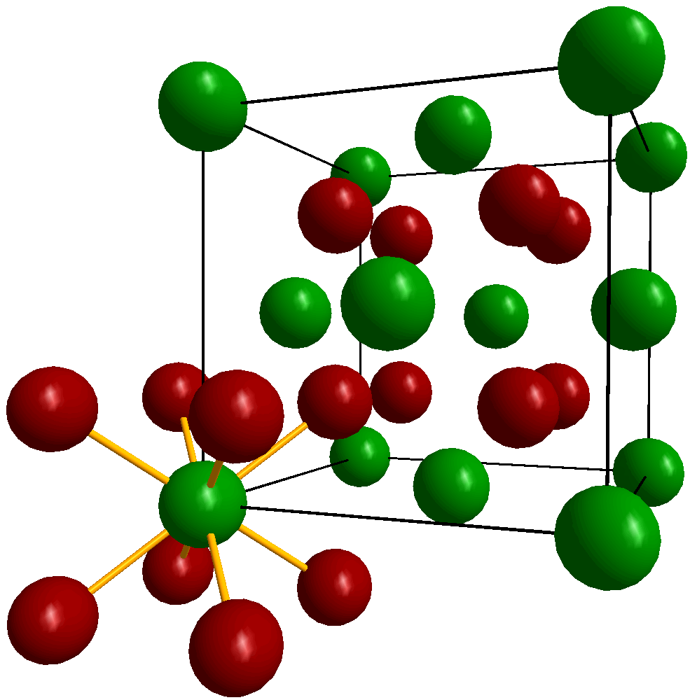
8.1 Introduction
UO2 is an ionic material and its \HyColor@XZeroOneThreeFour\pc@goptd@color\pc@hyenc@colorpdfcommentcolor\HyColor@XZeroOneThreeFour\pc@goptd@fontcolor\pc@hyenc@fontcolorpdfcommentcolor\HyColor@XZeroOneThreeFour\pc@goptd@icolor\pc@hyenc@icolorpdfcommentcolor\pdfmark[CF]pdfmark=/ANN,Subtype=/Widget,Raw=/TU (crystal field\textCR(\pc@goptd@deadline)) /T (tooltip zref@1955) /C [ ] /FT/Btn /F 768 /Ff 65536 /H/N /BS << /W 0 >> ground state has been fairly well determined with inelastic neutron scattering. Furthermore, it is cubic so that the number of \HyColor@XZeroOneThreeFour\pc@goptd@color\pc@hyenc@colorpdfcommentcolor\HyColor@XZeroOneThreeFour\pc@goptd@fontcolor\pc@hyenc@fontcolorpdfcommentcolor\HyColor@XZeroOneThreeFour\pc@goptd@icolor\pc@hyenc@icolorpdfcommentcolor\pdfmark[CF]pdfmark=/ANN,Subtype=/Widget,Raw=/TU (crystal field\textCR(\pc@goptd@deadline)) /T (tooltip zref@1956) /C [ ] /FT/Btn /F 768 /Ff 65536 /H/N /BS << /W 0 >> parameters is limited. It is therefore very interesting to use UO2 as a benchmark material for U, just like CeB6 for Ce, for testing the results obtained with \HyColor@XZeroOneThreeFour\pc@goptd@color\pc@hyenc@colorpdfcommentcolor\HyColor@XZeroOneThreeFour\pc@goptd@fontcolor\pc@hyenc@fontcolorpdfcommentcolor\HyColor@XZeroOneThreeFour\pc@goptd@icolor\pc@hyenc@icolorpdfcommentcolor\pdfmark[NIXS]pdfmark=/ANN,Subtype=/Widget,Raw=/TU (non-resonant inelastic x-ray scattering\textCR(\pc@goptd@deadline)) /T (tooltip zref@1957) /C [ ] /FT/Btn /F 768 /Ff 65536 /H/N /BS << /W 0 >> and Quanty [59, 60, 61].
Uranium dioxide is the most studied and most cited actinide material, as it is the nuclear fuel of most of the world’s reactors and a central material in the quest to understand radioactive waste and its interaction with the environment. The ground-state symmetry of uranium in UO2 has been discussed for many years. It was first proposed theoretically over 50 years ago. Numerous studies with neutron scattering have been interpreted with a triplet as the ground state.
The electronic 5 configuration has a 9-fold degenerate Hund’s rule ground state with total momentum = 4. In the cubic Oh point symmetry of UO2 the = 4 multiplet splits into one singlet , one doublet , and two triplets and . The representation of the \HyColor@XZeroOneThreeFour\pc@goptd@color\pc@hyenc@colorpdfcommentcolor\HyColor@XZeroOneThreeFour\pc@goptd@fontcolor\pc@hyenc@fontcolorpdfcommentcolor\HyColor@XZeroOneThreeFour\pc@goptd@icolor\pc@hyenc@icolorpdfcommentcolor\pdfmark[CF]pdfmark=/ANN,Subtype=/Widget,Raw=/TU (crystal field\textCR(\pc@goptd@deadline)) /T (tooltip zref@1958) /C [ ] /FT/Btn /F 768 /Ff 65536 /H/N /BS << /W 0 >> states is shown in Fig. 8.2.
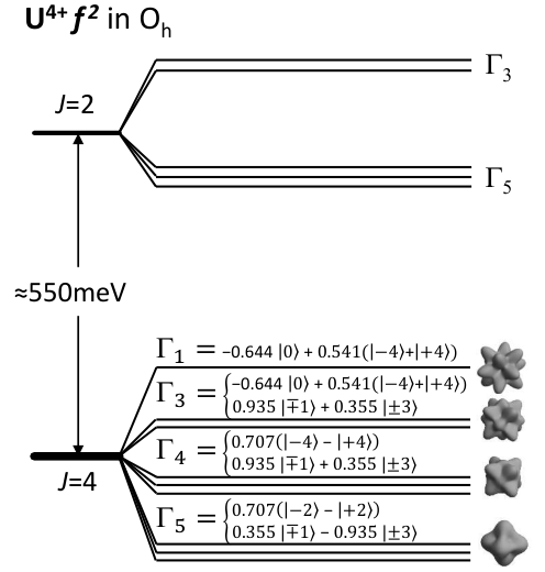
The first attempt to calculate the \HyColor@XZeroOneThreeFour\pc@goptd@color\pc@hyenc@colorpdfcommentcolor\HyColor@XZeroOneThreeFour\pc@goptd@fontcolor\pc@hyenc@fontcolorpdfcommentcolor\HyColor@XZeroOneThreeFour\pc@goptd@icolor\pc@hyenc@icolorpdfcommentcolor\pdfmark[CF]pdfmark=/ANN,Subtype=/Widget,Raw=/TU (crystal field\textCR(\pc@goptd@deadline)) /T (tooltip zref@1963) /C [ ] /FT/Btn /F 768 /Ff 65536 /H/N /BS << /W 0 >> ground state of UO2 was reported in 1966 [165]. By that time, the low-temperature antiferromagnetic moment was known approximately from neutron diffraction experiments [166, 167], and was measured more accurately later as 1.74(2) /U atom [168]. The energy levels of the \HyColor@XZeroOneThreeFour\pc@goptd@color\pc@hyenc@colorpdfcommentcolor\HyColor@XZeroOneThreeFour\pc@goptd@fontcolor\pc@hyenc@fontcolorpdfcommentcolor\HyColor@XZeroOneThreeFour\pc@goptd@icolor\pc@hyenc@icolorpdfcommentcolor\pdfmark[CF]pdfmark=/ANN,Subtype=/Widget,Raw=/TU (crystal field\textCR(\pc@goptd@deadline)) /T (tooltip zref@1964) /C [ ] /FT/Btn /F 768 /Ff 65536 /H/N /BS << /W 0 >> ground-state were measured with inelastic neutron scattering [169, 170]. More recently, a large number of experiments and theory have been performed on UO2 and are discussed in Ref. [19, 171, 172]. All of these studies take as a basic assumption that the \HyColor@XZeroOneThreeFour\pc@goptd@color\pc@hyenc@colorpdfcommentcolor\HyColor@XZeroOneThreeFour\pc@goptd@fontcolor\pc@hyenc@fontcolorpdfcommentcolor\HyColor@XZeroOneThreeFour\pc@goptd@icolor\pc@hyenc@icolorpdfcommentcolor\pdfmark[CF]pdfmark=/ANN,Subtype=/Widget,Raw=/TU (crystal field\textCR(\pc@goptd@deadline)) /T (tooltip zref@1965) /C [ ] /FT/Btn /F 768 /Ff 65536 /H/N /BS << /W 0 >> ground state is the triplet within the multiplet. Moreover, this ground state, given by the \HyColor@XZeroOneThreeFour\pc@goptd@color\pc@hyenc@colorpdfcommentcolor\HyColor@XZeroOneThreeFour\pc@goptd@fontcolor\pc@hyenc@fontcolorpdfcommentcolor\HyColor@XZeroOneThreeFour\pc@goptd@icolor\pc@hyenc@icolorpdfcommentcolor\pdfmark[CF]pdfmark=/ANN,Subtype=/Widget,Raw=/TU (crystal field\textCR(\pc@goptd@deadline)) /T (tooltip zref@1966) /C [ ] /FT/Btn /F 768 /Ff 65536 /H/N /BS << /W 0 >> parameters and in Stevens formalism, fits well with those determined for other light actinides, since and (scaled by the expectation values of the and operators over the appropriate 5-electron wave function) should be approximately independent of the actinide ion considered [173, 174]. and relate to the Wybourne formalism by and and the relations = and = are given by the Oh point symmetry (see App. D and Ref. [170]).
The 5 electrons are more delocalized than the 4 (see Fig. 3.2). As a result the \HyColor@XZeroOneThreeFour\pc@goptd@color\pc@hyenc@colorpdfcommentcolor\HyColor@XZeroOneThreeFour\pc@goptd@fontcolor\pc@hyenc@fontcolorpdfcommentcolor\HyColor@XZeroOneThreeFour\pc@goptd@icolor\pc@hyenc@icolorpdfcommentcolor\pdfmark[CF]pdfmark=/ANN,Subtype=/Widget,Raw=/TU (crystal field\textCR(\pc@goptd@deadline)) /T (tooltip zref@1967) /C [ ] /FT/Btn /F 768 /Ff 65536 /H/N /BS << /W 0 >> splittings are larger in uranium than in the rare earth and the magnetic intensities in a neutron spectrum are strongly broadened so that most uranium compounds do not exhibit sharp \HyColor@XZeroOneThreeFour\pc@goptd@color\pc@hyenc@colorpdfcommentcolor\HyColor@XZeroOneThreeFour\pc@goptd@fontcolor\pc@hyenc@fontcolorpdfcommentcolor\HyColor@XZeroOneThreeFour\pc@goptd@icolor\pc@hyenc@icolorpdfcommentcolor\pdfmark[CF]pdfmark=/ANN,Subtype=/Widget,Raw=/TU (crystal field\textCR(\pc@goptd@deadline)) /T (tooltip zref@1968) /C [ ] /FT/Btn /F 768 /Ff 65536 /H/N /BS << /W 0 >> excitations in neutron inelastic scattering [175]. There are only a few more localized exceptions like e.g. the oxide UO2 [170], the metallic UPd3 [176], or the semimetallic U3Pt3Sb4 [177]. Also in \HyColor@XZeroOneThreeFour\pc@goptd@color\pc@hyenc@colorpdfcommentcolor\HyColor@XZeroOneThreeFour\pc@goptd@fontcolor\pc@hyenc@fontcolorpdfcommentcolor\HyColor@XZeroOneThreeFour\pc@goptd@icolor\pc@hyenc@icolorpdfcommentcolor\pdfmark[XAS]pdfmark=/ANN,Subtype=/Widget,Raw=/TU (x-ray absorption spectroscopy\textCR(\pc@goptd@deadline)) /T (tooltip zref@1969) /C [ ] /FT/Btn /F 768 /Ff 65536 /H/N /BS << /W 0 >> the lines are strongly broadened and no multiplet structures have been observed in metallic uranium compounds [178].
8.2 Experimental
@goptd@color\pc@hyenc@colorpdfcommentcolor\HyColor@XZeroOneThreeFour\pc@goptd@fontcolor\pc@hyenc@fontcolorpdfcommentcolor\HyColor@XZeroOneThreeFour\pc@goptd@icolor\pc@hyenc@icolorpdfcommentcolor\pdfmark[NIXS]pdfmark=/ANN,Subtype=/Widget,Raw=/TU (non-resonant inelastic x-ray scattering\textCR(\pc@goptd@deadline)) /T (tooltip zref@1970) /C [ ] /FT/Btn /F 768 /Ff 65536 /H/N /BS << /W 0 >> data of UO2 had been taken by R. Caciuffo, G. Lander and G. van der Laan already in 2013, but had not been analyzed after several years. Here, we joined forces and the analysis of their data became part of this thesis.
The \HyColor@XZeroOneThreeFour\pc@goptd@color\pc@hyenc@colorpdfcommentcolor\HyColor@XZeroOneThreeFour\pc@goptd@fontcolor\pc@hyenc@fontcolorpdfcommentcolor\HyColor@XZeroOneThreeFour\pc@goptd@icolor\pc@hyenc@icolorpdfcommentcolor\pdfmark[NIXS]pdfmark=/ANN,Subtype=/Widget,Raw=/TU (non-resonant inelastic x-ray scattering\textCR(\pc@goptd@deadline)) /T (tooltip zref@1971) /C [ ] /FT/Btn /F 768 /Ff 65536 /H/N /BS << /W 0 >> experiment was performed with L. Simonelli at the Resonant Inelastic X-ray Spectrometer (RIXS) installed at the ID20 beamline of the European Synchrotron Radiation Facility, in Grenoble, France [179]. The incident beam with an intensity of 7 1013 photons/s and a 25 rad vertical divergence of the undulator radiation was generated by three consecutive undulators. It was monochromatized by a Si(111) double-crystal monochromator and horizontally focused by a Rh-coated mirror. Five spherically bent Si(660) analyzers were placed at scattering angles 2\HyColor@XZeroOneThreeFour\pc@goptd@color\pc@hyenc@colorpdfcommentcolor\HyColor@XZeroOneThreeFour\pc@goptd@fontcolor\pc@hyenc@fontcolorpdfcommentcolor\HyColor@XZeroOneThreeFour\pc@goptd@icolor\pc@hyenc@icolorpdfcommentcolor\pdfmark[]pdfmark=/ANN,Subtype=/Widget,Raw=/TU (scattering angle\textCR(\pc@goptd@deadline)) /T (tooltip zref@1972) /C [ ] /FT/Btn /F 768 /Ff 65536 /H/N /BS << /W 0 >> = 100, 110, 120, 130, and 140∘ on vertical Rowland circles. The fixed Bragg angle of \HyColor@XZeroOneThreeFour\pc@goptd@color\pc@hyenc@colorpdfcommentcolor\HyColor@XZeroOneThreeFour\pc@goptd@fontcolor\pc@hyenc@fontcolorpdfcommentcolor\HyColor@XZeroOneThreeFour\pc@goptd@icolor\pc@hyenc@icolorpdfcommentcolor\pdfmark[]pdfmark=/ANN,Subtype=/Widget,Raw=/TU (Bragg angle\textCR(\pc@goptd@deadline)) /T (tooltip zref@1973) /C [ ] /FT/Btn /F 768 /Ff 65536 /H/N /BS << /W 0 >> = 87.5∘ provides a resolution of 0.7 eV at a final photon energy \HyColor@XZeroOneThreeFour\pc@goptd@color\pc@hyenc@colorpdfcommentcolor\HyColor@XZeroOneThreeFour\pc@goptd@fontcolor\pc@hyenc@fontcolorpdfcommentcolor\HyColor@XZeroOneThreeFour\pc@goptd@icolor\pc@hyenc@icolorpdfcommentcolor\pdfmark[]pdfmark=/ANN,Subtype=/Widget,Raw=/TU (energy of the outgoing photon\textCR(\pc@goptd@deadline)) /T (tooltip zref@1974) /C [ ] /FT/Btn /F 768 /Ff 65536 /H/N /BS << /W 0 >> of 9.69 keV. The scattered intensity was recorded by a MAXIPIX fast readout, photon-counting position sensitive detector, achieving up to 1.4 kHz frame rate with 290 s readout dead time, with a pixel size of 55 m and a detection geometry of 256 256 pixels.
The samples are fully described in Ref. [180]. For the measurements two UO2 single crystals were cut and polished by Walt Ellis at Los Alamos National Laboratory [181]. One had the polished surface perpendicular to the \HyColor@XZeroOneThreeFour\pc@goptd@color\pc@hyenc@colorpdfcommentcolor\HyColor@XZeroOneThreeFour\pc@goptd@fontcolor\pc@hyenc@fontcolorpdfcommentcolor\HyColor@XZeroOneThreeFour\pc@goptd@icolor\pc@hyenc@icolorpdfcommentcolor\pdfmark[[111]]pdfmark=/ANN,Subtype=/Widget,Raw=/TU (direct lattice vector\textCR(\pc@goptd@deadline)) /T (tooltip zref@1975) /C [ ] /FT/Btn /F 768 /Ff 65536 /H/N /BS << /W 0 >> direction, the other to the \HyColor@XZeroOneThreeFour\pc@goptd@color\pc@hyenc@colorpdfcommentcolor\HyColor@XZeroOneThreeFour\pc@goptd@fontcolor\pc@hyenc@fontcolorpdfcommentcolor\HyColor@XZeroOneThreeFour\pc@goptd@icolor\pc@hyenc@icolorpdfcommentcolor\pdfmark[[100]]pdfmark=/ANN,Subtype=/Widget,Raw=/TU (direct lattice vector\textCR(\pc@goptd@deadline)) /T (tooltip zref@1976) /C [ ] /FT/Btn /F 768 /Ff 65536 /H/N /BS << /W 0 >> . The samples were aligned with the \HyColor@XZeroOneThreeFour\pc@goptd@color\pc@hyenc@colorpdfcommentcolor\HyColor@XZeroOneThreeFour\pc@goptd@fontcolor\pc@hyenc@fontcolorpdfcommentcolor\HyColor@XZeroOneThreeFour\pc@goptd@icolor\pc@hyenc@icolorpdfcommentcolor\pdfmark[[100]]pdfmark=/ANN,Subtype=/Widget,Raw=/TU (direct lattice vector\textCR(\pc@goptd@deadline)) /T (tooltip zref@1977) /C [ ] /FT/Btn /F 768 /Ff 65536 /H/N /BS << /W 0 >> and \HyColor@XZeroOneThreeFour\pc@goptd@color\pc@hyenc@colorpdfcommentcolor\HyColor@XZeroOneThreeFour\pc@goptd@fontcolor\pc@hyenc@fontcolorpdfcommentcolor\HyColor@XZeroOneThreeFour\pc@goptd@icolor\pc@hyenc@icolorpdfcommentcolor\pdfmark[[111]]pdfmark=/ANN,Subtype=/Widget,Raw=/TU (direct lattice vector\textCR(\pc@goptd@deadline)) /T (tooltip zref@1978) /C [ ] /FT/Btn /F 768 /Ff 65536 /H/N /BS << /W 0 >> surface normal for specular geometry with respect to the analyzer at 2\HyColor@XZeroOneThreeFour\pc@goptd@color\pc@hyenc@colorpdfcommentcolor\HyColor@XZeroOneThreeFour\pc@goptd@fontcolor\pc@hyenc@fontcolorpdfcommentcolor\HyColor@XZeroOneThreeFour\pc@goptd@icolor\pc@hyenc@icolorpdfcommentcolor\pdfmark[]pdfmark=/ANN,Subtype=/Widget,Raw=/TU (scattering angle\textCR(\pc@goptd@deadline)) /T (tooltip zref@1979) /C [ ] /FT/Btn /F 768 /Ff 65536 /H/N /BS << /W 0 >> = 120∘, i.e. pointing along = 60∘. The \HyColor@XZeroOneThreeFour\pc@goptd@color\pc@hyenc@colorpdfcommentcolor\HyColor@XZeroOneThreeFour\pc@goptd@fontcolor\pc@hyenc@fontcolorpdfcommentcolor\HyColor@XZeroOneThreeFour\pc@goptd@icolor\pc@hyenc@icolorpdfcommentcolor\pdfmark[[110]]pdfmark=/ANN,Subtype=/Widget,Raw=/TU (direct lattice vector\textCR(\pc@goptd@deadline)) /T (tooltip zref@1980) /C [ ] /FT/Btn /F 768 /Ff 65536 /H/N /BS << /W 0 >> direction was realized by rotating the \HyColor@XZeroOneThreeFour\pc@goptd@color\pc@hyenc@colorpdfcommentcolor\HyColor@XZeroOneThreeFour\pc@goptd@fontcolor\pc@hyenc@fontcolorpdfcommentcolor\HyColor@XZeroOneThreeFour\pc@goptd@icolor\pc@hyenc@icolorpdfcommentcolor\pdfmark[[100]]pdfmark=/ANN,Subtype=/Widget,Raw=/TU (direct lattice vector\textCR(\pc@goptd@deadline)) /T (tooltip zref@1981) /C [ ] /FT/Btn /F 768 /Ff 65536 /H/N /BS << /W 0 >> crystal accordingly. \HyColor@XZeroOneThreeFour\pc@goptd@color\pc@hyenc@colorpdfcommentcolor\HyColor@XZeroOneThreeFour\pc@goptd@fontcolor\pc@hyenc@fontcolorpdfcommentcolor\HyColor@XZeroOneThreeFour\pc@goptd@icolor\pc@hyenc@icolorpdfcommentcolor\pdfmark[NIXS]pdfmark=/ANN,Subtype=/Widget,Raw=/TU (non-resonant inelastic x-ray scattering\textCR(\pc@goptd@deadline)) /T (tooltip zref@1982) /C [ ] /FT/Btn /F 768 /Ff 65536 /H/N /BS << /W 0 >> data of the UO2 \HyColor@XZeroOneThreeFour\pc@goptd@color\pc@hyenc@colorpdfcommentcolor\HyColor@XZeroOneThreeFour\pc@goptd@fontcolor\pc@hyenc@fontcolorpdfcommentcolor\HyColor@XZeroOneThreeFour\pc@goptd@icolor\pc@hyenc@icolorpdfcommentcolor\pdfmark[U O4,5]pdfmark=/ANN,Subtype=/Widget,Raw=/TU (absorption edge\textCR(\pc@goptd@deadline)) /T (tooltip zref@1983) /C [ ] /FT/Btn /F 768 /Ff 65536 /H/N /BS << /W 0 >> edges () were measured at room temperature.
For data analysis, only data collected in the highest analyzer at 2\HyColor@XZeroOneThreeFour\pc@goptd@color\pc@hyenc@colorpdfcommentcolor\HyColor@XZeroOneThreeFour\pc@goptd@fontcolor\pc@hyenc@fontcolorpdfcommentcolor\HyColor@XZeroOneThreeFour\pc@goptd@icolor\pc@hyenc@icolorpdfcommentcolor\pdfmark[]pdfmark=/ANN,Subtype=/Widget,Raw=/TU (scattering angle\textCR(\pc@goptd@deadline)) /T (tooltip zref@1984) /C [ ] /FT/Btn /F 768 /Ff 65536 /H/N /BS << /W 0 >> = 140∘, which also had the largest intensity in the horizontal scattering geometry, were used because here the momentum transfer is largest. The corresponding momentum transfer \HyColor@XZeroOneThreeFour\pc@goptd@color\pc@hyenc@colorpdfcommentcolor\HyColor@XZeroOneThreeFour\pc@goptd@fontcolor\pc@hyenc@fontcolorpdfcommentcolor\HyColor@XZeroOneThreeFour\pc@goptd@icolor\pc@hyenc@icolorpdfcommentcolor\pdfmark[]pdfmark=/ANN,Subtype=/Widget,Raw=/TU (momentum transfer\textCR(\pc@goptd@deadline)) /T (tooltip zref@1985) /C [ ] /FT/Btn /F 768 /Ff 65536 /H/N /BS << /W 0 >> at the elastic energy at \HyColor@XZeroOneThreeFour\pc@goptd@color\pc@hyenc@colorpdfcommentcolor\HyColor@XZeroOneThreeFour\pc@goptd@fontcolor\pc@hyenc@fontcolorpdfcommentcolor\HyColor@XZeroOneThreeFour\pc@goptd@icolor\pc@hyenc@icolorpdfcommentcolor\pdfmark[]pdfmark=/ANN,Subtype=/Widget,Raw=/TU (scattering angle\textCR(\pc@goptd@deadline)) /T (tooltip zref@1986) /C [ ] /FT/Btn /F 768 /Ff 65536 /H/N /BS << /W 0 >> = 70∘ amounts to |\HyColor@XZeroOneThreeFour\pc@goptd@color\pc@hyenc@colorpdfcommentcolor\HyColor@XZeroOneThreeFour\pc@goptd@fontcolor\pc@hyenc@fontcolorpdfcommentcolor\HyColor@XZeroOneThreeFour\pc@goptd@icolor\pc@hyenc@icolorpdfcommentcolor\pdfmark[]pdfmark=/ANN,Subtype=/Widget,Raw=/TU (momentum transfer\textCR(\pc@goptd@deadline)) /T (tooltip zref@1987) /C [ ] /FT/Btn /F 768 /Ff 65536 /H/N /BS << /W 0 >> | = 9.1 Å-1. Note, that there is an offset of 10∘ between the respective crystallographic directions which were aligned at = 60∘ and \HyColor@XZeroOneThreeFour\pc@goptd@color\pc@hyenc@colorpdfcommentcolor\HyColor@XZeroOneThreeFour\pc@goptd@fontcolor\pc@hyenc@fontcolorpdfcommentcolor\HyColor@XZeroOneThreeFour\pc@goptd@icolor\pc@hyenc@icolorpdfcommentcolor\pdfmark[]pdfmark=/ANN,Subtype=/Widget,Raw=/TU (momentum transfer\textCR(\pc@goptd@deadline)) /T (tooltip zref@1988) /C [ ] /FT/Btn /F 768 /Ff 65536 /H/N /BS << /W 0 >> . This has been taken into account when analyzing the data.
8.3 NIXS results
| \HyColor@XZeroOneThreeFour\pc@goptd@color\pc@hyenc@colorpdfcommentcolor\HyColor@XZeroOneThreeFour\pc@goptd@fontcolor\pc@hyenc@fontcolorpdfcommentcolor\HyColor@XZeroOneThreeFour\pc@goptd@icolor\pc@hyenc@icolorpdfcommentcolor\pdfmark[redff]pdfmark=/ANN,Subtype=/Widget,Raw=/TU (scaling of the valence-valence Coulomb interaction\textCR(\pc@goptd@deadline)) /T (tooltip zref@1989) /C [ ] /FT/Btn /F 768 /Ff 65536 /H/N /BS << /W 0 >> | \HyColor@XZeroOneThreeFour\pc@goptd@color\pc@hyenc@colorpdfcommentcolor\HyColor@XZeroOneThreeFour\pc@goptd@fontcolor\pc@hyenc@fontcolorpdfcommentcolor\HyColor@XZeroOneThreeFour\pc@goptd@icolor\pc@hyenc@icolorpdfcommentcolor\pdfmark[redfc]pdfmark=/ANN,Subtype=/Widget,Raw=/TU (scaling of the core-valence Coulomb interaction\textCR(\pc@goptd@deadline)) /T (tooltip zref@1990) /C [ ] /FT/Btn /F 768 /Ff 65536 /H/N /BS << /W 0 >> | \HyColor@XZeroOneThreeFour\pc@goptd@color\pc@hyenc@colorpdfcommentcolor\HyColor@XZeroOneThreeFour\pc@goptd@fontcolor\pc@hyenc@fontcolorpdfcommentcolor\HyColor@XZeroOneThreeFour\pc@goptd@icolor\pc@hyenc@icolorpdfcommentcolor\pdfmark[red]pdfmark=/ANN,Subtype=/Widget,Raw=/TU (scaling of the core spin-orbit coupling\textCR(\pc@goptd@deadline)) /T (tooltip zref@1991) /C [ ] /FT/Btn /F 768 /Ff 65536 /H/N /BS << /W 0 >> | \HyColor@XZeroOneThreeFour\pc@goptd@color\pc@hyenc@colorpdfcommentcolor\HyColor@XZeroOneThreeFour\pc@goptd@fontcolor\pc@hyenc@fontcolorpdfcommentcolor\HyColor@XZeroOneThreeFour\pc@goptd@icolor\pc@hyenc@icolorpdfcommentcolor\pdfmark[red]pdfmark=/ANN,Subtype=/Widget,Raw=/TU (scaling of the valence spin-orbit coupling\textCR(\pc@goptd@deadline)) /T (tooltip zref@1992) /C [ ] /FT/Btn /F 768 /Ff 65536 /H/N /BS << /W 0 >> | |\HyColor@XZeroOneThreeFour\pc@goptd@color\pc@hyenc@colorpdfcommentcolor\HyColor@XZeroOneThreeFour\pc@goptd@fontcolor\pc@hyenc@fontcolorpdfcommentcolor\HyColor@XZeroOneThreeFour\pc@goptd@icolor\pc@hyenc@icolorpdfcommentcolor\pdfmark[]pdfmark=/ANN,Subtype=/Widget,Raw=/TU (momentum transfer\textCR(\pc@goptd@deadline)) /T (tooltip zref@1993) /C [ ] /FT/Btn /F 768 /Ff 65536 /H/N /BS << /W 0 >> |/ | \HyColor@XZeroOneThreeFour\pc@goptd@color\pc@hyenc@colorpdfcommentcolor\HyColor@XZeroOneThreeFour\pc@goptd@fontcolor\pc@hyenc@fontcolorpdfcommentcolor\HyColor@XZeroOneThreeFour\pc@goptd@icolor\pc@hyenc@icolorpdfcommentcolor\pdfmark[FWHML]pdfmark=/ANN,Subtype=/Widget,Raw=/TU (Lorentzian full width at half maximum\textCR(\pc@goptd@deadline)) /T (tooltip zref@1994) /C [ ] /FT/Btn /F 768 /Ff 65536 /H/N /BS << /W 0 >> | \HyColor@XZeroOneThreeFour\pc@goptd@color\pc@hyenc@colorpdfcommentcolor\HyColor@XZeroOneThreeFour\pc@goptd@fontcolor\pc@hyenc@fontcolorpdfcommentcolor\HyColor@XZeroOneThreeFour\pc@goptd@icolor\pc@hyenc@icolorpdfcommentcolor\pdfmark[FWHMG]pdfmark=/ANN,Subtype=/Widget,Raw=/TU (Gaussian full width at half maximum\textCR(\pc@goptd@deadline)) /T (tooltip zref@1995) /C [ ] /FT/Btn /F 768 /Ff 65536 /H/N /BS << /W 0 >> |
|---|---|---|---|---|---|---|
| 0.6 (1) | 0.6 (1) | 1.00 (5) | 1.00 (5) | 9.4 (2) | 0.6 (2) eV | 0.65 eV |
Figure 8.3a shows the UO2 \HyColor@XZeroOneThreeFour\pc@goptd@color\pc@hyenc@colorpdfcommentcolor\HyColor@XZeroOneThreeFour\pc@goptd@fontcolor\pc@hyenc@fontcolorpdfcommentcolor\HyColor@XZeroOneThreeFour\pc@goptd@icolor\pc@hyenc@icolorpdfcommentcolor\pdfmark[NIXS]pdfmark=/ANN,Subtype=/Widget,Raw=/TU (non-resonant inelastic x-ray scattering\textCR(\pc@goptd@deadline)) /T (tooltip zref@2002) /C [ ] /FT/Btn /F 768 /Ff 65536 /H/N /BS << /W 0 >> spectrum for 9.1 over a large energy range. The three measured directions \HyColor@XZeroOneThreeFour\pc@goptd@color\pc@hyenc@colorpdfcommentcolor\HyColor@XZeroOneThreeFour\pc@goptd@fontcolor\pc@hyenc@fontcolorpdfcommentcolor\HyColor@XZeroOneThreeFour\pc@goptd@icolor\pc@hyenc@icolorpdfcommentcolor\pdfmark[]pdfmark=/ANN,Subtype=/Widget,Raw=/TU (momentum transfer\textCR(\pc@goptd@deadline)) /T (tooltip zref@2003) /C [ ] /FT/Btn /F 768 /Ff 65536 /H/N /BS << /W 0 >> || \HyColor@XZeroOneThreeFour\pc@goptd@color\pc@hyenc@colorpdfcommentcolor\HyColor@XZeroOneThreeFour\pc@goptd@fontcolor\pc@hyenc@fontcolorpdfcommentcolor\HyColor@XZeroOneThreeFour\pc@goptd@icolor\pc@hyenc@icolorpdfcommentcolor\pdfmark[[100]]pdfmark=/ANN,Subtype=/Widget,Raw=/TU (direct lattice vector\textCR(\pc@goptd@deadline)) /T (tooltip zref@2004) /C [ ] /FT/Btn /F 768 /Ff 65536 /H/N /BS << /W 0 >> , \HyColor@XZeroOneThreeFour\pc@goptd@color\pc@hyenc@colorpdfcommentcolor\HyColor@XZeroOneThreeFour\pc@goptd@fontcolor\pc@hyenc@fontcolorpdfcommentcolor\HyColor@XZeroOneThreeFour\pc@goptd@icolor\pc@hyenc@icolorpdfcommentcolor\pdfmark[]pdfmark=/ANN,Subtype=/Widget,Raw=/TU (momentum transfer\textCR(\pc@goptd@deadline)) /T (tooltip zref@2005) /C [ ] /FT/Btn /F 768 /Ff 65536 /H/N /BS << /W 0 >> || \HyColor@XZeroOneThreeFour\pc@goptd@color\pc@hyenc@colorpdfcommentcolor\HyColor@XZeroOneThreeFour\pc@goptd@fontcolor\pc@hyenc@fontcolorpdfcommentcolor\HyColor@XZeroOneThreeFour\pc@goptd@icolor\pc@hyenc@icolorpdfcommentcolor\pdfmark[[110]]pdfmark=/ANN,Subtype=/Widget,Raw=/TU (direct lattice vector\textCR(\pc@goptd@deadline)) /T (tooltip zref@2006) /C [ ] /FT/Btn /F 768 /Ff 65536 /H/N /BS << /W 0 >> , and \HyColor@XZeroOneThreeFour\pc@goptd@color\pc@hyenc@colorpdfcommentcolor\HyColor@XZeroOneThreeFour\pc@goptd@fontcolor\pc@hyenc@fontcolorpdfcommentcolor\HyColor@XZeroOneThreeFour\pc@goptd@icolor\pc@hyenc@icolorpdfcommentcolor\pdfmark[]pdfmark=/ANN,Subtype=/Widget,Raw=/TU (momentum transfer\textCR(\pc@goptd@deadline)) /T (tooltip zref@2007) /C [ ] /FT/Btn /F 768 /Ff 65536 /H/N /BS << /W 0 >> || \HyColor@XZeroOneThreeFour\pc@goptd@color\pc@hyenc@colorpdfcommentcolor\HyColor@XZeroOneThreeFour\pc@goptd@fontcolor\pc@hyenc@fontcolorpdfcommentcolor\HyColor@XZeroOneThreeFour\pc@goptd@icolor\pc@hyenc@icolorpdfcommentcolor\pdfmark[[111]]pdfmark=/ANN,Subtype=/Widget,Raw=/TU (direct lattice vector\textCR(\pc@goptd@deadline)) /T (tooltip zref@2008) /C [ ] /FT/Btn /F 768 /Ff 65536 /H/N /BS << /W 0 >> have been added up in order to improve the statistics. Each direction has a integration time of 10 s per point. The \HyColor@XZeroOneThreeFour\pc@goptd@color\pc@hyenc@colorpdfcommentcolor\HyColor@XZeroOneThreeFour\pc@goptd@fontcolor\pc@hyenc@fontcolorpdfcommentcolor\HyColor@XZeroOneThreeFour\pc@goptd@icolor\pc@hyenc@icolorpdfcommentcolor\pdfmark[U O]pdfmark=/ANN,Subtype=/Widget,Raw=/TU (absorption edge\textCR(\pc@goptd@deadline)) /T (tooltip zref@2009) /C [ ] /FT/Btn /F 768 /Ff 65536 /H/N /BS << /W 0 >> edges can be seen distinctly on top of the broad Compton background that peaks at about 300 eV. Here, the \HyColor@XZeroOneThreeFour\pc@goptd@color\pc@hyenc@colorpdfcommentcolor\HyColor@XZeroOneThreeFour\pc@goptd@fontcolor\pc@hyenc@fontcolorpdfcommentcolor\HyColor@XZeroOneThreeFour\pc@goptd@icolor\pc@hyenc@icolorpdfcommentcolor\pdfmark[U O4,5]pdfmark=/ANN,Subtype=/Widget,Raw=/TU (absorption edge\textCR(\pc@goptd@deadline)) /T (tooltip zref@2010) /C [ ] /FT/Btn /F 768 /Ff 65536 /H/N /BS << /W 0 >> edges () is the most suited edge for studying the uranium 5 wave function. It is the strongest and has the best signal to background ratio of all visible U core levels, just as the rare-earth \HyColor@XZeroOneThreeFour\pc@goptd@color\pc@hyenc@colorpdfcommentcolor\HyColor@XZeroOneThreeFour\pc@goptd@fontcolor\pc@hyenc@fontcolorpdfcommentcolor\HyColor@XZeroOneThreeFour\pc@goptd@icolor\pc@hyenc@icolorpdfcommentcolor\pdfmark[RE N4,5]pdfmark=/ANN,Subtype=/Widget,Raw=/TU (absorption edge\textCR(\pc@goptd@deadline)) /T (tooltip zref@2011) /C [ ] /FT/Btn /F 768 /Ff 65536 /H/N /BS << /W 0 >> edges (). The huge intensity around 500 eV is only present in the data of one direction and cannot arise form a core level, instead it is likely due to some Bragg scattering that reached the detector without passing the analyzer. Such signals are referred to as spurious scattering.
Multiplet structure
Figure 8.3b shows the pseudo-isotropic spectrum of the \HyColor@XZeroOneThreeFour\pc@goptd@color\pc@hyenc@colorpdfcommentcolor\HyColor@XZeroOneThreeFour\pc@goptd@fontcolor\pc@hyenc@fontcolorpdfcommentcolor\HyColor@XZeroOneThreeFour\pc@goptd@icolor\pc@hyenc@icolorpdfcommentcolor\pdfmark[U O4,5]pdfmark=/ANN,Subtype=/Widget,Raw=/TU (absorption edge\textCR(\pc@goptd@deadline)) /T (tooltip zref@2012) /C [ ] /FT/Btn /F 768 /Ff 65536 /H/N /BS << /W 0 >> edges with energy steps of 0.2 eV and an integration time of 6 min/point per direction. The pseudo-isotropic spectrum is the same linear combination of the three measured directions as in Eq. 5.1 for CeB6, which is isotropic for the \HyColor@XZeroOneThreeFour\pc@goptd@color\pc@hyenc@colorpdfcommentcolor\HyColor@XZeroOneThreeFour\pc@goptd@fontcolor\pc@hyenc@fontcolorpdfcommentcolor\HyColor@XZeroOneThreeFour\pc@goptd@icolor\pc@hyenc@icolorpdfcommentcolor\pdfmark[k]pdfmark=/ANN,Subtype=/Widget,Raw=/TU (multipolar order\textCR(\pc@goptd@deadline)) /T (tooltip zref@2013) /C [ ] /FT/Btn /F 768 /Ff 65536 /H/N /BS << /W 0 >> = 3 transition but not for \HyColor@XZeroOneThreeFour\pc@goptd@color\pc@hyenc@colorpdfcommentcolor\HyColor@XZeroOneThreeFour\pc@goptd@fontcolor\pc@hyenc@fontcolorpdfcommentcolor\HyColor@XZeroOneThreeFour\pc@goptd@icolor\pc@hyenc@icolorpdfcommentcolor\pdfmark[k]pdfmark=/ANN,Subtype=/Widget,Raw=/TU (multipolar order\textCR(\pc@goptd@deadline)) /T (tooltip zref@2014) /C [ ] /FT/Btn /F 768 /Ff 65536 /H/N /BS << /W 0 >> = 5. The black line represents the calculated isotropic spectrum. The \HyColor@XZeroOneThreeFour\pc@goptd@color\pc@hyenc@colorpdfcommentcolor\HyColor@XZeroOneThreeFour\pc@goptd@fontcolor\pc@hyenc@fontcolorpdfcommentcolor\HyColor@XZeroOneThreeFour\pc@goptd@icolor\pc@hyenc@icolorpdfcommentcolor\pdfmark[CF]pdfmark=/ANN,Subtype=/Widget,Raw=/TU (crystal field\textCR(\pc@goptd@deadline)) /T (tooltip zref@2015) /C [ ] /FT/Btn /F 768 /Ff 65536 /H/N /BS << /W 0 >> splitting has been neglected at this point. The atomic Coulomb interactions have been reduced to fit the observed peak positions. The instrumental Gaussian line width \HyColor@XZeroOneThreeFour\pc@goptd@color\pc@hyenc@colorpdfcommentcolor\HyColor@XZeroOneThreeFour\pc@goptd@fontcolor\pc@hyenc@fontcolorpdfcommentcolor\HyColor@XZeroOneThreeFour\pc@goptd@icolor\pc@hyenc@icolorpdfcommentcolor\pdfmark[FWHMG]pdfmark=/ANN,Subtype=/Widget,Raw=/TU (Gaussian full width at half maximum\textCR(\pc@goptd@deadline)) /T (tooltip zref@2016) /C [ ] /FT/Btn /F 768 /Ff 65536 /H/N /BS << /W 0 >> is determined by the elastic width and the Lorentzian lifetime broadening with width \HyColor@XZeroOneThreeFour\pc@goptd@color\pc@hyenc@colorpdfcommentcolor\HyColor@XZeroOneThreeFour\pc@goptd@fontcolor\pc@hyenc@fontcolorpdfcommentcolor\HyColor@XZeroOneThreeFour\pc@goptd@icolor\pc@hyenc@icolorpdfcommentcolor\pdfmark[FWHML]pdfmark=/ANN,Subtype=/Widget,Raw=/TU (Lorentzian full width at half maximum\textCR(\pc@goptd@deadline)) /T (tooltip zref@2017) /C [ ] /FT/Btn /F 768 /Ff 65536 /H/N /BS << /W 0 >> has been obtained by fitting the spectrum. The momentum transfer |\HyColor@XZeroOneThreeFour\pc@goptd@color\pc@hyenc@colorpdfcommentcolor\HyColor@XZeroOneThreeFour\pc@goptd@fontcolor\pc@hyenc@fontcolorpdfcommentcolor\HyColor@XZeroOneThreeFour\pc@goptd@icolor\pc@hyenc@icolorpdfcommentcolor\pdfmark[]pdfmark=/ANN,Subtype=/Widget,Raw=/TU (momentum transfer\textCR(\pc@goptd@deadline)) /T (tooltip zref@2018) /C [ ] /FT/Btn /F 768 /Ff 65536 /H/N /BS << /W 0 >> | has been adjusted by fitting the isotropic spectrum. The final values are given in Tab. 8.1. The Hund’s rule ground state of the initial state with these values can be expressed by the linear combination of the term symbols with \HyColor@XZeroOneThreeFour\pc@goptd@color\pc@hyenc@colorpdfcommentcolor\HyColor@XZeroOneThreeFour\pc@goptd@fontcolor\pc@hyenc@fontcolorpdfcommentcolor\HyColor@XZeroOneThreeFour\pc@goptd@icolor\pc@hyenc@icolorpdfcommentcolor\pdfmark[J]pdfmark=/ANN,Subtype=/Widget,Raw=/TU (total momentum\textCR(\pc@goptd@deadline)) /T (tooltip zref@2019) /C [ ] /FT/Btn /F 768 /Ff 65536 /H/N /BS << /W 0 >> = 4:
| (8.1) |
The three sharp features at 94 eV, 98 eV, and 104 eV energy transfer, which are important for the \HyColor@XZeroOneThreeFour\pc@goptd@color\pc@hyenc@colorpdfcommentcolor\HyColor@XZeroOneThreeFour\pc@goptd@fontcolor\pc@hyenc@fontcolorpdfcommentcolor\HyColor@XZeroOneThreeFour\pc@goptd@icolor\pc@hyenc@icolorpdfcommentcolor\pdfmark[CF]pdfmark=/ANN,Subtype=/Widget,Raw=/TU (crystal field\textCR(\pc@goptd@deadline)) /T (tooltip zref@2023) /C [ ] /FT/Btn /F 768 /Ff 65536 /H/N /BS << /W 0 >> analysis in the regime of higher multiplet transitions, are already described in great detail by the simple model neglecting the \HyColor@XZeroOneThreeFour\pc@goptd@color\pc@hyenc@colorpdfcommentcolor\HyColor@XZeroOneThreeFour\pc@goptd@fontcolor\pc@hyenc@fontcolorpdfcommentcolor\HyColor@XZeroOneThreeFour\pc@goptd@icolor\pc@hyenc@icolorpdfcommentcolor\pdfmark[CF]pdfmark=/ANN,Subtype=/Widget,Raw=/TU (crystal field\textCR(\pc@goptd@deadline)) /T (tooltip zref@2024) /C [ ] /FT/Btn /F 768 /Ff 65536 /H/N /BS << /W 0 >> splitting. The most significant deviation between experiment and calculation is the additional intensity above 108 eV in the calculation. This may have two reasons as for the Ce/Sm edge in the hexaborides. The dipole dominated region is shifted due to a stronger reduced G1 Slater integral and/or the lines above 108 eV have a much larger lifetime broadening due to the vicinity to the continuum states. For UO2 no extra reduction of the Coulomb dipole interaction term (G1 Slater integral) was found that improves the fit significantly. The precise description of the dipole regime, would require the inclusion of the interaction with the continuum states and make the model much more complicated, with only a minor gain for the following analysis.
For finite Coulomb and spin-orbit coupling the total momentum of \HyColor@XZeroOneThreeFour\pc@goptd@color\pc@hyenc@colorpdfcommentcolor\HyColor@XZeroOneThreeFour\pc@goptd@fontcolor\pc@hyenc@fontcolorpdfcommentcolor\HyColor@XZeroOneThreeFour\pc@goptd@icolor\pc@hyenc@icolorpdfcommentcolor\pdfmark[J]pdfmark=/ANN,Subtype=/Widget,Raw=/TU (total momentum\textCR(\pc@goptd@deadline)) /T (tooltip zref@2025) /C [ ] /FT/Btn /F 768 /Ff 65536 /H/N /BS << /W 0 >> = 4 always forms the ground state. Figure 8.4 shows the energy level diagram for the U4+ 5 configuration as function of the Coulomb reduction factor \HyColor@XZeroOneThreeFour\pc@goptd@color\pc@hyenc@colorpdfcommentcolor\HyColor@XZeroOneThreeFour\pc@goptd@fontcolor\pc@hyenc@fontcolorpdfcommentcolor\HyColor@XZeroOneThreeFour\pc@goptd@icolor\pc@hyenc@icolorpdfcommentcolor\pdfmark[redff]pdfmark=/ANN,Subtype=/Widget,Raw=/TU (scaling of the valence-valence Coulomb interaction\textCR(\pc@goptd@deadline)) /T (tooltip zref@2026) /C [ ] /FT/Btn /F 768 /Ff 65536 /H/N /BS << /W 0 >> without considering a finite \HyColor@XZeroOneThreeFour\pc@goptd@color\pc@hyenc@colorpdfcommentcolor\HyColor@XZeroOneThreeFour\pc@goptd@fontcolor\pc@hyenc@fontcolorpdfcommentcolor\HyColor@XZeroOneThreeFour\pc@goptd@icolor\pc@hyenc@icolorpdfcommentcolor\pdfmark[CF]pdfmark=/ANN,Subtype=/Widget,Raw=/TU (crystal field\textCR(\pc@goptd@deadline)) /T (tooltip zref@2027) /C [ ] /FT/Btn /F 768 /Ff 65536 /H/N /BS << /W 0 >> potential. \HyColor@XZeroOneThreeFour\pc@goptd@color\pc@hyenc@colorpdfcommentcolor\HyColor@XZeroOneThreeFour\pc@goptd@fontcolor\pc@hyenc@fontcolorpdfcommentcolor\HyColor@XZeroOneThreeFour\pc@goptd@icolor\pc@hyenc@icolorpdfcommentcolor\pdfmark[redfc]pdfmark=/ANN,Subtype=/Widget,Raw=/TU (scaling of the core-valence Coulomb interaction\textCR(\pc@goptd@deadline)) /T (tooltip zref@2028) /C [ ] /FT/Btn /F 768 /Ff 65536 /H/N /BS << /W 0 >> does not contribute since only the initial state eigenvalues are shown. The gray range indicates the range that describes the UO2 \HyColor@XZeroOneThreeFour\pc@goptd@color\pc@hyenc@colorpdfcommentcolor\HyColor@XZeroOneThreeFour\pc@goptd@fontcolor\pc@hyenc@fontcolorpdfcommentcolor\HyColor@XZeroOneThreeFour\pc@goptd@icolor\pc@hyenc@icolorpdfcommentcolor\pdfmark[NIXS]pdfmark=/ANN,Subtype=/Widget,Raw=/TU (non-resonant inelastic x-ray scattering\textCR(\pc@goptd@deadline)) /T (tooltip zref@2029) /C [ ] /FT/Btn /F 768 /Ff 65536 /H/N /BS << /W 0 >> data best. It turns out that the calculated \HyColor@XZeroOneThreeFour\pc@goptd@color\pc@hyenc@colorpdfcommentcolor\HyColor@XZeroOneThreeFour\pc@goptd@fontcolor\pc@hyenc@fontcolorpdfcommentcolor\HyColor@XZeroOneThreeFour\pc@goptd@icolor\pc@hyenc@icolorpdfcommentcolor\pdfmark[J]pdfmark=/ANN,Subtype=/Widget,Raw=/TU (total momentum\textCR(\pc@goptd@deadline)) /T (tooltip zref@2030) /C [ ] /FT/Btn /F 768 /Ff 65536 /H/N /BS << /W 0 >> multiplet splittings within the applicable range of \HyColor@XZeroOneThreeFour\pc@goptd@color\pc@hyenc@colorpdfcommentcolor\HyColor@XZeroOneThreeFour\pc@goptd@fontcolor\pc@hyenc@fontcolorpdfcommentcolor\HyColor@XZeroOneThreeFour\pc@goptd@icolor\pc@hyenc@icolorpdfcommentcolor\pdfmark[redff]pdfmark=/ANN,Subtype=/Widget,Raw=/TU (scaling of the valence-valence Coulomb interaction\textCR(\pc@goptd@deadline)) /T (tooltip zref@2031) /C [ ] /FT/Btn /F 768 /Ff 65536 /H/N /BS << /W 0 >> match fairly well excitations seen by high resolution (160 meV) \HyColor@XZeroOneThreeFour\pc@goptd@color\pc@hyenc@colorpdfcommentcolor\HyColor@XZeroOneThreeFour\pc@goptd@fontcolor\pc@hyenc@fontcolorpdfcommentcolor\HyColor@XZeroOneThreeFour\pc@goptd@icolor\pc@hyenc@icolorpdfcommentcolor\pdfmark[RIXS]pdfmark=/ANN,Subtype=/Widget,Raw=/TU (resonant inelastic x-ray scattering\textCR(\pc@goptd@deadline)) /T (tooltip zref@2032) /C [ ] /FT/Btn /F 768 /Ff 65536 /H/N /BS << /W 0 >> at the \HyColor@XZeroOneThreeFour\pc@goptd@color\pc@hyenc@colorpdfcommentcolor\HyColor@XZeroOneThreeFour\pc@goptd@fontcolor\pc@hyenc@fontcolorpdfcommentcolor\HyColor@XZeroOneThreeFour\pc@goptd@icolor\pc@hyenc@icolorpdfcommentcolor\pdfmark[U O4,5]pdfmark=/ANN,Subtype=/Widget,Raw=/TU (absorption edge\textCR(\pc@goptd@deadline)) /T (tooltip zref@2033) /C [ ] /FT/Btn /F 768 /Ff 65536 /H/N /BS << /W 0 >> edges [182], shown by the data points in Figure 8.4. The best agreement with the multiplet lines is around \HyColor@XZeroOneThreeFour\pc@goptd@color\pc@hyenc@colorpdfcommentcolor\HyColor@XZeroOneThreeFour\pc@goptd@fontcolor\pc@hyenc@fontcolorpdfcommentcolor\HyColor@XZeroOneThreeFour\pc@goptd@icolor\pc@hyenc@icolorpdfcommentcolor\pdfmark[redff]pdfmark=/ANN,Subtype=/Widget,Raw=/TU (scaling of the valence-valence Coulomb interaction\textCR(\pc@goptd@deadline)) /T (tooltip zref@2034) /C [ ] /FT/Btn /F 768 /Ff 65536 /H/N /BS << /W 0 >> = 0.6-0.7. Note, this comparison not only lacks the assumption of a \HyColor@XZeroOneThreeFour\pc@goptd@color\pc@hyenc@colorpdfcommentcolor\HyColor@XZeroOneThreeFour\pc@goptd@fontcolor\pc@hyenc@fontcolorpdfcommentcolor\HyColor@XZeroOneThreeFour\pc@goptd@icolor\pc@hyenc@icolorpdfcommentcolor\pdfmark[CF]pdfmark=/ANN,Subtype=/Widget,Raw=/TU (crystal field\textCR(\pc@goptd@deadline)) /T (tooltip zref@2035) /C [ ] /FT/Btn /F 768 /Ff 65536 /H/N /BS << /W 0 >> splitting; it also does not take the core hole into account, which is absent in the \HyColor@XZeroOneThreeFour\pc@goptd@color\pc@hyenc@colorpdfcommentcolor\HyColor@XZeroOneThreeFour\pc@goptd@fontcolor\pc@hyenc@fontcolorpdfcommentcolor\HyColor@XZeroOneThreeFour\pc@goptd@icolor\pc@hyenc@icolorpdfcommentcolor\pdfmark[RIXS]pdfmark=/ANN,Subtype=/Widget,Raw=/TU (resonant inelastic x-ray scattering\textCR(\pc@goptd@deadline)) /T (tooltip zref@2036) /C [ ] /FT/Btn /F 768 /Ff 65536 /H/N /BS << /W 0 >> final state.
q -directional dependence
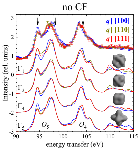
Figure 8.5 shows the \HyColor@XZeroOneThreeFour\pc@goptd@color\pc@hyenc@colorpdfcommentcolor\HyColor@XZeroOneThreeFour\pc@goptd@fontcolor\pc@hyenc@fontcolorpdfcommentcolor\HyColor@XZeroOneThreeFour\pc@goptd@icolor\pc@hyenc@icolorpdfcommentcolor\pdfmark[]pdfmark=/ANN,Subtype=/Widget,Raw=/TU (momentum transfer\textCR(\pc@goptd@deadline)) /T (tooltip zref@2049) /C [ ] /FT/Btn /F 768 /Ff 65536 /H/N /BS << /W 0 >> -directional dependence of \HyColor@XZeroOneThreeFour\pc@goptd@color\pc@hyenc@colorpdfcommentcolor\HyColor@XZeroOneThreeFour\pc@goptd@fontcolor\pc@hyenc@fontcolorpdfcommentcolor\HyColor@XZeroOneThreeFour\pc@goptd@icolor\pc@hyenc@icolorpdfcommentcolor\pdfmark[S(, )]pdfmark=/ANN,Subtype=/Widget,Raw=/TU (dynamic structure factor\textCR(\pc@goptd@deadline)) /T (tooltip zref@2050) /C [ ] /FT/Btn /F 768 /Ff 65536 /H/N /BS << /W 0 >> of the UO2 \HyColor@XZeroOneThreeFour\pc@goptd@color\pc@hyenc@colorpdfcommentcolor\HyColor@XZeroOneThreeFour\pc@goptd@fontcolor\pc@hyenc@fontcolorpdfcommentcolor\HyColor@XZeroOneThreeFour\pc@goptd@icolor\pc@hyenc@icolorpdfcommentcolor\pdfmark[U O4,5]pdfmark=/ANN,Subtype=/Widget,Raw=/TU (absorption edge\textCR(\pc@goptd@deadline)) /T (tooltip zref@2051) /C [ ] /FT/Btn /F 768 /Ff 65536 /H/N /BS << /W 0 >> edges as measured in the present \HyColor@XZeroOneThreeFour\pc@goptd@color\pc@hyenc@colorpdfcommentcolor\HyColor@XZeroOneThreeFour\pc@goptd@fontcolor\pc@hyenc@fontcolorpdfcommentcolor\HyColor@XZeroOneThreeFour\pc@goptd@icolor\pc@hyenc@icolorpdfcommentcolor\pdfmark[NIXS]pdfmark=/ANN,Subtype=/Widget,Raw=/TU (non-resonant inelastic x-ray scattering\textCR(\pc@goptd@deadline)) /T (tooltip zref@2052) /C [ ] /FT/Btn /F 768 /Ff 65536 /H/N /BS << /W 0 >> experiment (dots). The arrows indicate where the dichroism is strongest, namely at 95, 98 and 104 eV energy transfer. The lines below represent the calculation of the spectra for the different initial \HyColor@XZeroOneThreeFour\pc@goptd@color\pc@hyenc@colorpdfcommentcolor\HyColor@XZeroOneThreeFour\pc@goptd@fontcolor\pc@hyenc@fontcolorpdfcommentcolor\HyColor@XZeroOneThreeFour\pc@goptd@icolor\pc@hyenc@icolorpdfcommentcolor\pdfmark[CF]pdfmark=/ANN,Subtype=/Widget,Raw=/TU (crystal field\textCR(\pc@goptd@deadline)) /T (tooltip zref@2053) /C [ ] /FT/Btn /F 768 /Ff 65536 /H/N /BS << /W 0 >> states, using the parameters in Tab. 8.1. The spectra were obtained from the \HyColor@XZeroOneThreeFour\pc@goptd@color\pc@hyenc@colorpdfcommentcolor\HyColor@XZeroOneThreeFour\pc@goptd@fontcolor\pc@hyenc@fontcolorpdfcommentcolor\HyColor@XZeroOneThreeFour\pc@goptd@icolor\pc@hyenc@icolorpdfcommentcolor\pdfmark[CF]pdfmark=/ANN,Subtype=/Widget,Raw=/TU (crystal field\textCR(\pc@goptd@deadline)) /T (tooltip zref@2054) /C [ ] /FT/Btn /F 768 /Ff 65536 /H/N /BS << /W 0 >> eigenstates, but without using a finite \HyColor@XZeroOneThreeFour\pc@goptd@color\pc@hyenc@colorpdfcommentcolor\HyColor@XZeroOneThreeFour\pc@goptd@fontcolor\pc@hyenc@fontcolorpdfcommentcolor\HyColor@XZeroOneThreeFour\pc@goptd@icolor\pc@hyenc@icolorpdfcommentcolor\pdfmark[CF]pdfmark=/ANN,Subtype=/Widget,Raw=/TU (crystal field\textCR(\pc@goptd@deadline)) /T (tooltip zref@2055) /C [ ] /FT/Btn /F 768 /Ff 65536 /H/N /BS << /W 0 >> potential, in the following referred to as no \HyColor@XZeroOneThreeFour\pc@goptd@color\pc@hyenc@colorpdfcommentcolor\HyColor@XZeroOneThreeFour\pc@goptd@fontcolor\pc@hyenc@fontcolorpdfcommentcolor\HyColor@XZeroOneThreeFour\pc@goptd@icolor\pc@hyenc@icolorpdfcommentcolor\pdfmark[CF]pdfmark=/ANN,Subtype=/Widget,Raw=/TU (crystal field\textCR(\pc@goptd@deadline)) /T (tooltip zref@2056) /C [ ] /FT/Btn /F 768 /Ff 65536 /H/N /BS << /W 0 >> . The respective two-electron charge densities are shown as insets.
As for the rare-earth hexaborides, the spectra with \HyColor@XZeroOneThreeFour\pc@goptd@color\pc@hyenc@colorpdfcommentcolor\HyColor@XZeroOneThreeFour\pc@goptd@fontcolor\pc@hyenc@fontcolorpdfcommentcolor\HyColor@XZeroOneThreeFour\pc@goptd@icolor\pc@hyenc@icolorpdfcommentcolor\pdfmark[]pdfmark=/ANN,Subtype=/Widget,Raw=/TU (momentum transfer\textCR(\pc@goptd@deadline)) /T (tooltip zref@2057) /C [ ] /FT/Btn /F 768 /Ff 65536 /H/N /BS << /W 0 >> || \HyColor@XZeroOneThreeFour\pc@goptd@color\pc@hyenc@colorpdfcommentcolor\HyColor@XZeroOneThreeFour\pc@goptd@fontcolor\pc@hyenc@fontcolorpdfcommentcolor\HyColor@XZeroOneThreeFour\pc@goptd@icolor\pc@hyenc@icolorpdfcommentcolor\pdfmark[[001]]pdfmark=/ANN,Subtype=/Widget,Raw=/TU (direct lattice vector\textCR(\pc@goptd@deadline)) /T (tooltip zref@2058) /C [ ] /FT/Btn /F 768 /Ff 65536 /H/N /BS << /W 0 >> (blue) and \HyColor@XZeroOneThreeFour\pc@goptd@color\pc@hyenc@colorpdfcommentcolor\HyColor@XZeroOneThreeFour\pc@goptd@fontcolor\pc@hyenc@fontcolorpdfcommentcolor\HyColor@XZeroOneThreeFour\pc@goptd@icolor\pc@hyenc@icolorpdfcommentcolor\pdfmark[]pdfmark=/ANN,Subtype=/Widget,Raw=/TU (momentum transfer\textCR(\pc@goptd@deadline)) /T (tooltip zref@2059) /C [ ] /FT/Btn /F 768 /Ff 65536 /H/N /BS << /W 0 >> || \HyColor@XZeroOneThreeFour\pc@goptd@color\pc@hyenc@colorpdfcommentcolor\HyColor@XZeroOneThreeFour\pc@goptd@fontcolor\pc@hyenc@fontcolorpdfcommentcolor\HyColor@XZeroOneThreeFour\pc@goptd@icolor\pc@hyenc@icolorpdfcommentcolor\pdfmark[[111]]pdfmark=/ANN,Subtype=/Widget,Raw=/TU (direct lattice vector\textCR(\pc@goptd@deadline)) /T (tooltip zref@2060) /C [ ] /FT/Btn /F 768 /Ff 65536 /H/N /BS << /W 0 >> (red) show the strongest directional dependence, whereas here with the 10∘ offset the \HyColor@XZeroOneThreeFour\pc@goptd@color\pc@hyenc@colorpdfcommentcolor\HyColor@XZeroOneThreeFour\pc@goptd@fontcolor\pc@hyenc@fontcolorpdfcommentcolor\HyColor@XZeroOneThreeFour\pc@goptd@icolor\pc@hyenc@icolorpdfcommentcolor\pdfmark[]pdfmark=/ANN,Subtype=/Widget,Raw=/TU (momentum transfer\textCR(\pc@goptd@deadline)) /T (tooltip zref@2061) /C [ ] /FT/Btn /F 768 /Ff 65536 /H/N /BS << /W 0 >> || \HyColor@XZeroOneThreeFour\pc@goptd@color\pc@hyenc@colorpdfcommentcolor\HyColor@XZeroOneThreeFour\pc@goptd@fontcolor\pc@hyenc@fontcolorpdfcommentcolor\HyColor@XZeroOneThreeFour\pc@goptd@icolor\pc@hyenc@icolorpdfcommentcolor\pdfmark[[110]]pdfmark=/ANN,Subtype=/Widget,Raw=/TU (direct lattice vector\textCR(\pc@goptd@deadline)) /T (tooltip zref@2062) /C [ ] /FT/Btn /F 768 /Ff 65536 /H/N /BS << /W 0 >> and \HyColor@XZeroOneThreeFour\pc@goptd@color\pc@hyenc@colorpdfcommentcolor\HyColor@XZeroOneThreeFour\pc@goptd@fontcolor\pc@hyenc@fontcolorpdfcommentcolor\HyColor@XZeroOneThreeFour\pc@goptd@icolor\pc@hyenc@icolorpdfcommentcolor\pdfmark[]pdfmark=/ANN,Subtype=/Widget,Raw=/TU (momentum transfer\textCR(\pc@goptd@deadline)) /T (tooltip zref@2063) /C [ ] /FT/Btn /F 768 /Ff 65536 /H/N /BS << /W 0 >> || \HyColor@XZeroOneThreeFour\pc@goptd@color\pc@hyenc@colorpdfcommentcolor\HyColor@XZeroOneThreeFour\pc@goptd@fontcolor\pc@hyenc@fontcolorpdfcommentcolor\HyColor@XZeroOneThreeFour\pc@goptd@icolor\pc@hyenc@icolorpdfcommentcolor\pdfmark[[111]]pdfmark=/ANN,Subtype=/Widget,Raw=/TU (direct lattice vector\textCR(\pc@goptd@deadline)) /T (tooltip zref@2064) /C [ ] /FT/Btn /F 768 /Ff 65536 /H/N /BS << /W 0 >> directions yield almost identical signals. At 95 eV only the reproduces the "blue-over-red" dichroism, while the other three states show an opposite behavior, which is strongest for the initial state, followed by and weakest for . At 104 eV this is inverted, red over blue, and again reproduced only by the , opposite for and only very little differences for and . At 98 eV the blue line is shifted towards higher energy transfer, as compared to the red. Such a behavior is not reproduced by any of the calculations. In the following, the effect of a finite \HyColor@XZeroOneThreeFour\pc@goptd@color\pc@hyenc@colorpdfcommentcolor\HyColor@XZeroOneThreeFour\pc@goptd@fontcolor\pc@hyenc@fontcolorpdfcommentcolor\HyColor@XZeroOneThreeFour\pc@goptd@icolor\pc@hyenc@icolorpdfcommentcolor\pdfmark[CF]pdfmark=/ANN,Subtype=/Widget,Raw=/TU (crystal field\textCR(\pc@goptd@deadline)) /T (tooltip zref@2065) /C [ ] /FT/Btn /F 768 /Ff 65536 /H/N /BS << /W 0 >> is investigated.
Impact of a finite crystal field
So far the data were analyzed in the same manner as the data of the rare-earth materials in the previous chapters. That is the atomic \HyColor@XZeroOneThreeFour\pc@goptd@color\pc@hyenc@colorpdfcommentcolor\HyColor@XZeroOneThreeFour\pc@goptd@fontcolor\pc@hyenc@fontcolorpdfcommentcolor\HyColor@XZeroOneThreeFour\pc@goptd@icolor\pc@hyenc@icolorpdfcommentcolor\pdfmark[SOC]pdfmark=/ANN,Subtype=/Widget,Raw=/TU (spin-orbit coupling\textCR(\pc@goptd@deadline)) /T (tooltip zref@2094) /C [ ] /FT/Btn /F 768 /Ff 65536 /H/N /BS << /W 0 >> and \HyColor@XZeroOneThreeFour\pc@goptd@color\pc@hyenc@colorpdfcommentcolor\HyColor@XZeroOneThreeFour\pc@goptd@fontcolor\pc@hyenc@fontcolorpdfcommentcolor\HyColor@XZeroOneThreeFour\pc@goptd@icolor\pc@hyenc@icolorpdfcommentcolor\pdfmark[CR]pdfmark=/ANN,Subtype=/Widget,Raw=/TU (Coulomb repulsion\textCR(\pc@goptd@deadline)) /T (tooltip zref@2095) /C [ ] /FT/Btn /F 768 /Ff 65536 /H/N /BS << /W 0 >> (with some screening) have been accounted for, but the \HyColor@XZeroOneThreeFour\pc@goptd@color\pc@hyenc@colorpdfcommentcolor\HyColor@XZeroOneThreeFour\pc@goptd@fontcolor\pc@hyenc@fontcolorpdfcommentcolor\HyColor@XZeroOneThreeFour\pc@goptd@icolor\pc@hyenc@icolorpdfcommentcolor\pdfmark[CF]pdfmark=/ANN,Subtype=/Widget,Raw=/TU (crystal field\textCR(\pc@goptd@deadline)) /T (tooltip zref@2096) /C [ ] /FT/Btn /F 768 /Ff 65536 /H/N /BS << /W 0 >> potential is assumed as a negligible perturbation. The 5 in the actinides, however, are significantly more extended than the 4 in the rare-earth (see Fig. 3.2), so that \HyColor@XZeroOneThreeFour\pc@goptd@color\pc@hyenc@colorpdfcommentcolor\HyColor@XZeroOneThreeFour\pc@goptd@fontcolor\pc@hyenc@fontcolorpdfcommentcolor\HyColor@XZeroOneThreeFour\pc@goptd@icolor\pc@hyenc@icolorpdfcommentcolor\pdfmark[CF]pdfmark=/ANN,Subtype=/Widget,Raw=/TU (crystal field\textCR(\pc@goptd@deadline)) /T (tooltip zref@2097) /C [ ] /FT/Btn /F 768 /Ff 65536 /H/N /BS << /W 0 >> effects are larger. They may shift the multiplet lines significantly and may also lead to a mixing of different \HyColor@XZeroOneThreeFour\pc@goptd@color\pc@hyenc@colorpdfcommentcolor\HyColor@XZeroOneThreeFour\pc@goptd@fontcolor\pc@hyenc@fontcolorpdfcommentcolor\HyColor@XZeroOneThreeFour\pc@goptd@icolor\pc@hyenc@icolorpdfcommentcolor\pdfmark[J]pdfmark=/ANN,Subtype=/Widget,Raw=/TU (total momentum\textCR(\pc@goptd@deadline)) /T (tooltip zref@2098) /C [ ] /FT/Btn /F 768 /Ff 65536 /H/N /BS << /W 0 >> . In the following, the effect of a realistic \HyColor@XZeroOneThreeFour\pc@goptd@color\pc@hyenc@colorpdfcommentcolor\HyColor@XZeroOneThreeFour\pc@goptd@fontcolor\pc@hyenc@fontcolorpdfcommentcolor\HyColor@XZeroOneThreeFour\pc@goptd@icolor\pc@hyenc@icolorpdfcommentcolor\pdfmark[CF]pdfmark=/ANN,Subtype=/Widget,Raw=/TU (crystal field\textCR(\pc@goptd@deadline)) /T (tooltip zref@2099) /C [ ] /FT/Btn /F 768 /Ff 65536 /H/N /BS << /W 0 >> potential will be investigated.
Figure 8.6(a+b) show the \HyColor@XZeroOneThreeFour\pc@goptd@color\pc@hyenc@colorpdfcommentcolor\HyColor@XZeroOneThreeFour\pc@goptd@fontcolor\pc@hyenc@fontcolorpdfcommentcolor\HyColor@XZeroOneThreeFour\pc@goptd@icolor\pc@hyenc@icolorpdfcommentcolor\pdfmark[CF]pdfmark=/ANN,Subtype=/Widget,Raw=/TU (crystal field\textCR(\pc@goptd@deadline)) /T (tooltip zref@2100) /C [ ] /FT/Btn /F 768 /Ff 65536 /H/N /BS << /W 0 >> splitting of the low lying \HyColor@XZeroOneThreeFour\pc@goptd@color\pc@hyenc@colorpdfcommentcolor\HyColor@XZeroOneThreeFour\pc@goptd@fontcolor\pc@hyenc@fontcolorpdfcommentcolor\HyColor@XZeroOneThreeFour\pc@goptd@icolor\pc@hyenc@icolorpdfcommentcolor\pdfmark[J]pdfmark=/ANN,Subtype=/Widget,Raw=/TU (total momentum\textCR(\pc@goptd@deadline)) /T (tooltip zref@2101) /C [ ] /FT/Btn /F 768 /Ff 65536 /H/N /BS << /W 0 >> = 4 multiplet for a strong and a weak \HyColor@XZeroOneThreeFour\pc@goptd@color\pc@hyenc@colorpdfcommentcolor\HyColor@XZeroOneThreeFour\pc@goptd@fontcolor\pc@hyenc@fontcolorpdfcommentcolor\HyColor@XZeroOneThreeFour\pc@goptd@icolor\pc@hyenc@icolorpdfcommentcolor\pdfmark[CF]pdfmark=/ANN,Subtype=/Widget,Raw=/TU (crystal field\textCR(\pc@goptd@deadline)) /T (tooltip zref@2102) /C [ ] /FT/Btn /F 768 /Ff 65536 /H/N /BS << /W 0 >> potential. The calculation uses \HyColor@XZeroOneThreeFour\pc@goptd@color\pc@hyenc@colorpdfcommentcolor\HyColor@XZeroOneThreeFour\pc@goptd@fontcolor\pc@hyenc@fontcolorpdfcommentcolor\HyColor@XZeroOneThreeFour\pc@goptd@icolor\pc@hyenc@icolorpdfcommentcolor\pdfmark[redff]pdfmark=/ANN,Subtype=/Widget,Raw=/TU (scaling of the valence-valence Coulomb interaction\textCR(\pc@goptd@deadline)) /T (tooltip zref@2103) /C [ ] /FT/Btn /F 768 /Ff 65536 /H/N /BS << /W 0 >> = 0.6 as before, but now it also includes \HyColor@XZeroOneThreeFour\pc@goptd@color\pc@hyenc@colorpdfcommentcolor\HyColor@XZeroOneThreeFour\pc@goptd@fontcolor\pc@hyenc@fontcolorpdfcommentcolor\HyColor@XZeroOneThreeFour\pc@goptd@icolor\pc@hyenc@icolorpdfcommentcolor\pdfmark[CF]pdfmark=/ANN,Subtype=/Widget,Raw=/TU (crystal field\textCR(\pc@goptd@deadline)) /T (tooltip zref@2104) /C [ ] /FT/Btn /F 768 /Ff 65536 /H/N /BS << /W 0 >> parameters of V4 = -125 sin() meV and V6 = 125 cos() meV as a function of , referred to as weak \HyColor@XZeroOneThreeFour\pc@goptd@color\pc@hyenc@colorpdfcommentcolor\HyColor@XZeroOneThreeFour\pc@goptd@fontcolor\pc@hyenc@fontcolorpdfcommentcolor\HyColor@XZeroOneThreeFour\pc@goptd@icolor\pc@hyenc@icolorpdfcommentcolor\pdfmark[CF]pdfmark=/ANN,Subtype=/Widget,Raw=/TU (crystal field\textCR(\pc@goptd@deadline)) /T (tooltip zref@2105) /C [ ] /FT/Btn /F 768 /Ff 65536 /H/N /BS << /W 0 >> and V4 = -500 sin() meV and V6 = 500 cos() meV referred to as strong \HyColor@XZeroOneThreeFour\pc@goptd@color\pc@hyenc@colorpdfcommentcolor\HyColor@XZeroOneThreeFour\pc@goptd@fontcolor\pc@hyenc@fontcolorpdfcommentcolor\HyColor@XZeroOneThreeFour\pc@goptd@icolor\pc@hyenc@icolorpdfcommentcolor\pdfmark[CF]pdfmark=/ANN,Subtype=/Widget,Raw=/TU (crystal field\textCR(\pc@goptd@deadline)) /T (tooltip zref@2106) /C [ ] /FT/Btn /F 768 /Ff 65536 /H/N /BS << /W 0 >> . This is similar to the representation of Lea, Leask, and Wolf [138], but covers all V4/V6 ratios and signs of . The highlighted area indicates the point-charge considerations presented by Lea, Leask, and Wolf [138], which restricts the sign of V4 and V6. In both scenarios the can never be ground state within the full parameter space of the \HyColor@XZeroOneThreeFour\pc@goptd@color\pc@hyenc@colorpdfcommentcolor\HyColor@XZeroOneThreeFour\pc@goptd@fontcolor\pc@hyenc@fontcolorpdfcommentcolor\HyColor@XZeroOneThreeFour\pc@goptd@icolor\pc@hyenc@icolorpdfcommentcolor\pdfmark[CF]pdfmark=/ANN,Subtype=/Widget,Raw=/TU (crystal field\textCR(\pc@goptd@deadline)) /T (tooltip zref@2107) /C [ ] /FT/Btn /F 768 /Ff 65536 /H/N /BS << /W 0 >> potential. Moreover, within the considerations of the point charge model, the cannot be the ground state either.
Figure 8.6c shows the \HyColor@XZeroOneThreeFour\pc@goptd@color\pc@hyenc@colorpdfcommentcolor\HyColor@XZeroOneThreeFour\pc@goptd@fontcolor\pc@hyenc@fontcolorpdfcommentcolor\HyColor@XZeroOneThreeFour\pc@goptd@icolor\pc@hyenc@icolorpdfcommentcolor\pdfmark[NIXS]pdfmark=/ANN,Subtype=/Widget,Raw=/TU (non-resonant inelastic x-ray scattering\textCR(\pc@goptd@deadline)) /T (tooltip zref@2108) /C [ ] /FT/Btn /F 768 /Ff 65536 /H/N /BS << /W 0 >> spectra of the UO2 \HyColor@XZeroOneThreeFour\pc@goptd@color\pc@hyenc@colorpdfcommentcolor\HyColor@XZeroOneThreeFour\pc@goptd@fontcolor\pc@hyenc@fontcolorpdfcommentcolor\HyColor@XZeroOneThreeFour\pc@goptd@icolor\pc@hyenc@icolorpdfcommentcolor\pdfmark[U O4,5]pdfmark=/ANN,Subtype=/Widget,Raw=/TU (absorption edge\textCR(\pc@goptd@deadline)) /T (tooltip zref@2109) /C [ ] /FT/Btn /F 768 /Ff 65536 /H/N /BS << /W 0 >> edges calculated for the weak \HyColor@XZeroOneThreeFour\pc@goptd@color\pc@hyenc@colorpdfcommentcolor\HyColor@XZeroOneThreeFour\pc@goptd@fontcolor\pc@hyenc@fontcolorpdfcommentcolor\HyColor@XZeroOneThreeFour\pc@goptd@icolor\pc@hyenc@icolorpdfcommentcolor\pdfmark[CF]pdfmark=/ANN,Subtype=/Widget,Raw=/TU (crystal field\textCR(\pc@goptd@deadline)) /T (tooltip zref@2110) /C [ ] /FT/Btn /F 768 /Ff 65536 /H/N /BS << /W 0 >> scenario. Here three different values of are chosen, which yield the , , \HyColor@XZeroOneThreeFour\pc@goptd@color\pc@hyenc@colorpdfcommentcolor\HyColor@XZeroOneThreeFour\pc@goptd@fontcolor\pc@hyenc@fontcolorpdfcommentcolor\HyColor@XZeroOneThreeFour\pc@goptd@icolor\pc@hyenc@icolorpdfcommentcolor\pdfmark[CF]pdfmark=/ANN,Subtype=/Widget,Raw=/TU (crystal field\textCR(\pc@goptd@deadline)) /T (tooltip zref@2111) /C [ ] /FT/Btn /F 768 /Ff 65536 /H/N /BS << /W 0 >> ground state. Note that the value of for the is actually no longer in the valid range of the point charge model. The value of = 77∘ is chosen to reproduce the \HyColor@XZeroOneThreeFour\pc@goptd@color\pc@hyenc@colorpdfcommentcolor\HyColor@XZeroOneThreeFour\pc@goptd@fontcolor\pc@hyenc@fontcolorpdfcommentcolor\HyColor@XZeroOneThreeFour\pc@goptd@icolor\pc@hyenc@icolorpdfcommentcolor\pdfmark[CF]pdfmark=/ANN,Subtype=/Widget,Raw=/TU (crystal field\textCR(\pc@goptd@deadline)) /T (tooltip zref@2112) /C [ ] /FT/Btn /F 768 /Ff 65536 /H/N /BS << /W 0 >> splittings seen by neutron diffraction [170]. Figure 8.6d shows the \HyColor@XZeroOneThreeFour\pc@goptd@color\pc@hyenc@colorpdfcommentcolor\HyColor@XZeroOneThreeFour\pc@goptd@fontcolor\pc@hyenc@fontcolorpdfcommentcolor\HyColor@XZeroOneThreeFour\pc@goptd@icolor\pc@hyenc@icolorpdfcommentcolor\pdfmark[NIXS]pdfmark=/ANN,Subtype=/Widget,Raw=/TU (non-resonant inelastic x-ray scattering\textCR(\pc@goptd@deadline)) /T (tooltip zref@2113) /C [ ] /FT/Btn /F 768 /Ff 65536 /H/N /BS << /W 0 >> spectra of the UO2 \HyColor@XZeroOneThreeFour\pc@goptd@color\pc@hyenc@colorpdfcommentcolor\HyColor@XZeroOneThreeFour\pc@goptd@fontcolor\pc@hyenc@fontcolorpdfcommentcolor\HyColor@XZeroOneThreeFour\pc@goptd@icolor\pc@hyenc@icolorpdfcommentcolor\pdfmark[U O4,5]pdfmark=/ANN,Subtype=/Widget,Raw=/TU (absorption edge\textCR(\pc@goptd@deadline)) /T (tooltip zref@2114) /C [ ] /FT/Btn /F 768 /Ff 65536 /H/N /BS << /W 0 >> edges calculated for the strong \HyColor@XZeroOneThreeFour\pc@goptd@color\pc@hyenc@colorpdfcommentcolor\HyColor@XZeroOneThreeFour\pc@goptd@fontcolor\pc@hyenc@fontcolorpdfcommentcolor\HyColor@XZeroOneThreeFour\pc@goptd@icolor\pc@hyenc@icolorpdfcommentcolor\pdfmark[CF]pdfmark=/ANN,Subtype=/Widget,Raw=/TU (crystal field\textCR(\pc@goptd@deadline)) /T (tooltip zref@2115) /C [ ] /FT/Btn /F 768 /Ff 65536 /H/N /BS << /W 0 >> scenario. Here, the same \HyColor@XZeroOneThreeFour\pc@goptd@color\pc@hyenc@colorpdfcommentcolor\HyColor@XZeroOneThreeFour\pc@goptd@fontcolor\pc@hyenc@fontcolorpdfcommentcolor\HyColor@XZeroOneThreeFour\pc@goptd@icolor\pc@hyenc@icolorpdfcommentcolor\pdfmark[CF]pdfmark=/ANN,Subtype=/Widget,Raw=/TU (crystal field\textCR(\pc@goptd@deadline)) /T (tooltip zref@2116) /C [ ] /FT/Btn /F 768 /Ff 65536 /H/N /BS << /W 0 >> ground states are shown, but was adjusted for the to reproduce the V4/V6 ratio as presented in Ref. [165].
Comparing the weak \HyColor@XZeroOneThreeFour\pc@goptd@color\pc@hyenc@colorpdfcommentcolor\HyColor@XZeroOneThreeFour\pc@goptd@fontcolor\pc@hyenc@fontcolorpdfcommentcolor\HyColor@XZeroOneThreeFour\pc@goptd@icolor\pc@hyenc@icolorpdfcommentcolor\pdfmark[CF]pdfmark=/ANN,Subtype=/Widget,Raw=/TU (crystal field\textCR(\pc@goptd@deadline)) /T (tooltip zref@2117) /C [ ] /FT/Btn /F 768 /Ff 65536 /H/N /BS << /W 0 >> calculations in Fig. 8.6c to the calculations without \HyColor@XZeroOneThreeFour\pc@goptd@color\pc@hyenc@colorpdfcommentcolor\HyColor@XZeroOneThreeFour\pc@goptd@fontcolor\pc@hyenc@fontcolorpdfcommentcolor\HyColor@XZeroOneThreeFour\pc@goptd@icolor\pc@hyenc@icolorpdfcommentcolor\pdfmark[CF]pdfmark=/ANN,Subtype=/Widget,Raw=/TU (crystal field\textCR(\pc@goptd@deadline)) /T (tooltip zref@2118) /C [ ] /FT/Btn /F 768 /Ff 65536 /H/N /BS << /W 0 >> in Fig. 8.5 shows certain differences. For the both, the \HyColor@XZeroOneThreeFour\pc@goptd@color\pc@hyenc@colorpdfcommentcolor\HyColor@XZeroOneThreeFour\pc@goptd@fontcolor\pc@hyenc@fontcolorpdfcommentcolor\HyColor@XZeroOneThreeFour\pc@goptd@icolor\pc@hyenc@icolorpdfcommentcolor\pdfmark[U O5]pdfmark=/ANN,Subtype=/Widget,Raw=/TU (absorption edge\textCR(\pc@goptd@deadline)) /T (tooltip zref@2119) /C [ ] /FT/Btn /F 768 /Ff 65536 /H/N /BS << /W 0 >> and \HyColor@XZeroOneThreeFour\pc@goptd@color\pc@hyenc@colorpdfcommentcolor\HyColor@XZeroOneThreeFour\pc@goptd@fontcolor\pc@hyenc@fontcolorpdfcommentcolor\HyColor@XZeroOneThreeFour\pc@goptd@icolor\pc@hyenc@icolorpdfcommentcolor\pdfmark[ O4]pdfmark=/ANN,Subtype=/Widget,Raw=/TU (absorption edge\textCR(\pc@goptd@deadline)) /T (tooltip zref@2120) /C [ ] /FT/Btn /F 768 /Ff 65536 /H/N /BS << /W 0 >> , edges become broader with the \HyColor@XZeroOneThreeFour\pc@goptd@color\pc@hyenc@colorpdfcommentcolor\HyColor@XZeroOneThreeFour\pc@goptd@fontcolor\pc@hyenc@fontcolorpdfcommentcolor\HyColor@XZeroOneThreeFour\pc@goptd@icolor\pc@hyenc@icolorpdfcommentcolor\pdfmark[CF]pdfmark=/ANN,Subtype=/Widget,Raw=/TU (crystal field\textCR(\pc@goptd@deadline)) /T (tooltip zref@2121) /C [ ] /FT/Btn /F 768 /Ff 65536 /H/N /BS << /W 0 >> potential. This has two reasons: the \HyColor@XZeroOneThreeFour\pc@goptd@color\pc@hyenc@colorpdfcommentcolor\HyColor@XZeroOneThreeFour\pc@goptd@fontcolor\pc@hyenc@fontcolorpdfcommentcolor\HyColor@XZeroOneThreeFour\pc@goptd@icolor\pc@hyenc@icolorpdfcommentcolor\pdfmark[CF]pdfmark=/ANN,Subtype=/Widget,Raw=/TU (crystal field\textCR(\pc@goptd@deadline)) /T (tooltip zref@2122) /C [ ] /FT/Btn /F 768 /Ff 65536 /H/N /BS << /W 0 >> splitting of the final states multiplet lines, but also the different mixing of different \HyColor@XZeroOneThreeFour\pc@goptd@color\pc@hyenc@colorpdfcommentcolor\HyColor@XZeroOneThreeFour\pc@goptd@fontcolor\pc@hyenc@fontcolorpdfcommentcolor\HyColor@XZeroOneThreeFour\pc@goptd@icolor\pc@hyenc@icolorpdfcommentcolor\pdfmark[L]pdfmark=/ANN,Subtype=/Widget,Raw=/TU (total angular momentum\textCR(\pc@goptd@deadline)) /T (tooltip zref@2123) /C [ ] /FT/Btn /F 768 /Ff 65536 /H/N /BS << /W 0 >> , \HyColor@XZeroOneThreeFour\pc@goptd@color\pc@hyenc@colorpdfcommentcolor\HyColor@XZeroOneThreeFour\pc@goptd@fontcolor\pc@hyenc@fontcolorpdfcommentcolor\HyColor@XZeroOneThreeFour\pc@goptd@icolor\pc@hyenc@icolorpdfcommentcolor\pdfmark[S]pdfmark=/ANN,Subtype=/Widget,Raw=/TU (total spin\textCR(\pc@goptd@deadline)) /T (tooltip zref@2124) /C [ ] /FT/Btn /F 768 /Ff 65536 /H/N /BS << /W 0 >> , and \HyColor@XZeroOneThreeFour\pc@goptd@color\pc@hyenc@colorpdfcommentcolor\HyColor@XZeroOneThreeFour\pc@goptd@fontcolor\pc@hyenc@fontcolorpdfcommentcolor\HyColor@XZeroOneThreeFour\pc@goptd@icolor\pc@hyenc@icolorpdfcommentcolor\pdfmark[J]pdfmark=/ANN,Subtype=/Widget,Raw=/TU (total momentum\textCR(\pc@goptd@deadline)) /T (tooltip zref@2125) /C [ ] /FT/Btn /F 768 /Ff 65536 /H/N /BS << /W 0 >> quantum numbers. The mixing of the different term symbols is shown in Fig. 8.7. The same happens, although weaker, for the . Qualitatively the dichroism remains the same: For example for the the strongest signal at the \HyColor@XZeroOneThreeFour\pc@goptd@color\pc@hyenc@colorpdfcommentcolor\HyColor@XZeroOneThreeFour\pc@goptd@fontcolor\pc@hyenc@fontcolorpdfcommentcolor\HyColor@XZeroOneThreeFour\pc@goptd@icolor\pc@hyenc@icolorpdfcommentcolor\pdfmark[U O5]pdfmark=/ANN,Subtype=/Widget,Raw=/TU (absorption edge\textCR(\pc@goptd@deadline)) /T (tooltip zref@2126) /C [ ] /FT/Btn /F 768 /Ff 65536 /H/N /BS << /W 0 >> edge is given by the red line, then the yellow line and finally the blue line with increasing energy transfer and the red line is weaker at the \HyColor@XZeroOneThreeFour\pc@goptd@color\pc@hyenc@colorpdfcommentcolor\HyColor@XZeroOneThreeFour\pc@goptd@fontcolor\pc@hyenc@fontcolorpdfcommentcolor\HyColor@XZeroOneThreeFour\pc@goptd@icolor\pc@hyenc@icolorpdfcommentcolor\pdfmark[ O4]pdfmark=/ANN,Subtype=/Widget,Raw=/TU (absorption edge\textCR(\pc@goptd@deadline)) /T (tooltip zref@2127) /C [ ] /FT/Btn /F 768 /Ff 65536 /H/N /BS << /W 0 >> edge. In the case of the the differences are dominated by the shift of the multiplet lines due to the \HyColor@XZeroOneThreeFour\pc@goptd@color\pc@hyenc@colorpdfcommentcolor\HyColor@XZeroOneThreeFour\pc@goptd@fontcolor\pc@hyenc@fontcolorpdfcommentcolor\HyColor@XZeroOneThreeFour\pc@goptd@icolor\pc@hyenc@icolorpdfcommentcolor\pdfmark[CF]pdfmark=/ANN,Subtype=/Widget,Raw=/TU (crystal field\textCR(\pc@goptd@deadline)) /T (tooltip zref@2128) /C [ ] /FT/Btn /F 768 /Ff 65536 /H/N /BS << /W 0 >> potential, but the term-symbol mixing remains mostly unchanged. The differences in the spectra are minor, but the blue line around 98 eV in Fig. 8.5 gets shifted to higher energy transfer.†† This shift is present also for the excited \HyColor@XZeroOneThreeFour\pc@goptd@color\pc@hyenc@colorpdfcommentcolor\HyColor@XZeroOneThreeFour\pc@goptd@fontcolor\pc@hyenc@fontcolorpdfcommentcolor\HyColor@XZeroOneThreeFour\pc@goptd@icolor\pc@hyenc@icolorpdfcommentcolor\pdfmark[CF]pdfmark=/ANN,Subtype=/Widget,Raw=/TU (crystal field\textCR(\pc@goptd@deadline)) /T (tooltip zref@2129) /C [ ] /FT/Btn /F 768 /Ff 65536 /H/N /BS ¡¡ /W 0 ¿¿ states (not shown), thus supporting its origin from a shift of the multiplet lines. This is the missing piece to fully reproduce the experiment, confirming the initial state.
In the case of the strong \HyColor@XZeroOneThreeFour\pc@goptd@color\pc@hyenc@colorpdfcommentcolor\HyColor@XZeroOneThreeFour\pc@goptd@fontcolor\pc@hyenc@fontcolorpdfcommentcolor\HyColor@XZeroOneThreeFour\pc@goptd@icolor\pc@hyenc@icolorpdfcommentcolor\pdfmark[CF]pdfmark=/ANN,Subtype=/Widget,Raw=/TU (crystal field\textCR(\pc@goptd@deadline)) /T (tooltip zref@2130) /C [ ] /FT/Btn /F 768 /Ff 65536 /H/N /BS << /W 0 >> , the changes are significant. For the and states the multiplet lines are spread so much, that the U and edges are no longer separated. Also for the the term-symbols mix stronger and the line shape changes further (see Fig. 8.6d), such that the experiment is no longer well described. Hence, the strong \HyColor@XZeroOneThreeFour\pc@goptd@color\pc@hyenc@colorpdfcommentcolor\HyColor@XZeroOneThreeFour\pc@goptd@fontcolor\pc@hyenc@fontcolorpdfcommentcolor\HyColor@XZeroOneThreeFour\pc@goptd@icolor\pc@hyenc@icolorpdfcommentcolor\pdfmark[CF]pdfmark=/ANN,Subtype=/Widget,Raw=/TU (crystal field\textCR(\pc@goptd@deadline)) /T (tooltip zref@2131) /C [ ] /FT/Btn /F 768 /Ff 65536 /H/N /BS << /W 0 >> scenario must be excluded as the term-symbol mixing of UO2 must be close to the Hund’s rule ground state.
When looking at the difference signals in Fig. 8.8 the above considerations favoring the weak over the strong \HyColor@XZeroOneThreeFour\pc@goptd@color\pc@hyenc@colorpdfcommentcolor\HyColor@XZeroOneThreeFour\pc@goptd@fontcolor\pc@hyenc@fontcolorpdfcommentcolor\HyColor@XZeroOneThreeFour\pc@goptd@icolor\pc@hyenc@icolorpdfcommentcolor\pdfmark[CF]pdfmark=/ANN,Subtype=/Widget,Raw=/TU (crystal field\textCR(\pc@goptd@deadline)) /T (tooltip zref@2144) /C [ ] /FT/Btn /F 768 /Ff 65536 /H/N /BS << /W 0 >> potential are supported. Here only the difference between the two spectra with \HyColor@XZeroOneThreeFour\pc@goptd@color\pc@hyenc@colorpdfcommentcolor\HyColor@XZeroOneThreeFour\pc@goptd@fontcolor\pc@hyenc@fontcolorpdfcommentcolor\HyColor@XZeroOneThreeFour\pc@goptd@icolor\pc@hyenc@icolorpdfcommentcolor\pdfmark[]pdfmark=/ANN,Subtype=/Widget,Raw=/TU (momentum transfer\textCR(\pc@goptd@deadline)) /T (tooltip zref@2145) /C [ ] /FT/Btn /F 768 /Ff 65536 /H/N /BS << /W 0 >> || \HyColor@XZeroOneThreeFour\pc@goptd@color\pc@hyenc@colorpdfcommentcolor\HyColor@XZeroOneThreeFour\pc@goptd@fontcolor\pc@hyenc@fontcolorpdfcommentcolor\HyColor@XZeroOneThreeFour\pc@goptd@icolor\pc@hyenc@icolorpdfcommentcolor\pdfmark[[100]]pdfmark=/ANN,Subtype=/Widget,Raw=/TU (direct lattice vector\textCR(\pc@goptd@deadline)) /T (tooltip zref@2146) /C [ ] /FT/Btn /F 768 /Ff 65536 /H/N /BS << /W 0 >> and \HyColor@XZeroOneThreeFour\pc@goptd@color\pc@hyenc@colorpdfcommentcolor\HyColor@XZeroOneThreeFour\pc@goptd@fontcolor\pc@hyenc@fontcolorpdfcommentcolor\HyColor@XZeroOneThreeFour\pc@goptd@icolor\pc@hyenc@icolorpdfcommentcolor\pdfmark[]pdfmark=/ANN,Subtype=/Widget,Raw=/TU (momentum transfer\textCR(\pc@goptd@deadline)) /T (tooltip zref@2147) /C [ ] /FT/Btn /F 768 /Ff 65536 /H/N /BS << /W 0 >> || \HyColor@XZeroOneThreeFour\pc@goptd@color\pc@hyenc@colorpdfcommentcolor\HyColor@XZeroOneThreeFour\pc@goptd@fontcolor\pc@hyenc@fontcolorpdfcommentcolor\HyColor@XZeroOneThreeFour\pc@goptd@icolor\pc@hyenc@icolorpdfcommentcolor\pdfmark[[111]]pdfmark=/ANN,Subtype=/Widget,Raw=/TU (direct lattice vector\textCR(\pc@goptd@deadline)) /T (tooltip zref@2148) /C [ ] /FT/Btn /F 768 /Ff 65536 /H/N /BS << /W 0 >> is shown. For a more quantitative comparison the size of the difference spectrum between the maximum around 95 eV and the minimum around 96 eV, which is least affected by the continuum states, is given for each scenario. This difference is significantly smaller than the calculated inversion without \HyColor@XZeroOneThreeFour\pc@goptd@color\pc@hyenc@colorpdfcommentcolor\HyColor@XZeroOneThreeFour\pc@goptd@fontcolor\pc@hyenc@fontcolorpdfcommentcolor\HyColor@XZeroOneThreeFour\pc@goptd@icolor\pc@hyenc@icolorpdfcommentcolor\pdfmark[CF]pdfmark=/ANN,Subtype=/Widget,Raw=/TU (crystal field\textCR(\pc@goptd@deadline)) /T (tooltip zref@2149) /C [ ] /FT/Btn /F 768 /Ff 65536 /H/N /BS << /W 0 >> , about the same for the weak \HyColor@XZeroOneThreeFour\pc@goptd@color\pc@hyenc@colorpdfcommentcolor\HyColor@XZeroOneThreeFour\pc@goptd@fontcolor\pc@hyenc@fontcolorpdfcommentcolor\HyColor@XZeroOneThreeFour\pc@goptd@icolor\pc@hyenc@icolorpdfcommentcolor\pdfmark[CF]pdfmark=/ANN,Subtype=/Widget,Raw=/TU (crystal field\textCR(\pc@goptd@deadline)) /T (tooltip zref@2150) /C [ ] /FT/Btn /F 768 /Ff 65536 /H/N /BS << /W 0 >> , and much smaller for the strong \HyColor@XZeroOneThreeFour\pc@goptd@color\pc@hyenc@colorpdfcommentcolor\HyColor@XZeroOneThreeFour\pc@goptd@fontcolor\pc@hyenc@fontcolorpdfcommentcolor\HyColor@XZeroOneThreeFour\pc@goptd@icolor\pc@hyenc@icolorpdfcommentcolor\pdfmark[CF]pdfmark=/ANN,Subtype=/Widget,Raw=/TU (crystal field\textCR(\pc@goptd@deadline)) /T (tooltip zref@2151) /C [ ] /FT/Btn /F 768 /Ff 65536 /H/N /BS << /W 0 >> , as the low energy blue over red anisotropy is gone. This confirms the ground state in the weak \HyColor@XZeroOneThreeFour\pc@goptd@color\pc@hyenc@colorpdfcommentcolor\HyColor@XZeroOneThreeFour\pc@goptd@fontcolor\pc@hyenc@fontcolorpdfcommentcolor\HyColor@XZeroOneThreeFour\pc@goptd@icolor\pc@hyenc@icolorpdfcommentcolor\pdfmark[CF]pdfmark=/ANN,Subtype=/Widget,Raw=/TU (crystal field\textCR(\pc@goptd@deadline)) /T (tooltip zref@2152) /C [ ] /FT/Btn /F 768 /Ff 65536 /H/N /BS << /W 0 >> scenario.
Note, a \HyColor@XZeroOneThreeFour\pc@goptd@color\pc@hyenc@colorpdfcommentcolor\HyColor@XZeroOneThreeFour\pc@goptd@fontcolor\pc@hyenc@fontcolorpdfcommentcolor\HyColor@XZeroOneThreeFour\pc@goptd@icolor\pc@hyenc@icolorpdfcommentcolor\pdfmark[CF]pdfmark=/ANN,Subtype=/Widget,Raw=/TU (crystal field\textCR(\pc@goptd@deadline)) /T (tooltip zref@2153) /C [ ] /FT/Btn /F 768 /Ff 65536 /H/N /BS << /W 0 >> scenario with smaller splittings than the weak \HyColor@XZeroOneThreeFour\pc@goptd@color\pc@hyenc@colorpdfcommentcolor\HyColor@XZeroOneThreeFour\pc@goptd@fontcolor\pc@hyenc@fontcolorpdfcommentcolor\HyColor@XZeroOneThreeFour\pc@goptd@icolor\pc@hyenc@icolorpdfcommentcolor\pdfmark[CF]pdfmark=/ANN,Subtype=/Widget,Raw=/TU (crystal field\textCR(\pc@goptd@deadline)) /T (tooltip zref@2154) /C [ ] /FT/Btn /F 768 /Ff 65536 /H/N /BS << /W 0 >> scenario will no longer describe the shift around 98 eV of the blue curve in the experimental data (Fig. 8.5) satisfactorily, which means that the calculated maximum at 98 eV in Fig. 8.8 becomes too small to describe the experiment. A significantly larger \HyColor@XZeroOneThreeFour\pc@goptd@color\pc@hyenc@colorpdfcommentcolor\HyColor@XZeroOneThreeFour\pc@goptd@fontcolor\pc@hyenc@fontcolorpdfcommentcolor\HyColor@XZeroOneThreeFour\pc@goptd@icolor\pc@hyenc@icolorpdfcommentcolor\pdfmark[CF]pdfmark=/ANN,Subtype=/Widget,Raw=/TU (crystal field\textCR(\pc@goptd@deadline)) /T (tooltip zref@2155) /C [ ] /FT/Btn /F 768 /Ff 65536 /H/N /BS << /W 0 >> , on the other hand, will at some point no longer reproduce the maximum in Fig. 8.8 around 95 eV and the minimum at 105 eV. Thus the values of and , which are in good agreement with the experiment are limited to the values given in Tab. 8.2. The uncertainty in the energies of the excited \HyColor@XZeroOneThreeFour\pc@goptd@color\pc@hyenc@colorpdfcommentcolor\HyColor@XZeroOneThreeFour\pc@goptd@fontcolor\pc@hyenc@fontcolorpdfcommentcolor\HyColor@XZeroOneThreeFour\pc@goptd@icolor\pc@hyenc@icolorpdfcommentcolor\pdfmark[CF]pdfmark=/ANN,Subtype=/Widget,Raw=/TU (crystal field\textCR(\pc@goptd@deadline)) /T (tooltip zref@2156) /C [ ] /FT/Btn /F 768 /Ff 65536 /H/N /BS << /W 0 >> states also arise from their variation with the / ratio (slope relative to the ground state in Fig. 8.6a), i.e. due to the uncertainty of = (814)∘.
| /meV | /meV | /meV | /meV | /meV |
|---|---|---|---|---|
| -160 (40) | 23 (10) | 300 (120) | 170 (20) | 260 (90) |
Summary
The \HyColor@XZeroOneThreeFour\pc@goptd@color\pc@hyenc@colorpdfcommentcolor\HyColor@XZeroOneThreeFour\pc@goptd@fontcolor\pc@hyenc@fontcolorpdfcommentcolor\HyColor@XZeroOneThreeFour\pc@goptd@icolor\pc@hyenc@icolorpdfcommentcolor\pdfmark[NIXS]pdfmark=/ANN,Subtype=/Widget,Raw=/TU (non-resonant inelastic x-ray scattering\textCR(\pc@goptd@deadline)) /T (tooltip zref@2163) /C [ ] /FT/Btn /F 768 /Ff 65536 /H/N /BS << /W 0 >> data of UO2 show multiplet structures and a distinct \HyColor@XZeroOneThreeFour\pc@goptd@color\pc@hyenc@colorpdfcommentcolor\HyColor@XZeroOneThreeFour\pc@goptd@fontcolor\pc@hyenc@fontcolorpdfcommentcolor\HyColor@XZeroOneThreeFour\pc@goptd@icolor\pc@hyenc@icolorpdfcommentcolor\pdfmark[]pdfmark=/ANN,Subtype=/Widget,Raw=/TU (momentum transfer\textCR(\pc@goptd@deadline)) /T (tooltip zref@2164) /C [ ] /FT/Btn /F 768 /Ff 65536 /H/N /BS << /W 0 >> dependence. The directional \HyColor@XZeroOneThreeFour\pc@goptd@color\pc@hyenc@colorpdfcommentcolor\HyColor@XZeroOneThreeFour\pc@goptd@fontcolor\pc@hyenc@fontcolorpdfcommentcolor\HyColor@XZeroOneThreeFour\pc@goptd@icolor\pc@hyenc@icolorpdfcommentcolor\pdfmark[]pdfmark=/ANN,Subtype=/Widget,Raw=/TU (momentum transfer\textCR(\pc@goptd@deadline)) /T (tooltip zref@2165) /C [ ] /FT/Btn /F 768 /Ff 65536 /H/N /BS << /W 0 >> dependence of the \HyColor@XZeroOneThreeFour\pc@goptd@color\pc@hyenc@colorpdfcommentcolor\HyColor@XZeroOneThreeFour\pc@goptd@fontcolor\pc@hyenc@fontcolorpdfcommentcolor\HyColor@XZeroOneThreeFour\pc@goptd@icolor\pc@hyenc@icolorpdfcommentcolor\pdfmark[NIXS]pdfmark=/ANN,Subtype=/Widget,Raw=/TU (non-resonant inelastic x-ray scattering\textCR(\pc@goptd@deadline)) /T (tooltip zref@2166) /C [ ] /FT/Btn /F 768 /Ff 65536 /H/N /BS << /W 0 >> data on the UO2 \HyColor@XZeroOneThreeFour\pc@goptd@color\pc@hyenc@colorpdfcommentcolor\HyColor@XZeroOneThreeFour\pc@goptd@fontcolor\pc@hyenc@fontcolorpdfcommentcolor\HyColor@XZeroOneThreeFour\pc@goptd@icolor\pc@hyenc@icolorpdfcommentcolor\pdfmark[U O4,5]pdfmark=/ANN,Subtype=/Widget,Raw=/TU (absorption edge\textCR(\pc@goptd@deadline)) /T (tooltip zref@2167) /C [ ] /FT/Btn /F 768 /Ff 65536 /H/N /BS << /W 0 >> edges unambiguously confirms the \HyColor@XZeroOneThreeFour\pc@goptd@color\pc@hyenc@colorpdfcommentcolor\HyColor@XZeroOneThreeFour\pc@goptd@fontcolor\pc@hyenc@fontcolorpdfcommentcolor\HyColor@XZeroOneThreeFour\pc@goptd@icolor\pc@hyenc@icolorpdfcommentcolor\pdfmark[CF]pdfmark=/ANN,Subtype=/Widget,Raw=/TU (crystal field\textCR(\pc@goptd@deadline)) /T (tooltip zref@2168) /C [ ] /FT/Btn /F 768 /Ff 65536 /H/N /BS << /W 0 >> ground state. The shift of the \HyColor@XZeroOneThreeFour\pc@goptd@color\pc@hyenc@colorpdfcommentcolor\HyColor@XZeroOneThreeFour\pc@goptd@fontcolor\pc@hyenc@fontcolorpdfcommentcolor\HyColor@XZeroOneThreeFour\pc@goptd@icolor\pc@hyenc@icolorpdfcommentcolor\pdfmark[]pdfmark=/ANN,Subtype=/Widget,Raw=/TU (momentum transfer\textCR(\pc@goptd@deadline)) /T (tooltip zref@2169) /C [ ] /FT/Btn /F 768 /Ff 65536 /H/N /BS << /W 0 >> || \HyColor@XZeroOneThreeFour\pc@goptd@color\pc@hyenc@colorpdfcommentcolor\HyColor@XZeroOneThreeFour\pc@goptd@fontcolor\pc@hyenc@fontcolorpdfcommentcolor\HyColor@XZeroOneThreeFour\pc@goptd@icolor\pc@hyenc@icolorpdfcommentcolor\pdfmark[[100]]pdfmark=/ANN,Subtype=/Widget,Raw=/TU (direct lattice vector\textCR(\pc@goptd@deadline)) /T (tooltip zref@2170) /C [ ] /FT/Btn /F 768 /Ff 65536 /H/N /BS << /W 0 >> (blue) peak around 98 eV could be assigned to the finite \HyColor@XZeroOneThreeFour\pc@goptd@color\pc@hyenc@colorpdfcommentcolor\HyColor@XZeroOneThreeFour\pc@goptd@fontcolor\pc@hyenc@fontcolorpdfcommentcolor\HyColor@XZeroOneThreeFour\pc@goptd@icolor\pc@hyenc@icolorpdfcommentcolor\pdfmark[CF]pdfmark=/ANN,Subtype=/Widget,Raw=/TU (crystal field\textCR(\pc@goptd@deadline)) /T (tooltip zref@2171) /C [ ] /FT/Btn /F 768 /Ff 65536 /H/N /BS << /W 0 >> potential with ground state. The mixing of term symbols contributing to the must not be changed significantly by the \HyColor@XZeroOneThreeFour\pc@goptd@color\pc@hyenc@colorpdfcommentcolor\HyColor@XZeroOneThreeFour\pc@goptd@fontcolor\pc@hyenc@fontcolorpdfcommentcolor\HyColor@XZeroOneThreeFour\pc@goptd@icolor\pc@hyenc@icolorpdfcommentcolor\pdfmark[CF]pdfmark=/ANN,Subtype=/Widget,Raw=/TU (crystal field\textCR(\pc@goptd@deadline)) /T (tooltip zref@2172) /C [ ] /FT/Btn /F 768 /Ff 65536 /H/N /BS << /W 0 >> potential, i.e. the results are in agreement with the inelastic neutron experiment [170], but not with the stronger \HyColor@XZeroOneThreeFour\pc@goptd@color\pc@hyenc@colorpdfcommentcolor\HyColor@XZeroOneThreeFour\pc@goptd@fontcolor\pc@hyenc@fontcolorpdfcommentcolor\HyColor@XZeroOneThreeFour\pc@goptd@icolor\pc@hyenc@icolorpdfcommentcolor\pdfmark[J]pdfmark=/ANN,Subtype=/Widget,Raw=/TU (total momentum\textCR(\pc@goptd@deadline)) /T (tooltip zref@2173) /C [ ] /FT/Btn /F 768 /Ff 65536 /H/N /BS << /W 0 >> mixing as proposed in Ref. [165].
As the term-symbol mixing is negligible for UO2, the isotropic spectrum and directional \HyColor@XZeroOneThreeFour\pc@goptd@color\pc@hyenc@colorpdfcommentcolor\HyColor@XZeroOneThreeFour\pc@goptd@fontcolor\pc@hyenc@fontcolorpdfcommentcolor\HyColor@XZeroOneThreeFour\pc@goptd@icolor\pc@hyenc@icolorpdfcommentcolor\pdfmark[]pdfmark=/ANN,Subtype=/Widget,Raw=/TU (momentum transfer\textCR(\pc@goptd@deadline)) /T (tooltip zref@2174) /C [ ] /FT/Btn /F 768 /Ff 65536 /H/N /BS << /W 0 >> dependence could be reproduced in a reasonable way in the no \HyColor@XZeroOneThreeFour\pc@goptd@color\pc@hyenc@colorpdfcommentcolor\HyColor@XZeroOneThreeFour\pc@goptd@fontcolor\pc@hyenc@fontcolorpdfcommentcolor\HyColor@XZeroOneThreeFour\pc@goptd@icolor\pc@hyenc@icolorpdfcommentcolor\pdfmark[CF]pdfmark=/ANN,Subtype=/Widget,Raw=/TU (crystal field\textCR(\pc@goptd@deadline)) /T (tooltip zref@2175) /C [ ] /FT/Btn /F 768 /Ff 65536 /H/N /BS << /W 0 >> scenario. Consequently, when the term-symbol mixing due to the \HyColor@XZeroOneThreeFour\pc@goptd@color\pc@hyenc@colorpdfcommentcolor\HyColor@XZeroOneThreeFour\pc@goptd@fontcolor\pc@hyenc@fontcolorpdfcommentcolor\HyColor@XZeroOneThreeFour\pc@goptd@icolor\pc@hyenc@icolorpdfcommentcolor\pdfmark[CF]pdfmark=/ANN,Subtype=/Widget,Raw=/TU (crystal field\textCR(\pc@goptd@deadline)) /T (tooltip zref@2176) /C [ ] /FT/Btn /F 768 /Ff 65536 /H/N /BS << /W 0 >> is weak (10%) the assignment of the ground state symmetry can be performed even without the knowledge of the full \HyColor@XZeroOneThreeFour\pc@goptd@color\pc@hyenc@colorpdfcommentcolor\HyColor@XZeroOneThreeFour\pc@goptd@fontcolor\pc@hyenc@fontcolorpdfcommentcolor\HyColor@XZeroOneThreeFour\pc@goptd@icolor\pc@hyenc@icolorpdfcommentcolor\pdfmark[CF]pdfmark=/ANN,Subtype=/Widget,Raw=/TU (crystal field\textCR(\pc@goptd@deadline)) /T (tooltip zref@2177) /C [ ] /FT/Btn /F 768 /Ff 65536 /H/N /BS << /W 0 >> scheme, i.e. without \HyColor@XZeroOneThreeFour\pc@goptd@color\pc@hyenc@colorpdfcommentcolor\HyColor@XZeroOneThreeFour\pc@goptd@fontcolor\pc@hyenc@fontcolorpdfcommentcolor\HyColor@XZeroOneThreeFour\pc@goptd@icolor\pc@hyenc@icolorpdfcommentcolor\pdfmark[CF]pdfmark=/ANN,Subtype=/Widget,Raw=/TU (crystal field\textCR(\pc@goptd@deadline)) /T (tooltip zref@2178) /C [ ] /FT/Btn /F 768 /Ff 65536 /H/N /BS << /W 0 >> parameters.
Realistic \HyColor@XZeroOneThreeFour\pc@goptd@color\pc@hyenc@colorpdfcommentcolor\HyColor@XZeroOneThreeFour\pc@goptd@fontcolor\pc@hyenc@fontcolorpdfcommentcolor\HyColor@XZeroOneThreeFour\pc@goptd@icolor\pc@hyenc@icolorpdfcommentcolor\pdfmark[CF]pdfmark=/ANN,Subtype=/Widget,Raw=/TU (crystal field\textCR(\pc@goptd@deadline)) /T (tooltip zref@2179) /C [ ] /FT/Btn /F 768 /Ff 65536 /H/N /BS << /W 0 >> calculations may become necessary when the term-symbol mixing is so important that the line shape of the \HyColor@XZeroOneThreeFour\pc@goptd@color\pc@hyenc@colorpdfcommentcolor\HyColor@XZeroOneThreeFour\pc@goptd@fontcolor\pc@hyenc@fontcolorpdfcommentcolor\HyColor@XZeroOneThreeFour\pc@goptd@icolor\pc@hyenc@icolorpdfcommentcolor\pdfmark[NIXS]pdfmark=/ANN,Subtype=/Widget,Raw=/TU (non-resonant inelastic x-ray scattering\textCR(\pc@goptd@deadline)) /T (tooltip zref@2180) /C [ ] /FT/Btn /F 768 /Ff 65536 /H/N /BS << /W 0 >> spectra is affected. For moderate mixing, when the \HyColor@XZeroOneThreeFour\pc@goptd@color\pc@hyenc@colorpdfcommentcolor\HyColor@XZeroOneThreeFour\pc@goptd@fontcolor\pc@hyenc@fontcolorpdfcommentcolor\HyColor@XZeroOneThreeFour\pc@goptd@icolor\pc@hyenc@icolorpdfcommentcolor\pdfmark[U O4]pdfmark=/ANN,Subtype=/Widget,Raw=/TU (absorption edge\textCR(\pc@goptd@deadline)) /T (tooltip zref@2181) /C [ ] /FT/Btn /F 768 /Ff 65536 /H/N /BS << /W 0 >> and \HyColor@XZeroOneThreeFour\pc@goptd@color\pc@hyenc@colorpdfcommentcolor\HyColor@XZeroOneThreeFour\pc@goptd@fontcolor\pc@hyenc@fontcolorpdfcommentcolor\HyColor@XZeroOneThreeFour\pc@goptd@icolor\pc@hyenc@icolorpdfcommentcolor\pdfmark[ O5]pdfmark=/ANN,Subtype=/Widget,Raw=/TU (absorption edge\textCR(\pc@goptd@deadline)) /T (tooltip zref@2182) /C [ ] /FT/Btn /F 768 /Ff 65536 /H/N /BS << /W 0 >> edges are still separated, but have a modified shape, a qualitative either-or question can still be answered when the dichroism is sufficiently large, as here for the and . The no \HyColor@XZeroOneThreeFour\pc@goptd@color\pc@hyenc@colorpdfcommentcolor\HyColor@XZeroOneThreeFour\pc@goptd@fontcolor\pc@hyenc@fontcolorpdfcommentcolor\HyColor@XZeroOneThreeFour\pc@goptd@icolor\pc@hyenc@icolorpdfcommentcolor\pdfmark[CF]pdfmark=/ANN,Subtype=/Widget,Raw=/TU (crystal field\textCR(\pc@goptd@deadline)) /T (tooltip zref@2183) /C [ ] /FT/Btn /F 768 /Ff 65536 /H/N /BS << /W 0 >> results may simply deviate quantitatively a bit from the realistic scenario. In conclusion, an analysis without \HyColor@XZeroOneThreeFour\pc@goptd@color\pc@hyenc@colorpdfcommentcolor\HyColor@XZeroOneThreeFour\pc@goptd@fontcolor\pc@hyenc@fontcolorpdfcommentcolor\HyColor@XZeroOneThreeFour\pc@goptd@icolor\pc@hyenc@icolorpdfcommentcolor\pdfmark[CF]pdfmark=/ANN,Subtype=/Widget,Raw=/TU (crystal field\textCR(\pc@goptd@deadline)) /T (tooltip zref@2184) /C [ ] /FT/Btn /F 768 /Ff 65536 /H/N /BS << /W 0 >> potential is possible as long as two distinct \HyColor@XZeroOneThreeFour\pc@goptd@color\pc@hyenc@colorpdfcommentcolor\HyColor@XZeroOneThreeFour\pc@goptd@fontcolor\pc@hyenc@fontcolorpdfcommentcolor\HyColor@XZeroOneThreeFour\pc@goptd@icolor\pc@hyenc@icolorpdfcommentcolor\pdfmark[U O4]pdfmark=/ANN,Subtype=/Widget,Raw=/TU (absorption edge\textCR(\pc@goptd@deadline)) /T (tooltip zref@2185) /C [ ] /FT/Btn /F 768 /Ff 65536 /H/N /BS << /W 0 >> and \HyColor@XZeroOneThreeFour\pc@goptd@color\pc@hyenc@colorpdfcommentcolor\HyColor@XZeroOneThreeFour\pc@goptd@fontcolor\pc@hyenc@fontcolorpdfcommentcolor\HyColor@XZeroOneThreeFour\pc@goptd@icolor\pc@hyenc@icolorpdfcommentcolor\pdfmark[U O5]pdfmark=/ANN,Subtype=/Widget,Raw=/TU (absorption edge\textCR(\pc@goptd@deadline)) /T (tooltip zref@2186) /C [ ] /FT/Btn /F 768 /Ff 65536 /H/N /BS << /W 0 >> edges are observed. When the two edges are no longer distinct the term-symbol mixing due to the \HyColor@XZeroOneThreeFour\pc@goptd@color\pc@hyenc@colorpdfcommentcolor\HyColor@XZeroOneThreeFour\pc@goptd@fontcolor\pc@hyenc@fontcolorpdfcommentcolor\HyColor@XZeroOneThreeFour\pc@goptd@icolor\pc@hyenc@icolorpdfcommentcolor\pdfmark[CF]pdfmark=/ANN,Subtype=/Widget,Raw=/TU (crystal field\textCR(\pc@goptd@deadline)) /T (tooltip zref@2187) /C [ ] /FT/Btn /F 768 /Ff 65536 /H/N /BS << /W 0 >> becomes more important and the finite \HyColor@XZeroOneThreeFour\pc@goptd@color\pc@hyenc@colorpdfcommentcolor\HyColor@XZeroOneThreeFour\pc@goptd@fontcolor\pc@hyenc@fontcolorpdfcommentcolor\HyColor@XZeroOneThreeFour\pc@goptd@icolor\pc@hyenc@icolorpdfcommentcolor\pdfmark[CF]pdfmark=/ANN,Subtype=/Widget,Raw=/TU (crystal field\textCR(\pc@goptd@deadline)) /T (tooltip zref@2188) /C [ ] /FT/Btn /F 768 /Ff 65536 /H/N /BS << /W 0 >> potential must be accounted for which may be challenging in lower symmetry.
9 URu2Si2
Direct bulk sensitive probe of 5 symmetry in URu2Si2

9.1 Introduction
URu2Si2 is an intermetallic, tetragonal (see Fig. 9.1) heavy fermion compound that undergoes two phase transitions, the non-magnetic \HyColor@XZeroOneThreeFour\pc@goptd@color\pc@hyenc@colorpdfcommentcolor\HyColor@XZeroOneThreeFour\pc@goptd@fontcolor\pc@hyenc@fontcolorpdfcommentcolor\HyColor@XZeroOneThreeFour\pc@goptd@icolor\pc@hyenc@icolorpdfcommentcolor\pdfmark[HO]pdfmark=/ANN,Subtype=/Widget,Raw=/TU (hidden order\textCR(\pc@goptd@deadline)) /T (tooltip zref@2189) /C [ ] /FT/Btn /F 768 /Ff 65536 /H/N /BS << /W 0 >> transition at = 17.5 K that goes along with an appreciable loss of entropy of 0.2 \HyColor@XZeroOneThreeFour\pc@goptd@color\pc@hyenc@colorpdfcommentcolor\HyColor@XZeroOneThreeFour\pc@goptd@fontcolor\pc@hyenc@fontcolorpdfcommentcolor\HyColor@XZeroOneThreeFour\pc@goptd@icolor\pc@hyenc@icolorpdfcommentcolor\pdfmark[R]pdfmark=/ANN,Subtype=/Widget,Raw=/TU (ideal gas constant\textCR(\pc@goptd@deadline)) /T (tooltip zref@2192) /C [ ] /FT/Btn /F 768 /Ff 65536 /H/N /BS << /W 0 >> ln 2, and a superconducting one at about 1.5 K [184, 185, 186, 187] (see Fig. 9.2a). With applied pressure (p 0.7 GPa) the \HyColor@XZeroOneThreeFour\pc@goptd@color\pc@hyenc@colorpdfcommentcolor\HyColor@XZeroOneThreeFour\pc@goptd@fontcolor\pc@hyenc@fontcolorpdfcommentcolor\HyColor@XZeroOneThreeFour\pc@goptd@icolor\pc@hyenc@icolorpdfcommentcolor\pdfmark[HO]pdfmark=/ANN,Subtype=/Widget,Raw=/TU (hidden order\textCR(\pc@goptd@deadline)) /T (tooltip zref@2193) /C [ ] /FT/Btn /F 768 /Ff 65536 /H/N /BS << /W 0 >> order is replaced by an Large Moment AntiFerromagnetic phase (so-called \HyColor@XZeroOneThreeFour\pc@goptd@color\pc@hyenc@colorpdfcommentcolor\HyColor@XZeroOneThreeFour\pc@goptd@fontcolor\pc@hyenc@fontcolorpdfcommentcolor\HyColor@XZeroOneThreeFour\pc@goptd@icolor\pc@hyenc@icolorpdfcommentcolor\pdfmark[LMAF]pdfmark=/ANN,Subtype=/Widget,Raw=/TU (large moment antiferromagnetic\textCR(\pc@goptd@deadline)) /T (tooltip zref@2194) /C [ ] /FT/Btn /F 768 /Ff 65536 /H/N /BS << /W 0 >> -phase) [188], as shown in Fig. 9.2a. The order parameter of the \HyColor@XZeroOneThreeFour\pc@goptd@color\pc@hyenc@colorpdfcommentcolor\HyColor@XZeroOneThreeFour\pc@goptd@fontcolor\pc@hyenc@fontcolorpdfcommentcolor\HyColor@XZeroOneThreeFour\pc@goptd@icolor\pc@hyenc@icolorpdfcommentcolor\pdfmark[HO]pdfmark=/ANN,Subtype=/Widget,Raw=/TU (hidden order\textCR(\pc@goptd@deadline)) /T (tooltip zref@2195) /C [ ] /FT/Btn /F 768 /Ff 65536 /H/N /BS << /W 0 >> phase has been subject of intense investigations since more than 30 years, but so far it remained hidden. This second order transition into an electronically ordered state involves a reconstruction of the Fermi surface [189, 190] and a change of quasiparticle scattering rate [191]. The Fermi surfaces of the \HyColor@XZeroOneThreeFour\pc@goptd@color\pc@hyenc@colorpdfcommentcolor\HyColor@XZeroOneThreeFour\pc@goptd@fontcolor\pc@hyenc@fontcolorpdfcommentcolor\HyColor@XZeroOneThreeFour\pc@goptd@icolor\pc@hyenc@icolorpdfcommentcolor\pdfmark[HO]pdfmark=/ANN,Subtype=/Widget,Raw=/TU (hidden order\textCR(\pc@goptd@deadline)) /T (tooltip zref@2196) /C [ ] /FT/Btn /F 768 /Ff 65536 /H/N /BS << /W 0 >> and high pressure \HyColor@XZeroOneThreeFour\pc@goptd@color\pc@hyenc@colorpdfcommentcolor\HyColor@XZeroOneThreeFour\pc@goptd@fontcolor\pc@hyenc@fontcolorpdfcommentcolor\HyColor@XZeroOneThreeFour\pc@goptd@icolor\pc@hyenc@icolorpdfcommentcolor\pdfmark[LMAF]pdfmark=/ANN,Subtype=/Widget,Raw=/TU (large moment antiferromagnetic\textCR(\pc@goptd@deadline)) /T (tooltip zref@2197) /C [ ] /FT/Btn /F 768 /Ff 65536 /H/N /BS << /W 0 >> phase are very similar according to de Haas van Alphen measurements by Hassinger et al. [192].


In URu2Si2 three energy scales have been identified: a hybridization gap of 13 meV (150 K) [195] that opens below 27 K, another gap that opens in the \HyColor@XZeroOneThreeFour\pc@goptd@color\pc@hyenc@colorpdfcommentcolor\HyColor@XZeroOneThreeFour\pc@goptd@fontcolor\pc@hyenc@fontcolorpdfcommentcolor\HyColor@XZeroOneThreeFour\pc@goptd@icolor\pc@hyenc@icolorpdfcommentcolor\pdfmark[HO]pdfmark=/ANN,Subtype=/Widget,Raw=/TU (hidden order\textCR(\pc@goptd@deadline)) /T (tooltip zref@2198) /C [ ] /FT/Btn /F 768 /Ff 65536 /H/N /BS << /W 0 >> phase with 4.1 meV (50 K) in the charge [196, 197, 189, 190] as well as spin channel [198, 199] and a resonance mode that appears in the \HyColor@XZeroOneThreeFour\pc@goptd@color\pc@hyenc@colorpdfcommentcolor\HyColor@XZeroOneThreeFour\pc@goptd@fontcolor\pc@hyenc@fontcolorpdfcommentcolor\HyColor@XZeroOneThreeFour\pc@goptd@icolor\pc@hyenc@icolorpdfcommentcolor\pdfmark[HO]pdfmark=/ANN,Subtype=/Widget,Raw=/TU (hidden order\textCR(\pc@goptd@deadline)) /T (tooltip zref@2199) /C [ ] /FT/Btn /F 768 /Ff 65536 /H/N /BS << /W 0 >> gap at 1.6 meV (18 K), also in both channels [200, 201, 202]. A breaking of the fourfold rotational symmetry has been reported from torque experiments [203] and high resolution x-ray diffraction on high quality crystals [204] but could not be verified by other groups. A more detailed experimental and theoretical survey of the physical properties of URu2Si2 can be found e.g. in the review articles by Mydosh and Oppeneer [205, 206].

The transport properties of URu2Si2 are very anisotropic (see Fig. 9.2(b+c)) due to the \HyColor@XZeroOneThreeFour\pc@goptd@color\pc@hyenc@colorpdfcommentcolor\HyColor@XZeroOneThreeFour\pc@goptd@fontcolor\pc@hyenc@fontcolorpdfcommentcolor\HyColor@XZeroOneThreeFour\pc@goptd@icolor\pc@hyenc@icolorpdfcommentcolor\pdfmark[CF]pdfmark=/ANN,Subtype=/Widget,Raw=/TU (crystal field\textCR(\pc@goptd@deadline)) /T (tooltip zref@2204) /C [ ] /FT/Btn /F 768 /Ff 65536 /H/N /BS << /W 0 >> acting on the U-ions. Accordingly, many \HyColor@XZeroOneThreeFour\pc@goptd@color\pc@hyenc@colorpdfcommentcolor\HyColor@XZeroOneThreeFour\pc@goptd@fontcolor\pc@hyenc@fontcolorpdfcommentcolor\HyColor@XZeroOneThreeFour\pc@goptd@icolor\pc@hyenc@icolorpdfcommentcolor\pdfmark[HO]pdfmark=/ANN,Subtype=/Widget,Raw=/TU (hidden order\textCR(\pc@goptd@deadline)) /T (tooltip zref@2205) /C [ ] /FT/Btn /F 768 /Ff 65536 /H/N /BS << /W 0 >> scenarios are based on the assumption of certain ground state symmetries so that quite some efforts have been made to determine the \HyColor@XZeroOneThreeFour\pc@goptd@color\pc@hyenc@colorpdfcommentcolor\HyColor@XZeroOneThreeFour\pc@goptd@fontcolor\pc@hyenc@fontcolorpdfcommentcolor\HyColor@XZeroOneThreeFour\pc@goptd@icolor\pc@hyenc@icolorpdfcommentcolor\pdfmark[CF]pdfmark=/ANN,Subtype=/Widget,Raw=/TU (crystal field\textCR(\pc@goptd@deadline)) /T (tooltip zref@2206) /C [ ] /FT/Btn /F 768 /Ff 65536 /H/N /BS << /W 0 >> scheme of URu2Si2. For all finite values of spin-orbit coupling and Coulomb interaction the \HyColor@XZeroOneThreeFour\pc@goptd@color\pc@hyenc@colorpdfcommentcolor\HyColor@XZeroOneThreeFour\pc@goptd@fontcolor\pc@hyenc@fontcolorpdfcommentcolor\HyColor@XZeroOneThreeFour\pc@goptd@icolor\pc@hyenc@icolorpdfcommentcolor\pdfmark[J]pdfmark=/ANN,Subtype=/Widget,Raw=/TU (total momentum\textCR(\pc@goptd@deadline)) /T (tooltip zref@2207) /C [ ] /FT/Btn /F 768 /Ff 65536 /H/N /BS << /W 0 >> = 4 multiplet forms the Hund’s rule ground state. In the tetragonal D4h point symmetry of U 5 with \HyColor@XZeroOneThreeFour\pc@goptd@color\pc@hyenc@colorpdfcommentcolor\HyColor@XZeroOneThreeFour\pc@goptd@fontcolor\pc@hyenc@fontcolorpdfcommentcolor\HyColor@XZeroOneThreeFour\pc@goptd@icolor\pc@hyenc@icolorpdfcommentcolor\pdfmark[J]pdfmark=/ANN,Subtype=/Widget,Raw=/TU (total momentum\textCR(\pc@goptd@deadline)) /T (tooltip zref@2208) /C [ ] /FT/Btn /F 768 /Ff 65536 /H/N /BS << /W 0 >> = 4 the 9-fold degenerate Hund’s rule ground state splits into two doublets and and five singlets , , , , and . The \HyColor@XZeroOneThreeFour\pc@goptd@color\pc@hyenc@colorpdfcommentcolor\HyColor@XZeroOneThreeFour\pc@goptd@fontcolor\pc@hyenc@fontcolorpdfcommentcolor\HyColor@XZeroOneThreeFour\pc@goptd@icolor\pc@hyenc@icolorpdfcommentcolor\pdfmark[Jz]pdfmark=/ANN,Subtype=/Widget,Raw=/TU (projection of the total momentum\textCR(\pc@goptd@deadline)) /T (tooltip zref@2209) /C [ ] /FT/Btn /F 768 /Ff 65536 /H/N /BS << /W 0 >> representation is given in Fig. 9.3.
The phase relations between the \HyColor@XZeroOneThreeFour\pc@goptd@color\pc@hyenc@colorpdfcommentcolor\HyColor@XZeroOneThreeFour\pc@goptd@fontcolor\pc@hyenc@fontcolorpdfcommentcolor\HyColor@XZeroOneThreeFour\pc@goptd@icolor\pc@hyenc@icolorpdfcommentcolor\pdfmark[Jz]pdfmark=/ANN,Subtype=/Widget,Raw=/TU (projection of the total momentum\textCR(\pc@goptd@deadline)) /T (tooltip zref@2210) /C [ ] /FT/Btn /F 768 /Ff 65536 /H/N /BS << /W 0 >> states are defined such that the operator is non-negative. Note, that (90∘) = -(0∘) and (90∘) = (0∘) and, depending on the mixing angles and , the \HyColor@XZeroOneThreeFour\pc@goptd@color\pc@hyenc@colorpdfcommentcolor\HyColor@XZeroOneThreeFour\pc@goptd@fontcolor\pc@hyenc@fontcolorpdfcommentcolor\HyColor@XZeroOneThreeFour\pc@goptd@icolor\pc@hyenc@icolorpdfcommentcolor\pdfmark[CF]pdfmark=/ANN,Subtype=/Widget,Raw=/TU (crystal field\textCR(\pc@goptd@deadline)) /T (tooltip zref@2211) /C [ ] /FT/Btn /F 768 /Ff 65536 /H/N /BS << /W 0 >> states correspond to "pure" states ( (90∘) |4+|-4, |4|-4, (90∘) |0, (90∘) |3, and(90∘) |1 ).
In Ch. 8 it was explained that intermetallic uranium compounds do not exhibit \HyColor@XZeroOneThreeFour\pc@goptd@color\pc@hyenc@colorpdfcommentcolor\HyColor@XZeroOneThreeFour\pc@goptd@fontcolor\pc@hyenc@fontcolorpdfcommentcolor\HyColor@XZeroOneThreeFour\pc@goptd@icolor\pc@hyenc@icolorpdfcommentcolor\pdfmark[CF]pdfmark=/ANN,Subtype=/Widget,Raw=/TU (crystal field\textCR(\pc@goptd@deadline)) /T (tooltip zref@2213) /C [ ] /FT/Btn /F 768 /Ff 65536 /H/N /BS << /W 0 >> excitations in neutron scattering, nor multiplet lines in \HyColor@XZeroOneThreeFour\pc@goptd@color\pc@hyenc@colorpdfcommentcolor\HyColor@XZeroOneThreeFour\pc@goptd@fontcolor\pc@hyenc@fontcolorpdfcommentcolor\HyColor@XZeroOneThreeFour\pc@goptd@icolor\pc@hyenc@icolorpdfcommentcolor\pdfmark[XAS]pdfmark=/ANN,Subtype=/Widget,Raw=/TU (x-ray absorption spectroscopy\textCR(\pc@goptd@deadline)) /T (tooltip zref@2214) /C [ ] /FT/Btn /F 768 /Ff 65536 /H/N /BS << /W 0 >> . Determining the \HyColor@XZeroOneThreeFour\pc@goptd@color\pc@hyenc@colorpdfcommentcolor\HyColor@XZeroOneThreeFour\pc@goptd@fontcolor\pc@hyenc@fontcolorpdfcommentcolor\HyColor@XZeroOneThreeFour\pc@goptd@icolor\pc@hyenc@icolorpdfcommentcolor\pdfmark[CF]pdfmark=/ANN,Subtype=/Widget,Raw=/TU (crystal field\textCR(\pc@goptd@deadline)) /T (tooltip zref@2215) /C [ ] /FT/Btn /F 768 /Ff 65536 /H/N /BS << /W 0 >> potentials is therefore challenging. This explains the disparity of results: The anisotropy of the static susceptibility is well described with a singlet ground state, a as a first excited state and the next states above 15 meV (170 K) [207]. Analyses of elastic constant measurements find similar results [208, 209]. Also other models favor a [210, 211, 212] and Ref. [210] is also compatible with a singlet ground state, but they all propose different first excited states from their theoretical considerations. Ref. [213] proposes two low lying singlet states, a singlet ground state and a as first excited state. This scenario is compatible with the interpretation of polarized Raman studies that find a resonance at 1.6 meV in the channel in the \HyColor@XZeroOneThreeFour\pc@goptd@color\pc@hyenc@colorpdfcommentcolor\HyColor@XZeroOneThreeFour\pc@goptd@fontcolor\pc@hyenc@fontcolorpdfcommentcolor\HyColor@XZeroOneThreeFour\pc@goptd@icolor\pc@hyenc@icolorpdfcommentcolor\pdfmark[HO]pdfmark=/ANN,Subtype=/Widget,Raw=/TU (hidden order\textCR(\pc@goptd@deadline)) /T (tooltip zref@2216) /C [ ] /FT/Btn /F 768 /Ff 65536 /H/N /BS << /W 0 >> phase [200, 201]†† Note, not only but also and are Raman active in the channel (see supplementary of Ref. [200]). Thermodynamic measurements [214] and resonant x-ray scattering data [215] are interpreted in terms of a -singlet ground state with the as first excited state or alternatively with a ground state [215]. Another elastic constant study [216] suggests a as lowest state. and doublets as ground states are concluded by thermodynamic studies of diluted URu2Si2 [217] and theoretical considerations [218, 219]. Finally -edge x-ray absorption measurements favor the [178] and the doublet [220] as ground state. All these studies are considering a \HyColor@XZeroOneThreeFour\pc@goptd@color\pc@hyenc@colorpdfcommentcolor\HyColor@XZeroOneThreeFour\pc@goptd@fontcolor\pc@hyenc@fontcolorpdfcommentcolor\HyColor@XZeroOneThreeFour\pc@goptd@icolor\pc@hyenc@icolorpdfcommentcolor\pdfmark[CF]pdfmark=/ANN,Subtype=/Widget,Raw=/TU (crystal field\textCR(\pc@goptd@deadline)) /T (tooltip zref@2217) /C [ ] /FT/Btn /F 768 /Ff 65536 /H/N /BS << /W 0 >> ground state that arises from the U4+ configuration, as in the case of UO2.
The valence state of intermetallic actinide compounds, however, is often intermediate, and indeed, x-ray absorption and electron energy-loss spectroscopy find a valence between 3+ and 4+ for URu2Si2. The different edges yield different results, namely 3.1+ for the \HyColor@XZeroOneThreeFour\pc@goptd@color\pc@hyenc@colorpdfcommentcolor\HyColor@XZeroOneThreeFour\pc@goptd@fontcolor\pc@hyenc@fontcolorpdfcommentcolor\HyColor@XZeroOneThreeFour\pc@goptd@icolor\pc@hyenc@icolorpdfcommentcolor\pdfmark[ L3]pdfmark=/ANN,Subtype=/Widget,Raw=/TU (absorption edge\textCR(\pc@goptd@deadline)) /T (tooltip zref@2218) /C [ ] /FT/Btn /F 768 /Ff 65536 /H/N /BS << /W 0 >> edge [221], 4+ for the \HyColor@XZeroOneThreeFour\pc@goptd@color\pc@hyenc@colorpdfcommentcolor\HyColor@XZeroOneThreeFour\pc@goptd@fontcolor\pc@hyenc@fontcolorpdfcommentcolor\HyColor@XZeroOneThreeFour\pc@goptd@icolor\pc@hyenc@icolorpdfcommentcolor\pdfmark[ M4,5]pdfmark=/ANN,Subtype=/Widget,Raw=/TU (absorption edge\textCR(\pc@goptd@deadline)) /T (tooltip zref@2219) /C [ ] /FT/Btn /F 768 /Ff 65536 /H/N /BS << /W 0 >> edges [222], 3.3+ for the \HyColor@XZeroOneThreeFour\pc@goptd@color\pc@hyenc@colorpdfcommentcolor\HyColor@XZeroOneThreeFour\pc@goptd@fontcolor\pc@hyenc@fontcolorpdfcommentcolor\HyColor@XZeroOneThreeFour\pc@goptd@icolor\pc@hyenc@icolorpdfcommentcolor\pdfmark[ N4,5]pdfmark=/ANN,Subtype=/Widget,Raw=/TU (absorption edge\textCR(\pc@goptd@deadline)) /T (tooltip zref@2220) /C [ ] /FT/Btn /F 768 /Ff 65536 /H/N /BS << /W 0 >> edges [223], and finally 4+ for the \HyColor@XZeroOneThreeFour\pc@goptd@color\pc@hyenc@colorpdfcommentcolor\HyColor@XZeroOneThreeFour\pc@goptd@fontcolor\pc@hyenc@fontcolorpdfcommentcolor\HyColor@XZeroOneThreeFour\pc@goptd@icolor\pc@hyenc@icolorpdfcommentcolor\pdfmark[ O4,5]pdfmark=/ANN,Subtype=/Widget,Raw=/TU (absorption edge\textCR(\pc@goptd@deadline)) /T (tooltip zref@2221) /C [ ] /FT/Btn /F 768 /Ff 65536 /H/N /BS << /W 0 >> edges [178]. While these diverging results may origin from final state effects, as motivated in Fig. 4.4, it is certainly correct to say that URu2Si2 is an intermediate valent system. It is definitely an itinerant system based on the fact that the entropy released at is not \HyColor@XZeroOneThreeFour\pc@goptd@color\pc@hyenc@colorpdfcommentcolor\HyColor@XZeroOneThreeFour\pc@goptd@fontcolor\pc@hyenc@fontcolorpdfcommentcolor\HyColor@XZeroOneThreeFour\pc@goptd@icolor\pc@hyenc@icolorpdfcommentcolor\pdfmark[R]pdfmark=/ANN,Subtype=/Widget,Raw=/TU (ideal gas constant\textCR(\pc@goptd@deadline)) /T (tooltip zref@2224) /C [ ] /FT/Btn /F 768 /Ff 65536 /H/N /BS << /W 0 >> ln 2, but a (good) fraction of that.
The charge fluctuations can be understood to occur on top of a particular local irreducible representation of the U4+ configuration [224]. The important question is now on top of which U4+ () representation the itinerant state forms and the formation of the \HyColor@XZeroOneThreeFour\pc@goptd@color\pc@hyenc@colorpdfcommentcolor\HyColor@XZeroOneThreeFour\pc@goptd@fontcolor\pc@hyenc@fontcolorpdfcommentcolor\HyColor@XZeroOneThreeFour\pc@goptd@icolor\pc@hyenc@icolorpdfcommentcolor\pdfmark[HO]pdfmark=/ANN,Subtype=/Widget,Raw=/TU (hidden order\textCR(\pc@goptd@deadline)) /T (tooltip zref@2225) /C [ ] /FT/Btn /F 768 /Ff 65536 /H/N /BS << /W 0 >> happens. In this respect the dominant contribution to our \HyColor@XZeroOneThreeFour\pc@goptd@color\pc@hyenc@colorpdfcommentcolor\HyColor@XZeroOneThreeFour\pc@goptd@fontcolor\pc@hyenc@fontcolorpdfcommentcolor\HyColor@XZeroOneThreeFour\pc@goptd@icolor\pc@hyenc@icolorpdfcommentcolor\pdfmark[NIXS]pdfmark=/ANN,Subtype=/Widget,Raw=/TU (non-resonant inelastic x-ray scattering\textCR(\pc@goptd@deadline)) /T (tooltip zref@2226) /C [ ] /FT/Btn /F 768 /Ff 65536 /H/N /BS << /W 0 >> experiment can be assumed to be of the U4+ configuration The observation of a sharp multiplet structure justifies the interpretation within a local approach. Here the multiplets have a strongly asymmetric line shape which can either be taken as sign for the material being on the verge to itinerancy with a strong band dispersion in the final states or arise from a moderately strong mixing of term symbols due to \HyColor@XZeroOneThreeFour\pc@goptd@color\pc@hyenc@colorpdfcommentcolor\HyColor@XZeroOneThreeFour\pc@goptd@fontcolor\pc@hyenc@fontcolorpdfcommentcolor\HyColor@XZeroOneThreeFour\pc@goptd@icolor\pc@hyenc@icolorpdfcommentcolor\pdfmark[CF]pdfmark=/ANN,Subtype=/Widget,Raw=/TU (crystal field\textCR(\pc@goptd@deadline)) /T (tooltip zref@2227) /C [ ] /FT/Btn /F 768 /Ff 65536 /H/N /BS << /W 0 >> effects, as a similar modification can be seen in Ch. 8 at the example of UO2, happening for the state in Fig. 8.6(c+d).
9.2 Experimental
Samples
High-quality single crystal of URu2Si2 were provided by Yingkai Huan, Anne de Visser, and Artem Nikitin in the group of Mark Golden at the van de Waals-Zeeman Institute of the University of Amsterdam. One single crystal was grown with the traveling melting zone method in the two-mirror furnace under high purity argon atmosphere. The quality of the crystal was checked and oriented with x-ray Laue diffraction for its single-crystalline nature. The oriented crystal was cut using the spark erosion method after which the relevant \HyColor@XZeroOneThreeFour\pc@goptd@color\pc@hyenc@colorpdfcommentcolor\HyColor@XZeroOneThreeFour\pc@goptd@fontcolor\pc@hyenc@fontcolorpdfcommentcolor\HyColor@XZeroOneThreeFour\pc@goptd@icolor\pc@hyenc@icolorpdfcommentcolor\pdfmark[[100]]pdfmark=/ANN,Subtype=/Widget,Raw=/TU (direct lattice vector\textCR(\pc@goptd@deadline)) /T (tooltip zref@2228) /C [ ] /FT/Btn /F 768 /Ff 65536 /H/N /BS << /W 0 >> , \HyColor@XZeroOneThreeFour\pc@goptd@color\pc@hyenc@colorpdfcommentcolor\HyColor@XZeroOneThreeFour\pc@goptd@fontcolor\pc@hyenc@fontcolorpdfcommentcolor\HyColor@XZeroOneThreeFour\pc@goptd@icolor\pc@hyenc@icolorpdfcommentcolor\pdfmark[[110]]pdfmark=/ANN,Subtype=/Widget,Raw=/TU (direct lattice vector\textCR(\pc@goptd@deadline)) /T (tooltip zref@2229) /C [ ] /FT/Btn /F 768 /Ff 65536 /H/N /BS << /W 0 >> , and \HyColor@XZeroOneThreeFour\pc@goptd@color\pc@hyenc@colorpdfcommentcolor\HyColor@XZeroOneThreeFour\pc@goptd@fontcolor\pc@hyenc@fontcolorpdfcommentcolor\HyColor@XZeroOneThreeFour\pc@goptd@icolor\pc@hyenc@icolorpdfcommentcolor\pdfmark[[001]]pdfmark=/ANN,Subtype=/Widget,Raw=/TU (direct lattice vector\textCR(\pc@goptd@deadline)) /T (tooltip zref@2230) /C [ ] /FT/Btn /F 768 /Ff 65536 /H/N /BS << /W 0 >> surfaces were polished. A bar-shaped piece of the single crystal was characterized by resistance measurements. The residual resistance ratio (RRR) value of 25 is not as good as it could be, other groups have samples with RRR values greater than 200, but the \HyColor@XZeroOneThreeFour\pc@goptd@color\pc@hyenc@colorpdfcommentcolor\HyColor@XZeroOneThreeFour\pc@goptd@fontcolor\pc@hyenc@fontcolorpdfcommentcolor\HyColor@XZeroOneThreeFour\pc@goptd@icolor\pc@hyenc@icolorpdfcommentcolor\pdfmark[HO]pdfmark=/ANN,Subtype=/Widget,Raw=/TU (hidden order\textCR(\pc@goptd@deadline)) /T (tooltip zref@2231) /C [ ] /FT/Btn /F 768 /Ff 65536 /H/N /BS << /W 0 >> transition is robust as summarized in Ref. [225].
Setup
The directional dependence of the scattering function \HyColor@XZeroOneThreeFour\pc@goptd@color\pc@hyenc@colorpdfcommentcolor\HyColor@XZeroOneThreeFour\pc@goptd@fontcolor\pc@hyenc@fontcolorpdfcommentcolor\HyColor@XZeroOneThreeFour\pc@goptd@icolor\pc@hyenc@icolorpdfcommentcolor\pdfmark[S(, )]pdfmark=/ANN,Subtype=/Widget,Raw=/TU (dynamic structure factor\textCR(\pc@goptd@deadline)) /T (tooltip zref@2232) /C [ ] /FT/Btn /F 768 /Ff 65536 /H/N /BS << /W 0 >> was measured with \HyColor@XZeroOneThreeFour\pc@goptd@color\pc@hyenc@colorpdfcommentcolor\HyColor@XZeroOneThreeFour\pc@goptd@fontcolor\pc@hyenc@fontcolorpdfcommentcolor\HyColor@XZeroOneThreeFour\pc@goptd@icolor\pc@hyenc@icolorpdfcommentcolor\pdfmark[NIXS]pdfmark=/ANN,Subtype=/Widget,Raw=/TU (non-resonant inelastic x-ray scattering\textCR(\pc@goptd@deadline)) /T (tooltip zref@2233) /C [ ] /FT/Btn /F 768 /Ff 65536 /H/N /BS << /W 0 >> at the beamline ID20 at ESRF. In contrast to UO2 the experiment was preformed when the new \HyColor@XZeroOneThreeFour\pc@goptd@color\pc@hyenc@colorpdfcommentcolor\HyColor@XZeroOneThreeFour\pc@goptd@fontcolor\pc@hyenc@fontcolorpdfcommentcolor\HyColor@XZeroOneThreeFour\pc@goptd@icolor\pc@hyenc@icolorpdfcommentcolor\pdfmark[NIXS]pdfmark=/ANN,Subtype=/Widget,Raw=/TU (non-resonant inelastic x-ray scattering\textCR(\pc@goptd@deadline)) /T (tooltip zref@2234) /C [ ] /FT/Btn /F 768 /Ff 65536 /H/N /BS << /W 0 >> end-station was already in place. Two monochromators, Si(111) and Si(311), were used to scan the incident energy around 9.7 keV. The scattered intensity was analyzed by one column of three Si(660) crystal analyzers in horizontal scattering geometry with a scattering angle 2 = 153∘ and detected in a Maxipix 2D pixel detector in the Rowland geometry. This setting corresponds to a momentum transfer of = 9.6 Å-1 at the elastic energy of the Si(660) analyzers of 9.69 keV and an overall energy resolution of about 0.8 eV, measured at the elastic line at the beginning of each set of measurements.
Three crystals with \HyColor@XZeroOneThreeFour\pc@goptd@color\pc@hyenc@colorpdfcommentcolor\HyColor@XZeroOneThreeFour\pc@goptd@fontcolor\pc@hyenc@fontcolorpdfcommentcolor\HyColor@XZeroOneThreeFour\pc@goptd@icolor\pc@hyenc@icolorpdfcommentcolor\pdfmark[[100]]pdfmark=/ANN,Subtype=/Widget,Raw=/TU (direct lattice vector\textCR(\pc@goptd@deadline)) /T (tooltip zref@2235) /C [ ] /FT/Btn /F 768 /Ff 65536 /H/N /BS << /W 0 >> , \HyColor@XZeroOneThreeFour\pc@goptd@color\pc@hyenc@colorpdfcommentcolor\HyColor@XZeroOneThreeFour\pc@goptd@fontcolor\pc@hyenc@fontcolorpdfcommentcolor\HyColor@XZeroOneThreeFour\pc@goptd@icolor\pc@hyenc@icolorpdfcommentcolor\pdfmark[[110]]pdfmark=/ANN,Subtype=/Widget,Raw=/TU (direct lattice vector\textCR(\pc@goptd@deadline)) /T (tooltip zref@2236) /C [ ] /FT/Btn /F 768 /Ff 65536 /H/N /BS << /W 0 >> , and \HyColor@XZeroOneThreeFour\pc@goptd@color\pc@hyenc@colorpdfcommentcolor\HyColor@XZeroOneThreeFour\pc@goptd@fontcolor\pc@hyenc@fontcolorpdfcommentcolor\HyColor@XZeroOneThreeFour\pc@goptd@icolor\pc@hyenc@icolorpdfcommentcolor\pdfmark[[001]]pdfmark=/ANN,Subtype=/Widget,Raw=/TU (direct lattice vector\textCR(\pc@goptd@deadline)) /T (tooltip zref@2237) /C [ ] /FT/Btn /F 768 /Ff 65536 /H/N /BS << /W 0 >> surfaces allowed realizing \HyColor@XZeroOneThreeFour\pc@goptd@color\pc@hyenc@colorpdfcommentcolor\HyColor@XZeroOneThreeFour\pc@goptd@fontcolor\pc@hyenc@fontcolorpdfcommentcolor\HyColor@XZeroOneThreeFour\pc@goptd@icolor\pc@hyenc@icolorpdfcommentcolor\pdfmark[]pdfmark=/ANN,Subtype=/Widget,Raw=/TU (momentum transfer\textCR(\pc@goptd@deadline)) /T (tooltip zref@2238) /C [ ] /FT/Btn /F 768 /Ff 65536 /H/N /BS << /W 0 >> || \HyColor@XZeroOneThreeFour\pc@goptd@color\pc@hyenc@colorpdfcommentcolor\HyColor@XZeroOneThreeFour\pc@goptd@fontcolor\pc@hyenc@fontcolorpdfcommentcolor\HyColor@XZeroOneThreeFour\pc@goptd@icolor\pc@hyenc@icolorpdfcommentcolor\pdfmark[[100]]pdfmark=/ANN,Subtype=/Widget,Raw=/TU (direct lattice vector\textCR(\pc@goptd@deadline)) /T (tooltip zref@2239) /C [ ] /FT/Btn /F 768 /Ff 65536 /H/N /BS << /W 0 >> , \HyColor@XZeroOneThreeFour\pc@goptd@color\pc@hyenc@colorpdfcommentcolor\HyColor@XZeroOneThreeFour\pc@goptd@fontcolor\pc@hyenc@fontcolorpdfcommentcolor\HyColor@XZeroOneThreeFour\pc@goptd@icolor\pc@hyenc@icolorpdfcommentcolor\pdfmark[]pdfmark=/ANN,Subtype=/Widget,Raw=/TU (momentum transfer\textCR(\pc@goptd@deadline)) /T (tooltip zref@2240) /C [ ] /FT/Btn /F 768 /Ff 65536 /H/N /BS << /W 0 >> || \HyColor@XZeroOneThreeFour\pc@goptd@color\pc@hyenc@colorpdfcommentcolor\HyColor@XZeroOneThreeFour\pc@goptd@fontcolor\pc@hyenc@fontcolorpdfcommentcolor\HyColor@XZeroOneThreeFour\pc@goptd@icolor\pc@hyenc@icolorpdfcommentcolor\pdfmark[[110]]pdfmark=/ANN,Subtype=/Widget,Raw=/TU (direct lattice vector\textCR(\pc@goptd@deadline)) /T (tooltip zref@2241) /C [ ] /FT/Btn /F 768 /Ff 65536 /H/N /BS << /W 0 >> , and \HyColor@XZeroOneThreeFour\pc@goptd@color\pc@hyenc@colorpdfcommentcolor\HyColor@XZeroOneThreeFour\pc@goptd@fontcolor\pc@hyenc@fontcolorpdfcommentcolor\HyColor@XZeroOneThreeFour\pc@goptd@icolor\pc@hyenc@icolorpdfcommentcolor\pdfmark[]pdfmark=/ANN,Subtype=/Widget,Raw=/TU (momentum transfer\textCR(\pc@goptd@deadline)) /T (tooltip zref@2242) /C [ ] /FT/Btn /F 768 /Ff 65536 /H/N /BS << /W 0 >> || \HyColor@XZeroOneThreeFour\pc@goptd@color\pc@hyenc@colorpdfcommentcolor\HyColor@XZeroOneThreeFour\pc@goptd@fontcolor\pc@hyenc@fontcolorpdfcommentcolor\HyColor@XZeroOneThreeFour\pc@goptd@icolor\pc@hyenc@icolorpdfcommentcolor\pdfmark[[001]]pdfmark=/ANN,Subtype=/Widget,Raw=/TU (direct lattice vector\textCR(\pc@goptd@deadline)) /T (tooltip zref@2243) /C [ ] /FT/Btn /F 768 /Ff 65536 /H/N /BS << /W 0 >> in specular geometry and also other directions when going off specular. Measured specular on the \HyColor@XZeroOneThreeFour\pc@goptd@color\pc@hyenc@colorpdfcommentcolor\HyColor@XZeroOneThreeFour\pc@goptd@fontcolor\pc@hyenc@fontcolorpdfcommentcolor\HyColor@XZeroOneThreeFour\pc@goptd@icolor\pc@hyenc@icolorpdfcommentcolor\pdfmark[[110]]pdfmark=/ANN,Subtype=/Widget,Raw=/TU (direct lattice vector\textCR(\pc@goptd@deadline)) /T (tooltip zref@2244) /C [ ] /FT/Btn /F 768 /Ff 65536 /H/N /BS << /W 0 >> crystal and 45∘ off specular on the \HyColor@XZeroOneThreeFour\pc@goptd@color\pc@hyenc@colorpdfcommentcolor\HyColor@XZeroOneThreeFour\pc@goptd@fontcolor\pc@hyenc@fontcolorpdfcommentcolor\HyColor@XZeroOneThreeFour\pc@goptd@icolor\pc@hyenc@icolorpdfcommentcolor\pdfmark[[100]]pdfmark=/ANN,Subtype=/Widget,Raw=/TU (direct lattice vector\textCR(\pc@goptd@deadline)) /T (tooltip zref@2245) /C [ ] /FT/Btn /F 768 /Ff 65536 /H/N /BS << /W 0 >> crystal gave the same result, showing that the specular geometry is not necessary, as also shown for CeB6.
To reach low temperatures the samples were mounted in the He-flow cryostat, first with Be windows and later with Al windows. Initially, the \HyColor@XZeroOneThreeFour\pc@goptd@color\pc@hyenc@colorpdfcommentcolor\HyColor@XZeroOneThreeFour\pc@goptd@fontcolor\pc@hyenc@fontcolorpdfcommentcolor\HyColor@XZeroOneThreeFour\pc@goptd@icolor\pc@hyenc@icolorpdfcommentcolor\pdfmark[Be K]pdfmark=/ANN,Subtype=/Widget,Raw=/TU (absorption edge\textCR(\pc@goptd@deadline)) /T (tooltip zref@2246) /C [ ] /FT/Btn /F 768 /Ff 65536 /H/N /BS << /W 0 >> edge gave a strong contribution to the scattered signal. Clean data could be recovered, however, as the signal of the Be window and the sample were projected to different positions on the 2D-pixel detector. Data were taken below and above the \HyColor@XZeroOneThreeFour\pc@goptd@color\pc@hyenc@colorpdfcommentcolor\HyColor@XZeroOneThreeFour\pc@goptd@fontcolor\pc@hyenc@fontcolorpdfcommentcolor\HyColor@XZeroOneThreeFour\pc@goptd@icolor\pc@hyenc@icolorpdfcommentcolor\pdfmark[HO]pdfmark=/ANN,Subtype=/Widget,Raw=/TU (hidden order\textCR(\pc@goptd@deadline)) /T (tooltip zref@2247) /C [ ] /FT/Btn /F 768 /Ff 65536 /H/N /BS << /W 0 >> transition at 5 K and 25 K and with successively rising temperature up to 300 K.
9.3 NIXS results
Figure 9.4 shows the \HyColor@XZeroOneThreeFour\pc@goptd@color\pc@hyenc@colorpdfcommentcolor\HyColor@XZeroOneThreeFour\pc@goptd@fontcolor\pc@hyenc@fontcolorpdfcommentcolor\HyColor@XZeroOneThreeFour\pc@goptd@icolor\pc@hyenc@icolorpdfcommentcolor\pdfmark[NIXS]pdfmark=/ANN,Subtype=/Widget,Raw=/TU (non-resonant inelastic x-ray scattering\textCR(\pc@goptd@deadline)) /T (tooltip zref@2254) /C [ ] /FT/Btn /F 768 /Ff 65536 /H/N /BS << /W 0 >> spectrum of URu2Si2 for the first 500 eV energy transfer. The line shows the Gaussian fit of the Compton background. The fits of the individual \HyColor@XZeroOneThreeFour\pc@goptd@color\pc@hyenc@colorpdfcommentcolor\HyColor@XZeroOneThreeFour\pc@goptd@fontcolor\pc@hyenc@fontcolorpdfcommentcolor\HyColor@XZeroOneThreeFour\pc@goptd@icolor\pc@hyenc@icolorpdfcommentcolor\pdfmark[]pdfmark=/ANN,Subtype=/Widget,Raw=/TU (momentum transfer\textCR(\pc@goptd@deadline)) /T (tooltip zref@2255) /C [ ] /FT/Btn /F 768 /Ff 65536 /H/N /BS << /W 0 >> directions are subtracted later for the scans of the \HyColor@XZeroOneThreeFour\pc@goptd@color\pc@hyenc@colorpdfcommentcolor\HyColor@XZeroOneThreeFour\pc@goptd@fontcolor\pc@hyenc@fontcolorpdfcommentcolor\HyColor@XZeroOneThreeFour\pc@goptd@icolor\pc@hyenc@icolorpdfcommentcolor\pdfmark[U O4,5]pdfmark=/ANN,Subtype=/Widget,Raw=/TU (absorption edge\textCR(\pc@goptd@deadline)) /T (tooltip zref@2256) /C [ ] /FT/Btn /F 768 /Ff 65536 /H/N /BS << /W 0 >> edges†† The outstanding single points are due to glitches of the beamline optics at 100, 120, 190, 210, and 280 eV, which are poorly corrected due to the 2 eV step size of the wide scan..
As in all the investigated systems, the transition at around 100 eV energy transfer (\HyColor@XZeroOneThreeFour\pc@goptd@color\pc@hyenc@colorpdfcommentcolor\HyColor@XZeroOneThreeFour\pc@goptd@fontcolor\pc@hyenc@fontcolorpdfcommentcolor\HyColor@XZeroOneThreeFour\pc@goptd@icolor\pc@hyenc@icolorpdfcommentcolor\pdfmark[U O4,5]pdfmark=/ANN,Subtype=/Widget,Raw=/TU (absorption edge\textCR(\pc@goptd@deadline)) /T (tooltip zref@2257) /C [ ] /FT/Btn /F 768 /Ff 65536 /H/N /BS << /W 0 >> edges) provides an excellent signal to background ratio. The corresponding momentum transfer amounts to |\HyColor@XZeroOneThreeFour\pc@goptd@color\pc@hyenc@colorpdfcommentcolor\HyColor@XZeroOneThreeFour\pc@goptd@fontcolor\pc@hyenc@fontcolorpdfcommentcolor\HyColor@XZeroOneThreeFour\pc@goptd@icolor\pc@hyenc@icolorpdfcommentcolor\pdfmark[]pdfmark=/ANN,Subtype=/Widget,Raw=/TU (momentum transfer\textCR(\pc@goptd@deadline)) /T (tooltip zref@2258) /C [ ] /FT/Btn /F 768 /Ff 65536 /H/N /BS << /W 0 >> | 10 . The spectra were normalized to their pre-edge intensity (84.4-90.8 eV) and Gaussian fits of the Compton scattering were subtracted along with some constant offset to compare of the directional dependent data of the \HyColor@XZeroOneThreeFour\pc@goptd@color\pc@hyenc@colorpdfcommentcolor\HyColor@XZeroOneThreeFour\pc@goptd@fontcolor\pc@hyenc@fontcolorpdfcommentcolor\HyColor@XZeroOneThreeFour\pc@goptd@icolor\pc@hyenc@icolorpdfcommentcolor\pdfmark[U O4,5]pdfmark=/ANN,Subtype=/Widget,Raw=/TU (absorption edge\textCR(\pc@goptd@deadline)) /T (tooltip zref@2259) /C [ ] /FT/Btn /F 768 /Ff 65536 /H/N /BS << /W 0 >> edges.
The \HyColor@XZeroOneThreeFour\pc@goptd@color\pc@hyenc@colorpdfcommentcolor\HyColor@XZeroOneThreeFour\pc@goptd@fontcolor\pc@hyenc@fontcolorpdfcommentcolor\HyColor@XZeroOneThreeFour\pc@goptd@icolor\pc@hyenc@icolorpdfcommentcolor\pdfmark[Si L2,3]pdfmark=/ANN,Subtype=/Widget,Raw=/TU (absorption edge\textCR(\pc@goptd@deadline)) /T (tooltip zref@2260) /C [ ] /FT/Btn /F 768 /Ff 65536 /H/N /BS << /W 0 >> edges starting from 100 eV are in the energy range of the \HyColor@XZeroOneThreeFour\pc@goptd@color\pc@hyenc@colorpdfcommentcolor\HyColor@XZeroOneThreeFour\pc@goptd@fontcolor\pc@hyenc@fontcolorpdfcommentcolor\HyColor@XZeroOneThreeFour\pc@goptd@icolor\pc@hyenc@icolorpdfcommentcolor\pdfmark[U O4,5]pdfmark=/ANN,Subtype=/Widget,Raw=/TU (absorption edge\textCR(\pc@goptd@deadline)) /T (tooltip zref@2261) /C [ ] /FT/Btn /F 768 /Ff 65536 /H/N /BS << /W 0 >> edges. This may effect only the \HyColor@XZeroOneThreeFour\pc@goptd@color\pc@hyenc@colorpdfcommentcolor\HyColor@XZeroOneThreeFour\pc@goptd@fontcolor\pc@hyenc@fontcolorpdfcommentcolor\HyColor@XZeroOneThreeFour\pc@goptd@icolor\pc@hyenc@icolorpdfcommentcolor\pdfmark[U O4]pdfmark=/ANN,Subtype=/Widget,Raw=/TU (absorption edge\textCR(\pc@goptd@deadline)) /T (tooltip zref@2262) /C [ ] /FT/Btn /F 768 /Ff 65536 /H/N /BS << /W 0 >> , but the delocalized Si -valence states are not expected to show narrow excitonic features [226]†† Compare also e.g. the \HyColor@XZeroOneThreeFour\pc@goptd@color\pc@hyenc@colorpdfcommentcolor\HyColor@XZeroOneThreeFour\pc@goptd@fontcolor\pc@hyenc@fontcolorpdfcommentcolor\HyColor@XZeroOneThreeFour\pc@goptd@icolor\pc@hyenc@icolorpdfcommentcolor\pdfmark[Be K]pdfmark=/ANN,Subtype=/Widget,Raw=/TU (absorption edge\textCR(\pc@goptd@deadline)) /T (tooltip zref@2263) /C [ ] /FT/Btn /F 768 /Ff 65536 /H/N /BS ¡¡ /W 0 ¿¿ edge of CeB6 in Fig. 5.5 or of SmB6 in Fig. 6.4 or the \HyColor@XZeroOneThreeFour\pc@goptd@color\pc@hyenc@colorpdfcommentcolor\HyColor@XZeroOneThreeFour\pc@goptd@fontcolor\pc@hyenc@fontcolorpdfcommentcolor\HyColor@XZeroOneThreeFour\pc@goptd@icolor\pc@hyenc@icolorpdfcommentcolor\pdfmark[Sn N]pdfmark=/ANN,Subtype=/Widget,Raw=/TU (absorption edge\textCR(\pc@goptd@deadline)) /T (tooltip zref@2264) /C [ ] /FT/Btn /F 768 /Ff 65536 /H/N /BS ¡¡ /W 0 ¿¿ and \HyColor@XZeroOneThreeFour\pc@goptd@color\pc@hyenc@colorpdfcommentcolor\HyColor@XZeroOneThreeFour\pc@goptd@fontcolor\pc@hyenc@fontcolorpdfcommentcolor\HyColor@XZeroOneThreeFour\pc@goptd@icolor\pc@hyenc@icolorpdfcommentcolor\pdfmark[Ru N]pdfmark=/ANN,Subtype=/Widget,Raw=/TU (absorption edge\textCR(\pc@goptd@deadline)) /T (tooltip zref@2265) /C [ ] /FT/Btn /F 768 /Ff 65536 /H/N /BS ¡¡ /W 0 ¿¿ edges of CeRu4Sn6 in Fig. 7.8.. All other edges in Fig. 9.4, like the \HyColor@XZeroOneThreeFour\pc@goptd@color\pc@hyenc@colorpdfcommentcolor\HyColor@XZeroOneThreeFour\pc@goptd@fontcolor\pc@hyenc@fontcolorpdfcommentcolor\HyColor@XZeroOneThreeFour\pc@goptd@icolor\pc@hyenc@icolorpdfcommentcolor\pdfmark[Si L1]pdfmark=/ANN,Subtype=/Widget,Raw=/TU (absorption edge\textCR(\pc@goptd@deadline)) /T (tooltip zref@2266) /C [ ] /FT/Btn /F 768 /Ff 65536 /H/N /BS << /W 0 >> edge significantly weaker compared to the \HyColor@XZeroOneThreeFour\pc@goptd@color\pc@hyenc@colorpdfcommentcolor\HyColor@XZeroOneThreeFour\pc@goptd@fontcolor\pc@hyenc@fontcolorpdfcommentcolor\HyColor@XZeroOneThreeFour\pc@goptd@icolor\pc@hyenc@icolorpdfcommentcolor\pdfmark[U O4,5]pdfmark=/ANN,Subtype=/Widget,Raw=/TU (absorption edge\textCR(\pc@goptd@deadline)) /T (tooltip zref@2267) /C [ ] /FT/Btn /F 768 /Ff 65536 /H/N /BS << /W 0 >> edges.
Multiplet structure
| \HyColor@XZeroOneThreeFour\pc@goptd@color\pc@hyenc@colorpdfcommentcolor\HyColor@XZeroOneThreeFour\pc@goptd@fontcolor\pc@hyenc@fontcolorpdfcommentcolor\HyColor@XZeroOneThreeFour\pc@goptd@icolor\pc@hyenc@icolorpdfcommentcolor\pdfmark[redff]pdfmark=/ANN,Subtype=/Widget,Raw=/TU (scaling of the valence-valence Coulomb interaction\textCR(\pc@goptd@deadline)) /T (tooltip zref@2268) /C [ ] /FT/Btn /F 768 /Ff 65536 /H/N /BS << /W 0 >> | \HyColor@XZeroOneThreeFour\pc@goptd@color\pc@hyenc@colorpdfcommentcolor\HyColor@XZeroOneThreeFour\pc@goptd@fontcolor\pc@hyenc@fontcolorpdfcommentcolor\HyColor@XZeroOneThreeFour\pc@goptd@icolor\pc@hyenc@icolorpdfcommentcolor\pdfmark[redfc]pdfmark=/ANN,Subtype=/Widget,Raw=/TU (scaling of the core-valence Coulomb interaction\textCR(\pc@goptd@deadline)) /T (tooltip zref@2269) /C [ ] /FT/Btn /F 768 /Ff 65536 /H/N /BS << /W 0 >> | \HyColor@XZeroOneThreeFour\pc@goptd@color\pc@hyenc@colorpdfcommentcolor\HyColor@XZeroOneThreeFour\pc@goptd@fontcolor\pc@hyenc@fontcolorpdfcommentcolor\HyColor@XZeroOneThreeFour\pc@goptd@icolor\pc@hyenc@icolorpdfcommentcolor\pdfmark[red]pdfmark=/ANN,Subtype=/Widget,Raw=/TU (scaling of the core spin-orbit coupling\textCR(\pc@goptd@deadline)) /T (tooltip zref@2270) /C [ ] /FT/Btn /F 768 /Ff 65536 /H/N /BS << /W 0 >> | \HyColor@XZeroOneThreeFour\pc@goptd@color\pc@hyenc@colorpdfcommentcolor\HyColor@XZeroOneThreeFour\pc@goptd@fontcolor\pc@hyenc@fontcolorpdfcommentcolor\HyColor@XZeroOneThreeFour\pc@goptd@icolor\pc@hyenc@icolorpdfcommentcolor\pdfmark[red]pdfmark=/ANN,Subtype=/Widget,Raw=/TU (scaling of the valence spin-orbit coupling\textCR(\pc@goptd@deadline)) /T (tooltip zref@2271) /C [ ] /FT/Btn /F 768 /Ff 65536 /H/N /BS << /W 0 >> | |\HyColor@XZeroOneThreeFour\pc@goptd@color\pc@hyenc@colorpdfcommentcolor\HyColor@XZeroOneThreeFour\pc@goptd@fontcolor\pc@hyenc@fontcolorpdfcommentcolor\HyColor@XZeroOneThreeFour\pc@goptd@icolor\pc@hyenc@icolorpdfcommentcolor\pdfmark[]pdfmark=/ANN,Subtype=/Widget,Raw=/TU (momentum transfer\textCR(\pc@goptd@deadline)) /T (tooltip zref@2272) /C [ ] /FT/Btn /F 768 /Ff 65536 /H/N /BS << /W 0 >> |/ | \HyColor@XZeroOneThreeFour\pc@goptd@color\pc@hyenc@colorpdfcommentcolor\HyColor@XZeroOneThreeFour\pc@goptd@fontcolor\pc@hyenc@fontcolorpdfcommentcolor\HyColor@XZeroOneThreeFour\pc@goptd@icolor\pc@hyenc@icolorpdfcommentcolor\pdfmark[FWHML]pdfmark=/ANN,Subtype=/Widget,Raw=/TU (Lorentzian full width at half maximum\textCR(\pc@goptd@deadline)) /T (tooltip zref@2273) /C [ ] /FT/Btn /F 768 /Ff 65536 /H/N /BS << /W 0 >> | \HyColor@XZeroOneThreeFour\pc@goptd@color\pc@hyenc@colorpdfcommentcolor\HyColor@XZeroOneThreeFour\pc@goptd@fontcolor\pc@hyenc@fontcolorpdfcommentcolor\HyColor@XZeroOneThreeFour\pc@goptd@icolor\pc@hyenc@icolorpdfcommentcolor\pdfmark[FWHMG]pdfmark=/ANN,Subtype=/Widget,Raw=/TU (Gaussian full width at half maximum\textCR(\pc@goptd@deadline)) /T (tooltip zref@2274) /C [ ] /FT/Btn /F 768 /Ff 65536 /H/N /BS << /W 0 >> |
|---|---|---|---|---|---|---|
| 0.5 (1) | 0.5 (1) | 1.00 (5) | 1.00 (5) | 11.5 (5) | 1.3 (1) eV | 0.8 eV |
The simulations of the \HyColor@XZeroOneThreeFour\pc@goptd@color\pc@hyenc@colorpdfcommentcolor\HyColor@XZeroOneThreeFour\pc@goptd@fontcolor\pc@hyenc@fontcolorpdfcommentcolor\HyColor@XZeroOneThreeFour\pc@goptd@icolor\pc@hyenc@icolorpdfcommentcolor\pdfmark[NIXS]pdfmark=/ANN,Subtype=/Widget,Raw=/TU (non-resonant inelastic x-ray scattering\textCR(\pc@goptd@deadline)) /T (tooltip zref@2279) /C [ ] /FT/Btn /F 768 /Ff 65536 /H/N /BS << /W 0 >> spectra are based on an ionic model with a U4+ 5 configuration. The model parameters in Tab. 9.1 have been adjusted using a pseudo-isotropic spectrum. In D4h point symmetry the experimental pseudo-isotropic spectrum has been simulated by combining 10 independently measured directions, which is still not sufficient for the real isotropic spectrum of a \HyColor@XZeroOneThreeFour\pc@goptd@color\pc@hyenc@colorpdfcommentcolor\HyColor@XZeroOneThreeFour\pc@goptd@fontcolor\pc@hyenc@fontcolorpdfcommentcolor\HyColor@XZeroOneThreeFour\pc@goptd@icolor\pc@hyenc@icolorpdfcommentcolor\pdfmark[k]pdfmark=/ANN,Subtype=/Widget,Raw=/TU (multipolar order\textCR(\pc@goptd@deadline)) /T (tooltip zref@2280) /C [ ] /FT/Btn /F 768 /Ff 65536 /H/N /BS << /W 0 >> = 5 transition. The calculated isotropic spectrum is obtained by averaging over all \HyColor@XZeroOneThreeFour\pc@goptd@color\pc@hyenc@colorpdfcommentcolor\HyColor@XZeroOneThreeFour\pc@goptd@fontcolor\pc@hyenc@fontcolorpdfcommentcolor\HyColor@XZeroOneThreeFour\pc@goptd@icolor\pc@hyenc@icolorpdfcommentcolor\pdfmark[CF]pdfmark=/ANN,Subtype=/Widget,Raw=/TU (crystal field\textCR(\pc@goptd@deadline)) /T (tooltip zref@2281) /C [ ] /FT/Btn /F 768 /Ff 65536 /H/N /BS << /W 0 >> states, as the analysis was performed before the tensor notation (in Ch. 3.4) was worked out. The experimental and calculated spectra with the optimized parameter set in Tab. 9.1 are shown in Fig. 9.5.
For \HyColor@XZeroOneThreeFour\pc@goptd@color\pc@hyenc@colorpdfcommentcolor\HyColor@XZeroOneThreeFour\pc@goptd@fontcolor\pc@hyenc@fontcolorpdfcommentcolor\HyColor@XZeroOneThreeFour\pc@goptd@icolor\pc@hyenc@icolorpdfcommentcolor\pdfmark[redff]pdfmark=/ANN,Subtype=/Widget,Raw=/TU (scaling of the valence-valence Coulomb interaction\textCR(\pc@goptd@deadline)) /T (tooltip zref@2282) /C [ ] /FT/Btn /F 768 /Ff 65536 /H/N /BS << /W 0 >> = 0.5 the contributions of different term symbols amount to
| (9.1) |
As in the previous chapters, the instrumental \HyColor@XZeroOneThreeFour\pc@goptd@color\pc@hyenc@colorpdfcommentcolor\HyColor@XZeroOneThreeFour\pc@goptd@fontcolor\pc@hyenc@fontcolorpdfcommentcolor\HyColor@XZeroOneThreeFour\pc@goptd@icolor\pc@hyenc@icolorpdfcommentcolor\pdfmark[FWHMG]pdfmark=/ANN,Subtype=/Widget,Raw=/TU (Gaussian full width at half maximum\textCR(\pc@goptd@deadline)) /T (tooltip zref@2283) /C [ ] /FT/Btn /F 768 /Ff 65536 /H/N /BS << /W 0 >> is adjusted to the width of the elastic line, the lifetime \HyColor@XZeroOneThreeFour\pc@goptd@color\pc@hyenc@colorpdfcommentcolor\HyColor@XZeroOneThreeFour\pc@goptd@fontcolor\pc@hyenc@fontcolorpdfcommentcolor\HyColor@XZeroOneThreeFour\pc@goptd@icolor\pc@hyenc@icolorpdfcommentcolor\pdfmark[FWHML]pdfmark=/ANN,Subtype=/Widget,Raw=/TU (Lorentzian full width at half maximum\textCR(\pc@goptd@deadline)) /T (tooltip zref@2284) /C [ ] /FT/Btn /F 768 /Ff 65536 /H/N /BS << /W 0 >> is adjusted to reproduce the total line width at the \HyColor@XZeroOneThreeFour\pc@goptd@color\pc@hyenc@colorpdfcommentcolor\HyColor@XZeroOneThreeFour\pc@goptd@fontcolor\pc@hyenc@fontcolorpdfcommentcolor\HyColor@XZeroOneThreeFour\pc@goptd@icolor\pc@hyenc@icolorpdfcommentcolor\pdfmark[U O4,5]pdfmark=/ANN,Subtype=/Widget,Raw=/TU (absorption edge\textCR(\pc@goptd@deadline)) /T (tooltip zref@2285) /C [ ] /FT/Btn /F 768 /Ff 65536 /H/N /BS << /W 0 >> edges, the reductions are chosen to fit the peak positions, and |\HyColor@XZeroOneThreeFour\pc@goptd@color\pc@hyenc@colorpdfcommentcolor\HyColor@XZeroOneThreeFour\pc@goptd@fontcolor\pc@hyenc@fontcolorpdfcommentcolor\HyColor@XZeroOneThreeFour\pc@goptd@icolor\pc@hyenc@icolorpdfcommentcolor\pdfmark[]pdfmark=/ANN,Subtype=/Widget,Raw=/TU (momentum transfer\textCR(\pc@goptd@deadline)) /T (tooltip zref@2286) /C [ ] /FT/Btn /F 768 /Ff 65536 /H/N /BS << /W 0 >> | was adjusted to reproduce the peak ratios of the lines of the isotropic spectrum.
The lineshape of the URu2Si2 \HyColor@XZeroOneThreeFour\pc@goptd@color\pc@hyenc@colorpdfcommentcolor\HyColor@XZeroOneThreeFour\pc@goptd@fontcolor\pc@hyenc@fontcolorpdfcommentcolor\HyColor@XZeroOneThreeFour\pc@goptd@icolor\pc@hyenc@icolorpdfcommentcolor\pdfmark[NIXS]pdfmark=/ANN,Subtype=/Widget,Raw=/TU (non-resonant inelastic x-ray scattering\textCR(\pc@goptd@deadline)) /T (tooltip zref@2287) /C [ ] /FT/Btn /F 768 /Ff 65536 /H/N /BS << /W 0 >> emission lines is asymmetric, which is not foreseen in the model. It could be a \HyColor@XZeroOneThreeFour\pc@goptd@color\pc@hyenc@colorpdfcommentcolor\HyColor@XZeroOneThreeFour\pc@goptd@fontcolor\pc@hyenc@fontcolorpdfcommentcolor\HyColor@XZeroOneThreeFour\pc@goptd@icolor\pc@hyenc@icolorpdfcommentcolor\pdfmark[CF]pdfmark=/ANN,Subtype=/Widget,Raw=/TU (crystal field\textCR(\pc@goptd@deadline)) /T (tooltip zref@2288) /C [ ] /FT/Btn /F 768 /Ff 65536 /H/N /BS << /W 0 >> effect, which is quite similar to the effect calculated for the in the strong \HyColor@XZeroOneThreeFour\pc@goptd@color\pc@hyenc@colorpdfcommentcolor\HyColor@XZeroOneThreeFour\pc@goptd@fontcolor\pc@hyenc@fontcolorpdfcommentcolor\HyColor@XZeroOneThreeFour\pc@goptd@icolor\pc@hyenc@icolorpdfcommentcolor\pdfmark[CF]pdfmark=/ANN,Subtype=/Widget,Raw=/TU (crystal field\textCR(\pc@goptd@deadline)) /T (tooltip zref@2289) /C [ ] /FT/Btn /F 768 /Ff 65536 /H/N /BS << /W 0 >> scenario of UO2 in Fig. 8.6, but could as well be related to the more itinerant character of URu2Si2. Because of the large number of \HyColor@XZeroOneThreeFour\pc@goptd@color\pc@hyenc@colorpdfcommentcolor\HyColor@XZeroOneThreeFour\pc@goptd@fontcolor\pc@hyenc@fontcolorpdfcommentcolor\HyColor@XZeroOneThreeFour\pc@goptd@icolor\pc@hyenc@icolorpdfcommentcolor\pdfmark[CF]pdfmark=/ANN,Subtype=/Widget,Raw=/TU (crystal field\textCR(\pc@goptd@deadline)) /T (tooltip zref@2290) /C [ ] /FT/Btn /F 768 /Ff 65536 /H/N /BS << /W 0 >> parameters the lineshape is reproduced in a phenomenological way: A Mahan lineshape (as in Ch. 7.3) with an asymmetry factor = 0.18 and an energy cutoff at = 1000 eV) has been used without physical justification, to reproduce the asymmetry.
The analysis of the \HyColor@XZeroOneThreeFour\pc@goptd@color\pc@hyenc@colorpdfcommentcolor\HyColor@XZeroOneThreeFour\pc@goptd@fontcolor\pc@hyenc@fontcolorpdfcommentcolor\HyColor@XZeroOneThreeFour\pc@goptd@icolor\pc@hyenc@icolorpdfcommentcolor\pdfmark[]pdfmark=/ANN,Subtype=/Widget,Raw=/TU (momentum transfer\textCR(\pc@goptd@deadline)) /T (tooltip zref@2291) /C [ ] /FT/Btn /F 768 /Ff 65536 /H/N /BS << /W 0 >> -directional dependence of URu2Si2 is split into two parts due to the lower symmetry of tetragonal URu2Si2: The anisotropy within the 4-fold symmetry plane and the out-of-plane.
Out-of-plane direction of q dependence


Figure 9.6a shows the \HyColor@XZeroOneThreeFour\pc@goptd@color\pc@hyenc@colorpdfcommentcolor\HyColor@XZeroOneThreeFour\pc@goptd@fontcolor\pc@hyenc@fontcolorpdfcommentcolor\HyColor@XZeroOneThreeFour\pc@goptd@icolor\pc@hyenc@icolorpdfcommentcolor\pdfmark[NIXS]pdfmark=/ANN,Subtype=/Widget,Raw=/TU (non-resonant inelastic x-ray scattering\textCR(\pc@goptd@deadline)) /T (tooltip zref@2336) /C [ ] /FT/Btn /F 768 /Ff 65536 /H/N /BS << /W 0 >> data of URu2Si2 for the out-of-plane anisotropy comparing \HyColor@XZeroOneThreeFour\pc@goptd@color\pc@hyenc@colorpdfcommentcolor\HyColor@XZeroOneThreeFour\pc@goptd@fontcolor\pc@hyenc@fontcolorpdfcommentcolor\HyColor@XZeroOneThreeFour\pc@goptd@icolor\pc@hyenc@icolorpdfcommentcolor\pdfmark[]pdfmark=/ANN,Subtype=/Widget,Raw=/TU (momentum transfer\textCR(\pc@goptd@deadline)) /T (tooltip zref@2337) /C [ ] /FT/Btn /F 768 /Ff 65536 /H/N /BS << /W 0 >> || \HyColor@XZeroOneThreeFour\pc@goptd@color\pc@hyenc@colorpdfcommentcolor\HyColor@XZeroOneThreeFour\pc@goptd@fontcolor\pc@hyenc@fontcolorpdfcommentcolor\HyColor@XZeroOneThreeFour\pc@goptd@icolor\pc@hyenc@icolorpdfcommentcolor\pdfmark[[100]]pdfmark=/ANN,Subtype=/Widget,Raw=/TU (direct lattice vector\textCR(\pc@goptd@deadline)) /T (tooltip zref@2338) /C [ ] /FT/Btn /F 768 /Ff 65536 /H/N /BS << /W 0 >> (blue) and \HyColor@XZeroOneThreeFour\pc@goptd@color\pc@hyenc@colorpdfcommentcolor\HyColor@XZeroOneThreeFour\pc@goptd@fontcolor\pc@hyenc@fontcolorpdfcommentcolor\HyColor@XZeroOneThreeFour\pc@goptd@icolor\pc@hyenc@icolorpdfcommentcolor\pdfmark[]pdfmark=/ANN,Subtype=/Widget,Raw=/TU (momentum transfer\textCR(\pc@goptd@deadline)) /T (tooltip zref@2339) /C [ ] /FT/Btn /F 768 /Ff 65536 /H/N /BS << /W 0 >> || \HyColor@XZeroOneThreeFour\pc@goptd@color\pc@hyenc@colorpdfcommentcolor\HyColor@XZeroOneThreeFour\pc@goptd@fontcolor\pc@hyenc@fontcolorpdfcommentcolor\HyColor@XZeroOneThreeFour\pc@goptd@icolor\pc@hyenc@icolorpdfcommentcolor\pdfmark[[001]]pdfmark=/ANN,Subtype=/Widget,Raw=/TU (direct lattice vector\textCR(\pc@goptd@deadline)) /T (tooltip zref@2340) /C [ ] /FT/Btn /F 768 /Ff 65536 /H/N /BS << /W 0 >> (red). The data shown are taken at \HyColor@XZeroOneThreeFour\pc@goptd@color\pc@hyenc@colorpdfcommentcolor\HyColor@XZeroOneThreeFour\pc@goptd@fontcolor\pc@hyenc@fontcolorpdfcommentcolor\HyColor@XZeroOneThreeFour\pc@goptd@icolor\pc@hyenc@icolorpdfcommentcolor\pdfmark[T]pdfmark=/ANN,Subtype=/Widget,Raw=/TU (temperature\textCR(\pc@goptd@deadline)) /T (tooltip zref@2341) /C [ ] /FT/Btn /F 768 /Ff 65536 /H/N /BS << /W 0 >> = 25 K, i.e. above the \HyColor@XZeroOneThreeFour\pc@goptd@color\pc@hyenc@colorpdfcommentcolor\HyColor@XZeroOneThreeFour\pc@goptd@fontcolor\pc@hyenc@fontcolorpdfcommentcolor\HyColor@XZeroOneThreeFour\pc@goptd@icolor\pc@hyenc@icolorpdfcommentcolor\pdfmark[HO]pdfmark=/ANN,Subtype=/Widget,Raw=/TU (hidden order\textCR(\pc@goptd@deadline)) /T (tooltip zref@2342) /C [ ] /FT/Btn /F 768 /Ff 65536 /H/N /BS << /W 0 >> transition since they are not affected by any possible impact of the \HyColor@XZeroOneThreeFour\pc@goptd@color\pc@hyenc@colorpdfcommentcolor\HyColor@XZeroOneThreeFour\pc@goptd@fontcolor\pc@hyenc@fontcolorpdfcommentcolor\HyColor@XZeroOneThreeFour\pc@goptd@icolor\pc@hyenc@icolorpdfcommentcolor\pdfmark[HO]pdfmark=/ANN,Subtype=/Widget,Raw=/TU (hidden order\textCR(\pc@goptd@deadline)) /T (tooltip zref@2343) /C [ ] /FT/Btn /F 768 /Ff 65536 /H/N /BS << /W 0 >> . There is a large anisotropy (red over blue) at both, the edge at 95 eV and the edge at 104 eV, that can be directly compared with the calculations.
Figure 9.6b shows the calculations of S(\HyColor@XZeroOneThreeFour\pc@goptd@color\pc@hyenc@colorpdfcommentcolor\HyColor@XZeroOneThreeFour\pc@goptd@fontcolor\pc@hyenc@fontcolorpdfcommentcolor\HyColor@XZeroOneThreeFour\pc@goptd@icolor\pc@hyenc@icolorpdfcommentcolor\pdfmark[]pdfmark=/ANN,Subtype=/Widget,Raw=/TU (momentum transfer\textCR(\pc@goptd@deadline)) /T (tooltip zref@2344) /C [ ] /FT/Btn /F 768 /Ff 65536 /H/N /BS << /W 0 >> ,) of the \HyColor@XZeroOneThreeFour\pc@goptd@color\pc@hyenc@colorpdfcommentcolor\HyColor@XZeroOneThreeFour\pc@goptd@fontcolor\pc@hyenc@fontcolorpdfcommentcolor\HyColor@XZeroOneThreeFour\pc@goptd@icolor\pc@hyenc@icolorpdfcommentcolor\pdfmark[U O4,5]pdfmark=/ANN,Subtype=/Widget,Raw=/TU (absorption edge\textCR(\pc@goptd@deadline)) /T (tooltip zref@2345) /C [ ] /FT/Btn /F 768 /Ff 65536 /H/N /BS << /W 0 >> edges () transition for the nine \HyColor@XZeroOneThreeFour\pc@goptd@color\pc@hyenc@colorpdfcommentcolor\HyColor@XZeroOneThreeFour\pc@goptd@fontcolor\pc@hyenc@fontcolorpdfcommentcolor\HyColor@XZeroOneThreeFour\pc@goptd@icolor\pc@hyenc@icolorpdfcommentcolor\pdfmark[CF]pdfmark=/ANN,Subtype=/Widget,Raw=/TU (crystal field\textCR(\pc@goptd@deadline)) /T (tooltip zref@2346) /C [ ] /FT/Btn /F 768 /Ff 65536 /H/N /BS << /W 0 >> states of the \HyColor@XZeroOneThreeFour\pc@goptd@color\pc@hyenc@colorpdfcommentcolor\HyColor@XZeroOneThreeFour\pc@goptd@fontcolor\pc@hyenc@fontcolorpdfcommentcolor\HyColor@XZeroOneThreeFour\pc@goptd@icolor\pc@hyenc@icolorpdfcommentcolor\pdfmark[J]pdfmark=/ANN,Subtype=/Widget,Raw=/TU (total momentum\textCR(\pc@goptd@deadline)) /T (tooltip zref@2347) /C [ ] /FT/Btn /F 768 /Ff 65536 /H/N /BS << /W 0 >> = 4 ground state multiplet. In the calculations and are chosen such that the anisotropies are maximum, i.e. for the extreme cases of "pure" states. The insets in Fig. 9.6b show the respective two electron 5 charge densities.
The out-of-plane anisotropy is very strong, so that a qualitative change due to the deviations in the asymmetric lineshape can be excluded, i.e. the "red-over-blue" characteristic is evident. The and states, which show an opposite "blue-over-red" anisotropy can already be excluded at this point. Also the and states can be excluded with the same argument.
Figure 9.6c shows the experimental difference signal between the two directions I(\HyColor@XZeroOneThreeFour\pc@goptd@color\pc@hyenc@colorpdfcommentcolor\HyColor@XZeroOneThreeFour\pc@goptd@fontcolor\pc@hyenc@fontcolorpdfcommentcolor\HyColor@XZeroOneThreeFour\pc@goptd@icolor\pc@hyenc@icolorpdfcommentcolor\pdfmark[]pdfmark=/ANN,Subtype=/Widget,Raw=/TU (momentum transfer\textCR(\pc@goptd@deadline)) /T (tooltip zref@2349) /C [ ] /FT/Btn /F 768 /Ff 65536 /H/N /BS << /W 0 >> || \HyColor@XZeroOneThreeFour\pc@goptd@color\pc@hyenc@colorpdfcommentcolor\HyColor@XZeroOneThreeFour\pc@goptd@fontcolor\pc@hyenc@fontcolorpdfcommentcolor\HyColor@XZeroOneThreeFour\pc@goptd@icolor\pc@hyenc@icolorpdfcommentcolor\pdfmark[[100]]pdfmark=/ANN,Subtype=/Widget,Raw=/TU (direct lattice vector\textCR(\pc@goptd@deadline)) /T (tooltip zref@2350) /C [ ] /FT/Btn /F 768 /Ff 65536 /H/N /BS << /W 0 >> )-I(\HyColor@XZeroOneThreeFour\pc@goptd@color\pc@hyenc@colorpdfcommentcolor\HyColor@XZeroOneThreeFour\pc@goptd@fontcolor\pc@hyenc@fontcolorpdfcommentcolor\HyColor@XZeroOneThreeFour\pc@goptd@icolor\pc@hyenc@icolorpdfcommentcolor\pdfmark[]pdfmark=/ANN,Subtype=/Widget,Raw=/TU (momentum transfer\textCR(\pc@goptd@deadline)) /T (tooltip zref@2351) /C [ ] /FT/Btn /F 768 /Ff 65536 /H/N /BS << /W 0 >> || \HyColor@XZeroOneThreeFour\pc@goptd@color\pc@hyenc@colorpdfcommentcolor\HyColor@XZeroOneThreeFour\pc@goptd@fontcolor\pc@hyenc@fontcolorpdfcommentcolor\HyColor@XZeroOneThreeFour\pc@goptd@icolor\pc@hyenc@icolorpdfcommentcolor\pdfmark[[001]]pdfmark=/ANN,Subtype=/Widget,Raw=/TU (direct lattice vector\textCR(\pc@goptd@deadline)) /T (tooltip zref@2352) /C [ ] /FT/Btn /F 768 /Ff 65536 /H/N /BS << /W 0 >> ) for the experiment (black) and the remaining calculated states (green), which show the correct sign (red over blue) in Fig. 9.6b. The experimental difference amounts to 35% of the isotropic peak hight R1 (see Fig. 9.5). This size can be reproduced by the (90∘) and the initial states. The (90∘) state only gives a dichroism of 9%. The calculations give an upper limit for the dichroism as experimental uncertainties like a misalignment or a oxidized surface layer may lower the difference. Thus, the (90∘) can be excluded as well.
Figure 9.7 shows the out-of-plane anisotropy in the \HyColor@XZeroOneThreeFour\pc@goptd@color\pc@hyenc@colorpdfcommentcolor\HyColor@XZeroOneThreeFour\pc@goptd@fontcolor\pc@hyenc@fontcolorpdfcommentcolor\HyColor@XZeroOneThreeFour\pc@goptd@icolor\pc@hyenc@icolorpdfcommentcolor\pdfmark[U O4,5]pdfmark=/ANN,Subtype=/Widget,Raw=/TU (absorption edge\textCR(\pc@goptd@deadline)) /T (tooltip zref@2353) /C [ ] /FT/Btn /F 768 /Ff 65536 /H/N /BS << /W 0 >> \HyColor@XZeroOneThreeFour\pc@goptd@color\pc@hyenc@colorpdfcommentcolor\HyColor@XZeroOneThreeFour\pc@goptd@fontcolor\pc@hyenc@fontcolorpdfcommentcolor\HyColor@XZeroOneThreeFour\pc@goptd@icolor\pc@hyenc@icolorpdfcommentcolor\pdfmark[NIXS]pdfmark=/ANN,Subtype=/Widget,Raw=/TU (non-resonant inelastic x-ray scattering\textCR(\pc@goptd@deadline)) /T (tooltip zref@2354) /C [ ] /FT/Btn /F 768 /Ff 65536 /H/N /BS << /W 0 >> spectra for the () (a) and () (b) initial state wave functions for values of and between 0 and 90∘. The insets show the respective charge densities as in Fig. 9.6b. The charge densities of the "pure" states appear rotational invariant. They do show lobes for and 0 or 90∘. All possible mixing of the states is realized between 0∘ and 90∘, because -(90∘) = (0∘) and (90∘) = (0∘) and the total sign of the wave function can not be observed. The same holds for the . It is shown, that the anisotropy changes continuously and that the two scenarios at 0∘ and 90∘ yield the extreme cases. The can here be excluded in general, because the small red over blue anisotropy will reduce further upon \HyColor@XZeroOneThreeFour\pc@goptd@color\pc@hyenc@colorpdfcommentcolor\HyColor@XZeroOneThreeFour\pc@goptd@fontcolor\pc@hyenc@fontcolorpdfcommentcolor\HyColor@XZeroOneThreeFour\pc@goptd@icolor\pc@hyenc@icolorpdfcommentcolor\pdfmark[Jz]pdfmark=/ANN,Subtype=/Widget,Raw=/TU (projection of the total momentum\textCR(\pc@goptd@deadline)) /T (tooltip zref@2355) /C [ ] /FT/Btn /F 768 /Ff 65536 /H/N /BS << /W 0 >> mixing. For the this means that a certain parameter range of the mixing around the ) is in agreement with the \HyColor@XZeroOneThreeFour\pc@goptd@color\pc@hyenc@colorpdfcommentcolor\HyColor@XZeroOneThreeFour\pc@goptd@fontcolor\pc@hyenc@fontcolorpdfcommentcolor\HyColor@XZeroOneThreeFour\pc@goptd@icolor\pc@hyenc@icolorpdfcommentcolor\pdfmark[NIXS]pdfmark=/ANN,Subtype=/Widget,Raw=/TU (non-resonant inelastic x-ray scattering\textCR(\pc@goptd@deadline)) /T (tooltip zref@2356) /C [ ] /FT/Btn /F 768 /Ff 65536 /H/N /BS << /W 0 >> experiment. When taking the calculations as an upper limit once more, the \HyColor@XZeroOneThreeFour\pc@goptd@color\pc@hyenc@colorpdfcommentcolor\HyColor@XZeroOneThreeFour\pc@goptd@fontcolor\pc@hyenc@fontcolorpdfcommentcolor\HyColor@XZeroOneThreeFour\pc@goptd@icolor\pc@hyenc@icolorpdfcommentcolor\pdfmark[Jz]pdfmark=/ANN,Subtype=/Widget,Raw=/TU (projection of the total momentum\textCR(\pc@goptd@deadline)) /T (tooltip zref@2357) /C [ ] /FT/Btn /F 768 /Ff 65536 /H/N /BS << /W 0 >> mixing can be limited to 70∘<<110∘. The range of the dichroism for this range of is indicated in Fig. 9.6c.
The ratio of the strong anisotropy at the \HyColor@XZeroOneThreeFour\pc@goptd@color\pc@hyenc@colorpdfcommentcolor\HyColor@XZeroOneThreeFour\pc@goptd@fontcolor\pc@hyenc@fontcolorpdfcommentcolor\HyColor@XZeroOneThreeFour\pc@goptd@icolor\pc@hyenc@icolorpdfcommentcolor\pdfmark[U O5]pdfmark=/ANN,Subtype=/Widget,Raw=/TU (absorption edge\textCR(\pc@goptd@deadline)) /T (tooltip zref@2358) /C [ ] /FT/Btn /F 768 /Ff 65536 /H/N /BS << /W 0 >> edge compared to the anisotropy at the \HyColor@XZeroOneThreeFour\pc@goptd@color\pc@hyenc@colorpdfcommentcolor\HyColor@XZeroOneThreeFour\pc@goptd@fontcolor\pc@hyenc@fontcolorpdfcommentcolor\HyColor@XZeroOneThreeFour\pc@goptd@icolor\pc@hyenc@icolorpdfcommentcolor\pdfmark[U O4]pdfmark=/ANN,Subtype=/Widget,Raw=/TU (absorption edge\textCR(\pc@goptd@deadline)) /T (tooltip zref@2359) /C [ ] /FT/Btn /F 768 /Ff 65536 /H/N /BS << /W 0 >> edge is in good agreement with the calculation. This supports the assumption that the anisotropy of the signal is not affected by the \HyColor@XZeroOneThreeFour\pc@goptd@color\pc@hyenc@colorpdfcommentcolor\HyColor@XZeroOneThreeFour\pc@goptd@fontcolor\pc@hyenc@fontcolorpdfcommentcolor\HyColor@XZeroOneThreeFour\pc@goptd@icolor\pc@hyenc@icolorpdfcommentcolor\pdfmark[Si L2,3]pdfmark=/ANN,Subtype=/Widget,Raw=/TU (absorption edge\textCR(\pc@goptd@deadline)) /T (tooltip zref@2360) /C [ ] /FT/Btn /F 768 /Ff 65536 /H/N /BS << /W 0 >> signal.
In-plane direction of \HyColor@XZeroOneThreeFour\pc@goptd@color\pc@hyenc@colorpdfcommentcolor\HyColor@XZeroOneThreeFour\pc@goptd@fontcolor\pc@hyenc@fontcolorpdfcommentcolor\HyColor@XZeroOneThreeFour\pc@goptd@icolor\pc@hyenc@icolorpdfcommentcolor\pdfmark[]pdfmark=/ANN,Subtype=/Widget,Raw=/TU (momentum transfer\textCR(\pc@goptd@deadline)) /T (tooltip zref@2361) /C [ ] /FT/Btn /F 768 /Ff 65536 /H/N /BS << /W 0 >> dependence

Figure 9.8a shows data taken within the tetragonal 4-fold symmetry plane, for \HyColor@XZeroOneThreeFour\pc@goptd@color\pc@hyenc@colorpdfcommentcolor\HyColor@XZeroOneThreeFour\pc@goptd@fontcolor\pc@hyenc@fontcolorpdfcommentcolor\HyColor@XZeroOneThreeFour\pc@goptd@icolor\pc@hyenc@icolorpdfcommentcolor\pdfmark[]pdfmark=/ANN,Subtype=/Widget,Raw=/TU (momentum transfer\textCR(\pc@goptd@deadline)) /T (tooltip zref@2376) /C [ ] /FT/Btn /F 768 /Ff 65536 /H/N /BS << /W 0 >> || \HyColor@XZeroOneThreeFour\pc@goptd@color\pc@hyenc@colorpdfcommentcolor\HyColor@XZeroOneThreeFour\pc@goptd@fontcolor\pc@hyenc@fontcolorpdfcommentcolor\HyColor@XZeroOneThreeFour\pc@goptd@icolor\pc@hyenc@icolorpdfcommentcolor\pdfmark[[100]]pdfmark=/ANN,Subtype=/Widget,Raw=/TU (direct lattice vector\textCR(\pc@goptd@deadline)) /T (tooltip zref@2377) /C [ ] /FT/Btn /F 768 /Ff 65536 /H/N /BS << /W 0 >> and for two directions rotated 22.5∘ and 45∘ towards \HyColor@XZeroOneThreeFour\pc@goptd@color\pc@hyenc@colorpdfcommentcolor\HyColor@XZeroOneThreeFour\pc@goptd@fontcolor\pc@hyenc@fontcolorpdfcommentcolor\HyColor@XZeroOneThreeFour\pc@goptd@icolor\pc@hyenc@icolorpdfcommentcolor\pdfmark[[010]]pdfmark=/ANN,Subtype=/Widget,Raw=/TU (direct lattice vector\textCR(\pc@goptd@deadline)) /T (tooltip zref@2378) /C [ ] /FT/Btn /F 768 /Ff 65536 /H/N /BS << /W 0 >> , labeled as \HyColor@XZeroOneThreeFour\pc@goptd@color\pc@hyenc@colorpdfcommentcolor\HyColor@XZeroOneThreeFour\pc@goptd@fontcolor\pc@hyenc@fontcolorpdfcommentcolor\HyColor@XZeroOneThreeFour\pc@goptd@icolor\pc@hyenc@icolorpdfcommentcolor\pdfmark[[520]]pdfmark=/ANN,Subtype=/Widget,Raw=/TU (direct lattice vector\textCR(\pc@goptd@deadline)) /T (tooltip zref@2379) /C [ ] /FT/Btn /F 768 /Ff 65536 /H/N /BS << /W 0 >> and \HyColor@XZeroOneThreeFour\pc@goptd@color\pc@hyenc@colorpdfcommentcolor\HyColor@XZeroOneThreeFour\pc@goptd@fontcolor\pc@hyenc@fontcolorpdfcommentcolor\HyColor@XZeroOneThreeFour\pc@goptd@icolor\pc@hyenc@icolorpdfcommentcolor\pdfmark[[110]]pdfmark=/ANN,Subtype=/Widget,Raw=/TU (direct lattice vector\textCR(\pc@goptd@deadline)) /T (tooltip zref@2380) /C [ ] /FT/Btn /F 768 /Ff 65536 /H/N /BS << /W 0 >> , respectively. Neither below nor above the \HyColor@XZeroOneThreeFour\pc@goptd@color\pc@hyenc@colorpdfcommentcolor\HyColor@XZeroOneThreeFour\pc@goptd@fontcolor\pc@hyenc@fontcolorpdfcommentcolor\HyColor@XZeroOneThreeFour\pc@goptd@icolor\pc@hyenc@icolorpdfcommentcolor\pdfmark[HO]pdfmark=/ANN,Subtype=/Widget,Raw=/TU (hidden order\textCR(\pc@goptd@deadline)) /T (tooltip zref@2381) /C [ ] /FT/Btn /F 768 /Ff 65536 /H/N /BS << /W 0 >> order transition any anisotropy can be resolved within the statistical error bar. Here the sum of the two identical data sets is shown.
Figure 9.8(b-d) show the respective calculations for all \HyColor@XZeroOneThreeFour\pc@goptd@color\pc@hyenc@colorpdfcommentcolor\HyColor@XZeroOneThreeFour\pc@goptd@fontcolor\pc@hyenc@fontcolorpdfcommentcolor\HyColor@XZeroOneThreeFour\pc@goptd@icolor\pc@hyenc@icolorpdfcommentcolor\pdfmark[CF]pdfmark=/ANN,Subtype=/Widget,Raw=/TU (crystal field\textCR(\pc@goptd@deadline)) /T (tooltip zref@2382) /C [ ] /FT/Btn /F 768 /Ff 65536 /H/N /BS << /W 0 >> eigenstates , , and in (b), the two states for different \HyColor@XZeroOneThreeFour\pc@goptd@color\pc@hyenc@colorpdfcommentcolor\HyColor@XZeroOneThreeFour\pc@goptd@fontcolor\pc@hyenc@fontcolorpdfcommentcolor\HyColor@XZeroOneThreeFour\pc@goptd@icolor\pc@hyenc@icolorpdfcommentcolor\pdfmark[Jz]pdfmark=/ANN,Subtype=/Widget,Raw=/TU (projection of the total momentum\textCR(\pc@goptd@deadline)) /T (tooltip zref@2383) /C [ ] /FT/Btn /F 768 /Ff 65536 /H/N /BS << /W 0 >> mixing in (c), and the two states for different \HyColor@XZeroOneThreeFour\pc@goptd@color\pc@hyenc@colorpdfcommentcolor\HyColor@XZeroOneThreeFour\pc@goptd@fontcolor\pc@hyenc@fontcolorpdfcommentcolor\HyColor@XZeroOneThreeFour\pc@goptd@icolor\pc@hyenc@icolorpdfcommentcolor\pdfmark[Jz]pdfmark=/ANN,Subtype=/Widget,Raw=/TU (projection of the total momentum\textCR(\pc@goptd@deadline)) /T (tooltip zref@2384) /C [ ] /FT/Btn /F 768 /Ff 65536 /H/N /BS << /W 0 >> mixing in (d). The expected directional dependencies are minor, so that the absence of any directional dependence in the data is in agreement with the calculations.
Temperature dependence
Figure 9.9a shows the \HyColor@XZeroOneThreeFour\pc@goptd@color\pc@hyenc@colorpdfcommentcolor\HyColor@XZeroOneThreeFour\pc@goptd@fontcolor\pc@hyenc@fontcolorpdfcommentcolor\HyColor@XZeroOneThreeFour\pc@goptd@icolor\pc@hyenc@icolorpdfcommentcolor\pdfmark[NIXS]pdfmark=/ANN,Subtype=/Widget,Raw=/TU (non-resonant inelastic x-ray scattering\textCR(\pc@goptd@deadline)) /T (tooltip zref@2409) /C [ ] /FT/Btn /F 768 /Ff 65536 /H/N /BS << /W 0 >> data of the \HyColor@XZeroOneThreeFour\pc@goptd@color\pc@hyenc@colorpdfcommentcolor\HyColor@XZeroOneThreeFour\pc@goptd@fontcolor\pc@hyenc@fontcolorpdfcommentcolor\HyColor@XZeroOneThreeFour\pc@goptd@icolor\pc@hyenc@icolorpdfcommentcolor\pdfmark[U O4,5]pdfmark=/ANN,Subtype=/Widget,Raw=/TU (absorption edge\textCR(\pc@goptd@deadline)) /T (tooltip zref@2410) /C [ ] /FT/Btn /F 768 /Ff 65536 /H/N /BS << /W 0 >> edges for \HyColor@XZeroOneThreeFour\pc@goptd@color\pc@hyenc@colorpdfcommentcolor\HyColor@XZeroOneThreeFour\pc@goptd@fontcolor\pc@hyenc@fontcolorpdfcommentcolor\HyColor@XZeroOneThreeFour\pc@goptd@icolor\pc@hyenc@icolorpdfcommentcolor\pdfmark[]pdfmark=/ANN,Subtype=/Widget,Raw=/TU (momentum transfer\textCR(\pc@goptd@deadline)) /T (tooltip zref@2411) /C [ ] /FT/Btn /F 768 /Ff 65536 /H/N /BS << /W 0 >> || \HyColor@XZeroOneThreeFour\pc@goptd@color\pc@hyenc@colorpdfcommentcolor\HyColor@XZeroOneThreeFour\pc@goptd@fontcolor\pc@hyenc@fontcolorpdfcommentcolor\HyColor@XZeroOneThreeFour\pc@goptd@icolor\pc@hyenc@icolorpdfcommentcolor\pdfmark[[100]]pdfmark=/ANN,Subtype=/Widget,Raw=/TU (direct lattice vector\textCR(\pc@goptd@deadline)) /T (tooltip zref@2412) /C [ ] /FT/Btn /F 768 /Ff 65536 /H/N /BS << /W 0 >> and \HyColor@XZeroOneThreeFour\pc@goptd@color\pc@hyenc@colorpdfcommentcolor\HyColor@XZeroOneThreeFour\pc@goptd@fontcolor\pc@hyenc@fontcolorpdfcommentcolor\HyColor@XZeroOneThreeFour\pc@goptd@icolor\pc@hyenc@icolorpdfcommentcolor\pdfmark[]pdfmark=/ANN,Subtype=/Widget,Raw=/TU (momentum transfer\textCR(\pc@goptd@deadline)) /T (tooltip zref@2413) /C [ ] /FT/Btn /F 768 /Ff 65536 /H/N /BS << /W 0 >> || \HyColor@XZeroOneThreeFour\pc@goptd@color\pc@hyenc@colorpdfcommentcolor\HyColor@XZeroOneThreeFour\pc@goptd@fontcolor\pc@hyenc@fontcolorpdfcommentcolor\HyColor@XZeroOneThreeFour\pc@goptd@icolor\pc@hyenc@icolorpdfcommentcolor\pdfmark[[001]]pdfmark=/ANN,Subtype=/Widget,Raw=/TU (direct lattice vector\textCR(\pc@goptd@deadline)) /T (tooltip zref@2414) /C [ ] /FT/Btn /F 768 /Ff 65536 /H/N /BS << /W 0 >> for different temperatures between 5 K and 300 K. Within the error bars, the spectra at all temperatures are identical, i.e. in the \HyColor@XZeroOneThreeFour\pc@goptd@color\pc@hyenc@colorpdfcommentcolor\HyColor@XZeroOneThreeFour\pc@goptd@fontcolor\pc@hyenc@fontcolorpdfcommentcolor\HyColor@XZeroOneThreeFour\pc@goptd@icolor\pc@hyenc@icolorpdfcommentcolor\pdfmark[HO]pdfmark=/ANN,Subtype=/Widget,Raw=/TU (hidden order\textCR(\pc@goptd@deadline)) /T (tooltip zref@2415) /C [ ] /FT/Btn /F 768 /Ff 65536 /H/N /BS << /W 0 >> state and up to room temperature. This can be seen even better when comparing the difference signal I\HyColor@XZeroOneThreeFour\pc@goptd@color\pc@hyenc@colorpdfcommentcolor\HyColor@XZeroOneThreeFour\pc@goptd@fontcolor\pc@hyenc@fontcolorpdfcommentcolor\HyColor@XZeroOneThreeFour\pc@goptd@icolor\pc@hyenc@icolorpdfcommentcolor\pdfmark[]pdfmark=/ANN,Subtype=/Widget,Raw=/TU (momentum transfer\textCR(\pc@goptd@deadline)) /T (tooltip zref@2416) /C [ ] /FT/Btn /F 768 /Ff 65536 /H/N /BS << /W 0 >> || \HyColor@XZeroOneThreeFour\pc@goptd@color\pc@hyenc@colorpdfcommentcolor\HyColor@XZeroOneThreeFour\pc@goptd@fontcolor\pc@hyenc@fontcolorpdfcommentcolor\HyColor@XZeroOneThreeFour\pc@goptd@icolor\pc@hyenc@icolorpdfcommentcolor\pdfmark[[100]]pdfmark=/ANN,Subtype=/Widget,Raw=/TU (direct lattice vector\textCR(\pc@goptd@deadline)) /T (tooltip zref@2417) /C [ ] /FT/Btn /F 768 /Ff 65536 /H/N /BS << /W 0 >> -I\HyColor@XZeroOneThreeFour\pc@goptd@color\pc@hyenc@colorpdfcommentcolor\HyColor@XZeroOneThreeFour\pc@goptd@fontcolor\pc@hyenc@fontcolorpdfcommentcolor\HyColor@XZeroOneThreeFour\pc@goptd@icolor\pc@hyenc@icolorpdfcommentcolor\pdfmark[]pdfmark=/ANN,Subtype=/Widget,Raw=/TU (momentum transfer\textCR(\pc@goptd@deadline)) /T (tooltip zref@2418) /C [ ] /FT/Btn /F 768 /Ff 65536 /H/N /BS << /W 0 >> || \HyColor@XZeroOneThreeFour\pc@goptd@color\pc@hyenc@colorpdfcommentcolor\HyColor@XZeroOneThreeFour\pc@goptd@fontcolor\pc@hyenc@fontcolorpdfcommentcolor\HyColor@XZeroOneThreeFour\pc@goptd@icolor\pc@hyenc@icolorpdfcommentcolor\pdfmark[[001]]pdfmark=/ANN,Subtype=/Widget,Raw=/TU (direct lattice vector\textCR(\pc@goptd@deadline)) /T (tooltip zref@2419) /C [ ] /FT/Btn /F 768 /Ff 65536 /H/N /BS << /W 0 >> , as shown in Fig. 9.9b.
Assuming a thermal Boltzmann population of any state other than the (70∘-90∘-110∘) or the state will change the directional dependence of the scattering due to their smaller or opposite difference signal. From the absence of any changes in the spectra up to 300 K it can be concluded that the ground state consists mainly of the (70∘-90∘-110∘) or the singlet, or that one of the two singlets forms the ground state with the other state close in energy. Within the experimental resolution, the thermal occupation of the (90∘), and should be visible if the states were at less than 150 K (13 meV) above the ground state. States with stronger opposite anisotropy must be even higher in energy.
Summary
The \HyColor@XZeroOneThreeFour\pc@goptd@color\pc@hyenc@colorpdfcommentcolor\HyColor@XZeroOneThreeFour\pc@goptd@fontcolor\pc@hyenc@fontcolorpdfcommentcolor\HyColor@XZeroOneThreeFour\pc@goptd@icolor\pc@hyenc@icolorpdfcommentcolor\pdfmark[NIXS]pdfmark=/ANN,Subtype=/Widget,Raw=/TU (non-resonant inelastic x-ray scattering\textCR(\pc@goptd@deadline)) /T (tooltip zref@2420) /C [ ] /FT/Btn /F 768 /Ff 65536 /H/N /BS << /W 0 >> spectra of metallic URu2Si2 exhibit multiplets due to the excitonic character of the higher multipole transitions. The \HyColor@XZeroOneThreeFour\pc@goptd@color\pc@hyenc@colorpdfcommentcolor\HyColor@XZeroOneThreeFour\pc@goptd@fontcolor\pc@hyenc@fontcolorpdfcommentcolor\HyColor@XZeroOneThreeFour\pc@goptd@icolor\pc@hyenc@icolorpdfcommentcolor\pdfmark[NIXS]pdfmark=/ANN,Subtype=/Widget,Raw=/TU (non-resonant inelastic x-ray scattering\textCR(\pc@goptd@deadline)) /T (tooltip zref@2421) /C [ ] /FT/Btn /F 768 /Ff 65536 /H/N /BS << /W 0 >> experiment was compared to an ionic U4+ model with 5 configuration and the isotropic data are well reproduced. A huge out-of-plane anisotropy in the \HyColor@XZeroOneThreeFour\pc@goptd@color\pc@hyenc@colorpdfcommentcolor\HyColor@XZeroOneThreeFour\pc@goptd@fontcolor\pc@hyenc@fontcolorpdfcommentcolor\HyColor@XZeroOneThreeFour\pc@goptd@icolor\pc@hyenc@icolorpdfcommentcolor\pdfmark[NIXS]pdfmark=/ANN,Subtype=/Widget,Raw=/TU (non-resonant inelastic x-ray scattering\textCR(\pc@goptd@deadline)) /T (tooltip zref@2422) /C [ ] /FT/Btn /F 768 /Ff 65536 /H/N /BS << /W 0 >> spectra of the URu2Si2 \HyColor@XZeroOneThreeFour\pc@goptd@color\pc@hyenc@colorpdfcommentcolor\HyColor@XZeroOneThreeFour\pc@goptd@fontcolor\pc@hyenc@fontcolorpdfcommentcolor\HyColor@XZeroOneThreeFour\pc@goptd@icolor\pc@hyenc@icolorpdfcommentcolor\pdfmark[U O4,5]pdfmark=/ANN,Subtype=/Widget,Raw=/TU (absorption edge\textCR(\pc@goptd@deadline)) /T (tooltip zref@2423) /C [ ] /FT/Btn /F 768 /Ff 65536 /H/N /BS << /W 0 >> edges has been observed. This strong anisotropy is robust against the modification of the lineshape due to finite \HyColor@XZeroOneThreeFour\pc@goptd@color\pc@hyenc@colorpdfcommentcolor\HyColor@XZeroOneThreeFour\pc@goptd@fontcolor\pc@hyenc@fontcolorpdfcommentcolor\HyColor@XZeroOneThreeFour\pc@goptd@icolor\pc@hyenc@icolorpdfcommentcolor\pdfmark[CF]pdfmark=/ANN,Subtype=/Widget,Raw=/TU (crystal field\textCR(\pc@goptd@deadline)) /T (tooltip zref@2424) /C [ ] /FT/Btn /F 768 /Ff 65536 /H/N /BS << /W 0 >> effects, as the investigations in the previous chapter have shown. The anisotropy is close to the largest theoretically possible dichroism of the (90∘) and/or singlet states. Other states can be excluded by this experiment and the = 0 contribution of the () could be limited to be 12% (70∘<<110∘).
Discussion
Even if analyzed in an ionic manner, these results yield important restrictions for models which account for the intermediate valence. \HyColor@XZeroOneThreeFour\pc@goptd@color\pc@hyenc@colorpdfcommentcolor\HyColor@XZeroOneThreeFour\pc@goptd@fontcolor\pc@hyenc@fontcolorpdfcommentcolor\HyColor@XZeroOneThreeFour\pc@goptd@icolor\pc@hyenc@icolorpdfcommentcolor\pdfmark[NIXS]pdfmark=/ANN,Subtype=/Widget,Raw=/TU (non-resonant inelastic x-ray scattering\textCR(\pc@goptd@deadline)) /T (tooltip zref@2425) /C [ ] /FT/Btn /F 768 /Ff 65536 /H/N /BS << /W 0 >> is sensitive to the total empty density of the states and consequently to the total occupied states. The findings therefore show that the valence fluctuations involve mainly the U4+ (5) (90∘) and/or singlet states.
The data do not exhibit any temperature dependence, neither across the \HyColor@XZeroOneThreeFour\pc@goptd@color\pc@hyenc@colorpdfcommentcolor\HyColor@XZeroOneThreeFour\pc@goptd@fontcolor\pc@hyenc@fontcolorpdfcommentcolor\HyColor@XZeroOneThreeFour\pc@goptd@icolor\pc@hyenc@icolorpdfcommentcolor\pdfmark[HO]pdfmark=/ANN,Subtype=/Widget,Raw=/TU (hidden order\textCR(\pc@goptd@deadline)) /T (tooltip zref@2426) /C [ ] /FT/Btn /F 768 /Ff 65536 /H/N /BS << /W 0 >> phase transition nor in the temperature interval up to 300 K. The latter gives constraints to the proximity of the next higher excited states. Any state other than the or must be at least 13 meV above the ground state.
These findings are in good agreement with DMFT calculations [213], which find the two singlet states and (45∘) to be the two low lying states [213]. Linear polarized \HyColor@XZeroOneThreeFour\pc@goptd@color\pc@hyenc@colorpdfcommentcolor\HyColor@XZeroOneThreeFour\pc@goptd@fontcolor\pc@hyenc@fontcolorpdfcommentcolor\HyColor@XZeroOneThreeFour\pc@goptd@icolor\pc@hyenc@icolorpdfcommentcolor\pdfmark[XAS]pdfmark=/ANN,Subtype=/Widget,Raw=/TU (x-ray absorption spectroscopy\textCR(\pc@goptd@deadline)) /T (tooltip zref@2427) /C [ ] /FT/Btn /F 768 /Ff 65536 /H/N /BS << /W 0 >> data at the \HyColor@XZeroOneThreeFour\pc@goptd@color\pc@hyenc@colorpdfcommentcolor\HyColor@XZeroOneThreeFour\pc@goptd@fontcolor\pc@hyenc@fontcolorpdfcommentcolor\HyColor@XZeroOneThreeFour\pc@goptd@icolor\pc@hyenc@icolorpdfcommentcolor\pdfmark[U O4,5]pdfmark=/ANN,Subtype=/Widget,Raw=/TU (absorption edge\textCR(\pc@goptd@deadline)) /T (tooltip zref@2428) /C [ ] /FT/Btn /F 768 /Ff 65536 /H/N /BS << /W 0 >> edges [178] also agree with our findings in the sense that both, the \HyColor@XZeroOneThreeFour\pc@goptd@color\pc@hyenc@colorpdfcommentcolor\HyColor@XZeroOneThreeFour\pc@goptd@fontcolor\pc@hyenc@fontcolorpdfcommentcolor\HyColor@XZeroOneThreeFour\pc@goptd@icolor\pc@hyenc@icolorpdfcommentcolor\pdfmark[NIXS]pdfmark=/ANN,Subtype=/Widget,Raw=/TU (non-resonant inelastic x-ray scattering\textCR(\pc@goptd@deadline)) /T (tooltip zref@2429) /C [ ] /FT/Btn /F 768 /Ff 65536 /H/N /BS << /W 0 >> and \HyColor@XZeroOneThreeFour\pc@goptd@color\pc@hyenc@colorpdfcommentcolor\HyColor@XZeroOneThreeFour\pc@goptd@fontcolor\pc@hyenc@fontcolorpdfcommentcolor\HyColor@XZeroOneThreeFour\pc@goptd@icolor\pc@hyenc@icolorpdfcommentcolor\pdfmark[XAS]pdfmark=/ANN,Subtype=/Widget,Raw=/TU (x-ray absorption spectroscopy\textCR(\pc@goptd@deadline)) /T (tooltip zref@2430) /C [ ] /FT/Btn /F 768 /Ff 65536 /H/N /BS << /W 0 >> dichroism, rule out the (90∘), the and the as possible ground states and find no temperature dependence across the \HyColor@XZeroOneThreeFour\pc@goptd@color\pc@hyenc@colorpdfcommentcolor\HyColor@XZeroOneThreeFour\pc@goptd@fontcolor\pc@hyenc@fontcolorpdfcommentcolor\HyColor@XZeroOneThreeFour\pc@goptd@icolor\pc@hyenc@icolorpdfcommentcolor\pdfmark[HO]pdfmark=/ANN,Subtype=/Widget,Raw=/TU (hidden order\textCR(\pc@goptd@deadline)) /T (tooltip zref@2431) /C [ ] /FT/Btn /F 768 /Ff 65536 /H/N /BS << /W 0 >> transition. The smaller directional dependence in the \HyColor@XZeroOneThreeFour\pc@goptd@color\pc@hyenc@colorpdfcommentcolor\HyColor@XZeroOneThreeFour\pc@goptd@fontcolor\pc@hyenc@fontcolorpdfcommentcolor\HyColor@XZeroOneThreeFour\pc@goptd@icolor\pc@hyenc@icolorpdfcommentcolor\pdfmark[XAS]pdfmark=/ANN,Subtype=/Widget,Raw=/TU (x-ray absorption spectroscopy\textCR(\pc@goptd@deadline)) /T (tooltip zref@2432) /C [ ] /FT/Btn /F 768 /Ff 65536 /H/N /BS << /W 0 >> data that let the authors assign the doublet as ground state must be due to the higher surface sensitivity of the \HyColor@XZeroOneThreeFour\pc@goptd@color\pc@hyenc@colorpdfcommentcolor\HyColor@XZeroOneThreeFour\pc@goptd@fontcolor\pc@hyenc@fontcolorpdfcommentcolor\HyColor@XZeroOneThreeFour\pc@goptd@icolor\pc@hyenc@icolorpdfcommentcolor\pdfmark[XAS]pdfmark=/ANN,Subtype=/Widget,Raw=/TU (x-ray absorption spectroscopy\textCR(\pc@goptd@deadline)) /T (tooltip zref@2433) /C [ ] /FT/Btn /F 768 /Ff 65536 /H/N /BS << /W 0 >> experiment.
The \HyColor@XZeroOneThreeFour\pc@goptd@color\pc@hyenc@colorpdfcommentcolor\HyColor@XZeroOneThreeFour\pc@goptd@fontcolor\pc@hyenc@fontcolorpdfcommentcolor\HyColor@XZeroOneThreeFour\pc@goptd@icolor\pc@hyenc@icolorpdfcommentcolor\pdfmark[NIXS]pdfmark=/ANN,Subtype=/Widget,Raw=/TU (non-resonant inelastic x-ray scattering\textCR(\pc@goptd@deadline)) /T (tooltip zref@2434) /C [ ] /FT/Btn /F 768 /Ff 65536 /H/N /BS << /W 0 >> results rule out many possibilities of different approaches to explain the \HyColor@XZeroOneThreeFour\pc@goptd@color\pc@hyenc@colorpdfcommentcolor\HyColor@XZeroOneThreeFour\pc@goptd@fontcolor\pc@hyenc@fontcolorpdfcommentcolor\HyColor@XZeroOneThreeFour\pc@goptd@icolor\pc@hyenc@icolorpdfcommentcolor\pdfmark[HO]pdfmark=/ANN,Subtype=/Widget,Raw=/TU (hidden order\textCR(\pc@goptd@deadline)) /T (tooltip zref@2435) /C [ ] /FT/Btn /F 768 /Ff 65536 /H/N /BS << /W 0 >> scenario in URu2Si2.
10 Summary and conclusions
Knowledge of the wave functions that participate in ground-state formation is crucial for understanding the physics of strongly correlated -electron compounds. In this thesis non-resonant inelastic x-ray scattering (\HyColor@XZeroOneThreeFour\pc@goptd@color\pc@hyenc@colorpdfcommentcolor\HyColor@XZeroOneThreeFour\pc@goptd@fontcolor\pc@hyenc@fontcolorpdfcommentcolor\HyColor@XZeroOneThreeFour\pc@goptd@icolor\pc@hyenc@icolorpdfcommentcolor\pdfmark[NIXS]pdfmark=/ANN,Subtype=/Widget,Raw=/TU (non-resonant inelastic x-ray scattering\textCR(\pc@goptd@deadline)) /T (tooltip zref@2436) /C [ ] /FT/Btn /F 768 /Ff 65536 /H/N /BS << /W 0 >> ) has been established as complementary method to inelastic neutron scattering and linearly polarized x-ray absorption.
@goptd@color\pc@hyenc@colorpdfcommentcolor\HyColor@XZeroOneThreeFour\pc@goptd@fontcolor\pc@hyenc@fontcolorpdfcommentcolor\HyColor@XZeroOneThreeFour\pc@goptd@icolor\pc@hyenc@icolorpdfcommentcolor\pdfmark[NIXS]pdfmark=/ANN,Subtype=/Widget,Raw=/TU (non-resonant inelastic x-ray scattering\textCR(\pc@goptd@deadline)) /T (tooltip zref@2437) /C [ ] /FT/Btn /F 768 /Ff 65536 /H/N /BS << /W 0 >> is a photon-in photon-out technique using hard x-rays without an intermediate state. It has the following benefits:
- •
\HyColor@XZeroOneThreeFour\pc
@goptd@color\pc@hyenc@colorpdfcommentcolor\HyColor@XZeroOneThreeFour\pc@goptd@fontcolor\pc@hyenc@fontcolorpdfcommentcolor\HyColor@XZeroOneThreeFour\pc@goptd@icolor\pc@hyenc@icolorpdfcommentcolor\pdfmark[NIXS]pdfmark=/ANN,Subtype=/Widget,Raw=/TU (non-resonant inelastic x-ray scattering\textCR(\pc@goptd@deadline)) /T (tooltip zref@2438) /C [ ] /FT/Btn /F 768 /Ff 65536 /H/N /BS << /W 0 >> experiments are bulk sensitive so that the samples do not need to be cleaved, and advanced sample environments (e.g. pressure cells) are also possible.
- •
The scattering function in \HyColor@XZeroOneThreeFour\pc@goptd@color\pc@hyenc@colorpdfcommentcolor\HyColor@XZeroOneThreeFour\pc@goptd@fontcolor\pc@hyenc@fontcolorpdfcommentcolor\HyColor@XZeroOneThreeFour\pc@goptd@icolor\pc@hyenc@icolorpdfcommentcolor\pdfmark[NIXS]pdfmark=/ANN,Subtype=/Widget,Raw=/TU (non-resonant inelastic x-ray scattering\textCR(\pc@goptd@deadline)) /T (tooltip zref@2439) /C [ ] /FT/Btn /F 768 /Ff 65536 /H/N /BS << /W 0 >> can be calculated quantitatively in a straight forward manner.
The high incident energies allow for large momentum transfers when working at high scattering angles, and at large |\HyColor@XZeroOneThreeFour\pc@goptd@color\pc@hyenc@colorpdfcommentcolor\HyColor@XZeroOneThreeFour\pc@goptd@fontcolor\pc@hyenc@fontcolorpdfcommentcolor\HyColor@XZeroOneThreeFour\pc@goptd@icolor\pc@hyenc@icolorpdfcommentcolor\pdfmark[]pdfmark=/ANN,Subtype=/Widget,Raw=/TU (momentum transfer\textCR(\pc@goptd@deadline)) /T (tooltip zref@2440) /C [ ] /FT/Btn /F 768 /Ff 65536 /H/N /BS << /W 0 >> | higher multipole transitions give rise to new spectroscopic features.
- •
Dipole forbidden transitions can be observed.
- •
These higher multipole features are more excitonic so that even metallic uranium exhibits multiplets.
- •
Anisotropies with higher that twofold rotational symmetries can be measured.
Within the framework of this thesis it has been shown that self-absorption effects do not occur so that the alignment of the sample surface can be chosen freely. The experimental conditions at the \HyColor@XZeroOneThreeFour\pc@goptd@color\pc@hyenc@colorpdfcommentcolor\HyColor@XZeroOneThreeFour\pc@goptd@fontcolor\pc@hyenc@fontcolorpdfcommentcolor\HyColor@XZeroOneThreeFour\pc@goptd@icolor\pc@hyenc@icolorpdfcommentcolor\pdfmark[NIXS]pdfmark=/ANN,Subtype=/Widget,Raw=/TU (non-resonant inelastic x-ray scattering\textCR(\pc@goptd@deadline)) /T (tooltip zref@2441) /C [ ] /FT/Btn /F 768 /Ff 65536 /H/N /BS << /W 0 >> beamline P01 at DESY have been optimized accordingly. A new cryostat allows rotating the sample angle inside the cryostat at low temperatures (5 K). New, specially prepared windows are able to withstand the hard x-ray beam, and ensure stable measurement conditions during the long counting times. For faster scans a continuous scan has been integrated into the P01 beamline. For data analysis a tensor notation has been introduced in analogy to the conductivity tensor (see Ch. 3.4).
The \HyColor@XZeroOneThreeFour\pc@goptd@color\pc@hyenc@colorpdfcommentcolor\HyColor@XZeroOneThreeFour\pc@goptd@fontcolor\pc@hyenc@fontcolorpdfcommentcolor\HyColor@XZeroOneThreeFour\pc@goptd@icolor\pc@hyenc@icolorpdfcommentcolor\pdfmark[]pdfmark=/ANN,Subtype=/Widget,Raw=/TU (momentum transfer\textCR(\pc@goptd@deadline)) /T (tooltip zref@2442) /C [ ] /FT/Btn /F 768 /Ff 65536 /H/N /BS << /W 0 >> -directional dependence of \HyColor@XZeroOneThreeFour\pc@goptd@color\pc@hyenc@colorpdfcommentcolor\HyColor@XZeroOneThreeFour\pc@goptd@fontcolor\pc@hyenc@fontcolorpdfcommentcolor\HyColor@XZeroOneThreeFour\pc@goptd@icolor\pc@hyenc@icolorpdfcommentcolor\pdfmark[NIXS]pdfmark=/ANN,Subtype=/Widget,Raw=/TU (non-resonant inelastic x-ray scattering\textCR(\pc@goptd@deadline)) /T (tooltip zref@2443) /C [ ] /FT/Btn /F 768 /Ff 65536 /H/N /BS << /W 0 >> spectra of 4 (RE--edge, 4 4) and 5 (U--edge, 5 5) materials has been investigated and the results show that \HyColor@XZeroOneThreeFour\pc@goptd@color\pc@hyenc@colorpdfcommentcolor\HyColor@XZeroOneThreeFour\pc@goptd@fontcolor\pc@hyenc@fontcolorpdfcommentcolor\HyColor@XZeroOneThreeFour\pc@goptd@icolor\pc@hyenc@icolorpdfcommentcolor\pdfmark[NIXS]pdfmark=/ANN,Subtype=/Widget,Raw=/TU (non-resonant inelastic x-ray scattering\textCR(\pc@goptd@deadline)) /T (tooltip zref@2444) /C [ ] /FT/Btn /F 768 /Ff 65536 /H/N /BS << /W 0 >> is a very useful complementary method for finding the ground-state symmetries of materials where, for example, inelastic neutron scattering or x-ray absorption yield only limited information. Two benchmark materials were measured, CeB6 and UO2, where the \HyColor@XZeroOneThreeFour\pc@goptd@color\pc@hyenc@colorpdfcommentcolor\HyColor@XZeroOneThreeFour\pc@goptd@fontcolor\pc@hyenc@fontcolorpdfcommentcolor\HyColor@XZeroOneThreeFour\pc@goptd@icolor\pc@hyenc@icolorpdfcommentcolor\pdfmark[NIXS]pdfmark=/ANN,Subtype=/Widget,Raw=/TU (non-resonant inelastic x-ray scattering\textCR(\pc@goptd@deadline)) /T (tooltip zref@2445) /C [ ] /FT/Btn /F 768 /Ff 65536 /H/N /BS << /W 0 >> results could be compared with previously published inelastic neutron scattering results. The \HyColor@XZeroOneThreeFour\pc@goptd@color\pc@hyenc@colorpdfcommentcolor\HyColor@XZeroOneThreeFour\pc@goptd@fontcolor\pc@hyenc@fontcolorpdfcommentcolor\HyColor@XZeroOneThreeFour\pc@goptd@icolor\pc@hyenc@icolorpdfcommentcolor\pdfmark[NIXS]pdfmark=/ANN,Subtype=/Widget,Raw=/TU (non-resonant inelastic x-ray scattering\textCR(\pc@goptd@deadline)) /T (tooltip zref@2446) /C [ ] /FT/Btn /F 768 /Ff 65536 /H/N /BS << /W 0 >> data of cubic CeB6 unambiguously confirm the quartet , and the \HyColor@XZeroOneThreeFour\pc@goptd@color\pc@hyenc@colorpdfcommentcolor\HyColor@XZeroOneThreeFour\pc@goptd@fontcolor\pc@hyenc@fontcolorpdfcommentcolor\HyColor@XZeroOneThreeFour\pc@goptd@icolor\pc@hyenc@icolorpdfcommentcolor\pdfmark[NIXS]pdfmark=/ANN,Subtype=/Widget,Raw=/TU (non-resonant inelastic x-ray scattering\textCR(\pc@goptd@deadline)) /T (tooltip zref@2447) /C [ ] /FT/Btn /F 768 /Ff 65536 /H/N /BS << /W 0 >> data of cubic UO2 confirm the triplet ground state. The \HyColor@XZeroOneThreeFour\pc@goptd@color\pc@hyenc@colorpdfcommentcolor\HyColor@XZeroOneThreeFour\pc@goptd@fontcolor\pc@hyenc@fontcolorpdfcommentcolor\HyColor@XZeroOneThreeFour\pc@goptd@icolor\pc@hyenc@icolorpdfcommentcolor\pdfmark[NIXS]pdfmark=/ANN,Subtype=/Widget,Raw=/TU (non-resonant inelastic x-ray scattering\textCR(\pc@goptd@deadline)) /T (tooltip zref@2448) /C [ ] /FT/Btn /F 768 /Ff 65536 /H/N /BS << /W 0 >> data even support the \HyColor@XZeroOneThreeFour\pc@goptd@color\pc@hyenc@colorpdfcommentcolor\HyColor@XZeroOneThreeFour\pc@goptd@fontcolor\pc@hyenc@fontcolorpdfcommentcolor\HyColor@XZeroOneThreeFour\pc@goptd@icolor\pc@hyenc@icolorpdfcommentcolor\pdfmark[CF]pdfmark=/ANN,Subtype=/Widget,Raw=/TU (crystal field\textCR(\pc@goptd@deadline)) /T (tooltip zref@2449) /C [ ] /FT/Btn /F 768 /Ff 65536 /H/N /BS << /W 0 >> splittings that were reported from inelastic neutron scattering. In the case of CeB6 the temperature dependence of the directional dependent signal is conform with a 46 meV splitting. For UO2 the spectral shape of the low temperature \HyColor@XZeroOneThreeFour\pc@goptd@color\pc@hyenc@colorpdfcommentcolor\HyColor@XZeroOneThreeFour\pc@goptd@fontcolor\pc@hyenc@fontcolorpdfcommentcolor\HyColor@XZeroOneThreeFour\pc@goptd@icolor\pc@hyenc@icolorpdfcommentcolor\pdfmark[NIXS]pdfmark=/ANN,Subtype=/Widget,Raw=/TU (non-resonant inelastic x-ray scattering\textCR(\pc@goptd@deadline)) /T (tooltip zref@2450) /C [ ] /FT/Btn /F 768 /Ff 65536 /H/N /BS << /W 0 >> data supports the finite \HyColor@XZeroOneThreeFour\pc@goptd@color\pc@hyenc@colorpdfcommentcolor\HyColor@XZeroOneThreeFour\pc@goptd@fontcolor\pc@hyenc@fontcolorpdfcommentcolor\HyColor@XZeroOneThreeFour\pc@goptd@icolor\pc@hyenc@icolorpdfcommentcolor\pdfmark[CF]pdfmark=/ANN,Subtype=/Widget,Raw=/TU (crystal field\textCR(\pc@goptd@deadline)) /T (tooltip zref@2451) /C [ ] /FT/Btn /F 768 /Ff 65536 /H/N /BS << /W 0 >> splitting reported by Caciuffo et al. and excludes the so-called strong \HyColor@XZeroOneThreeFour\pc@goptd@color\pc@hyenc@colorpdfcommentcolor\HyColor@XZeroOneThreeFour\pc@goptd@fontcolor\pc@hyenc@fontcolorpdfcommentcolor\HyColor@XZeroOneThreeFour\pc@goptd@icolor\pc@hyenc@icolorpdfcommentcolor\pdfmark[CF]pdfmark=/ANN,Subtype=/Widget,Raw=/TU (crystal field\textCR(\pc@goptd@deadline)) /T (tooltip zref@2452) /C [ ] /FT/Btn /F 768 /Ff 65536 /H/N /BS << /W 0 >> scenario where a \HyColor@XZeroOneThreeFour\pc@goptd@color\pc@hyenc@colorpdfcommentcolor\HyColor@XZeroOneThreeFour\pc@goptd@fontcolor\pc@hyenc@fontcolorpdfcommentcolor\HyColor@XZeroOneThreeFour\pc@goptd@icolor\pc@hyenc@icolorpdfcommentcolor\pdfmark[CF]pdfmark=/ANN,Subtype=/Widget,Raw=/TU (crystal field\textCR(\pc@goptd@deadline)) /T (tooltip zref@2453) /C [ ] /FT/Btn /F 768 /Ff 65536 /H/N /BS << /W 0 >> splitting of several hundred meV would have led to a strong intermixing of multiplets and to a very different energy distribution of the multiplets. The results of CeB6 and UO2 confirm that \HyColor@XZeroOneThreeFour\pc@goptd@color\pc@hyenc@colorpdfcommentcolor\HyColor@XZeroOneThreeFour\pc@goptd@fontcolor\pc@hyenc@fontcolorpdfcommentcolor\HyColor@XZeroOneThreeFour\pc@goptd@icolor\pc@hyenc@icolorpdfcommentcolor\pdfmark[NIXS]pdfmark=/ANN,Subtype=/Widget,Raw=/TU (non-resonant inelastic x-ray scattering\textCR(\pc@goptd@deadline)) /T (tooltip zref@2454) /C [ ] /FT/Btn /F 768 /Ff 65536 /H/N /BS << /W 0 >> is applicable to cubic materials and that the signals are truly excitonic when measured beyond the dipole limit.
Furthermore, the advantages of \HyColor@XZeroOneThreeFour\pc@goptd@color\pc@hyenc@colorpdfcommentcolor\HyColor@XZeroOneThreeFour\pc@goptd@fontcolor\pc@hyenc@fontcolorpdfcommentcolor\HyColor@XZeroOneThreeFour\pc@goptd@icolor\pc@hyenc@icolorpdfcommentcolor\pdfmark[NIXS]pdfmark=/ANN,Subtype=/Widget,Raw=/TU (non-resonant inelastic x-ray scattering\textCR(\pc@goptd@deadline)) /T (tooltip zref@2455) /C [ ] /FT/Btn /F 768 /Ff 65536 /H/N /BS << /W 0 >> were utilized to solve open questions in three correlated systems, SmB6, CeRu4Sn6 and URu2Si2.
In the strongly intermediate valent (60% Sm3+, 40% Sm2+) cubic Kondo insulator SmB6 \HyColor@XZeroOneThreeFour\pc@goptd@color\pc@hyenc@colorpdfcommentcolor\HyColor@XZeroOneThreeFour\pc@goptd@fontcolor\pc@hyenc@fontcolorpdfcommentcolor\HyColor@XZeroOneThreeFour\pc@goptd@icolor\pc@hyenc@icolorpdfcommentcolor\pdfmark[NIXS]pdfmark=/ANN,Subtype=/Widget,Raw=/TU (non-resonant inelastic x-ray scattering\textCR(\pc@goptd@deadline)) /T (tooltip zref@2456) /C [ ] /FT/Btn /F 768 /Ff 65536 /H/N /BS << /W 0 >> finds a quartet ground state for the Sm3+ configuration – in contradiction to many density functional theory calculations that find the hole of the \HyColor@XZeroOneThreeFour\pc@goptd@color\pc@hyenc@colorpdfcommentcolor\HyColor@XZeroOneThreeFour\pc@goptd@fontcolor\pc@hyenc@fontcolorpdfcommentcolor\HyColor@XZeroOneThreeFour\pc@goptd@icolor\pc@hyenc@icolorpdfcommentcolor\pdfmark[6H5/2]pdfmark=/ANN,Subtype=/Widget,Raw=/TU (term symbol: (2S+1)L(J)\textCR(\pc@goptd@deadline)) /T (tooltip zref@2457) /C [ ] /FT/Btn /F 768 /Ff 65536 /H/N /BS << /W 0 >> multiplet in the doublet. The \HyColor@XZeroOneThreeFour\pc@goptd@color\pc@hyenc@colorpdfcommentcolor\HyColor@XZeroOneThreeFour\pc@goptd@fontcolor\pc@hyenc@fontcolorpdfcommentcolor\HyColor@XZeroOneThreeFour\pc@goptd@icolor\pc@hyenc@icolorpdfcommentcolor\pdfmark[NIXS]pdfmark=/ANN,Subtype=/Widget,Raw=/TU (non-resonant inelastic x-ray scattering\textCR(\pc@goptd@deadline)) /T (tooltip zref@2458) /C [ ] /FT/Btn /F 768 /Ff 65536 /H/N /BS << /W 0 >> result is convincing since with \HyColor@XZeroOneThreeFour\pc@goptd@color\pc@hyenc@colorpdfcommentcolor\HyColor@XZeroOneThreeFour\pc@goptd@fontcolor\pc@hyenc@fontcolorpdfcommentcolor\HyColor@XZeroOneThreeFour\pc@goptd@icolor\pc@hyenc@icolorpdfcommentcolor\pdfmark[NIXS]pdfmark=/ANN,Subtype=/Widget,Raw=/TU (non-resonant inelastic x-ray scattering\textCR(\pc@goptd@deadline)) /T (tooltip zref@2459) /C [ ] /FT/Btn /F 768 /Ff 65536 /H/N /BS << /W 0 >> the ground-state question is reduced to a simple yes/no experiment and because the signal of the Sm2+ component does not contribute to the directional dependence – in contrast to neutron scattering where the superposition of both configurations is always measured. This result for the bulk is relevant for identifying the properties of the surface states of this putative strongly correlated topological insulator.
Tetragonal CeRu4Sn6 also exhibits a hybridization gap. Here \HyColor@XZeroOneThreeFour\pc@goptd@color\pc@hyenc@colorpdfcommentcolor\HyColor@XZeroOneThreeFour\pc@goptd@fontcolor\pc@hyenc@fontcolorpdfcommentcolor\HyColor@XZeroOneThreeFour\pc@goptd@icolor\pc@hyenc@icolorpdfcommentcolor\pdfmark[NIXS]pdfmark=/ANN,Subtype=/Widget,Raw=/TU (non-resonant inelastic x-ray scattering\textCR(\pc@goptd@deadline)) /T (tooltip zref@2460) /C [ ] /FT/Btn /F 768 /Ff 65536 /H/N /BS << /W 0 >> confirms the \HyColor@XZeroOneThreeFour\pc@goptd@color\pc@hyenc@colorpdfcommentcolor\HyColor@XZeroOneThreeFour\pc@goptd@fontcolor\pc@hyenc@fontcolorpdfcommentcolor\HyColor@XZeroOneThreeFour\pc@goptd@icolor\pc@hyenc@icolorpdfcommentcolor\pdfmark[XAS]pdfmark=/ANN,Subtype=/Widget,Raw=/TU (x-ray absorption spectroscopy\textCR(\pc@goptd@deadline)) /T (tooltip zref@2461) /C [ ] /FT/Btn /F 768 /Ff 65536 /H/N /BS << /W 0 >> results of a ground state. The \HyColor@XZeroOneThreeFour\pc@goptd@color\pc@hyenc@colorpdfcommentcolor\HyColor@XZeroOneThreeFour\pc@goptd@fontcolor\pc@hyenc@fontcolorpdfcommentcolor\HyColor@XZeroOneThreeFour\pc@goptd@icolor\pc@hyenc@icolorpdfcommentcolor\pdfmark[XAS]pdfmark=/ANN,Subtype=/Widget,Raw=/TU (x-ray absorption spectroscopy\textCR(\pc@goptd@deadline)) /T (tooltip zref@2462) /C [ ] /FT/Btn /F 768 /Ff 65536 /H/N /BS << /W 0 >> results were questionable because \HyColor@XZeroOneThreeFour\pc@goptd@color\pc@hyenc@colorpdfcommentcolor\HyColor@XZeroOneThreeFour\pc@goptd@fontcolor\pc@hyenc@fontcolorpdfcommentcolor\HyColor@XZeroOneThreeFour\pc@goptd@icolor\pc@hyenc@icolorpdfcommentcolor\pdfmark[XAS]pdfmark=/ANN,Subtype=/Widget,Raw=/TU (x-ray absorption spectroscopy\textCR(\pc@goptd@deadline)) /T (tooltip zref@2463) /C [ ] /FT/Btn /F 768 /Ff 65536 /H/N /BS << /W 0 >> is surface sensitive and the dichroism observed in the experiment was not sufficient to reproduce the expected dichroism for a state with = 1/2. Bulk-sensitive \HyColor@XZeroOneThreeFour\pc@goptd@color\pc@hyenc@colorpdfcommentcolor\HyColor@XZeroOneThreeFour\pc@goptd@fontcolor\pc@hyenc@fontcolorpdfcommentcolor\HyColor@XZeroOneThreeFour\pc@goptd@icolor\pc@hyenc@icolorpdfcommentcolor\pdfmark[NIXS]pdfmark=/ANN,Subtype=/Widget,Raw=/TU (non-resonant inelastic x-ray scattering\textCR(\pc@goptd@deadline)) /T (tooltip zref@2464) /C [ ] /FT/Btn /F 768 /Ff 65536 /H/N /BS << /W 0 >> , however, finds the same result, i.e. a dichroism that is smaller than the single ion expectation. It is therefore concluded that the reduced dichroism is a bulk feature and has its origin in strong hybridization effects that mix a higher lying crystal-field state into the ground state, thus reducing the directional effect.
The isotropic \HyColor@XZeroOneThreeFour\pc@goptd@color\pc@hyenc@colorpdfcommentcolor\HyColor@XZeroOneThreeFour\pc@goptd@fontcolor\pc@hyenc@fontcolorpdfcommentcolor\HyColor@XZeroOneThreeFour\pc@goptd@icolor\pc@hyenc@icolorpdfcommentcolor\pdfmark[NIXS]pdfmark=/ANN,Subtype=/Widget,Raw=/TU (non-resonant inelastic x-ray scattering\textCR(\pc@goptd@deadline)) /T (tooltip zref@2465) /C [ ] /FT/Btn /F 768 /Ff 65536 /H/N /BS << /W 0 >> data of URu2Si2 are well described by the U configuration, and the strong directional dependence of the \HyColor@XZeroOneThreeFour\pc@goptd@color\pc@hyenc@colorpdfcommentcolor\HyColor@XZeroOneThreeFour\pc@goptd@fontcolor\pc@hyenc@fontcolorpdfcommentcolor\HyColor@XZeroOneThreeFour\pc@goptd@icolor\pc@hyenc@icolorpdfcommentcolor\pdfmark[U O4,5]pdfmark=/ANN,Subtype=/Widget,Raw=/TU (absorption edge\textCR(\pc@goptd@deadline)) /T (tooltip zref@2466) /C [ ] /FT/Btn /F 768 /Ff 65536 /H/N /BS << /W 0 >> -edges of this presumably itinerant compound is well described with a crystal-field state of dominantly ( )/ character. This means, either the singlet or , or both close in energy form the ground state. The lack of temperature dependence in the dichroism sets a lower limit for size of the \HyColor@XZeroOneThreeFour\pc@goptd@color\pc@hyenc@colorpdfcommentcolor\HyColor@XZeroOneThreeFour\pc@goptd@fontcolor\pc@hyenc@fontcolorpdfcommentcolor\HyColor@XZeroOneThreeFour\pc@goptd@icolor\pc@hyenc@icolorpdfcommentcolor\pdfmark[CF]pdfmark=/ANN,Subtype=/Widget,Raw=/TU (crystal field\textCR(\pc@goptd@deadline)) /T (tooltip zref@2467) /C [ ] /FT/Btn /F 768 /Ff 65536 /H/N /BS << /W 0 >> splitting. The \HyColor@XZeroOneThreeFour\pc@goptd@color\pc@hyenc@colorpdfcommentcolor\HyColor@XZeroOneThreeFour\pc@goptd@fontcolor\pc@hyenc@fontcolorpdfcommentcolor\HyColor@XZeroOneThreeFour\pc@goptd@icolor\pc@hyenc@icolorpdfcommentcolor\pdfmark[NIXS]pdfmark=/ANN,Subtype=/Widget,Raw=/TU (non-resonant inelastic x-ray scattering\textCR(\pc@goptd@deadline)) /T (tooltip zref@2468) /C [ ] /FT/Btn /F 768 /Ff 65536 /H/N /BS << /W 0 >> result of URu2Si2 rules out many of the \HyColor@XZeroOneThreeFour\pc@goptd@color\pc@hyenc@colorpdfcommentcolor\HyColor@XZeroOneThreeFour\pc@goptd@fontcolor\pc@hyenc@fontcolorpdfcommentcolor\HyColor@XZeroOneThreeFour\pc@goptd@icolor\pc@hyenc@icolorpdfcommentcolor\pdfmark[CF]pdfmark=/ANN,Subtype=/Widget,Raw=/TU (crystal field\textCR(\pc@goptd@deadline)) /T (tooltip zref@2469) /C [ ] /FT/Btn /F 768 /Ff 65536 /H/N /BS << /W 0 >> scenarios for forming the \HyColor@XZeroOneThreeFour\pc@goptd@color\pc@hyenc@colorpdfcommentcolor\HyColor@XZeroOneThreeFour\pc@goptd@fontcolor\pc@hyenc@fontcolorpdfcommentcolor\HyColor@XZeroOneThreeFour\pc@goptd@icolor\pc@hyenc@icolorpdfcommentcolor\pdfmark[HO]pdfmark=/ANN,Subtype=/Widget,Raw=/TU (hidden order\textCR(\pc@goptd@deadline)) /T (tooltip zref@2470) /C [ ] /FT/Btn /F 768 /Ff 65536 /H/N /BS << /W 0 >> phase.
Based on the results of this thesis, spectroscopy of \HyColor@XZeroOneThreeFour\pc@goptd@color\pc@hyenc@colorpdfcommentcolor\HyColor@XZeroOneThreeFour\pc@goptd@fontcolor\pc@hyenc@fontcolorpdfcommentcolor\HyColor@XZeroOneThreeFour\pc@goptd@icolor\pc@hyenc@icolorpdfcommentcolor\pdfmark[NIXS]pdfmark=/ANN,Subtype=/Widget,Raw=/TU (non-resonant inelastic x-ray scattering\textCR(\pc@goptd@deadline)) /T (tooltip zref@2471) /C [ ] /FT/Btn /F 768 /Ff 65536 /H/N /BS << /W 0 >> core-levels has been established as a new tool to study further materials. The results prove the validity of the technique and its analysis and in the future \HyColor@XZeroOneThreeFour\pc@goptd@color\pc@hyenc@colorpdfcommentcolor\HyColor@XZeroOneThreeFour\pc@goptd@fontcolor\pc@hyenc@fontcolorpdfcommentcolor\HyColor@XZeroOneThreeFour\pc@goptd@icolor\pc@hyenc@icolorpdfcommentcolor\pdfmark[NIXS]pdfmark=/ANN,Subtype=/Widget,Raw=/TU (non-resonant inelastic x-ray scattering\textCR(\pc@goptd@deadline)) /T (tooltip zref@2472) /C [ ] /FT/Btn /F 768 /Ff 65536 /H/N /BS << /W 0 >> will also be used for mapping out orbitals of transition metals. Initial tests on NiO have already been carried out successfully. An improvement of the resolution from 700 meV to the lifetime limit of 400 meV is in the planning by changing from a Rowland circle with a 1 m diameter to one with a 2 m diameter. The motorization of the scattering angles of the sample and of the analyzers is also foreseen in the near future. This will allow one to adjust |\HyColor@XZeroOneThreeFour\pc@goptd@color\pc@hyenc@colorpdfcommentcolor\HyColor@XZeroOneThreeFour\pc@goptd@fontcolor\pc@hyenc@fontcolorpdfcommentcolor\HyColor@XZeroOneThreeFour\pc@goptd@icolor\pc@hyenc@icolorpdfcommentcolor\pdfmark[]pdfmark=/ANN,Subtype=/Widget,Raw=/TU (momentum transfer\textCR(\pc@goptd@deadline)) /T (tooltip zref@2473) /C [ ] /FT/Btn /F 768 /Ff 65536 /H/N /BS << /W 0 >> |, e.g. when measuring transition metals where we expect the intensity of the higher multipoles to peak at lower |\HyColor@XZeroOneThreeFour\pc@goptd@color\pc@hyenc@colorpdfcommentcolor\HyColor@XZeroOneThreeFour\pc@goptd@fontcolor\pc@hyenc@fontcolorpdfcommentcolor\HyColor@XZeroOneThreeFour\pc@goptd@icolor\pc@hyenc@icolorpdfcommentcolor\pdfmark[]pdfmark=/ANN,Subtype=/Widget,Raw=/TU (momentum transfer\textCR(\pc@goptd@deadline)) /T (tooltip zref@2474) /C [ ] /FT/Btn /F 768 /Ff 65536 /H/N /BS << /W 0 >> |.
Appendix
A Atomic values
| Ce3+ | Sm3+ | Sm2+ | Eu3+ | U4+ | ||
| =4=1 | =4=5 | =4=6 | =4=6 | =5=2 | ||
| 0.00639 | 0.01139 | 0.01034 | 0.01289 | 0.01926 | ||
| F | – | 1.0027339 | 0.9197937 | 1.0347590 | 0.6989795 | |
| F | – | 0.6293212 | 0.5734748 | 0.6494242 | 0.4572877 | |
| F | – | 0.4527923 | 0.4115580 | 0.4672594 | 0.3357035 | |
| 0.00671 | 0.01167 | 0.01068 | 0.01317 | 0.02019 | ||
| 0.09144 | 0.13476 | 0.13338 | 0.14746 | 0.23593 | ||
| F | 0.8799247 | 1.0163742 | 0.9393731 | 1.0474354 | 0.7134732 | |
| F | 0.5525398 | 0.6384169 | 0.5864769 | 0.6578794 | 0.4675946 | |
| F | 0.3976295 | 0.4594932 | 0.4211133 | 0.4734889 | 0.3436047 | |
| F | 1.0002835 | 1.1421782 | 1.0849437 | 1.1746882 | 0.7826160 | |
| F | 0.6380435 | 0.7300506 | 0.6897514 | 0.7509356 | 0.5032160 | |
| G | 1.1873781 | 1.3503371 | 1.2808760 | 1.3872282 | 0.9223698 | |
| G | 0.7410119 | 0.8469718 | 0.7994772 | 0.8708715 | 0.5706181 | |
| G | 0.5228355 | 0.5987025 | 0.5640314 | 0.6157889 | 0.4072854 |
B Definitions of the bases
| Renormalized spherical harmonics: | ||||
| (B.2) | ||||
| Renormalized tesseral harmonics: | ||||
| (B.3) | ||||
| Spherical harmonics: | ||||
| (B.4) | ||||
| Tesseral harmonics: | ||||
| (B.5) | ||||
| Here is given by the Legendre polynomials \HyColor@XZeroOneThreeFour\pc@goptd@color\pc@hyenc@colorpdfcommentcolor\HyColor@XZeroOneThreeFour\pc@goptd@fontcolor\pc@hyenc@fontcolorpdfcommentcolor\HyColor@XZeroOneThreeFour\pc@goptd@icolor\pc@hyenc@icolorpdfcommentcolor\pdfmark[]pdfmark=/ANN,Subtype=/Widget,Raw=/TU (Legendre polynomial\textCR(\pc@goptd@deadline)) /T (tooltip zref@2482) /C [ ] /FT/Btn /F 768 /Ff 65536 /H/N /BS << /W 0 >> : | ||||
| (B.6) | ||||
C Wigner 3j-Symbols
The integrals over three wave functions in spherical harmonics are mathematically expressed by the 3j-Symbols [56]
| For those more familiar with the Clebsch Gordon coefficients: They can similarly be expressed by [55] | ||||
| (C.5) | ||||
| For evaluation of the 3j-Symbols the Racah formula has been used [227] | ||||
| (C.8) | ||||
summing over all integer which fulfill max(0, --, +-) min(+-, -, +. For this the following lua code snippet can be used, with the list f[n] containing the factorials n!:
D Stevens formalism
Here a short connection to the Stevens formalism from Ref [228] will be given, summarizing Ref. [229]. The Hamiltonian is given by
| (D.1) | |||||
| (D.2) | |||||
Note, that the Stevens parameters are sometimes given with a certain prefactor or normalized to with the radial contribution of the wavefunction . The Stevens operators are defined analog to the renormalized spherical harmonics , but on the basis of tesseral harmonic functions in the space of instead of
| (D.3) |
Also some unconventional prefactors (see Tab. D.1) appear to transform between the two bases accounting for the missing normalization of the Stevens operators.
| (D.4) |
represents the Stevens factors transforming between and (see e.g. Ref. [228, Tab. 1] for rare earth and Ref. [230] for U and Np with , , ).
| k m | 0 | 1 | 2 | 3 | 4 | 5 | 6 |
|---|---|---|---|---|---|---|---|
| 0 | 1 | ||||||
| 1 | 1 | ||||||
| 2 | |||||||
| 3 | |||||||
| 4 | |||||||
| 5 | |||||||
| 6 |
since w.l.o.g. for :
| and | ||||
E D4h character table, double group and representations
| E | R | I | C | C | C | C | ||
| A1g | 1 | 1 | 1 | 1 | 1 | 1 | 1 | |
| A2g | 1 | 1 | 1 | 1 | 1 | -1 | -1 | |
| B1g | 1 | 1 | 1 | -1 | 1 | 1 | -1 | |
| B2g | 1 | 1 | 1 | -1 | 1 | -1 | 1 | |
| E1g | 2 | 2 | 2 | 0 | -2 | 0 | 0 | |
| A1u | 1 | 1 | -1 | 1 | 1 | 1 | 1 | |
| A2u | 1 | 1 | -1 | 1 | 1 | -1 | -1 | |
| B1u | 1 | 1 | -1 | -1 | 1 | 1 | -1 | |
| B2u | 1 | 1 | -1 | -1 | 1 | -1 | 1 | |
| E1u | 2 | 2 | -2 | 0 | -2 | 0 | 0 | |
| E2 | 2 | -2 | 0 | 0 | 0 | 0 | ||
| E3 | 2 | -2 | 0 | 0 | 0 | 0 |
| E | R | I | C | C | C | C | irreducible representation | |
| 0 | 1 | 1 | 1 | 1 | 1 | 1 | 1 | A1g |
| 2 | 5 | 5 | 5 | -1 | 1 | 1 | 1 | A1g+B1g+B2g+Eg |
| +4 | +8 | +8 | +8 | +0 | +0 | +0 | +0 | +A1g+A2g+B1g+B2g+2Eg |
| 1 | 3 | 3 | -3 | 1 | -1 | -1 | -1 | A2u+Eu |
| 3 | 7 | 7 | -7 | -1 | -1 | -1 | -1 | A2u+B1u+B2u+2Eu |
| +4 | +8 | +8 | -8 | +0 | +0 | +0 | +0 | +A1u+A2u+B1u+B2u+2Eu |
| 1/2 | 2 | -2 | 0 | 0 | 0 | 0 | E2 | |
| 3/2 | 4 | -4 | 0 | 0 | 0 | 0 | 0 | E2+E3 |
| 5/2 | 6 | -6 | 0 | 0 | 0 | 0 | E2+2E3 | |
| 7/2 | 8 | -8 | 0 | 0 | 0 | 0 | 0 | 2E2+2E3 |
| +4 | +8 | -8 | +0 | +0 | +0 | +0 | +0 | +2E2+2E3 |
F D2d character table, double group and representations
In D2d the character table is the similar to D4h but without the inversion I and with S(IC) and S(IC) replacing C and C, respectively.[62] Consequently, the even and odd irreducible representations merge, but the double group is unchanged.
| E | R | S | C | C | S | ||
| A1 | 1 | 1 | 1 | 1 | 1 | 1 | |
| A2 | 1 | 1 | 1 | 1 | -1 | -1 | |
| B1 | 1 | 1 | -1 | 1 | 1 | -1 | |
| B2 | 1 | 1 | -1 | 1 | -1 | 1 | |
| E1 | 2 | 2 | 0 | -2 | 0 | 0 | |
| E2 | 2 | -2 | 0 | 0 | 0 | ||
| E3 | 2 | -2 | 0 | 0 | 0 |
| E | R | S | C | C | S | irreducible representation | |
| 0 | 1 | 1 | 1 | 1 | 1 | 1 | A1 |
| 1 | 3 | 3 | -1 | -1 | -1 | 1 | B2+E |
| 2 | 5 | 5 | -1 | 1 | 1 | 1 | A1+B1+B2+E |
| 3 | 7 | 7 | 1 | -1 | -1 | 1 | A1+A2+B2+2E |
| +4 | +8 | +8 | +0 | +0 | +0 | +0 | +A1+A2+B1+B2+2E |
| 1/2 | 2 | -2 | 0 | 0 | 0 | E2 | |
| 3/2 | 4 | -4 | 0 | 0 | 0 | 0 | E2+E3 |
| 5/2 | 6 | -6 | 0 | 0 | 0 | E2+2E3 | |
| 7/2 | 8 | -8 | 0 | 0 | 0 | 0 | 2E2+2E3 |
| +4 | +8 | -8 | +0 | +0 | +0 | +0 | +2E2+2E3 |
G Sm3+ energy level diagram in Oh symmetry
Figure G.1a shows the energy level diagram of Sm3+. The plethora of levels comes from the 2002 independent possibilities to fill the 4 states with 5 electrons. The Hund’s rule ground state is always given by \HyColor@XZeroOneThreeFour\pc@goptd@color\pc@hyenc@colorpdfcommentcolor\HyColor@XZeroOneThreeFour\pc@goptd@fontcolor\pc@hyenc@fontcolorpdfcommentcolor\HyColor@XZeroOneThreeFour\pc@goptd@icolor\pc@hyenc@icolorpdfcommentcolor\pdfmark[J]pdfmark=/ANN,Subtype=/Widget,Raw=/TU (total momentum\textCR(\pc@goptd@deadline)) /T (tooltip zref@2502) /C [ ] /FT/Btn /F 768 /Ff 65536 /H/N /BS << /W 0 >> = 5/2, just like in Ce3+.
Figure G.1(b) shows the \HyColor@XZeroOneThreeFour\pc@goptd@color\pc@hyenc@colorpdfcommentcolor\HyColor@XZeroOneThreeFour\pc@goptd@fontcolor\pc@hyenc@fontcolorpdfcommentcolor\HyColor@XZeroOneThreeFour\pc@goptd@icolor\pc@hyenc@icolorpdfcommentcolor\pdfmark[J]pdfmark=/ANN,Subtype=/Widget,Raw=/TU (total momentum\textCR(\pc@goptd@deadline)) /T (tooltip zref@2503) /C [ ] /FT/Btn /F 768 /Ff 65536 /H/N /BS << /W 0 >> = 5/2 Hund’s rule ground state for a fixed cubic Oh potential. Interestingly, the two crystal-field eigenvalues of the (blue) and (red) depend on the scaling of the Coulomb interaction redff and even invert around \HyColor@XZeroOneThreeFour\pc@goptd@color\pc@hyenc@colorpdfcommentcolor\HyColor@XZeroOneThreeFour\pc@goptd@fontcolor\pc@hyenc@fontcolorpdfcommentcolor\HyColor@XZeroOneThreeFour\pc@goptd@icolor\pc@hyenc@icolorpdfcommentcolor\pdfmark[redff]pdfmark=/ANN,Subtype=/Widget,Raw=/TU (scaling of the valence-valence Coulomb interaction\textCR(\pc@goptd@deadline)) /T (tooltip zref@2504) /C [ ] /FT/Btn /F 768 /Ff 65536 /H/N /BS << /W 0 >> = 0.3. The charge densities (insets of Fig. G.1(b)) however reflect these energies: The lower state always extends more towards the \HyColor@XZeroOneThreeFour\pc@goptd@color\pc@hyenc@colorpdfcommentcolor\HyColor@XZeroOneThreeFour\pc@goptd@fontcolor\pc@hyenc@fontcolorpdfcommentcolor\HyColor@XZeroOneThreeFour\pc@goptd@icolor\pc@hyenc@icolorpdfcommentcolor\pdfmark[[100]]pdfmark=/ANN,Subtype=/Widget,Raw=/TU (direct lattice vector\textCR(\pc@goptd@deadline)) /T (tooltip zref@2505) /C [ ] /FT/Btn /F 768 /Ff 65536 /H/N /BS << /W 0 >> directions and the stronger the anisotropy, the stronger the splitting; i.e. for \HyColor@XZeroOneThreeFour\pc@goptd@color\pc@hyenc@colorpdfcommentcolor\HyColor@XZeroOneThreeFour\pc@goptd@fontcolor\pc@hyenc@fontcolorpdfcommentcolor\HyColor@XZeroOneThreeFour\pc@goptd@icolor\pc@hyenc@icolorpdfcommentcolor\pdfmark[redff]pdfmark=/ANN,Subtype=/Widget,Raw=/TU (scaling of the valence-valence Coulomb interaction\textCR(\pc@goptd@deadline)) /T (tooltip zref@2506) /C [ ] /FT/Btn /F 768 /Ff 65536 /H/N /BS << /W 0 >> = 0.8 the anisotropy is about 4 times weaker and opposite compared to \HyColor@XZeroOneThreeFour\pc@goptd@color\pc@hyenc@colorpdfcommentcolor\HyColor@XZeroOneThreeFour\pc@goptd@fontcolor\pc@hyenc@fontcolorpdfcommentcolor\HyColor@XZeroOneThreeFour\pc@goptd@icolor\pc@hyenc@icolorpdfcommentcolor\pdfmark[redff]pdfmark=/ANN,Subtype=/Widget,Raw=/TU (scaling of the valence-valence Coulomb interaction\textCR(\pc@goptd@deadline)) /T (tooltip zref@2507) /C [ ] /FT/Btn /F 768 /Ff 65536 /H/N /BS << /W 0 >> = 0. For different \HyColor@XZeroOneThreeFour\pc@goptd@color\pc@hyenc@colorpdfcommentcolor\HyColor@XZeroOneThreeFour\pc@goptd@fontcolor\pc@hyenc@fontcolorpdfcommentcolor\HyColor@XZeroOneThreeFour\pc@goptd@icolor\pc@hyenc@icolorpdfcommentcolor\pdfmark[redff]pdfmark=/ANN,Subtype=/Widget,Raw=/TU (scaling of the valence-valence Coulomb interaction\textCR(\pc@goptd@deadline)) /T (tooltip zref@2508) /C [ ] /FT/Btn /F 768 /Ff 65536 /H/N /BS << /W 0 >> the mixing of term symbols in the Hund’s rule ground state changes. This happens already in the Stevens approximation, as multiple levels of = 5/2 are present (2\HyColor@XZeroOneThreeFour\pc@goptd@color\pc@hyenc@colorpdfcommentcolor\HyColor@XZeroOneThreeFour\pc@goptd@fontcolor\pc@hyenc@fontcolorpdfcommentcolor\HyColor@XZeroOneThreeFour\pc@goptd@icolor\pc@hyenc@icolorpdfcommentcolor\pdfmark[4P5/2]pdfmark=/ANN,Subtype=/Widget,Raw=/TU (term symbol: (2S+1)L(J)\textCR(\pc@goptd@deadline)) /T (tooltip zref@2509) /C [ ] /FT/Btn /F 768 /Ff 65536 /H/N /BS << /W 0 >> , \HyColor@XZeroOneThreeFour\pc@goptd@color\pc@hyenc@colorpdfcommentcolor\HyColor@XZeroOneThreeFour\pc@goptd@fontcolor\pc@hyenc@fontcolorpdfcommentcolor\HyColor@XZeroOneThreeFour\pc@goptd@icolor\pc@hyenc@icolorpdfcommentcolor\pdfmark[6P5/2]pdfmark=/ANN,Subtype=/Widget,Raw=/TU (term symbol: (2S+1)L(J)\textCR(\pc@goptd@deadline)) /T (tooltip zref@2510) /C [ ] /FT/Btn /F 768 /Ff 65536 /H/N /BS << /W 0 >> , 5\HyColor@XZeroOneThreeFour\pc@goptd@color\pc@hyenc@colorpdfcommentcolor\HyColor@XZeroOneThreeFour\pc@goptd@fontcolor\pc@hyenc@fontcolorpdfcommentcolor\HyColor@XZeroOneThreeFour\pc@goptd@icolor\pc@hyenc@icolorpdfcommentcolor\pdfmark[2D5/2]pdfmark=/ANN,Subtype=/Widget,Raw=/TU (term symbol: (2S+1)L(J)\textCR(\pc@goptd@deadline)) /T (tooltip zref@2511) /C [ ] /FT/Btn /F 768 /Ff 65536 /H/N /BS << /W 0 >> , 3\HyColor@XZeroOneThreeFour\pc@goptd@color\pc@hyenc@colorpdfcommentcolor\HyColor@XZeroOneThreeFour\pc@goptd@fontcolor\pc@hyenc@fontcolorpdfcommentcolor\HyColor@XZeroOneThreeFour\pc@goptd@icolor\pc@hyenc@icolorpdfcommentcolor\pdfmark[4D5/2]pdfmark=/ANN,Subtype=/Widget,Raw=/TU (term symbol: (2S+1)L(J)\textCR(\pc@goptd@deadline)) /T (tooltip zref@2512) /C [ ] /FT/Btn /F 768 /Ff 65536 /H/N /BS << /W 0 >> , 7\HyColor@XZeroOneThreeFour\pc@goptd@color\pc@hyenc@colorpdfcommentcolor\HyColor@XZeroOneThreeFour\pc@goptd@fontcolor\pc@hyenc@fontcolorpdfcommentcolor\HyColor@XZeroOneThreeFour\pc@goptd@icolor\pc@hyenc@icolorpdfcommentcolor\pdfmark[2F5/2]pdfmark=/ANN,Subtype=/Widget,Raw=/TU (term symbol: (2S+1)L(J)\textCR(\pc@goptd@deadline)) /T (tooltip zref@2513) /C [ ] /FT/Btn /F 768 /Ff 65536 /H/N /BS << /W 0 >> , 4\HyColor@XZeroOneThreeFour\pc@goptd@color\pc@hyenc@colorpdfcommentcolor\HyColor@XZeroOneThreeFour\pc@goptd@fontcolor\pc@hyenc@fontcolorpdfcommentcolor\HyColor@XZeroOneThreeFour\pc@goptd@icolor\pc@hyenc@icolorpdfcommentcolor\pdfmark[4F5/2]pdfmark=/ANN,Subtype=/Widget,Raw=/TU (term symbol: (2S+1)L(J)\textCR(\pc@goptd@deadline)) /T (tooltip zref@2514) /C [ ] /FT/Btn /F 768 /Ff 65536 /H/N /BS << /W 0 >> , \HyColor@XZeroOneThreeFour\pc@goptd@color\pc@hyenc@colorpdfcommentcolor\HyColor@XZeroOneThreeFour\pc@goptd@fontcolor\pc@hyenc@fontcolorpdfcommentcolor\HyColor@XZeroOneThreeFour\pc@goptd@icolor\pc@hyenc@icolorpdfcommentcolor\pdfmark[6F5/2]pdfmark=/ANN,Subtype=/Widget,Raw=/TU (term symbol: (2S+1)L(J)\textCR(\pc@goptd@deadline)) /T (tooltip zref@2515) /C [ ] /FT/Btn /F 768 /Ff 65536 /H/N /BS << /W 0 >> , 4\HyColor@XZeroOneThreeFour\pc@goptd@color\pc@hyenc@colorpdfcommentcolor\HyColor@XZeroOneThreeFour\pc@goptd@fontcolor\pc@hyenc@fontcolorpdfcommentcolor\HyColor@XZeroOneThreeFour\pc@goptd@icolor\pc@hyenc@icolorpdfcommentcolor\pdfmark[4G5/2]pdfmark=/ANN,Subtype=/Widget,Raw=/TU (term symbol: (2S+1)L(J)\textCR(\pc@goptd@deadline)) /T (tooltip zref@2516) /C [ ] /FT/Btn /F 768 /Ff 65536 /H/N /BS << /W 0 >> , and \HyColor@XZeroOneThreeFour\pc@goptd@color\pc@hyenc@colorpdfcommentcolor\HyColor@XZeroOneThreeFour\pc@goptd@fontcolor\pc@hyenc@fontcolorpdfcommentcolor\HyColor@XZeroOneThreeFour\pc@goptd@icolor\pc@hyenc@icolorpdfcommentcolor\pdfmark[6H5/2]pdfmark=/ANN,Subtype=/Widget,Raw=/TU (term symbol: (2S+1)L(J)\textCR(\pc@goptd@deadline)) /T (tooltip zref@2517) /C [ ] /FT/Btn /F 768 /Ff 65536 /H/N /BS << /W 0 >> ).
Figure G.1c shows the eigenstates of Ce3+ using the same crystal-field potential as in Fig. G.1b. The splitting in the Ce3+ single-electron picture is identical to Sm3+ (single-hole in the \HyColor@XZeroOneThreeFour\pc@goptd@color\pc@hyenc@colorpdfcommentcolor\HyColor@XZeroOneThreeFour\pc@goptd@fontcolor\pc@hyenc@fontcolorpdfcommentcolor\HyColor@XZeroOneThreeFour\pc@goptd@icolor\pc@hyenc@icolorpdfcommentcolor\pdfmark[J]pdfmark=/ANN,Subtype=/Widget,Raw=/TU (total momentum\textCR(\pc@goptd@deadline)) /T (tooltip zref@2518) /C [ ] /FT/Btn /F 768 /Ff 65536 /H/N /BS << /W 0 >> = 5/2) with pure spin-orbit coupling (\HyColor@XZeroOneThreeFour\pc@goptd@color\pc@hyenc@colorpdfcommentcolor\HyColor@XZeroOneThreeFour\pc@goptd@fontcolor\pc@hyenc@fontcolorpdfcommentcolor\HyColor@XZeroOneThreeFour\pc@goptd@icolor\pc@hyenc@icolorpdfcommentcolor\pdfmark[redff]pdfmark=/ANN,Subtype=/Widget,Raw=/TU (scaling of the valence-valence Coulomb interaction\textCR(\pc@goptd@deadline)) /T (tooltip zref@2519) /C [ ] /FT/Btn /F 768 /Ff 65536 /H/N /BS << /W 0 >> = 0). Here the charge density of the can be obtained by the difference between the spherical Hund’s rule ground state with \HyColor@XZeroOneThreeFour\pc@goptd@color\pc@hyenc@colorpdfcommentcolor\HyColor@XZeroOneThreeFour\pc@goptd@fontcolor\pc@hyenc@fontcolorpdfcommentcolor\HyColor@XZeroOneThreeFour\pc@goptd@icolor\pc@hyenc@icolorpdfcommentcolor\pdfmark[J]pdfmark=/ANN,Subtype=/Widget,Raw=/TU (total momentum\textCR(\pc@goptd@deadline)) /T (tooltip zref@2520) /C [ ] /FT/Btn /F 768 /Ff 65536 /H/N /BS << /W 0 >> = 0 (not shown) and the . But Fig. G.1c demonstrates, that this single particle picture breaks down quickly, when switching on the Coulomb interaction.

H Alignment of the analyzer crystals

Each analyzer should be aligned according to the Rowland geometry (see Fig. 2.1). The different focal points should be aligned in a horizontal line to minimize the background due to scattering signal of the incoming beam (see Fig. 5(a) and text). For this the analyzers have 3 motors for horizontal tilt, vertical tilt, and a translations for the focus. The analyzers should be optical pre-aligned to speed up the alignment with the x-rays and save precious beamtime.
Figure H.1 shows the setup for the pre-alignment. An optical Laser is targeted onto a tape, right at the later position of the sample; i.e. the focal point of the mirrors. The light reflected from the analyzers can be visualized by e.g. a thin sheet of tissue at the later position of the detector. This way the focal positions of the analyzers can be easily moved into the detector. For better handling all but one hole of the collimator can be blocked to identify the projection of that analyzer. Finally one can pre-align the focus by attaching a wire onto the targeted tape. The focus is achieved when the wire throws a shadow on the screen with a clearly visible outline.
After the pre-alignment the focused x-ray beam should already be projected into the detector for each analyzer. Due to the splitting of the different elastic energies the detector signal (Fig. 5.6) can be seen best when the incident energy is chosen to be on top of the broad Compton, such that all analyzers are visible simultaneously. Some adjustment may still be required to avoid an overlap of the different focal points or to optimize the focus. Figure 5(a) shows the 2D detector signal with analyzers focused to the sample, whereas the cryostat window, signals at the top of the image, is about 1 cm out of focus. It appears closer on the 14 mm large detector surface due to backscattering geometry.
I List of useful links and programs
NIXS beamlines:
- •
P01 @ PETRA-III
- •
ID20 @ ESRF
- •
BL6-2b @ SSRL
- •
BL12XU @ SPring-8
- •
20-ID-B3 @ APS
- •
GALAXIES @ SOLEIL
Experiment preparation:
- •
ICSD or Springer materials for crystal structure data
- •
Diamond to visualize crystal structures
- •
- •
X-ray data booklet for the electron binding energies
- •
X-ray interactions with matter to calculate x-ray transmissions
Data analysis:
- •
Calculations:
- •
Character tables of important point groups
- •
Cowan’s Atomic structure code for atomic parameters
- •
Quanty or xtls for full multiplet calculations
References
- Kroha [2017] J. Kroha. Interplay of Kondo effect and RKKY interaction. In E. Pavarini, E. Koch, R. Scalettar, and R. Martin, editors, The Physics of Correlated Insulators, Metals, and Superconductors, chapter 12. Forschungszentrum Jülich GmbH Zentralbibliothek, Verlag Jülich, 2017. ISBN 978-3-95806-224-5. url: http://hdl.handle.net/2128/15283.
- Khomskii [2010] D. I. Khomskii. Basic Aspects of the Quantum Theory of Solids. Cambridge university press, 2010. ISBN 978-0-511-78832-1. url: https://www.cambridge.org/9780521835213.
- Coleman [2015] P. Coleman. Heavy fermions and the Kondo lattice: A 21st century perspective. In E. Pavarini, E. Koch, and P. Coleman, editors, Many-Body Physics: From Kondo to Hubbard, chapter 1. Forschungszentrum Jülich GmbH Zentralbibliothek, Verlag Jülich, 2015. ISBN 978-3-95806-074-6. url: http://hdl.handle.net/2128/9255.
- Kondo [1964] J. Kondo. Resistance minimum in dilute magnetic alloys. Progress of Theoretical Physics, 32(1):37–49, 1964. doi: 10.1143/PTP.32.37.
- de Haas et al. [1934] W. J. de Haas, J. de Boer, and G. J. van dën Berg. The electrical resistance of gold, copper and lead at low temperatures. Physica, 1(7–12):1115–1124, 1934. doi: 10.1016/S0031-8914(34)80310-2.
- van den Berg [1965] G. J. van den Berg. Anomalies in dilute metallic solutions of transition metals. In J. G. Daunt, D. O. Edwards, F. J. Milford, and M. Yaqub, editors, Low Temperature Physics LT9. Springer US, 1965. doi: 10.1007/978-1-4899-6443-4_64.
- Coleman [2007] P. Coleman. Heavy fermions: Electrons at the edge of magnetim. In H. Kronmüller and S. Parkin, editors, Handbook of Magnetism and Advanced Magnetic Materials, chapter 1 Fundamentals and Theory. American Cancer Society, 2007. ISBN 9780470022184. doi: 10.1002/9780470022184.hmm105.
- Andres et al. [1975] K. Andres, J. E. Graebner, and H. R. Ott. -virtual-bound-state formation in CeAl3 at low temperatures. Phys. Rev. Lett., 35:1779, 1975. doi: 10.1103/PhysRevLett.35.1779.
- Dzero et al. [2016] M. Dzero, J. Xia, V. Galitski, and P. Coleman. Topological Kondo Insulators. Annual Review of Condensed Matter Physics, 7:249–280, 2016. doi: 10.1146/annurev-conmatphys-031214-014749.
- Ruderman and Kittel [1954] M. A. Ruderman and C. Kittel. Indirect exchange coupling of nuclear magnetic moments by conduction electrons. Phys. Rev., 96:99, 1954. doi: 10.1103/PhysRev.96.99.
- Kasuya [1956] T. Kasuya. A theory of metallic ferro- and antiferromagnetism on zener’s model. Progress of Theoretical Physics, 16(1):45–57, 1956. doi: 10.1143/PTP.16.45.
- Yosida [1957] K. Yosida. Magnetic Properties of Cu-Mn Alloys. Phys. Rev., 106:893, 1957. doi: 10.1103/PhysRev.106.893.
- Löhneysen et al. [1994] H. v. Löhneysen, T. Pietrus, G. Portisch, H. G. Schlager, A. Schröder, M. Sieck, and T. Trappmann. Non-Fermi-liquid behavior in a heavy-fermion alloy at a magnetic instability. Phys. Rev. Lett., 72:3262, 1994. doi: 10.1103/PhysRevLett.72.3262.
- Steglich et al. [1979] F. Steglich, J. Aarts, C. D. Bredl, W. Lieke, D. Meschede, W. Franz, and H. Schäfer. Superconductivity in the presence of strong Pauli paramagnetism: CeCu2Si2. Phys. Rev. Lett., 43:1892, 1979. doi: 10.1103/PhysRevLett.43.1892.
- Machida [1984] K. Machida. Coexistence problem of magnetism and superconductivity. Applied Physics A, 35(4):193–217, 1984. doi: 10.1007/BF00617170.
- Anderson [1961] P. W. Anderson. Localized magnetic states in metals. Phys. Rev., 124:41, 1961. doi: 10.1103/PhysRev.124.41.
- Strigari [2015] F. Strigari. Hybridization and crystal-field effects in Kondo insulators studied by means of core-level spectroscopy. PhD thesis, University of Cologne, 2015. url: https://kups.ub.uni-koeln.de/6275.
- Hasan and Kane [2010] M. Z. Hasan and C. L. Kane. Colloquium: Topological insulators. Rev. Mod. Phys., 82:3045, 2010. doi: 10.1103/RevModPhys.82.3045.
- Santini et al. [2009] P. Santini, S. Carretta, G. Amoretti, R. Caciuffo, N. Magnani, and G. H. Lander. Multipolar interactions in -electron systems: The paradigm of actinide dioxides. Rev. Mod. Phys., 81:807, 2009. doi: 10.1103/RevModPhys.81.807.
- Pi et al. [2014a] S.-T. Pi, R. Nanguneri, and S. Savrasov. Calculation of multipolar exchange interactions in spin-orbital coupled systems. Phys. Rev. Lett., 112:077203, 2014a. doi: 10.1103/PhysRevLett.112.077203.
- Pi et al. [2014b] S.-T. Pi, R. Nanguneri, and S. Savrasov. Anisotropic multipolar exchange interactions in systems with strong spin-orbit coupling. Phys. Rev. B, 90:045148, 2014b. doi: 10.1103/PhysRevB.90.045148.
- Witczak-Krempa et al. [2014] W. Witczak-Krempa, G. Chen, Y. B. Kim, and L. Balents. Correlated quantum phenomena in the strong spin-orbit regime. Annu. Rev. Condens. Matter Phys., 5:57–82, 2014. doi: 10.1146/annurev-conmatphys-020911-125138.
- Haverkort et al. [2007] M. W. Haverkort, A. Tanaka, L. H. Tjeng, and G. A. Sawatzky. Nonresonant inelastic x-ray scattering involving excitonic excitations: The examples of NiO and CoO. Phys. Rev. Lett., 99:257401, 2007. doi: 10.1103/PhysRevLett.99.257401.
- Willers et al. [2012] T. Willers, F. Strigari, N. Hiraoka, Y. Q. Cai, M. W. Haverkort, K.-D. Tsuei, Y. F. Liao, S. Seiro, C. Geibel, F. Steglich, L. H. Tjeng, and A. Severing. Determining the in-plane orientation of the ground-state orbital of CeCu2Si2. Phys. Rev. Lett., 109:046401, 2012. doi: 10.1103/PhysRevLett.109.046401.
- de Groot and Kotani [2008] F. de Groot and A. Kotani. Core Level Spectroscopy of Solids. CRC Press, 2008. ISBN 978-0-8493-9071-5.
- Schülke [2007] W. Schülke. Electron Dynamics by Inelastic X-ray Scattering. Oxford Series on Synchrotron Radiation 7. Oxford, 2007. ISBN 978–0–19–851017–8.
- Rueff and Shukla [2010] J.-P. Rueff and A. Shukla. Inelastic x-ray scattering by electronic excitations under high pressure. Rev. Mod. Phys., 82:847, 2010. doi: 10.1103/RevModPhys.82.847.
- Kotani and Shin [2001] A. Kotani and S. Shin. Resonant inelastic x-ray scattering spectra for electrons in solids. Rev. Mod. Phys., 73:203, 2001. doi: 10.1103/RevModPhys.73.203.
- Huotari et al. [2011] S. Huotari, T. Pylkkänen, R. Verbeni, G. Monaco, and K. Hämäläinen. Direct tomography with chemical-bond contrast. Nature Mater., 10:489–493, 2011. doi: 10.1038/nmat3031.
- Soininen et al. [2005] J. A. Soininen, A. L. Ankudinov, and J. J. Rehr. Inelastic scattering from core electrons: A multiple scattering approach. Phys. Rev. B, 72:045136, 2005. doi: 10.1103/PhysRevB.72.045136.
- Larson et al. [2007] B. C. Larson, W. Ku, J. Z. Tischler, C.-C. Lee, O. D. Restrepo, A. G. Eguiluz, P. Zschack, and K. D. Finkelstein. Nonresonant inelastic x-ray scattering and energy-resolved wannier function investigation of - excitations in NiO and CoO. Phys. Rev. Lett., 99:026401, 2007. doi: 10.1103/PhysRevLett.99.026401.
- Gordon et al. [2008] R. A. Gordon, G. T. Seidler, T. T. Fister, M. W. Haverkort, G. A. Sawatzky, A. Tanaka, and T. K. Sham. High multipole transitions in NIXS: Valence and hybridization in systems. Europhys. Lett., 81(2):26004, 2008. doi: 10.1209/0295-5075/81/26004.
- Gordon et al. [2009] R. Gordon, M. Haverkort, S. Sen Gupta, and S. G.A. Orientation-dependent x-ray Raman scattering from cubic crystals: Natural linear dichroism in MnO and CeO2. J. Phys. Conf. Ser., 190(1):012047, 2009. doi: 10.1088/1742-6596/190/1/012047.
- Bradley et al. [2010] J. A. Bradley, S. Sen Gupta, G. T. Seidler, K. T. Moore, M. W. Haverkort, G. A. Sawatzky, S. D. Conradson, D. L. Clark, S. A. Kozimor, and K. S. Boland. Probing electronic correlations in actinide materials using multipolar transitions. Phys. Rev. B, 81:193104, 2010. doi: 10.1103/PhysRevB.81.193104.
- Caciuffo et al. [2010] R. Caciuffo, G. van der Laan, L. Simonelli, T. Vitova, C. Mazzoli, M. A. Denecke, and G. H. Lander. Uranium 5-5 electric-multipole transitions probed by nonresonant inelastic x-ray scattering. Phys. Rev. B, 81:195104, 2010. doi: 10.1103/PhysRevB.81.195104.
- Hiraoka et al. [2011] N. Hiraoka, M. Suzuki, K. D. Tsuei, Y. Q. Cai, M. W. Haverkort, C. C. Lee, and K. Ku. dd excitations in three-dimensional q-space: A nonresonant inelastic x-ray scattering study on NiO. Europhys. Lett., 96(3):37007, 2011. doi: 10.1209/0295-5075/96/37007.
- Sen Gupta et al. [2011] S. Sen Gupta, J. A. Bradley, M. W. Haverkort, G. T. Seidler, A. Tanaka, and G. A. Sawatzky. Coexistence of bound and virtual-bound states in shallow-core to valence x-ray spectroscopies. Phys. Rev. B, 84:075134, 2011. doi: 10.1103/PhysRevB.84.075134.
- Bradley et al. [2011] J. A. Bradley, K. T. Moore, G. van der Laan, J. P. Bradley, and R. A. Gordon. Core and shallow-core - to -shell excitations in rare-earth metals. Phys. Rev. B, 84:205105, 2011. doi: 10.1103/PhysRevB.84.205105.
- van der Laan [2012] G. van der Laan. Spin-orbit sum rule for electric multipole transitions in nonresonant inelastic x-ray scattering. Phys. Rev. Lett., 108:077401, 2012. doi: 10.1103/PhysRevLett.108.077401.
- Gordon et al. [2011] R. A. Gordon, G. T. Seidler, T. T. Fister, and K. P. Nagle. Studying low-energy core-valence transitions with bulk sensitivity using q-dependent NIXS. J. Electron Spectrosc. Relat. Phenom., 184:220–223, 2011. doi: 10.1016/j.elspec.2010.12.007.
- Rueff et al. [2015] J.-P. Rueff, J. M. Ablett, F. Strigari, M. Deppe, M. W. Haverkort, L. H. Tjeng, and A. Severing. Absence of orbital rotation in superconducting CeCu2Ge2. Phys. Rev. B, 91:201108(R), 2015. doi: 10.1103/PhysRevB.91.201108.
- Hansmann et al. [2008] P. Hansmann, A. Severing, Z. Hu, M. W. Haverkort, C. F. Chang, S. Klein, A. Tanaka, H. H. Hsieh, H.-J. Lin, C. T. Chen, B. Fåk, P. Lejay, and L. H. Tjeng. Determining the crystal-field ground state in rare earth heavy fermion materials using soft-x-ray absorption spectroscopy. Phys. Rev. Lett., 100:066405, 2008. doi: 10.1103/PhysRevLett.100.066405.
- [43] B. Henke, E. Gullikson, and J. Davis. X-ray interactions: photoabsorption, scattering, transmission, and reflection at E=50-30000 eV, Z=1-92. url: http://henke.lbl.gov/optical_constants. and their publication Atomic Data and Nuclear Data Tables 54(2):181–342, 1993.
- Als-Nielson and McMorrow [2011] J. Als-Nielson and D. McMorrow. Elements of Modern X-ray Physics. John Wiley & Sons, Ltd, 2011. ISBN 978-0-470-97395-0.
- Ballabriga et al. [2011] R. Ballabriga, M. Campbell, E. Heijne, X. Llopart, L. Tlustos, and W. Wong. Medipix3: A 64k pixel detector readout chip working in single photon counting mode with improved spectrometric performance. Nucl. Instr. and Meth. A, 633:S15–S18, 2011. doi: 10.1016/j.nima.2010.06.108.
- Dolbow and Gosz [1996] J. Dolbow and M. Gosz. Effect of out-of-plane properties of a polyimide film on the stress fields in microelectronic structures. Mechanics of Materials, 23(4):311–321, 1996. doi: 10.1016/0167-6636(96)00021-X.
- [47] O. J. Schumann. Cologne Laue Indexation Program (CLIP). url: http://clip4.sourceforge.net. Version 4.0 RC1.
- [48] F. Karlsruhe. Inorganic Crystal Structure Database. url: https://www.fiz-karlsruhe.de/icsd.html.
- Blomberg et al. [1989] M. Blomberg, M. Merisalo, M. Korsukova, and V. Gurin. X-ray structure refinement of single crystals of CeB6 and Ce0.75La0.25B6 solid solution grown by the solution method. Journal of the Less Common Metals, 146:309–318, 1989. doi: 10.1016/0022-5088(89)90388-3.
- Funahashi et al. [2010] S. Funahashi, K. Tanaka, and F. Iga. X-ray atomic orbital analysis of 4 and 5 electron configuration of SmB6 at 100, 165, 230 and 298K. Acta Cryst. B, 66:292–306, 2010. doi: 10.1107/S0108768110009250.
- [51] S. B. Wilkins. QLaue. url: https://sourceforge.net/projects/qlaue. Revision 19.
- [52] Cryocooler RDK-101 from ColdEdge technologies.
- van der Linden et al. [2016] P. J. E. M. van der Linden, M. Moretti Sala, C. Henriquet, M. Rossi, K. Ohgushi, F. Fauth, L. Simonelli, C. Marini, E. Fraga, C. Murray, J. Potter, and M. Krisch. A compact and versatile dynamic flow cryostat for photon science. Review of Scientific Instruments, 87:115103, 2016. doi: 10.1063/1.4966270.
- Ament et al. [2011] L. J. P. Ament, M. van Veenendaal, T. P. Devereaux, J. P. Hill, and J. van den Brink. Resonant inelastic x-ray scattering studies of elementary excitations. Rev. Mod. Phys., 83:705, 2011. doi: 10.1103/RevModPhys.83.705.
- Mehrem [2011] R. Mehrem. The plane wave expansion, infinite integrals and identities involving spherical bessel functions. Applied Mathematics and Computation, 217(12):5360–5365, 2011. doi: 10.1016/j.amc.2010.12.004.
- Cowan [1981] R. D. Cowan. The Theory of Atomic Structure and Spectra. University of California Press, 1981. ISBN 0520906152, 9780520906150.
- Fayyazuddin and Riazuddin [1990] Fayyazuddin and Riazuddin. Quantum Mechanics, chapter 15 - Perturbation Induced By Electromagnetic Field. World Scientific, 1990. ISBN 9971507528, 9789971507527.
- Ballhausen [1962] C. J. Ballhausen. Introduction to ligand field theory. McGraw-Hill, 1962.
- [59] M. W. Haverkort. Quanty - a quantum many body script language. url: http://www.quanty.org. Versions: Mathematica packages, Mar 14 2015 (Linux), Jun 27 2016 (Linux), and Jun 28 2016 (Windows).
- Haverkort et al. [2012] M. W. Haverkort, M. Zwierzycki, and O. K. Andersen. Multiplet ligand-field theory using Wannier orbitals. Phys. Rev. B, 85:165113, 2012. doi: 10.1103/PhysRevB.85.165113.
- Haverkort [2016] M. W. Haverkort. for core level spectroscopy - excitons, resonances and band excitations in time and frequency domain. J. Phys. Conf. Ser., 712:012001, 2016. doi: 10.1088/1742-6596/712/1/012001.
- [62] A. Gelessus, W. Thiel, and W. Weber. Character tables for chemically important point groups. url: http://symmetry.jacobs-university.de. and their publication J. Chem. Educ. 72(6):505, 1995.
- Wybourne [1965] B. G. Wybourne. Spectroscopic Properties of Rare Earths. Wiley Interscience, 1965.
- Gunnarsson and Schönhammer [1983] O. Gunnarsson and K. Schönhammer. Electron spectroscopies for Ce compounds in the impurity model. Phys. Rev. B, 28:4315, 1983. doi: 10.1103/PhysRevB.28.4315.
- J.M. Effantin et al. [1985] J. J.M. Effantin, J. Rossat-Mignod, P. Burlet, H. Bartholin, S. Kunii, and T. Kasuya. Magnetic phase diagram of CeB6. J. Magn. Magn. Mater., 47–48:145–148, 1985. doi: 10.1016/0304-8853(85)90382-8.
- Erkelens et al. [1987] W. Erkelens, L. P. Regnault, P. Burlet, J. Rossat-Mignod, S. Kunii, and T. Kasuya. Neutron scattering study of the antiferroquadrupolar ordering in CeB6 and Ce0.85La0.25B6. J. Magn. Magn. Mater., 63–64:61–63, 1987. doi: 10.1016/0304-8853(87)90522-1.
- Shiina et al. [1997] R. Shiina, H. Shiba, and P. Thalmeier. Magnetic-field effects on quadrupolar ordering in a -quartet system CeB6. J. Phys. Soc. Jpn., 66:1741–1755, 1997. doi: 10.1143/JPSJ.66.1741.
- Matsumura et al. [2009] T. Matsumura, T. Yonemura, K. Kunimori, M. Sera, and F. Iga. Magnetic field induced 4f octupole in CeB6 probed by resonant x-ray diffraction. Phys. Rev. Lett., 103:017203, 2009. doi: 10.1103/PhysRevLett.103.017203.
- Lovesey [2002] S. W. Lovesey. X-ray diffraction by CeB6. J. Phys. Condens. Matter, 14:4415, 2002. doi: 10.1088/0953-8984/14/17/314.
- Friemel et al. [2012] G. Friemel, Y. Li, A. Dukhnenko, N. Shitsevalova, N. Sluchanko, A. Ivanov, V. Filipov, B. Keimer, and D. Inosov. Resonant magnetic exciton mode in the heavy-fermion antiferromagnet CeB6. Nat. Commun., 3:830, 2012. doi: 10.1038/ncomms1821.
- Portnichenko et al. [2016] P. Y. Portnichenko, S. V. Demishev, A. V. Semeno, H. Ohta, A. S. Cameron, M. A. Surmach, H. Jang, G. Friemel, A. V. Dukhnenko, N. Y. Shitsevalova, V. B. Filipov, A. Schneidewind, J. Ollivier, A. Podlesnyak, and D. S. Inosov. Magnetic field dependence of the neutron spin resonance in CeB6. Phys. Rev. B, 94:035114, 2016. doi: 10.1103/PhysRevB.94.035114.
- Cameron et al. [2016] A. S. Cameron, G. Friemel, and D. S. Inosov. Multipolar phases and magnetically hidden order: review of the heavy-fermion compound Ce1-xLaxB6. Rep. Prog. Phys., 79:066502, 2016. doi: 10.1088/0034-4885/79/6/066502.
- Akbari and Thalmeier [2012] A. Akbari and P. Thalmeier. Spin exciton formation inside the hidden order phase of CeB6. Phys. Rev. Lett., 108:146403, 2012. doi: 10.1103/PhysRevLett.108.146403.
- Neupane et al. [2015] M. Neupane, N. Alidoust, I. Belopolski, G. Bian, S.-Y. Xu, D.-J. Kim, P. P. Shibayev, D. S. Sanchez, H. Zheng, T.-R. Chang, H.-T. Jeng, P. S. Riseborough, H. Lin, A. Bansil, T. Durakiewicz, Z. Fisk, and M. Z. Hasan. Fermi surface topology and hot spot distribution in the Kondo lattice system CeB6. Phys. Rev. B, 92:104420, 2015. doi: 10.1103/PhysRevB.92.104420.
- Koitzsch et al. [2016] A. Koitzsch, N. Heming, M. Knupfer, P. Y. Büchner, B. Portnichenko, A. V. Dukhnenko, N. Y. Shitsevalova, V. B. Filipov, L. L. Lev, V. N. Strocov, J. Ollivier, and D. S. Inosov. Nesting-driven multipolar order in CeB6 from photoemission tomography. Nat. Commun., 7:10876, 2016. doi: 10.1038/ncomms10876.
- Zirngiebl et al. [1984] E. Zirngiebl, B. Hillebrands, S. Blumenröder, G. Güntherodt, M. Loewenhaupt, J. M. Carpenter, K. Winzer, and Z. Fisk. Crystal-field excitations in CeB6 studied by raman and neutron spectroscopy. Phys. Rev. B, 30:4052(R), 1984. doi: 10.1103/PhysRevB.30.4052.
- Loewenhaupt et al. [1985] M. Loewenhaupt, J. M. Carpenter, and C.-K. Loong. Magentic excitations in CeB6. J. Magn. Magn. Mater., 52(1–4):245–249, 1985. doi: 10.1016/0304-8853(85)90270-7.
- Terzioglu et al. [2001] C. Terzioglu, D. A. Browne, R. G. Goodrich, A. Hassan, and Z. Fisk. Epr and magnetic susceptibility measurements on CeB6. Phys. Rev. B, 63:235110, 2001. doi: 10.1103/PhysRevB.63.235110.
- Sato et al. [1984] N. Sato, S. Kunii, I. Oguro, T. Komatsubara, and T. Kasuya. Magnetic properties of single crystals of CexLa1-xB6. J. Phys. Soc. Jpn, 53:3967–3979, 1984. doi: 10.1143/JPSJ.53.3967.
- Givord et al. [2003] F. Givord, J.-X. Boucherle, P. Burlet, B. Gillon, and S. Kunii. Non-anomalous magnetization density distribution in CeB6. J. Phys. Condens. Matter, 15:3095, 2003. doi: 10.1088/0953-8984/15/19/311.
- Tanaka and Onuki [2002] K. Tanaka and Y. Onuki. Observation of 4f electron transfer from Ce to B6 in the kondo crystal CeB6 and its mechanism by multi- temperature x-ray diffraction. Acta Cryst. B, 58:423–436, 2002. doi: 10.1107/S010876810102167X.
- Makita et al. [2007] R. Makita, K. Tanaka, Y. Onuki, and H. Tatewaki. Inversion of 4-states in CeB6 thermally excited at 430K. Acta Cryst. B, 63:683–692, 2007. doi: 10.1107/S0108768107035021.
- Pennicard et al. [2012] D. Pennicard, S. Lange, S. Smoljanin, H. Hirsemann, and H. Graafsma. Lambda - large area medipix3-based detector array. Journal of Instrumentation, 7:C11009, 2012. url: http://stacks.iop.org/1748-0221/7/i=11/a=C11009.
- Menth et al. [1969] A. Menth, E. Buehler, and T. H. Geballe. Magnetic and semiconducting properties of SmB6. Phys. Rev. Lett., 22:295, 1969. doi: 10.1103/PhysRevLett.22.295.
- Cohen et al. [1970] R. L. Cohen, M. Eibschütz, and K. W. West. Electronic and magnetic structure of SmB6. Phys. Rev. Lett., 24:383, 1970. doi: 10.1103/PhysRevLett.24.383.
- Allen et al. [1979] J. W. Allen, B. Batlogg, and P. Wachter. Large low-temperature hall effect and resistivity in mixed-valent SmB6. Phys. Rev. B, 20:4807, 1979. doi: 10.1103/PhysRevB.20.4807.
- Gorshunov et al. [1999] B. Gorshunov, N. Sluchanko, A. Volkov, M. Dressel, G. Knebel, A. Loidl, and S. Kunii. Low-energy electrodynamics of SmB6. Phys. Rev. B, 59:1808, 1999. doi: 10.1103/PhysRevB.59.1808.
- Riseborough [2000] P. S. Riseborough. Heavy fermion semiconductors. Adv. Phys., 49(3):257–320, 2000. doi: 10.1080/000187300243345.
- Xu et al. [2013] N. Xu, X. Shi, P. K. Biswas, C. E. Matt, R. S. Dhaka, Y. Huang, N. C. Plumb, M. Radović, J. H. Dil, E. Pomjakushina, K. Conder, A. Amato, Z. Salman, D. M. Paul, J. Mesot, H. Ding, and M. Shi. Surface and bulk electronic structure of the strongly correlated system SmB6 and implications for a topological Kondo insulator. Phys. Rev. B, 88:121102, 2013. doi: 10.1103/PhysRevB.88.121102.
- Zhu et al. [2013] Z.-H. Zhu, A. Nicolaou, G. Levy, N. P. Butch, P. Syers, X. F. Wang, J. Paglione, G. A. Sawatzky, I. S. Elfimov, and A. Damascelli. Polarity-driven surface metallicity in SmB6. Phys. Rev. Lett., 111:216402, 2013. doi: 10.1103/PhysRevLett.111.216402.
- Neupane et al. [2013] M. Neupane, N. Alidoust, S.-Y. Xu, T. Kondo, Y. Ishida, D. J. Kim, C. Liu, I. Belopolski, Y. J. Jo, T.-R. Chang, H.-T. Jeng, T. Durakiewicz, L. Balicas, H. Lin, A. Bansil, S. Shin, Z. Fisk, and M. Hasan. Surface electronic structure of the topological Kondo-insulator candidate correlated electron system SmB6. Nat. Commun., 4:2991, 2013. doi: 10.1038/ncomms3991.
- Jiang et al. [2013] J. Jiang, S. Li, T. Zhang, Z. Sun, F. Chen, Z. Ye, M. Xu, Q. Ge, S. Tan, X. Niu, M. Xia, B. Xie, Y. Li, X. Chen, H. Wen, and D. Feng. Observation of possible topological in-gap surface states in the Kondo insulator SmB6 by photoemission. Nat. Commun., 4:3010, 2013. doi: 10.1038/ncomms4010.
- Denlinger et al. [2013] J. Denlinger, J. W. Allen, J.-S. Kang, K. Sund, J.-W. Kim, J. H. Shim, B. I. Min, D.-J. Kim, and Z. Fisk. Temperature Dependence of Linked Gap and Surface State Evolution in the Mixed Valent Topological Insulator SmB6. arXiv:1312.6637, 2013. url: https://arxiv.org/abs/1312.6637.
- Denlinger et al. [2014] J. D. Denlinger, J. W. Allen, J.-S. Kang, K. Sun, B.-I. Min, D.-J. Kim, and Z. Fisk. SmB6 Photoemission: Past and Present. JPS Conf. Proc., 3:017038, 2014. doi: 10.7566/JPSCP.3.017038.
- Allen et al. [1980] J. W. Allen, L. I. Johansson, I. Lindau, and S. B. Hagstrom. Surface mixed valence in sm and SmB6. Phys. Rev. B, 21:1335, 1980. doi: 10.1103/PhysRevB.21.1335.
- Tarascon et al. [1980] J. M. Tarascon, Y. Ishikawa, B. Chevalier, J. Etourneau, P. Hagenmuller, and K. M. Temperature dependence of the samarium oxidation state in SmB6 and Sm1-xLaxB6. J. Phys. France, 41:1141–1145, 1980. doi: 10.1051/jphys:0198000410100114100.
- Mizumaki et al. [2009] M. Mizumaki, S. Tsutsui, and I. F. Temperature dependence of Sm valence in SmB6 studied by x-ray absorption spectroscopy. J. Phys. Conf. Ser., 176:012034, 2009. doi: doi:10.1088/1742-6596/176/1/012034.
- Hayashi et al. [2013] H. Hayashi, N. Kanai, N. Kawamura, M. Mizumaki, K. Imura, N. K. Sato, H. S. Suzuki, and F. Iga. A new method for determining the valence of lanthanide compounds: emission spectroscopy. J. Anal. At. Spectrom., 28:373–378, 2013. doi: 10.1039/C2JA30232B.
- Lutz et al. [2016] P. Lutz, M. Thees, T. R. Peixoto, B. Y. Kang, B. K. Cho, C. H. Min, and F. Reinert. Valence characterisation of the subsurface region in. Philosophical Magazine, 96(31):3307–3321, 2016. doi: 10.1080/14786435.2016.1192724.
- Butch et al. [2016] N. P. Butch, J. Paglione, P. Chow, Y. Xiao, C. A. Marianetti, C. H. Booth, and J. R. Jeffries. Pressure-resistant intermediate valence in the kondo insulator SmB6. Phys. Rev. Lett., 116:156401, 2016. doi: 10.1103/PhysRevLett.116.156401.
- Utsumi et al. [2017] Y. Utsumi, D. Kasinathan, K.-T. Ko, S. Agrestini, M. W. Haverkort, S. Wirth, Y.-H. Wu, K.-D. Tsuei, D.-J. Kim, Z. Fisk, A. Tanaka, P. Thalmeier, and L. H. Tjeng. Bulk and surface electronic properties of SmB6: A hard x-ray photoelectron spectroscopy study. Phys. Rev. B, 96:155130, 2017. doi: 10.1103/PhysRevB.96.155130.
- Dzero et al. [2010] M. Dzero, K. Sun, V. Galitski, and P. Coleman. Topological Kondo insulators. Phys. Rev. Lett., 104:106408, 2010. doi: 10.1103/PhysRevLett.104.106408.
- Takimoto [2011] T. Takimoto. SmB6: A promising candidate for topological insulator. J. Phys. Soc. Jpn., 80:123710, 2011. doi: 10.1143/JPSJ.80.123710.
- Dzero et al. [2012] M. Dzero, K. Sun, P. Coleman, and V. Galitski. Theory of topological Kondo insulators. Phys. Rev. B, 85:045130, 2012. doi: 10.1103/PhysRevB.85.045130.
- Lu et al. [2013] F. Lu, J. Z. Zhao, H. Weng, Z. Fang, and X. Dai. Correlated topological insulators with mixed valence. Phys. Rev. Lett., 110:096401, 2013. doi: 10.1103/PhysRevLett.110.096401.
- Dzero and Galitski [2013] M. Dzero and V. Galitski. A new exotic state in an old material: a tale of SmB6. J. Exp. Theo. Phys., 117:499, 2013. doi: 10.1134/S1063776113110083.
- Alexandrov et al. [2013] V. Alexandrov, M. Dzero, and P. Coleman. Cubic topological Kondo insulators. Phys. Rev. Lett., 111:226403, 2013. doi: 10.1103/PhysRevLett.111.226403.
- Xu et al. [2014a] N. Xu, P. K. Biswas, J. H. Dil, R. S. Dhaka, G. Landolt, S. Muff, C. E. Matt, X. Shi, N. C. Plumb, M. Radovic, E. Pomjakushina, K. Conder, A. Amato, S. V. Borisenko, R. Yu, H.-M. Weng, Z. Fang, X. Dai, J. Mesot, H. Ding, and M. Shi. Direct observation of the spin texture in SmB6 as evidence of the topological Kondo insulator. Nat. Commun., 5:4566, 2014a. doi: 10.1038/ncomms5566.
- Xu et al. [2014b] N. Xu, C. E. Matt, E. Pomjakushina, X. Shi, R. S. Dhaka, N. C. Plumb, M. Radović, P. K. Biswas, D. Evtushinsky, V. Zabolotnyy, J. H. Dil, K. Conder, J. Mesot, H. Ding, and M. Shi. Exotic Kondo crossover in a wide temperature region in the topological Kondo insulator SmB6 revealed by high-resolution ARPES. Phys. Rev. B, 90:085148, 2014b. doi: 10.1103/PhysRevB.90.085148.
- Hlawenka et al. [2018] P. Hlawenka, K. Siemensmeyer, E. Weschke, A. Varykhalov, J. Sánchez-Barriga, N. Y. Shitsevalova, A. V. Dukhnenko, V. B. Filipov, S. Gabáni, S. Flachbart, O. Rader, and E. D. L. Rienks. Samarium hexaboride: A trivial surface conductor. Nat. Commun., 9:517, 2018. doi: 10.1038/s41467-018-02908-7.
- Yee et al. [2013] M. M. Yee, Y. He, A. Soumyanarayanan, D. J. Kim, Z. Fisk, and J. E. Hoffman. Imaging the Kondo Insulating Gap on SmB6. arXiv:1308.1085, 2013. url: https://arxiv.org/abs/1308.1085.
- Rössler et al. [2014] S. Rössler, T.-H. Jang, D.-J. Kim, T. L.H., Z. Fisk, and S. Steglich, F. Wirth. Hybridization gap and Fano resonance in SmB6. Proc. Nat. Acad. Science. U.S.A., 111:4798, 2014. doi: 10.1073/pnas.1402643111.
- Ruan et al. [2014] W. Ruan, C. Ye, M. Guo, F. Chen, X. Chen, G.-M. Zhang, and Y. Wang. Emergence of a coherent in-gap state in the SmB6 kondo insulator revealed by scanning tunneling spectroscopy. Phys. Rev. Lett., 112:136401, 2014. doi: 10.1103/PhysRevLett.112.136401.
- Rössler et al. [2016] S. Rössler, L. Jiao, D. J. Kim, S. Seiro, K. Rasim, F. Steglich, L. H. Tjeng, Z. Fisk, and S. Wirth. Surface and electronic structure of SmB6 through scanning tunneling microscopy. Philosophical Magazine, 96(31):3262–3273, 2016. doi: 10.1080/14786435.2016.1171414.
- Jiao et al. [2016] L. Jiao, S. Rössler, D. J. Kim, L. H. Tjeng, Z. Fisk, F. Steglich, and S. Wirth. Additional energy scale in SmB6 at low-temperature. Nat. Commun., 7:13762, 2016. doi: 10.1038/ncomms13762.
- Hatnean et al. [2013] M. C. Hatnean, M. R. Lees, D. M. K. Paul, and G. a. Balakrishnan. Large, high quality single-crystals of the new topological Kondo insulator, SmB6. Sci. Rep., 3:3403, 2013. doi: 10.1038/srep03071.
- Zhang et al. [2013] X. Zhang, N. P. Butch, P. Syers, S. Ziemak, R. L. Greene, and J. Paglione. Hybridization, inter-ion correlation, and surface states in the Kondo insulator SmB6. Phys. Rev. X, 3:011011, 2013. doi: 10.1103/PhysRevX.3.011011.
- Kim et al. [2013] D. J. Kim, S. Thomas, T. Grant, J. Botimer, Z. Fisk, and J. Xia. Surface hall effect and nonlocal transport in SmB6: Evidence for surface conduction. Sci. Rep., 3:3150, 2013. doi: 10.1038/srep03150.
- Wolgast et al. [2013] S. Wolgast, Ç. Kurdak, K. Sun, J. W. Allen, D.-J. Kim, and Z. Fisk. Low-temperature surface conduction in the Kondo insulator SmB6. Phys. Rev. B, 88:180405(R), 2013. doi: 10.1103/PhysRevB.88.180405.
- Kim et al. [2014] D. J. Kim, J. Xia, and Z. Fisk. Topological surface state in the Kondo insulator samarium hexaboride. Nat. Mater., 13(5)(5):466–470, 2014. doi: 10.1038/nmat3913.
- Wolgast et al. [2015] S. Wolgast, Y. S. Eo, T. Öztürk, G. Li, Z. Xiang, C. Tinsman, T. Asaba, B. Lawson, F. Yu, J. W. Allen, K. Sun, L. Li, Ç. Kurdak, D.-J. Kim, and Z. Fisk. Magnetotransport measurements of the surface states of samarium hexaboride using Corbino structures. Phys. Rev. B, 92:115110, 2015. doi: 10.1103/PhysRevB.92.115110.
- Thomas et al. [2016] S. Thomas, D. J. Kim, S. B. Chung, T. Grant, Z. Fisk, and J. Xia. Weak antilocalization and linear magnetoresistance in the surface state of SmB6. Phys. Rev. B, 94:205114, 2016. doi: 10.1103/PhysRevB.94.205114.
- Nakajima et al. [2016] Y. Nakajima, P. Syers, X. Wang, R. Wang, and J. Paglione. One-dimensional edge state transport in a topological Kondo insulator. Nat. Phys., 12:213–217, 2016. doi: 10.1038/nphys3555.
- Vishwanath and Senthil [2013] A. Vishwanath and T. Senthil. Physics of three-dimensional bosonic topological insulators: Surface-deconfined criticality and quantized magnetoelectric effect. Phys. Rev. X, 3:011016, 2013. doi: 10.1103/PhysRevX.3.011016.
- Bonderson et al. [2013] P. Bonderson, C. Nayak, and X.-L. Qi. A time-reversal invariant topological phase at the surface of a 3d topological insulator. J. Stat. Mech., P09016, 2013. doi: 10.1088/1742-5468/2013/09/P09016.
- Wang et al. [2013] C. Wang, A. C. Potter, and T. Senthil. Gapped symmetry preserving surface state for the electron topological insulator. Phys. Rev. B, 88:115137, 2013. doi: 10.1103/PhysRevB.88.115137.
- Fidkowski et al. [2013] L. Fidkowski, X. Chen, and A. Vishwanath. Non-abelian topological order on the surface of a 3d topological superconductor from an exactly solved model. Phys. Rev. X, 3:041016, 2013. doi: 10.1103/PhysRevX.3.041016.
- Baruselli and Vojta [2015] P. P. Baruselli and M. Vojta. Distinct topological crystalline phases in models for the strongly correlated topological insulator SmB6. Phys. Rev. Lett., 115:156404, 2015. doi: 10.1103/PhysRevLett.115.156404.
- Legner et al. [2015] M. Legner, A. Rüegg, and M. Sigrist. Surface-state spin textures and mirror Chern numbers in topological Kondo insulators. Phys. Rev. Lett., 115:156405, 2015. doi: 10.1103/PhysRevLett.115.156405.
- Baruselli and Vojta [2016] P. P. Baruselli and M. Vojta. Spin textures on general surfaces of the correlated topological insulator SmB6. Phys. Rev. B, 93:195117, 2016. doi: 10.1103/PhysRevB.93.195117.
- Alekseev et al. [1993] P. Alekseev, V. Lazukov, R. Osborn, B. Rainford, I. Sadikov, E. Konovalova, and Y. Paderno. Neutron scattering study of the intermediate valent ground state in SmB6. Euro. Phys. Lett., 23(5):347, 1993. doi: 10.1209/0295-5075/23/5/008.
- Alekseev et al. [1995] P. A. Alekseev, J. M. Mignot, J. Rossat-Mignod, V. N. Lazukov, I. P. Sadikov, E. S. Konovalova, and Y. B. Paderno. Magnetic excitation spectrum of mixed-valence SmB6 studied by neutron scattering on a single crystal. J. Phys. Condens. Matter, 7:289, 1995. doi: 10.1088/0953-8984/7/2/007.
- Fuhrman et al. [2015] W. T. Fuhrman, J. Leiner, P. Nikolić, G. E. Granroth, M. B. Stone, M. D. Lumsden, L. DeBeer-Schmitt, P. A. Alekseev, J.-M. Mignot, S. M. Koohpayeh, P. Cottingham, W. A. Phelan, L. Schoop, T. M. McQueen, and C. Broholm. Interaction driven subgap spin exciton in the Kondo insulator SmB6. Phys. Rev. Lett., 114:036401, 2015. doi: 10.1103/PhysRevLett.114.036401.
- Nyhus et al. [1995] P. Nyhus, S. L. Cooper, Z. Fisk, and J. Sarrao. Light scattering from gap excitations and bound states in SmB6. Phys. Rev. B, 52:R14308(R), 1995. doi: 10.1103/PhysRevB.52.R14308.
- Nyhus et al. [1997] P. Nyhus, S. L. Cooper, Z. Fisk, and J. Sarrao. Low-energy excitations of the correlation-gap insulator SmB6:ffa light-scattering study. Phys. Rev. B, 55:12488, 1997. doi: 10.1103/PhysRevB.55.12488.
- Frick and Loewenhaupt [1986] B. Frick and M. Loewenhaupt. Crystal field spectroscopy by inelastic neutron scattering. Z. Physik B – Condensed Matter, 63:213, 1986. doi: 10.1007/BF01309242.
- Loewenhaupt and Prager [1986] M. Loewenhaupt and M. Prager. Crystal fields in PrB6 and NdB6. Z. Physik B – Condensed Matter, 62:195, 1986. doi: 10.1007/BF01323430.
- Lea et al. [1962] K. Lea, M. Leask, and W. Wolf. The raising of angular momentum degeneracy of -electron terms by cubic crystal fields. J. Phys. Chem. Solids, 23(10):1381–1405, 1962. doi: 10.1016/0022-3697(62)90192-0.
- Yanase and Harima [1992] A. Yanase and H. Harima. Band calculations on YbB12, SmB6 and CeNiSn. Progress of Theoretical Physics Supplement, 108:19–25, 1992. doi: 10.1143/PTPS.108.19.
- Antonov et al. [2002] V. N. Antonov, B. N. Harmon, and A. N. Yaresko. Electronic structure of mixed-valence semiconductors in the LSDA+U approximation. II. SmB6 and YbB12. Phys. Rev. B, 66:165209, 2002. doi: 10.1103/PhysRevB.66.165209.
- Kang et al. [2015] C.-J. Kang, J. Kim, K. Kim, J. Kang, J. D. Denlinger, and B. I. Min. Band symmetries of mixed-valence topological insulator: SmB6. J. Phys. Soc. Jpn., 84:024722, 2015. doi: 10.7566/JPSJ.84.024722.
- Pöttgen et al. [1997] R. Pöttgen, R.-D. Hoffman, E. V. Sampathkumaran, I. Das, B. D. Mosel, and R. Müllmann. Crystal structure, specific heat, and 119Sn Mössbauer spectroscopy of CeRu4Sn6: A ternary stannide with condensed, distorted RuSn6 octahedra. J. Solid State Chem., 134(2):326–331, 1997. doi: 10.1006/jssc.1997.7565.
- Das and Sampathkumaran [1992] I. Das and E. V. Sampathkumaran. Electrical-resistance anomalies in a Ce-Ru-Sn phase. Phys. Rev. B, 46:4250, 1992. doi: 10.1103/PhysRevB.46.4250.
- Strydom et al. [2005] A. M. Strydom, Z. Guo, S. Paschen, R. Viennois, and F. Steglich. Electronic properties of semiconducting CeRu4Sn6. Physica B: Condensed Matter, 359–361:293–295, 2005. doi: 10.1016/j.physb.2005.01.111.
- Paschen et al. [2010] S. Paschen, H. Winkler, T. Nezu, M. Kriegisch, G. Hilscher, J. Custers, and A. Prokofiev. Anisotropy of the Kondo insulator CeRu4Sn6. J. Phys. Conf. Ser., 200:012156, 2010. doi: 10.1088/1742-6596/200/1/012156.
- Brüning et al. [2010] E. M. Brüning, M. Brando, M. Baenitz, A. Bentien, A. M. Strydom, R. E. Walstedt, and F. Steglich. Low-temperature properties of from NMR and specific heat measurements: Heavy fermions emerging from a Kondo-insulating state. Phys. Rev. B, 82:125115, 2010. doi: 10.1103/PhysRevB.82.125115.
- Winkler et al. [2012] H. Winkler, K.-A. Lorenzer, A. Prokofiev, and S. Paschen. Anisotropic electrical resistivity of the kondo insulator CeRu4Sn6. J. Phys. Conf. Ser., 391:012077, 2012. doi: 10.1088/1742-6596/391/1/012077.
- Guritanu et al. [2013] V. Guritanu, P. Wissgott, T. Weig, H. Winkler, J. Sichelschmidt, M. Scheffler, A. Prokofiev, S. Kimura, T. Iizuka, A. M. Strydom, M. Dressel, F. Steglich, K. Held, and S. Paschen. Anisotropic optical conductivity of the putative Kondo insulator CeRu4Sn6. Phys. Rev. B, 87:115129, 2013. doi: 10.1103/PhysRevB.87.115129.
- Strydom et al. [2007] A. M. Strydom, A. D. Hillier, D. T. Adroja, S. Paschen, and F. Steglich. Low-temperature muon spin relaxation measurements on CeRu4Sn6. J. Magn. Magn. Mater., 310(2):377–379, 2007. doi: 10.1016/j.jmmm.2006.10.084.
- Amorese et al. [2018] A. Amorese, K. Kummer, N. B. Brookes, O. Stockert, D. T. Adroja, A. M. Strydom, A. Sidorenko, H. Winkler, D. A. Zocco, A. Prokofiev, S. Paschen, M. W. Haverkort, L. H. Tjeng, and A. Severing. Determining the local low-energy excitations in the Kondo semimetal CeRu4Sn6 using resonant inelastic x-ray scattering. Phys. Rev. B, 98:081116(R), 2018. doi: 10.1103/PhysRevB.98.081116.
- Koepernik and Eschrig [1999] K. Koepernik and H. Eschrig. Full-potential nonorthogonal local-orbital minimum-basis band-structure scheme. Phys. Rev. B, 59:1743, 1999. doi: 10.1103/PhysRevB.59.1743.
- Bickers et al. [1987] N. E. Bickers, D. L. Cox, and J. W. Wilkins. Self-consistent large- expansion for normal-state properties of dilute magnetic alloys. Phys. Rev. B, 36:2036, 1987. doi: 10.1103/PhysRevB.36.2036.
- Prokofiev and Paschen [2012] A. Prokofiev and S. Paschen. Crystal growth and stoichiometry of strongly correlated intermetallic cerium compounds. In N. Kolesnikov and E. Borisenko, editors, Modern Aspects of Bulk Crystal and Thin Film Preparation, volume 11. Intech Open Access Publisher, 2012. ISBN 9789533076102. doi: 10.5772/29675.
- Weinen et al. [2016] J. Weinen, T. C. Koethe, S. Agrestini, D. Kasinathan, F. Strigari, T. Haupricht, Y. F. Liao, K.-D. Tsuei, and L. H. Tjeng. Hard X-ray Photoelectron Spectroscopy (HAXPES), chapter 11: Optimizing Polarization Dependent Hard X-ray Photoemission Experiments for Solids. Springer International Publishing, 2016. doi: 10.1007/978-3-319-24043-5.
- Tanaka and Jo [1994] A. Tanaka and T. Jo. Resonant 3, 3 and 3 photoemission in transition metal oxides predicted at 2 threshold. J. Phys. Soc. Jpn., 63:2788–2807, 1994. doi: 10.1143/JPSJ.63.2788.
- Rueff et al. [2011] J.-P. Rueff, S. Raymond, M. Taguchi, M. Sikora, J.-P. Itié, F. Baudelet, D. Braithwaite, G. Knebel, and D. Jaccard. Pressure-induced valence crossover in superconducting CeCu2Si2. Phys. Rev. Lett., 106:186405, 2011. doi: 10.1103/PhysRevLett.106.186405.
- Yamaoka et al. [2011] H. Yamaoka, I. Jarrige, N. Tsujii, J.-F. Lin, T. Ikeno, Y. Isikawa, K. Nishimura, R. Higashinaka, H. Sato, N. Hiraoka, H. Ishii, and K.-D. Tsuei. Strong coupling between valence instability and ferromagnetism in YbxFe4Sb12 studied by resonant x-ray emission spectroscopy. Phys. Rev. Lett., 107:177203, 2011. doi: 10.1103/PhysRevLett.107.177203.
- Kotani and Yamaoka [2014] A. Kotani and H. Yamaoka. Final-state interaction in the x-ray absorption spectra of mixed-valence Ce and Yb compounds. J. Phys. Soc. Jpn., 84:033702, 2014. doi: 10.7566/JPSJ.84.033702.
- Tjeng et al. [1993] L. H. Tjeng, S.-J. Oh, E.-J. Cho, H.-J. Lin, C. T. Chen, G.-H. Gweon, J.-H. Park, J. W. Allen, T. Suzuki, M. S. Makivić, and D. L. Cox. Temperature dependence of the Kondo resonance in YbAl3. Phys. Rev. Lett., 71:1419, 1993. doi: 10.1103/PhysRevLett.71.1419.
- Dallera et al. [2002] C. Dallera, M. Grioni, A. Shukla, G. Vankó, J. L. Sarrao, J. P. Rueff, and D. L. Cox. New spectroscopy solves an old puzzle: The Kondo scale in heavy fermions. Phys. Rev. Lett., 88:196403, 2002. doi: 10.1103/PhysRevLett.88.196403.
- van der Laan et al. [1986] G. van der Laan, B. T. Tholet, G. A. Sawatzky, J. C. Fuggle, R. Karnatak, J.-M. Esteva, and Lengeler. Identification of the relative population of spin-orbit split states in the ground state of a solid. J. Phys. C: Solid State Phys., 19:817, 1986. doi: 10.1088/0022-3719/19/5/019.
- Wissgott and Held [2016] P. Wissgott and K. Held. Electronic structure of CeRu4Sn6: a density functional plus dynamical mean field study. Eur. Phys. J. B, 89:5, 2016. doi: 10.1140/epjb/e2015-60753-5.
- Xu et al. [2017] Y. Xu, C. Yue, H. Weng, and X. Dai. Heavy Weyl fermion state in CeRu4Sn6. Phys. Rev. X, 7:011027, 2017. doi: 10.1103/PhysRevX.7.011027.
- Szpunar [2012] B. Szpunar. Investigation of urania within LDA+U method. J. Phys. Chem. Solids, 73(8):1003–1009, 2012. doi: 10.1016/j.jpcs.2012.03.007.
- Rahman and Runciman [1966] H. Rahman and W. Runciman. A crystal field calculation in uranium dioxide. J. Phys. Chem. Solids, 27(11–12):1833–1835, 1966. doi: 10.1016/0022-3697(66)90114-4.
- Willis and Taylor [1965] B. Willis and R. Taylor. Neutron diffraction study of antiferromagnetism in UO2. Phys. Lett., 17(3):188–190, 1965. doi: 10.1016/0031-9163(65)90474-9.
- Frazer et al. [1965] B. C. Frazer, G. Shirane, D. E. Cox, and C. E. Olsen. Neutron-diffraction study of antiferromagnetism in UO2. Phys. Rev., 140:A1448, 1965. doi: 10.1103/PhysRev.140.A1448.
- Faber and Lander [1976] J. Faber and G. H. Lander. Neutron diffraction study of UO2: Antiferromagnetic state. Phys. Rev. B, 14:1151, 1976. doi: 10.1103/PhysRevB.14.1151.
- Kern et al. [1985] S. Kern, C.-K. Loong, and G. H. Lander. Crystal-field transitions in -electron oxides. Phys. Rev. B, 32:3051, 1985. doi: 10.1103/PhysRevB.32.3051.
- Amoretti et al. [1989] G. Amoretti, A. Blaise, R. Caciuffo, J. M. Fournier, M. T. Hutchings, R. Osborn, and A. D. Taylor. 5-electron states in uranium dioxide investigated using high-resolution neutron spectroscopy. Phys. Rev. B, 40:1856, 1989. doi: 10.1103/PhysRevB.40.1856.
- Nakotte et al. [2010] H. Nakotte, R. Rajaram, S. Kern, R. J. McQueeney, G. H. Lander, and R. A. Robinson. Crystal fields in UO2 – revisited. J. Phys. Conf. Ser., 251:012002, 2010. doi: 10.1088/1742-6596/251/1/012002.
- Caciuffo et al. [2011] R. Caciuffo, P. Santini, S. Carretta, G. Amoretti, A. Hiess, N. Magnani, L.-P. Regnault, and G. H. Lander. Multipolar, magnetic, and vibrational lattice dynamics in the low-temperature phase of uranium dioxide. Phys. Rev. B, 84:104409, 2011. doi: 10.1103/PhysRevB.84.104409.
- Magnani et al. [2005] N. Magnani, P. Santini, G. Amoretti, and R. Caciuffo. Perturbative approach to mixing in -electron systems: Application to actinide dioxides. Phys. Rev. B, 71:054405, 2005. doi: 10.1103/PhysRevB.71.054405.
- Zhou and Ozoliņš [2012] F. Zhou and V. Ozoliņš. Self-consistent density functional calculations of the crystal field levels in lanthanide and actinide dioxides. Phys. Rev. B, 85:075124, 2012. doi: 10.1103/PhysRevB.85.075124.
- Broholm et al. [1987] C. Broholm, J. K. Kjems, W. J. L. Buyers, P. Matthews, T. T. M. Palstra, A. A. Menovsky, and J. A. Mydosh. Magnetic excitations and ordering in the heavy-electron superconductor URu2Si2. Phys. Rev. Lett., 58:1467, 1987. doi: 10.1103/PhysRevLett.58.1467.
- Le et al. [2012] M. D. Le, K. A. McEwen, M. Rotter, J. Jensen, R. I. Bewley, T. Guidi, and D. Fort. Dispersive crystal field excitations and quadrupolar interactions in UPd3. J. Phys. Condens. Matter, 24:036002, 2012. doi: 10.1088/0953-8984/24/3/036002.
- Rainford et al. [1995] B. D. Rainford, D. T. Adroja, A. Severing, E. A. Goremychkin, J. D. Thompson, and Z. Fisk. Inelastic neutron scattering study of U3Pt3Sb4. Physica B: Condensed Matter, 206–207:464–466, 1995. doi: 10.1016/0921-4526(94)00491-D.
- Wray et al. [2015] L. A. Wray, J. Denlinger, S.-W. Huang, H. He, N. P. Butch, M. B. Maple, Z. Hussain, and Y.-D. Chuang. Spectroscopic determination of the atomic -electron symmetry underlying hidden order in URu2Si2. Phys. Rev. Lett., 114:236401, 2015. doi: 10.1103/PhysRevLett.114.236401.
- Moretti Sala et al. [2018] M. Moretti Sala, K. Martel, C. Henriquet, A. Al Zein, L. Simonelli, C. J. Sahle, H. Gonzalez, M.-C. Lagier, C. Ponchut, S. Huotari, R. Verbeni, M. Krisch, and G. Monaco. A high-energy-resolution resonant inelastic X-ray scattering spectrometer at ID20 of the European Synchrotron Radiation Facility. J. Synchrotron Rad., 25:580–591, 2018. doi: 10.1107/S1600577518001200.
- Watson et al. [2000] G. M. Watson, D. Gibbs, G. H. Lander, B. D. Gaulin, L. E. Berman, H. Matzke, and W. P. Ellis. Resonant x-ray scattering studies of the magnetic structure near the surface of an antiferromagnet. Phys. Rev. B, 61:8966, 2000. doi: 10.1103/PhysRevB.61.8966.
- Taylor and Ellis [1981] T. N. Taylor and W. P. Ellis. Distorted surface oxygen structure on UO2(100). Surface Science, 107(1):249, 1981. doi: 10.1016/0039-6028(81)90624-5.
- Butorin et al. [2013] S. M. Butorin, D. K. Shuh, K. O. Kvashnina, J. Guo, L. Werme, and J. Nordgren. Chemical reduction of actinides probed by resonant inelastic x-ray scattering. Anal. Chem., 85(23):11196–11200, 2013. doi: 10.1021/ac4020534.
- Ramirez et al. [1991] A. P. Ramirez, T. Siegrist, T. T. M. Palstra, J. D. Garrett, E. Bruck, A. A. Menovsky, and J. A. Mydosh. Superconducting phases of URu2Si2. Phys. Rev. B, 44:5392(R), 1991. doi: 10.1103/PhysRevB.44.5392.
- Palstra et al. [1985] T. T. M. Palstra, A. A. Menovsky, J. v. d. Berg, A. J. Dirkmaat, P. H. Kes, G. J. Nieuwenhuys, and J. A. Mydosh. Superconducting and magnetic transitions in the heavy-fermion system URu2Si2. Phys. Rev. Lett., 55:2727, 1985. doi: 10.1103/PhysRevLett.55.2727.
- Schlabitz et al. [1986] W. Schlabitz, J. Baumann, B. Pollit, U. Rauchschwalbe, H. Mayer, U. Ahlheim, and C. Bredl. Superconductivity and magnetic ordering a strongly interacting fermi-system: URu2Si2. Z. Physik B – Condensed Matter, 62:171, 1986. doi: 10.1007/BF01323427.
- Maple et al. [1986] M. B. Maple, J. W. Chen, Y. Dalichaouch, T. Kohara, C. Rossel, M. S. Torikachvili, M. W. McElfresh, and J. D. Thompson. Partially gapped Fermi surface in the heavy-electron superconductor URu2Si2. Phys. Rev. Lett., 56:185, 1986. doi: 10.1103/PhysRevLett.56.185.
- Kasahara et al. [2007] Y. Kasahara, T. Iwasawa, H. Shishido, T. Shibauchi, K. Behnia, Y. Haga, T. D. Matsuda, Y. Onuki, M. Sigrist, and Y. Matsuda. Exotic superconducting properties in the electron-hole-compensated heavy-fermion semimetal URu2Si2. Phys. Rev. Lett., 99:116402, 2007. doi: 10.1103/PhysRevLett.99.116402.
- Amitsuka et al. [2007] H. Amitsuka, K. Matsuda, I. Kawasaki, K. Tenya, M. Yokoyama, C. Sekine, N. Tateiwa, T. Kobayashi, S. Kawarazaki, and H. Yoshizawa. Pressure–temperature phase diagram of the heavy-electron superconductor URu2Si2. J. Magn. Magn. Mater., 310(2):214–220, 2007. doi: 10.1016/j.jmmm.2006.10.008.
- Meng et al. [2013] J.-Q. Meng, P. M. Oppeneer, J. A. Mydosh, P. S. Riseborough, K. Gofryk, J. J. Joyce, E. D. Bauer, Y. Li, and T. Durakiewicz. Imaging the three-dimensional Fermi-surface pairing near the hidden-order transition in URu2Si2 using angle-resolved photoemission spectroscopy. Phys. Rev. Lett., 111:127002, 2013. doi: 10.1103/PhysRevLett.111.127002.
- Bareille et al. [2014] C. Bareille, F. L. Boariu, H. Schwab, P. Lejay, F. Reinert, and A. F. Santander-Syro. Momentum-resolved hidden-order gap reveals symmetry breaking and origin of entropy loss in URu2Si2. Nat. Commun., 5:4326, 2014. doi: 10.1038/ncomms5326.
- Chatterjee et al. [2013] S. Chatterjee, J. Trinckauf, T. Hänke, D. E. Shai, J. W. Harter, T. J. Williams, G. M. Luke, K. M. Shen, and J. Geck. Formation of the coherent heavy fermion liquid at the hidden order transition in URu2Si2. Phys. Rev. Lett., 110:186401, 2013. doi: 10.1103/PhysRevLett.110.186401.
- Hassinger et al. [2010] E. Hassinger, G. Knebel, T. D. Matsuda, D. Aoki, V. Taufour, and J. Flouquet. Similarity of the Fermi surface in the hidden order state and in the antiferromagnetic state of URu2Si2. Phys. Rev. Lett., 105:216409, 2010. doi: 10.1103/PhysRevLett.105.216409.
- Hassinger et al. [2008] E. Hassinger, G. Knebel, K. Izawa, P. Lejay, B. Salce, and J. Flouquet. Temperature-pressure phase diagram of URu2Si2 from resistivity measurements and ac calorimetry: Hidden order and fermi-surface nesting. Phys. Rev. B, 77:115117, 2008. doi: 10.1103/PhysRevB.77.115117.
- Palstra et al. [1986] T. T. M. Palstra, A. A. Menovsky, and J. A. Mydosh. Anisotropic electrical resistivity of the magnetic heavy-fermion superconductor URu2Si2. Phys. Rev. B, 33:6527(R), 1986. doi: 10.1103/PhysRevB.33.6527.
- Park et al. [2012] W. K. Park, P. H. Tobash, F. Ronning, E. D. Bauer, J. L. Sarrao, J. D. Thompson, and L. H. Greene. Observation of the hybridization gap and Fano resonance in the Kondo lattice URu2Si2. Phys. Rev. Lett., 108:246403, 2012. doi: 10.1103/PhysRevLett.108.246403.
- Aynajian et al. [2010] P. Aynajian, E. H. da Silva Neto, C. V. Parker, Y. Huang, A. Pasupathy, J. Mydosh, and A. Yazdani. Visualizing the formation of the Kondo lattice and the hidden order in URu2Si2. Proc. Nat. Acad. Sci. U.S.A., 107(23):10383–10388, 2010. doi: 10.1073/pnas.1005892107.
- Schmidt et al. [2010] A. R. Schmidt, M. H. Hamidian, P. Wahl, F. Meier, A. V. Balatsky, J. D. Garrett, T. J. Williams, G. M. Luke, and J. C. Davis. Imaging the Fano lattice to ’hidden order’ transition in URu2Si2. Nature, 465:570–576, 2010. doi: 10.1038/nature09073.
- Broholm et al. [1991] C. Broholm, H. Lin, P. T. Matthews, T. E. Mason, W. J. L. Buyers, M. F. Collins, A. A. Menovsky, J. A. Mydosh, and J. K. Kjems. Magnetic excitations in the heavy-fermion superconductor URu2Si2. Phys. Rev. B, 43:12809, 1991. doi: 10.1103/PhysRevB.43.12809.
- Wiebe et al. [2007] C. R. Wiebe, J. A. Janik, G. J. MacDougall, G. M. Luke, J. D. Garrett, H. D. Zhou, Y.-J. Jo, L. Balicas, Y. Qiu, J. R. D. Copley, Z. Yamani, and W. J. L. Buyers. Gapped itinerant spin excitations account for missing entropy in the hidden-order state of URu2Si2. Nat. Phys., 3:96–99, 2007. doi: doi:10.1038/nphys522.
- Buhot et al. [2014] J. Buhot, M.-A. Méasson, Y. Gallais, M. Cazayous, A. Sacuto, G. Lapertot, and D. Aoki. Symmetry of the excitations in the hidden order state of URu2Si2. Phys. Rev. Lett., 113:266405, 2014. doi: 10.1103/PhysRevLett.113.266405.
- Kung et al. [2015] H.-H. Kung, R. E. Baumbach, E. D. Bauer, V. K. Thorsmølle, W.-L. Zhang, K. Haule, J. A. Mydosh, and G. Blumberg. Chirality density wave of the “hidden order” phase in URu2Si2. Science, 347(6228):1339–1342, 2015. doi: 10.1126/science.1259729.
- Bourdarot et al. [2010] F. Bourdarot, E. Hassinger, S. Raymond, D. Aoki, V. Taufour, L.-P. Regnault, and J. Flouquet. Precise study of the resonance at Q0=(1,0,0) in URu2Si2. J. Phys. Soc. Jpn., 79:064719, 2010. doi: 10.1143/JPSJ.79.064719.
- Okazaki et al. [2011] R. Okazaki, T. Shibauchi, Shi, H.J., Y. Haga, T. Matsuda, E. Yamamoto, Y. Onuk, H. Ikeda, and Y. Matsuda. Rotational symmetry breaking in the hidden-order phase of URu2Si2. Science, 331(6016):439–442, 2011. doi: 10.1126/science.1197358.
- Tonegawa et al. [2014] S. Tonegawa, S. Kasahara, T. Fukuda, K. Sugimoto, N. Yasuda, Y. Tsuruhara, D. Watanabe, Y. Mizukami, Y. Haga, T. D. Matsuda, E. Yamamoto, Y. Onuki, H. Ikeda, Y. Matsuda, and T. Shibauchi. Direct observation of lattice symmetry breaking at the hidden-order transition in URu2Si2. Nat. Commun., 5:4188, 2014. doi: 10.1038/ncomms5188.
- Mydosh and Oppeneer [2011] J. A. Mydosh and P. M. Oppeneer. Colloquium : Hidden order, superconductivity, and magnetism: The unsolved case of URu2Si2. Rev. Mod. Phys., 83:1301, 2011. doi: 10.1103/RevModPhys.83.1301.
- Mydosh and Oppeneer [2014] J. Mydosh and P. Oppeneer. Hidden order behaviour in URu2Si2 (A critical review of the status of hidden order in 2014). Philosophical Magazine, 94(32–33):3642–3662, 2014. doi: 10.1080/14786435.2014.916428.
- Nieuwenhuys [1987] G. J. Nieuwenhuys. Crystalline electric field effects in UPt2Si2 and URu2Si2. Phys. Rev. B, 35:5260, 1987. doi: 10.1103/PhysRevB.35.5260.
- Yanagisawa et al. [2013a] T. Yanagisawa, S. Mombetsu, H. Hidaka, H. Amitsuka, M. Akatsu, S. Yasin, S. Zherlitsyn, J. Wosnitza, K. Huang, M. Janoschek, and M. B. Maple. Hybridization-driven orthorhombic lattice instability in URu2Si2. Phys. Rev. B, 88:195150, 2013a. doi: 10.1103/PhysRevB.88.195150.
- Yanagisawa et al. [2013b] T. Yanagisawa, S. Mombetsu, H. Hidaka, H. Amitsuka, M. Akatsu, S. Yasin, S. Zherlitsyn, J. Wosnitza, K. Huang, and M. B. Maple. -type lattice instability and the hidden order of URu2Si2. J. Phys. Soc. Jpn., 82:013601, 2013b. doi: 10.7566/JPSJ.82.013601.
- Kiss and Fazekas [2005] A. Kiss and P. Fazekas. Group theory and octupolar order in URu2Si2. Phys. Rev. B, 71:054415, 2005. doi: 10.1103/PhysRevB.71.054415.
- Hanzawa [2012] K. Hanzawa. Crystalline electric field effects and hidden order in URu2Si2. J. Phys. Soc. Jpn., 81:114713, 2012. doi: 10.1143/JPSJ.81.114713.
- Kusunose and Harima [2011] H. Kusunose and H. Harima. On the hidden order in URu2Si2 - antiferro hexadecapole order and its consequences. J. Phys. Soc. Jpn., 80:084702, 2011. doi: 10.1143/JPSJ.80.084702.
- Haule and Kotliar [2009] K. Haule and G. Kotliar. Arrested Kondo effect and hidden order in URu2Si2. Nature Phys., 5:796–799, 2009. doi: 10.1038/nphys1392.
- Santini and Amoretti [1994] P. Santini and G. Amoretti. Crystal field model of the magnetic properties of URu2Si2. Phys. Rev. Lett., 73:1027, 1994. doi: 10.1103/PhysRevLett.73.1027.
- Nagao and Igarashi [2005] T. Nagao and J.-I. Igarashi. Resonant x-ray scattering from URu2Si2. J. Phys. Soc. Jpn., 74:765–772, 2005. doi: 10.1143/JPSJ.74.765.
- Kuwahara et al. [1997] K. Kuwahara, H. Amitsuka, T. Sakakibara, O. Suzuki, S. Nakamura, T. Goto, M. Mihalik, A. A. Menovsky, A. de Visser, and J. J. M. Franse. Lattice instability and elastic response in the heavy electron system URu2Si2. J. Phys. Soc. Jpn., 66:3251–3258, 1997. doi: 10.1143/JPSJ.66.3251.
- Amitsuka and Sakakibara [1994] H. Amitsuka and T. Sakakibara. Single uranium-site properties of the dilute heavy electron system UxTh1-xRu2Si2 (x 0.07). J. Phys. Soc. Jpn., 63:736–747, 1994. doi: 10.1143/JPSJ.63.736.
- Ohkawa and Shimizu [1999] F. J. Ohkawa and H. Shimizu. Quadrupole and dipole orders in URu2Si2. J. Phys. Condens. Matter, 11:L519, 1999. doi: 10.1088/0953-8984/11/46/101.
- Chandra et al. [2013] P. Chandra, P. Coleman, and R. Flint. Hastatic order in the heavy-fermion compound URu2Si2. Nature, 493:621–626, 2013. doi: 10.1038/nature11820.
- Sugiyama et al. [1999] K. Sugiyama, M. Nakashima, H. Ohkuni, K. Kindo, Y. Haga, T. Honma, E. Yamamoto, and Y. Onuki. Metamagnetic transition in a heavy fermion superconductor URu2Si2. J. Phys. Soc. Jpn., 68:3394–3401, 1999. doi: 10.1143/JPSJ.68.3394.
- Booth et al. [2016] C. H. Booth, S. A. Medling, J. G. Tobin, R. E. Baumbach, E. D. Bauer, D. Sokaras, D. Nordlund, and T.-C. Weng. Probing -state configurations in URu2Si2 with U -edge resonant x-ray emission spectroscopy. Phys. Rev. B, 94:045121, 2016. doi: 10.1103/PhysRevB.94.045121.
- Kvashnina et al. [2017] K. O. Kvashnina, H. C. Walker, N. Magnani, G. H. Lander, and R. Caciuffo. Resonant x-ray spectroscopy of uranium intermetallics at the edges of uranium. Phys. Rev. B, 95:245103, 2017. doi: 10.1103/PhysRevB.95.245103.
- Jeffries et al. [2010] J. R. Jeffries, K. T. Moore, N. P. Butch, and M. B. Maple. Degree of electron localization in URu2Si2: Electron energy-loss spectroscopy and spin-orbit sum rule analysis. Phys. Rev. B, 82:033103, 2010. doi: 10.1103/PhysRevB.82.033103.
- Zwicknagl et al. [2003] G. Zwicknagl, A. Yaresko, and P. Fulde. Fermi surface and heavy masses for UPd2Al3. Phys. Rev. B, 68:052508, 2003. doi: 10.1103/PhysRevB.68.052508.
- Matsuda et al. [2011] T. D. Matsuda, E. Hassinger, D. Aoki, V. Taufour, G. Knebel, N. Tateiwa, E. Yamamoto, Y. Haga, Y. Ōnuki, Z. Fisk, and J. Flouquet. Details of sample dependence and transport properties of URu2Si2. J. Phys. Soc. Jpn., 80:114710, 2011. doi: 10.1143/JPSJ.80.114710.
- Johnson et al. [2016] N. W. Johnson, D. I. Muir, and A. Moewes. Oxidized monolayers of epitaxial silicene on Ag(111). Sci. Rep., 6:22510, 2016. doi: 10.1038/srep22510.
- [227] E. W. Weisstein. "Wigner 3j-Symbol." From MathWorld–A Wolfram Web Resource. url: http://mathworld.wolfram.com/Wigner3j-Symbol.html.
- Stevens [1952] K. W. H. Stevens. Matrix elements and operator equivalents connected with the magnetic properties of rare earth ions. Proc. Phys. Soc. A, 65:209, 1952. doi: 10.1088/0370-1298/65/3/308.
- Bauer and Rotter [2010] E. Bauer and M. Rotter. Properties and Applications of Complex Intermetallics, chapter 5 - Magnetism of Complex Metallic Alloys Crystalline Electric Field Effects. World Scientific, 2010. ISBN 981446838X, 9789814468381.
- Amoretti [1984] G. Amoretti. Calculation of the Stevens factors , and in the intermediate coupling scheme for U and Np ions with , and configurations. J. Phys. France, 45(6):1067–1069, 1984. doi: 10.1051/jphys:019840045060106700.
List of publications
Part of this thesis:
- I
CeRu4Sn6: A strongly correlated material with nontrivial topology
Martin Sundermann, Fabio Strigari, Thomas Willers, Hannes Winkler, Andrey Prokofiev, James M. Ablett, Jean-Pascal Rueff, Detlef Schmitz, Eugen Weschke, Marco Moretti Sala, Ali Al-Zein, Arata Tanaka, Maurits W. Haverkort, Deepa Kasinathan, Liu Hao Tjeng, Silke Bühler-Paschen & Andrea Severing
Scientific Reports 5, 17937 (2015) - II
Direct bulk-sensitive probe of 5f symmetry in URu2Si2
Martin Sundermann, Maurits W. Haverkort, Stefano Agrestini, Ali Al-Zein, Marco Moretti Sala, Yingkai Huang, Mark Golden, Anne de Visser, Peter Thalmeier, Liu Hao Tjeng & Andrea Severing
Proceedings of the National Academy of Sciences 113 49, 13989-13994 (2016) and supplementary information. - III
Ce 3p hard x-ray photoelectron spectroscopy study of the topological Kondo insulator CeRu4Sn6
Martin Sundermann, Kai Chen, Yuki Utsumi, Yu-Han Wu, Ku-Ding Tsuei, Jonathan Haenel, Andrey Prokofiev, Silke Bühler-Paschen, Arata Tanaka, Liu Hao Tjeng & Andrea Severing
Journal of Physics: Conference Series 807 2, 022001 (2017) - IV
The quartet ground state in CeB6: An inelastic x-ray scattering study
Martin Sundermann, Kai Chen, Hasan Yavaş, Hanoh Lee, Zachery Fisk, Maurits W. Haverkort, Liu Hao Tjeng & Andrea Severing
Europhysics Letters 117 1, 17003 (2017) - V
4f crystal field ground state of the strongly correlated topological insulator SmB6
Martin Sundermann, Hasan Yavaş, Kai Chen, Dae-Jeong Kim, Zachery Fisk, Deepa Kasinathan, Maurits W. Haverkort, Peter Thalmeier, Andrea Severing & Liu Hao Tjeng
Physical Review Letters 120, 016402 (2018) - VI
U5f crystal field ground state of UO2 probed by nonresonant inelastic x-ray scattering
Martin Sundermann, Roberto Caciuffo, Gerry H. Lander, Maurits W. Haverkort, Andrea Severing & Gerrit van der Laan
Physical Review B 98, 205108 (2018)
Further publications:
- VII
Quantitative study of valence and configuration interaction parameters of the Kondo semiconductors CeM2Al10 (M = Ru, Os and Fe) by means of bulk-sensitive hard x-ray photoelectron spectroscopy
F. Strigari, M. Sundermann, Y. Murob, K. Yutanic, T. Takabatake, K.-D. Tsuei, Y.F. Liao, A. Tanaka, P. Thalmeier, M.W. Haverkort, L.H. Tjeng & A. Severing
Journal of Electron Spectroscopy and Related Phenomena 199, 56-63 (2015) - VIII
Quantitative study of the f occupation in CeMIn5 and other cerium compounds with hard x-rays
M. Sundermann, F. Strigari, T. Willers, J. Weinen, Y.F. Liao, K.-D. Tsuei, N. Hiraoka, H. Ishii, H. Yamaoka, J. Mizuki, Y. Zekko, E.D. Bauer, J.L. Sarrao, J.D. Thompson, P. Lejay, Y. Muro, K. Yutani, T. Takabatake, A. Tanaka, N. Hollmann, L.H. Tjeng & A. Severing
Journal of Electron Spectroscopy and Related Phenomena 209, 1-8 (2016) - IX
Exchange field effect in the crystal-field ground state of CeMAl4Si2
K. Chen, F. Strigari, M. Sundermann, S. Agrestini, N.J. Ghimire, S.-Z. Lin, C.D. Batista, E.D. Bauer, J.D. Thompson, E. Otero, A. Tanaka, & A. Severing
Physical Review B 94, 115111 (2016) - X
Evolution of ground state wave function in CeCoIn5 upon Cd or Sn doping
K. Chen, F. Strigari, M. Sundermann, Z. Hu, Z. Fisk, E.D. Bauer, P.F.S. Rosa, J.L. Sarrao, J.D. Thompson, J. Herero-Martin, E. Pellegrin, D. Betto, K. Kummer, A. Tanaka, S. Wirth, & A. Severing
Physical Review B 97, 045134 (2018) - XI
Tuning the hybridization and magnetic ground state of electron and hole doped CeOs2Al10: an x-ray spectroscopy study
K. Chen, M. Sundermann, F. Strigari, J. Kawabata, T. Takabatake, A. Tanaka, P. Bencok, F. Choukani & A. Severing
Physical Review B 97, 155106 (2018) - XII
Intermediate valence in single crystalline Yb2Si2Al
W. J. Gannon, K. Chen, M. Sundermann, F. Strigari, Y. Utsumi, K.-D. Tsuei, J.-P. Rueff, P. Bencok, A. Tanaka, A. Severing & M. C. Aronson
Physical Review B 98, 075101 (2018) - XIII
Direct imaging of orbitals in quantum materials
H. Yavaş, M. Sundermann, K. Chen, A. Amorese, A. Severing, H. Gretarsson, M. W. Haverkort & L. H. Tjeng
Nature Physics 15, 559 (2019)
Acknowledgements / Danksagung
At this point I would like to thank all the people, who supported me during my studies. Only because of you, I could reach to this point.
First of all, I like to thank Dr. Andrea Severing and Prof. Dr. Liu Hao Tjeng. Andrea, I am grateful, that you gave me the opportunity to work on this project and introduced me to the fascinating field of -electron physics and to the people related to this field all over the world. Hao, thank you for welcoming me to your research group and supervising this work. I very much appreciate your deep knowledge of the theoretical and experimental aspects of correlated electron physics and the enthusiasm you show for the pioneering research with all its important little details.
Prof. Dr. Maurits W. Haverkort, thank you very much for teaching me about the multiplet calculations and for answering my great number of questions. I very much enjoyed our discussions and your little lectures during our coffee meetings.
Thanks to all my collaborators for the support with the various aspects of my research. Dr. Christoph J. Sahle, Dr. Ali Al-Zein, and Dr. Marco Moretti, thank you for the support performing my first \HyColor@XZeroOneThreeFour\pc@goptd@color\pc@hyenc@colorpdfcommentcolor\HyColor@XZeroOneThreeFour\pc@goptd@fontcolor\pc@hyenc@fontcolorpdfcommentcolor\HyColor@XZeroOneThreeFour\pc@goptd@icolor\pc@hyenc@icolorpdfcommentcolor\pdfmark[NIXS]pdfmark=/ANN,Subtype=/Widget,Raw=/TU (non-resonant inelastic x-ray scattering\textCR(\pc@goptd@deadline)) /T (tooltip zref@2531) /C [ ] /FT/Btn /F 768 /Ff 65536 /H/N /BS << /W 0 >> experiments. Dr. Jean-Pascal Rueff and Dr. James M. Ablett, thank you for the support of the \HyColor@XZeroOneThreeFour\pc@goptd@color\pc@hyenc@colorpdfcommentcolor\HyColor@XZeroOneThreeFour\pc@goptd@fontcolor\pc@hyenc@fontcolorpdfcommentcolor\HyColor@XZeroOneThreeFour\pc@goptd@icolor\pc@hyenc@icolorpdfcommentcolor\pdfmark[XAS]pdfmark=/ANN,Subtype=/Widget,Raw=/TU (x-ray absorption spectroscopy\textCR(\pc@goptd@deadline)) /T (tooltip zref@2532) /C [ ] /FT/Btn /F 768 /Ff 65536 /H/N /BS << /W 0 >> experiments. Dr. Hasan Yavaş, Manuel Harder, and all other members of P01, thank you for your experimental support and showing how to operate a beamline. Dr. Fabio Strigari, Dr. Stefano Agrestini, Dr. Kai Chen, Dr. Yu-Han Wu, and Dr. Yuki Utsumi, thank you for your help running the experiments 24/7. Dr. Gerry H. Lander, Dr. Roberto Caciuffo, and Dr. Gerrit van der Laan, our collaboration and discussions were a great pleasure to me. I am also grateful to the engineers and workshops, that design and manufacture the instruments for this kind of pioneering research. A special thanks goes to the my collaborators who have been growing and providing the precious single crystals, which are the basis of this research.
I am grateful for the opportunity to participate in and learn about many different experiments, to present my work at different conferences, and to learn from so many brilliant people. Thanks to all enthusiastic scientists, students, engineers, technicians, and staff for your kindness and your diverse contributions.
Especially, I like to thank Dr. Andrea Amorese, Dr. Fabio Strigari, Dr. Kai Chen, Dr. Brett Leedahl, Christoph Becker, Dr. Katharina Höfer, Dr. Sahana Rößler, Dr. Deepa Kasinathan, Dr. Stefano Agrestini, Dr. Yuki Utsumi, Dr. Hasan Yavaş, Dr. Hlynur Grettarson, and all other group members from Cologne, Dresden, and Hamburg for the good working atmosphere and various discussions about physics and many other topics.
I further like to acknowledge the financial support of the Projects SE 1441/2-1, SE 1441/4-1 and SE 1441/5-1 by the Deutsche Forschungsgemeinschaft (DFG) and the provision of synchrotron radiation by the facilities PETRA III at DESY in Germany, a member of the Helmholtz Association (HGF), the European Synchrotron Radiation Facility (ESRF) and the SOLEIL synchrotron in France, and SPring-8 in Japan with the approval of the Japan Synchrotron Radiation Research Institute (JASRI).
Prof. Dr. Liu Hao Tjeng, Prof. Dr. Jochen Geck, and Prof. Dr. Maurits W. Haverkort, thank you for the time and efforts in reviewing this work.
Ich danke auch meiner gesamten Familie für die vielfältige Unterstützung in allen Lebenslagen. Ein besonderer Dank gilt meinen Eltern, welche mir dieses Studium ermöglicht haben.