Exponentially convergent distributed Nash equilibrium seeking for constrained aggregative games

Distributed Nash equilibrium seeking with game-theoretic formulation and multi-agent system consideration has received research attention from the control and optimization communities, partially due to its applications in smart grids, communication networks and artificial intelligence. Various distributed algorithms for Nash equilibrium or generalized Nash equilibrium seeking have been developed, which guide a group of discrete-time or continuous-time agents to achieve the equilibrium based on local data and information exchange over a network graph Gharesifard2016Price; Ye2018Switching; Salehisadaghiani2019ADMM; Yi2019Operator; Zeng2019Cluster; Lei2020Asynchronous.

Aggregative games have become an important type of games since the well-known Cournot duopoly model was proposed Osborne1994Course, where the strategic interaction is clearly characterized via an aggregation term. Recently, aggregative games have been considered in congestion control of communication networks Barrera2015Dynamic, public environmental models Cornes2016Aggregative, demand response management of power systems Ye2017Game, and multiproduct-firm oligopoly Nocke2018Multiproduct. Because of the large-scale systems involved in these problems, seeking or computing the Nash equilibrium in a distributed manner is of practical significance.

We consider distributed Nash equilibrium seeking of aggregative games, where the aggregation information is unavailable to each local player and the communication graph can be directed with balanced weights. Similar problems have also been investigated in Koshal2016Distributed; Ye2017Game; Liang2017Distributed; Deng2019Balanced; Zhang2019Disturbances; Parise2020Distributed. In this work, an exponentially convergent algorithm design is proposed for the considered problem. First, a distributed projected gradient play dynamics is designed, where we replace the global aggregation by its local estimation to calculate the gradient. Then an average tracking dynamics is augmented, where the distributed tracking signals are local parts of the aggregation. We analyze these interconnected dynamics and prove that our distributed algorithm achieves an exponential convergence to the Nash equilibrium. The contributions are as follows:

• •

  A distributed Nash equilibrium seeking algorithm for aggregative game is developed. The algorithm is designed with two interconnected dynamics: a projected gradient play dynamics for equilibrium seeking and a distributed average tracking dynamics for estimation of the aggregation. The projected part can deal with local constrained strategy sets, which generalizes those in Ye2017Game; Zhang2019Disturbances. Also, the distributed average tracking dynamics applies to weight-balanced directed graphs, which improves the algorithm in Liang2017Distributed.

• •

  Exponential convergence of the proposed distributed algorithm is obtained, which is consistent with the convergence results in Yi2016Initialization; Ye2017Game; Deng2019Balanced for unconstrained problems and is stronger than those in Yi2016Initialization; Deng2019Balanced for constrained ones. In other words, this is a first work, to our knowledge, to propose an exponentially convergent distributed algorithm for aggregative games with local feasible constraints.

The rest of paper is organized as follows. Section 2 shows some basic concepts and preliminary results, while Section 3 formulates the distributed Nash equilibrium seeking problem of aggregative games. Then Section 4 presents our main results including algorithm design and analysis. Section 5 gives a numerical example to illustrate the effectiveness of the proposed algorithm. Finally, Section 6 gives concluding remarks.

In this section, we give basic notations and related preliminary knowledge.

Denote $\mathbb{R}^{n}$ as the $n$-dimensional real vector space; denote $\mathbf{1}_{n}=(1,...,1)^{T}\in\mathbb{R}^{n}$, and $\mathbf{0}_{n}=(0,...,0)^{T}\in\mathbb{R}^{n}$. Denote $col(x_{1},...,x_{n})=(x_{1}^{T},...,x_{n}^{T})^{T}$ as the column vector stacked with column vectors $x_{1},...,x_{n}$, $\|\cdot\|$ as the Euclidean norm, and $I_{n}\in\mathbb{R}^{n\times n}$ as the identity matrix. Denote $\nabla f$ as the gradient of $f$.

A set $C\subseteq\mathbb{R}^{n}$ is convex if $\lambda z_{1}+(1-\lambda)z_{2}\in C$ for any $z_{1},z_{2}\in C$ and $0\leq\lambda\leq 1$. For a closed convex set $C$, the projection map $P_{C}:\mathbb{R}^{n}\to C$ is defined as

The projection map is $1$-Lipschitz continuous, i.e.,

A map $F:\mathbb{R}^{n}\rightarrow\mathbb{R}^{n}$ is said to be $\mu$-strongly monotone on a set $\Omega$ if

Given a subset $\Omega\subseteq\mathbb{R}^{n}$ and a map $F:\Omega\to\mathbb{R}^{n}$, the variational inequality problem, denoted by $\VI(\Omega,F)$, is to find a vector $x^{*}\in\Omega$ such that

and the set of solutions to this problem is denoted by $\SOL(\Omega,F)$ Facchinei2003Finite. When $\Omega$ is closed and convex, the solution of $\VI(\Omega,F)$ can be equivalently reformulated via projection as follows:

It is known that the information exchange among agents can be described by a graph. A graph with node set $\mathcal{V}=\{1,2,...,N\}$ and edge set $\mathcal{E}$ is written as $\mathcal{G}=(\mathcal{V},\,\mathcal{E})$ Godsil01. The adjacency matrix of $\mathcal{G}$ can be written as $\mathcal{A}=[a_{ij}]_{N\times N}$, where $a_{ij}>0$ if $(j,i)\in\mathcal{E}$ (meaning that agent $j$ can send its information to agent $i$, or equivalently, agent $i$ can receive some information from agent $j$), and $a_{ij}=0$, otherwise. A graph is said to be strongly connected if, for any pair of vertices, there exists a sequence of intermediate vertices connected by edges. For $i\in\mathcal{V}$, the weighted in-degree and out-degree are $d_{\text{in}}^{i}=\sum_{j=1}^{N}a_{ij}$ and $d_{\text{out}}^{i}=\sum_{j=1}^{N}a_{ji}$, respectively. A graph is weight-balanced if $d_{\text{in}}^{i}=d_{\text{out}}^{i},\forall\,i\in\mathcal{V}$. The Laplacian matrix is $L=\mathcal{D}_{\text{in}}-\mathcal{A}$, where $\mathcal{D}_{\text{in}}=\diag\{d_{\text{in}}^{1},\ldots,d_{\text{in}}^{N}\}\in\mathbb{R}^{N\times N}$. The following result is well known.

Consider an $N$-player aggregative game as follows. For $i\in\mathcal{V}\triangleq\{1,...,N\}$, the $i$th player aims to minimize its cost function $J_{i}(x_{i},x_{-i}):\Omega\to\mathbb{R}$ by choosing the local decision variable $x_{i}$ from a local strategy set $\Omega_{i}\subset\mathbb{R}^{n_{i}}$, where $x_{-i}\triangleq col(x_{1},...,x_{i-1},x_{i+1},...,x_{N})$, $\Omega\triangleq\Omega_{1}\times\cdots\times\Omega_{N}\subset\mathbb{R}^{n}$ and $n=\sum_{i\in\mathcal{V}}n_{i}$. The strategy profile of this game is $\bm{x}\triangleq col(x_{1},...,x_{N})\in\Omega$. The aggregation map $\sigma:\mathbb{R}^{n}\to\mathbb{R}^{m}$, to specify the cost function as $J_{i}(x_{i},x_{-i})=\vartheta_{i}(x_{i},\sigma(\bm{x}))$ with a function $\vartheta_{i}:\mathbb{R}^{n_{i}+m}\to\mathbb{R}$, is defined as

where $\varphi_{i}:\mathbb{R}^{n_{i}}\to\mathbb{R}^{m}$ is a map for the local contribution to the aggregation.

The concept of Nash equilibrium is introduced as follows.

Condition (2) means that all players simultaneously take their own best (feasible) responses at $x^{*}$, where no player can further decrease its cost function by changing its decision variable unilaterally.

We assume that the strategy sets and the cost functions are well-conditioned in the following sense.

In order to explicitly show the aggregation of the game, let us define map $G_{i}:\mathbb{R}^{n_{i}}\times\mathbb{R}^{m}\to\mathbb{R}^{n_{i}},i\in\mathcal{V}$ as

Also, let $G(\bm{x},\bm{\eta})\triangleq col(G_{1}(x_{1},\eta_{1}),...,G_{N}(x_{N},\eta_{N}))$. Clearly, $G(\bm{x},\bm{1}_{N}\otimes\sigma(\bm{x}))=F(\bm{x})$, where the pseudo-gradient map $F:\mathbb{R}^{n}\to\mathbb{R}^{n}$ is defined as

Under A1 and A2, the Nash equilibrium of the game is a solution of the variational inequality problem $\VI(\Omega,F)$, referring to Facchinei2003Finite. Moreover, we need the following assumptions to ensure the existence and uniqueness of the Nash equilibrium and also to facilitate algorithm design.

Note that the strong monotonicity of the pseudo-gradient map $F$ has been widely adopted in the literature such as Ye2017Game; Ye2018Switching; Salehisadaghiani2019ADMM; Yi2019Operator; Deng2019Balanced; Zhang2019Disturbances; Parise2020Distributed.

The following fundamental result is from Facchinei2003Finite.

In the distributed design for our aggregative game, the communication topology for each player to exchange information is assumed as follows.

The goal of this paper is to design a distributed algorithm to seek the Nash equilibrium for the considered aggregative game over weight-balanced directed graph.

In this section, we first propose our distributed algorithm and then analyze its convergence.

Consider a Cournot game played by $N=20$ competitive players. For $i\in\mathcal{V}=\{1,...,N\}$, the cost function $\vartheta_{i}(x_{i},\sigma)$ and strategy set $\Omega_{i}$ are

where

and

It can be verified that the game mode satisfies A1-A4 with constants $\mu=0.1770,\kappa_{1}=0.2199,\kappa_{2}=0.0030,\kappa_{3}=1$. We adopt a network graph as shown in Fig. 2, which satisfies A5.

To render condition (5), we assign $\alpha=3$ and $\beta=1$. The trajectory of strategy profile generated by our algorithm is shown in Fig. 3.

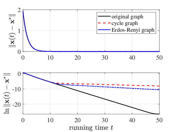
In order to make some comparisons, we also use directed cycle graph and undirected Erdos-Renyi (ER) graph for the algorithm. The performance of the algorithm with these graphs is shown in Fig. 4.

These results indicate that our distributed algorithm exponentially converges to the Nash equilibrium.

Finally, we use the undirected ER graph to compare our algorithm with the one given in Liang2017Distributed. The numerical results are shown in Fig. 5. It indicates that our algorithm converges faster than that algorithm. In addition, only our algorithm applies to directed graphs such as the original graph and the directed cycle graph.

A distributed algorithm has been proposed for Nash equilibrium seeking of aggregative games, where the strategy set can be constrained and the network is described by a weight-balanced graph. The exponential convergence has been established. The effectiveness of our method has also been illustrated by a numerical example. Further work may consider generalized Nash equilibrium seeking problem for aggregative games with coupled constraints.

The authors confirm that there are no known conflicts of interest associated with this publication and there has been no significant financial support for this work that could have influenced its outcome.

We confirm that the manuscript has been read and approved by all named authors and that there are no other persons who satisfied the criteria for authorship but are not listed. We further confirm that the order of authors listed in the manuscript has been approved by all of us.

This paper was supported in part by National Natural Science Foundation of China under Grant 61903027,72171171,62003239, and in part by Shanghai Municipal Science and Technology Major Project under grant 2021SHZDZX0100, and in part by Shanghai Sailing Program under Grant Nos. 20YF1453000.

References

• (1) Gharesifard, B., Başar, T., Dominguez-Garcia, A.D.: Price-based coordinated aggregation of networked distributed energy resources. IEEE Transactions on Automatic Control 61(10), 2936–2946 (2016)
• (2) Ye, M., Hu, G.: Distributed Nash equilibrium seeking in multiagent games under switching communication topologies. IEEE Transactions on Cybernetics 48(11), 3208–3217 (2018)
• (3) Salehisadaghiani, F., Shi, W., Pavel, L.: Distributed Nash equilibrium seeking under partial-decision information via the alternating direction method of multipliers. Automatica 103, 27–35 (2019)
• (4) Yi, P., Pavel, L.: An operator splitting approach for distributed generalized Nash equilibria computation. Automatica 102, 111–121 (2019)
• (5) Zeng, X., Chen, J., Liang, S., Hong, Y.: Generalized Nash equilibrium seeking strategy for distributed nonsmooth multi-cluster game. Automatica 103, 20–26 (2019)
• (6) Lei, J., Shanbhag, U.V.: Asynchronous schemes for stochastic and misspecified potential games and nonconvex optimization. Operations Research 68(6), 1742–1766 (2020)
• (7) Osborne, M.J., Rubinstein, A.: A Course in Game Theory. MIT Press, Cambridge, MA (1994)
• (8) Barrera, J., Garcia, A.: Dynamic incentives for congestion control. IEEE Transactions on Automatic Control 60(2), 299–310 (2015)
• (9) Cornes, R.: Aggregative environmental games. Environmental & Resource Economics 63(2), 339–365 (2016)
• (10) Ye, M., Hu, G.: Game design and analysis for price-based demand response: an aggregate game approach. IEEE Transactions on Cybernetics 47(3), 720–730 (2017)
• (11) Nocke, V., Schutz, N.: Multiproduct-firm oligopoly: an aggregative games approach. Econometrica 86(2), 523–557 (2018)
• (12) Koshal, J., Nedić, A., Shanbhag, U.V.: Distributed algorithms for aggregative games on graphs. Operations Research 63(3), 680–704 (2016)
• (13) Liang, S., Yi, P., Hong, Y.: Distributed Nash equilibrium seeking for aggregative games with coupled constraints. Automatica 85(11), 179–185 (2017)
• (14) Deng, Z., Nian, X.: Distributed generalized Nash equilibrium seeking algorithm design for aggregative games over weight-balanced digraphs. IEEE Transactions on Neural Networks and Learning Systems 30(3), 695–706 (2019)
• (15) Zhang, Y., Liang, S., Wang, X., Ji, H.: Distributed Nash equilibrium seeking for aggregative games with nonlinear dynamics under external disturbances. IEEE Transactions on Cybernetics 50(12), 4876–4885 (2019)
• (16) Parise, F., Gentile, B., Lygeros, J.: A distributed algorithm for almost-Nash equilibria of average aggregative games with coupling constraints. IEEE Transactions on Control of Network Systems 7(2), 770–782 (2020)
• (17) Yi, P., Hong, Y., Liu, F.: Initialization-free distributed algorithms for optimal resource allocation with feasibility constraints and its application to economic dispatch of power systems. Automatica 74(12), 259–269 (2016)
• (18) Facchinei, F., Pang, J.: Finite-Dimensional Variational Inequalities and Complementarity Problems. Operations Research. Springer, New York (2003)
• (19) Godsil, C., Royle, G.F.: Algebraic Graph Theory. Graduate Texts in Mathematics, vol. 207. Springer, New York (2001)
• (20) Horn, R.A., Johnson, C.R.: Matrix Analysis, 2nd edn. Cambridge University Press, Cambridge (2013)
• (21) Nedić, A., Olshevsky, A., Shi, W.: Achieving geometric convergence for distributed optimization over time-varying graphs. SIAM Journal on Optimization 27(4), 2597–2633 (2017)
• (22) Liang, S., Wang, L., Yin, G.: Exponential convergence of distributed primal-dual convex optimization algorithm without strong convexity. Automatica 105, 298–306 (2019)