The Canonical Distortion Measure for Vector Quantization and Function ApproximationThanks: This work was supported in part by EPSRC grant #K70366 and #K70373

Other authors have investigated the possibility for using specially tailored distance functions in both machine learning and vector quantization contexts. The authors of [11] used a measure of distance that takes into account invariance with respect to affine transformations and thickness transformations of handwritten characters. They achieved a notable improvement in performance using this measure in a nearest neighbour classifier. Independently but simultaneously with some of the work in a previous incarnation of this paper [1], the authors of [12] proposed an “invariance measure” on images that has a close relationship to the CDM defined here, under certain restrictions on the functions in the environment. They also presented techniques for using the invariance measure to facilitate the learning of novel tasks. In work that is close to the spirit of the present paper, the authors of [9] considered vector quantization in a Bayes classifier environment. They modified the usual squared Euclidean reconstruction error ((2) in section 2.1 below, with $d=\|\cdot\|^{2}$) by adding a Bayes risk term, and presented results showing improved combined quantization and classification performance in several real-world problems. The relationship between all these approaches and the CDM is discussed further in section 5.

As an historical note, the idea of using a set of functions to generate a pseudo-metric was used at least twenty years ago as a technical tool in the theory of topology [4], although that application has little to do with the present paper.

As any real digital communication channel has only finite capacity, transmitting continuous data (e.g speech signals or images) requires first that such data be transformed into a discrete representation. Typically, given a probability space $(X,\Sigma,P)$ ($\Sigma$ is a $\sigma$-algebra of subsets of $X$ and $P$ is the probability distribution on $X$), one chooses a quantization or codebook $\{x_{1},\dots,x_{k}\}\subset X$, and instead of transmitting $x\in X$, the index of the “nearest” quantization point

is transmitted, where $d$ is a distortion measure (not necessarily a metric) on $X$. The quantization points ${\vec{x}}=\{x_{1},\dots,x_{k}\}$ are chosen so that the expected distortion between $x$ and its quantization $q_{d}(x)$ is minimal, i.e ${\vec{x}}$ are chosen to minimize the reconstruction error

A common approach to minimizing (2) is Lloyd’s algorithm which iteratively improves a set of quantization points based on a centroidal update (see [8, 5, 7]).

Some examples of distortion measures are the Hamming metric,

where $\delta$ is the Kronecker delta function, and the squared Euclidean distortion measure for vector-valued $X$,

The use of these distortion measures has more to do with their convenient mathematical properties than their applicability to any particular problem domain. For example, suppose $X$ is a space of images and it is images of characters that are being transmitted over the channel. An image of the character “A” and another translated image of the same character would be considered “close” in this context, although the squared Euclidean distance between the two images would be large, quite likely larger than the distance between an image of “A” and an image of “B” in the same location. Thus the squared Euclidean distortion measure does not capture well the idea of two images being “close”. Another example is that of speech coding—there is a large squared Euclidean distance between a speech signal and a small translation of it in time, although both sound very similar to a human observer. A vector quantizer constructed using an inappropriate distortion measure will require a far larger set of quantization points to achieve satisfactory performance in environments where we are primarily interested in the subjective quality of the reconstruction. And in almost all applications of vector quantization it is the subjective quality of the reconstruction that is the most important: eventually the quality of the reconstructed speech signal or image is measured by how close it appears to be to the original for some observer.

In the next section we will see how the problem of choosing an appropriate distortion measure may be solved, at least in principle, by using the idea of the environment of a quantization process.

What makes the translated image of an “A” close to the original, while an untranslated image of a “B” quite distant? And what makes two speech signals nearly identical even though they are miles apart from a Euclidean perspective? As discussed in the introduction, it is because there is an environment of functions (the character classifiers) that vary little across images of the same character, and similarly there is an environment of “speech classifiers” that vary little across utterances of the same sentences or words.

Note that the set of possible character classifiers is much larger than the set of particular classifiers for the English alphabet (English language). The particular form of the letters we use is arbitrary (as evidenced by the existence of vastly different alphabets such as Hebrew or Kanji), the only thing that is required of a character is that different examples of it are recognisably the same object (to us). Thus the number of different character classifiers is potentially astronomical. A similar conclusion holds for speech: the set of spoken word classifiers is nearly infinite if one includes all possible words from all possible languages.

To formalize the idea that it is an environment of functions that determines the distortion measure on the input space, define the environment of any probability space $(X,\Sigma,P)$ to be a pair $({\cal F},Q)$ where ${\cal F}$ is a set of functions mapping $X$ into a space $(Y,\sigma)$, where $\sigma\colon Y\times Y\to{R}$ ($\sigma$ may be a metric), and $Q$ is a probability measure on ${\cal F}$¹¹ 1 For $Q$ to be well defined there needs to be a $\sigma$-algebra on ${\cal F}$. We leave that algebra unspecified in what follows, and simply assume that an appropriate one exists.. An environment so defined induces the following natural distortion measure on $X$:

for all $x,x^{\prime}\in X$. In words, $\rho(x,x^{\prime})$ is the average distance between $f(x)$ and $f(x^{\prime})$ where $f$ is a function chosen at random from the environment.

Note that if $\sigma$ is a metric on $Y$ then $\rho$ is a pseudo-metric on $X$ (recall that a pseudo-metric is the same as a metric except that $\rho(x,x^{\prime})=0$ does not necessarily imply $x=x^{\prime}$). From now on $\rho$ will be referred to as the Canonical Distortion Measure or CDM for the environment $({\cal F},Q)$.

In relation to the character transmission problem, ${\cal F}$ would consist of all character like classifiers, $Y$ would be the set $[0,1]$ and we could take $\sigma(y,y^{\prime})=(y-y^{\prime})^{2}$ (here we are assuming that the functions $f\in{\cal F}$ are probabilistic classifiers, that is $f(x)$ represents the probability that $x$ belongs to the category represented by $f$). Given our limited capacity to learn characters, we could take the environmental probability measure $Q$ to have support on at most 10,000 distinct elements of ${\cal F}$ (so ${\cal F}$ must contain more than just the 26 English letters). Then if $x$ and $x^{\prime}$ are two images of the same character, $f(x)\approx f(x^{\prime})$ for all $f$ in the support of $Q$ and so by (3), $\rho(x,x^{\prime})\approx 0$, as required. If $x$ and $x^{\prime}$ are images of different characters, the classifiers $f_{x}$ and $f_{x^{\prime}}$ corresponding to $x$ and $x^{\prime}$ would have $f_{x}(x)\approx 1,f_{x}(x^{\prime})\approx 0$ and $f_{x^{\prime}}(x)\approx 0,f_{x^{\prime}}(x^{\prime})\approx 1$. Classifiers for characters that are subjectively similar to $x$ ($x^{\prime}$) will behave in a similar way to $f_{x}$ ($f_{x^{\prime}}$), except that they will not assign such a high value to positive examples as $f_{x}$ and $f_{x^{\prime}}$ do. All other classifiers $f$ will have $f(x)\approx f(x^{\prime})\approx 0$. Substituting this into (3) shows $\rho(x,x^{\prime})$ will be larger if $x$ and $x^{\prime}$ are images of different characters than if they are images of the same characters.

Note that $\rho$ depends only upon the environment $({\cal F},Q)$ and not upon $X$ or its probability measure $P$. Thus problems with the same $X$ but different environments (for example character classification and face recognition—different environments for the space of images) will generate different canonical distortion measures. In the next section we will show that $\rho$ is the optimal distortion measure to use if piecewise constant approximation of the functions in the environment is the aim. Thus the fact that different environments generate different $\rho$’s shows that the optimal similarity measure between data points is highly dependent on what one is planning to do with the data.

The definition of $\rho$ does not restrict us to considering only classifier environments, any kind of functions will do. For example, the environment might consist of all bounded linear functions on some compact subset of $X={R}^{n}$, all threshold functions or all polynomials up to a certain degree. Noisy environments can also be modelled within this framework by making the functions $f\in{\cal F}$ distribution valued. For example, if the problem is to learn noisy concepts then these can be represented as a distribution $P$ on $X$ combined with a conditional distribution on $\{0,1\}$. Different concepts would have different conditional distributions, which we can represent as mappings $f\colon X\to Y$ where now $Y$ is the set of all distributions on $\{0,1\}$. The distance measure $\sigma$ is now a distance measure on probability distributions, such as Kullback-Liebler divergence or Hellinger distance. The CDM between two inputs $x$ and $x^{\prime}$ would then equal the average distance between the distributions $f(x)$ and $f(x^{\prime})$.

Suppose that $X={R}^{n}$ and ${\cal F}$ consists of all linear maps from $X$ into ${R}$. ${\cal F}$ is the vector space dual of $X$ and so is itself isomorphic to ${R}^{n}$. With this in mind, take the measure $Q$ on ${\cal F}$ to be Lebesgue measure on ${R}^{n}$, but restrict $Q$’s support to the cube $[-\alpha,\alpha]^{n}$ for some $\alpha>0$, and renormalise so that $Q([-\alpha,\alpha]^{n})=1$. Let $\sigma(y,y^{\prime})=(y-y^{\prime})^{2}$ for all $y,y^{\prime}\in{R}$. $\rho$ can then be reduced as follows:

Thus a linear environment induces the squared Euclidean distance on $X$. The reverse conclusion is also true, i.e. if one assumes that $\rho(x,x^{\prime})=K\|x-x^{\prime}\|^{2}$ for all $x,x^{\prime}$ then ${\cal F}$ must be a linear function class (almost everywhere). So based on the optimality result of the next section, using the squared Euclidean distortion is optimal if one wishes to approximate linear functions on the input space, but is not optimal for any other environments. As it is very rare that one is interested in applying linear functions to images, or speech signals (for example face classifiers are not linear maps on image space, nor are word classifiers linear maps on speech signals), the use of squared Euclidean distortion in these environments is not the best thing to do.

Note that a uniform distribution over any symmetric region of weight space will yield a CDM that is proportional to Euclidean distance, while a general distribution will yield a CDM that is a quadratic form $\rho(x,x^{\prime})=\langle x|A|x^{\prime}\rangle$ where $A$ is an $n\times n$ matrix.

Take the same example as above but this time threshold the output of each $f\in{\cal F}$ with the Heaviside step function, and take $Q$ to have support only on the unit ball in ${R}^{n}$, rather than the cube, $[-\alpha,\alpha]^{n}$ (this is done to make the calculations simple). After some algebra we find

where $\theta$ is the angle between $x$ and $x^{\prime}$. Thus in an environment consisting of linear classifiers (i.e. thresholded linear functions) whose coefficients are distributed uniformly in the unit ball, the natural distortion measure on the input space is the angle between two input vectors.

Let $X=Y=[-1,1]$, $\sigma(y,y^{\prime})=|y-y^{\prime}|$ for all $y,y^{\prime}\in Y$ and let ${\cal F}=\{f\colon x\mapsto ax^{2}\}$ with $a$ uniformly distributed in the range $[-1,1]$. With this environment,

Note that $\rho(x,y)=0$ if $x=y$ and if $x=-y$, so that $x$ and $-x$ are zero distance apart under $\rho$. This reflects the fact that $f(x)=f(-x)$ for all $f\in{\cal F}$. Notice also that $\rho(x,y)$ is the ordinary Euclidean distance between $x$ and $y$, scaled by $|x+y|$. Thus two points with fixed Euclidean distance become further and further apart under $\rho$ as they are moved away from the origin. This reflects the fact that the quadratic functions in ${\cal F}$ have larger variation in their range around large values of $x$ than they do around small values of $x$. This can also be seen by calculating the ${\varepsilon}$-ball around a point $x$ under $\rho$ (i.e the set of points $x^{\prime}\in X$ such that $\rho(x,x^{\prime})\leq{\varepsilon}$). To first order in ${\varepsilon}/{x}$ this is

Note that the Euclidean diameter of the ${\varepsilon}$-ball around $x$ decreases inversely linearly with $x$’s—Euclidean again—distance from the origin.

For the quadratic environment of example 3.3, the optimal quantization for $k=6$ is shown in figure 2 along with $f$ and ${\hat{f}}_{\rho}$ for $f(x)=x^{2}$. Note how the optimal quantization reduces the deviation between $f$ and its approximation ${\hat{f}}_{\rho}$ by spacing the points closer together for larger values of $x$.

To calculate the optimal quantization in this case, first note that by the symmetry of the environment, the quantization points $\{x_{1},\dots,x_{6}\}$ can all be assumed to be positive, and without loss of generality suppose that $x_{1}\leq x_{2}\leq\dots\leq x_{6}$. Direct calculation of the reconstruction error $E_{\rho}({\vec{x}})$ (2) shows that

A similar procedure can be used to show that $x_{1}$ and $x_{6}$ must satisfy,

Optimal quantization points can be found by solving these equations numerically.

The authors of [11] introduced a technique for comparing handwritten characters called Transformation Distance. They observed that images of characters are invariant under transformations such as rotation, dilation, shift, line thickening and so on. Denoting the set of all such transformations by $G$, and assuming that $G$ can be parameterised by $k$ real parameters, they noted that for each character $x$, the set

forms a $k$-dimensional manifold in the input space $X$. They defined the distance bewteen two images $x$ and $x^{\prime}$ to be:

that is, $D(x,x^{\prime})$ is the smallest Euclidean distance between any transformed image of $x$ and $x^{\prime}$ (and is called the transformation distance between $x$ and $x^{\prime}$). In order to simplify the computation, in [11] $D(x,x^{\prime})$ was approximated by a linearised version. However we will concentrate on the exact expression (7).

Relating the transformation distance to the CDM, note that invariance of characters under the action of $G$ is equivalent to assuming that all character classifiers in the environment ${\cal F}$ are invariant under the action of $G$. In other words, for all $f\in{\cal F}$, $f(gx)=f(x)$ for all $g\in G$. Then clearly, if $x^{\prime}\in{\cal M}(x)$, $\rho(x,x^{\prime})=D(x,x^{\prime})=0$, so the CDM gives the same answer as the transformation distance in this case. However, if $x^{\prime}\notin{\cal M}(x)$ then it is unlikely that $D(x,x^{\prime})$ and $\rho(x,x^{\prime})$ will be the same, because $D(x,x^{\prime})$ (somewhat arbitrarily) measures the Euclidean distance between the manifolds ${\cal M}(x)$ and ${\cal M}(x^{\prime})$, whereas $\rho(x,x^{\prime})$ performs an average over the functions in the environment to compute the distance.

The transformation distance and the CDM share the important property that the distance between any pair of points in ${\cal M}(x)$ and ${\cal M}(x^{\prime})$ respectively is always the same. This is trivial by the construction of $D$; to see it for the CDM let $x,x^{\prime}\in{\cal M}(x)$ and $y,y^{\prime}\in M(y)$. Then $\rho(x,x^{\prime})=\rho(y,y^{\prime})=0$ and combining this with the triangle inequality gives:

Running the same argument with $x$ and $x^{\prime}$ and $y$ and $y^{\prime}$ interchanged shows that $\rho(x,y)=\rho(x^{\prime},y^{\prime})$ always.

In [6], Edelman introduced a concept of representation he called the Chorus of Prototypes. The idea is to train a set of real-valued classifiers, $f_{1},\dots,f_{N}$, for a domain of prototype objects (so that $f_{i}(x)\in[0,1]$ is interpreted as the probability that $x$ is an example of object $i$). All objects (not just the prototypes) are then represented by the vector of activations they induce at the output of the prototype classifiers. This vector of activations is a Low Dimensional Representation (LDR) of the input space. It is argued that the Euclidean distance between two representation vectors corresponds to the distal similarity of the objects.

Given that both the CDM and the Chorus of Prototypes represent similarity by making use of an environment of classifiers, it is natural to look for a connection between the two. There is a connection if one assumes that all functions in the environment can be implemented as linear maps composed with a fixed low dimensional representation. So let $h=(h_{1},\dots,h_{k})\colon{R}^{d}\to{R}^{k}$ ($d\gg k$) be the fixed LDR, and then each $f\in{\cal F}$ is of the form $\sum w_{i}h_{i}$ where the $w_{i}$ depend on $f$. Suppose that $k$ is minimal. Note that the $f$ take values outside the range $[0,1]$ and so cannot be interpreted as probabilities. However we can still interpret the output of $f$ as a “degree of classification”—large positive values being high confidence and large negative values low confidence. In this case the environmental distribution $Q$ is a distribution over the weights $w$. If $Q$ is uniform over a symmetric region of weight space then by section 3.1, the CDM between two inputs $x$ and $x^{\prime}$ will be proportional to the Euclidean distance between their transformed representations $h(x)$ and $h(x^{\prime})$.

Now choose any $f_{1},\dots,f_{k}$ such that their respective weight vectors $w^{1},\dots,w^{k}$ are linearly independent (such a set of functions can always be found because we assumed $k$ is minimal). $(f_{1},\dots,f_{k})$ will be the chorus of prototypes representation. Set

and note that $W$ is nonsingular. For any input $x$, $(f_{1}(x),\dots,f_{k}(x))$ (the representation of $x$ by its similarity to the prototypes $i=1,\dots,k$) is equal to $Wh(x)$. Let $f=w\cdot h$ be any classifier in the environment. Set $w^{\prime}:=wW^{-1}$. Then $f=w^{\prime}Wh=\sum w^{\prime}_{i}f_{i}(x)$. Thus any classifier in the environment is representable as a linear combination of prototype classifiers, as required for the chorus of prototypes idea.

The authors of [12] defined an “invariance function” $\sigma\colon X\times X\to\{0,1\}$ for a finite environment ${\cal F}$ with the property that if there exists $f\in{\cal F}$ such that $f(x)=1$ then $f^{\prime}(x)=0$ for all other $f^{\prime}\in{\cal F}$:

If we assume the environmental distribution $Q$ is uniform on ${\cal F}$, a quick calculation shows that for all $x,x^{\prime}$ for which $\sigma(x,x^{\prime})$ is defined,

Thrun and Mitchell also showed how $\sigma$ can be used to facilitate learning of novel tasks within their lifelong learning framework.

To generate training sets for learning the CDM, both the distribution $Q$ over the environment ${\cal F}$ and the distribution $P$ over the input space $X$ must be sampled. So let $\{f_{1},\dots,f_{M}\}$ be $M$ i.i.d. samples from ${\cal F}$ according to $Q$ and let $\{x_{1},\dots,x_{N}\}$ be $N$ i.i.d. samples from $X$ according to $P$. For any pair $x_{i},x_{j}$ an estimate of $\rho(x_{i},x_{j})$ is given by

This generates $N^{2}$ training triples,

which can be used as data to train a neural network. That is, the neural network would have two sets of inputs—one set for $x_{i}$ and one set for $x_{j}$—and a real-valued output $\rho^{*}(x_{i},x_{j})$ representing the network’s estimate of ${\hat{\rho}}(x_{i},x_{j})$. The mean-squared error of the network on the training set is then

$E$ is an estimate of the true distance between the network’s $\rho^{*}$, and the true CDM $\rho$, where this is defined by:

Note that the process of sampling from ${\cal F}$ to generate $f_{1},\dots,f_{M}$ is a form of multi-task learning (see e.g. [2, 3, 12, 10]) and that such sampling is a necessary condition for the empirical estimate of the CDM, $\rho^{*}$, to converge to the true CDM $\rho$.

An artificial environment was created to test the effectiveness of training neural networks to learn the CDM. The environment was chosen to consist of a set of two link “robot arm” problems. That is, each function in the environment corresponded to a robot arm with two links of length $r_{1}$ and $r_{2}$ (see Figure 4. Note that the term “robot” is used fairly loosely here: the example doesn’t have much to do with robotics). The function corresponding to $r_{1},r_{2}$ is the map $f_{r_{1},r_{2}}\colon[-\pi,\pi]^{2}\to[0,(r_{1}+r_{2})^{2}]$ that computes the square of the distance of the end of the arm from the origin, given the angles of the links $\theta_{1},\theta_{2}$. Thus, $f_{r_{1},r_{2}}(\theta_{1},\theta_{2})=r_{1}^{2}+r_{2}^{2}+2r_{1}r_{2}\cos(\theta_{1}-\theta_{2})$. The link lengths $r_{1}$ and $r_{2}$ were chosen uniformly in the range $[0,1]$, so that ${\cal F}=\{f_{r_{1},r_{2}}\colon(r_{1},r_{2})\in[0,1]^{2}\}$. The goal was to train a neural network to correctly implement the CDM $\rho((\theta_{1},\theta_{2}),(\theta^{\prime}_{1},\theta^{\prime}_{2}))$. Note that in this case $\rho$ can be calculated in closed form:

The network architecture used was a single hidden layer neural network with $\tanh$ activation function on the hidden layer nodes and a linear output node. After some experimentation twenty hidden nodes was found to be sufficient. The network had four inputs, one each for $\theta_{1},\theta_{2},\theta^{\prime}_{1}$ and $\theta^{\prime}_{2}$. The knowledge that $\rho$ is symmetric was built into the network by taking the output of the network for inputs $x_{i}$ and $x_{j}$ to be

rather than just the “raw” network output $\rho^{*}(x_{i},x_{j})$. Note that (13) is automatically symmetric in $x_{i}$ and $x_{j}$. With this choice of the estimate of $\rho$, the error measure (10) becomes

Back-propagation was used to compute the gradient of (14).

Training sets were generated by first sampling $M$ times from the environment to generate $f_{1},\dots,f_{M}$, which in this case meant generating M pairs $(r_{1},r_{2})$ uniformly at random in the square $[0,1]^{2}$. Then the input space $[-\pi,\pi]^{2}$ was sampled uniformly at random $N$ times to generate $x_{1},\dots,x_{N}$ and the empirical estimate ${\hat{\rho}}(x_{i},x_{j})$ was constructed using (9) for each of the $N(N+1)/2$ pairs $(x_{i},x_{j})$ for $1\leq i\leq j\leq N$. A separate cross-validation set was also generated using the same values of $M$ and $N$ used for the training set. The network was trained using conjugate gradient descent—with the gradient computed from (14)—until the error on the cross-validation set failed to decrease for more than five iterations in a row. After the network had been trained, an initial quantization set ${q_{1},\dots,q_{m}}$ of size $m\ll N$ was chosen uniformly at random from $\{x_{1},\dots,x_{N}\}$ and then the empirical Lloyd algorithm [8] was used to optimize the positions of the quantization points. The trained neural network—suitably symmetrised via (13)—was used as the distortion measure.

Several different experiments were performed with different values of $M,N$ and $m$—the Voronoi regions for $(M,N,m)=(100,100,20)$ are plotted in Figure 6, along with the optimal quantization set and corresponding Voronoi regions for the true CDM (12). Note that the regions generated by the neural net approximation are very similar to those generated by the true CDM. The reconstruction error of the input space was estimated from the training set $\{x_{1},\dots,x_{N}\}$ and also calculated (nearly) exactly by quantizing the input space into a $250\times 250$ grid. These quantities are shown in the first two columns of table 1 for several different values of $M,N$ and $m$. Note the good agreement between the estimate ${\hat{E}}_{\rho^{*}}$ and the “true” value $E_{\rho^{*}}$ in each case, and also that the reconstruction error is very small in all cases, improving as the training set size ($M,N$) for the CDM increases, and also as the number of quantization points $m$ increases.

Recall that by lemma 1, $E_{\rho^{*}}(q_{1},\dots,q_{m})$ equals the reconstruction error of the functions in the environment ($E^{\rho^{*}}_{\cal F}(q_{1},\dots,q_{m})$). That is, if

1. 1.

   a function $f$ is picked at random (i.e. the link lengths $r_{1}$ and $r_{2}$ are picked at random),

2. 2.

   the values $f(q_{i})$ for each $q_{i}$ in the optimal quantization set are generated and stored, and

3. 3.

   the value of $f$ at any novel input $x\in X$, chosen according to $P$, is estimated by $f(q_{\rho^{*}}(x))$,

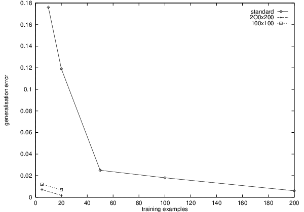
then $E_{\rho^{*}}(q_{1},\dots,q_{m})$ is the expected generalisation error: $E_{X}\left[f(x)-f(q_{\rho^{*}}(x))\right]^{2}$. Hence a small value of $E_{\rho^{*}}(q_{1},\dots,q_{m})$ indicates that any function in the environment is likely to be learnable to high accuracy by this procedure²² 2 Note that this procedure is just $1$ Nearest Neighbour, with $\rho^{*}$ as the distance metric and the quantization points intelligently placed.. To demonstrate this, $E^{\rho^{*}}_{\cal F}(q_{1},\dots,q_{m})$ was estimated by generating 100 new functions at random from the environment and learning them according to the above procedure. Each function’s generalisation error was estimated using a fine grid on the input space, and then averaged across all $100$ functions. The average generalisation error is plotted in the third column of table 1 for the various CDMs generated from different training set sizes and the different numbers of quantization points. Note the good agreement between the reconstruction error of the environment (${\hat{E}}^{\rho^{*}}_{\cal F}$) and the reconstruction error of the input space $E_{\rho^{*}}$.

For comparison purposes the same 100 functions were learnt using a 10-hidden node neural network, without the assistance of the CDM. The average generalisation error across all $100$ functions is displayed in Figure 8 along with the same quantity for the piecewise-constant approximations. The piecewise-constant approach based on the estimated CDM is clearly superior to the normal approach approach in this case.

References

- [1] Jonathan Baxter. Learning Internal Representations. PhD thesis, Department of Mathematics and Statistics, The Flinders University of South Australia, 1995. Draft copy in Neuroprose Archive under “/pub/neuroprose/Thesis/baxter.thesis.ps.Z”.
- [2] Jonathan Baxter. Learning Internal Representations. In Proceedings of the Eighth International Conference on Computational Learning Theory, Santa Cruz, California, 1995. ACM Press.
- [3] Richard Caruana. Learning Many Related Tasks at the Same Time with Backpropagation. In Advances in Neural Information Processing 5, 1993.
- [4] W W Comfort and S Negropontis. Continuous Pseudometrics. M Dekker, New York, 1975.
- [5] T M Cover and J A Thomas. Elements of Information Theory. John Wiley & Sons, Inc., New York, 1991.
- [6] Shimon Edelman. Representation, similarity, and the chorus of prototypes. Minds and Machines, 5:–, 1995.
- [7] A Gersho and R M Gray. Vector Quantization and Signal Processing. Kluwer Academic Publishers, 1992.
- [8] S P Lloyd. Least squares quantization in pcm. Technical report, Bell Laboratories, 1975.
- [9] Karen L Oehler and Robert M Gray. Combining image compression and classification using vector quantozation. IEEE Transactions on Pattern Analysis and Machine Intelligence, 17(5):461–473, May 1995.
- [10] Lori Y Pratt. Discriminability-based transfer between neural networks. In Stephen J Hanson, Jack D Cowan, and C Lee Giles, editors, Advances in Neural Information Processing Systems 5, pages 204–211, San Mateo, 1992. Morgan Kaufmann.
- [11] Patrice Simard, Yann LeCun, and John Denker. Efficient pattern recognition using a new transformation distance. In S J Hanson, J D Cowan, and C Lee Giles, editors, Advances in Neural Information Processing Systems 5, pages 51–58, San Mateo, 1993. Morgan Kauffman.
- [12] Sebastian Thrun and Tom M Mitchell. Learning One More Thing. Technical Report CMU-CS-94-184, CMU, 1994.
Received Date
Accepted Date
Final Manuscript Date