rFIA: An R package for estimation of forest attributes with the US Forest Inventory and Analysis DatabaseJournal: Environmental Modelling and Software
Abstract
Forest Inventory and Analysis (FIA) is a US Department of Agriculture Forest Service program that aims to monitor changes in forests across the US. FIA hosts one of the largest ecological datasets in the world, though its complexity limits access for many potential users. rFIA is an R package designed to simplify the estimation of forest attributes using data collected by the FIA Program. Specifically, rFIA improves access to the spatio-temporal estimation capacity of the FIA Database via space-time indexed summaries of forest variables within user-defined population boundaries (e.g., geographic, temporal, biophysical). The package implements multiple design-based estimators, and has been validated against official estimates and sampling errors produced by the FIA Program. We demonstrate the utility of rFIA by assessing changes in abundance and mortality rates of ash (Fraxinus spp.) populations in the Lower Peninsula of Michigan following the establishment of emerald ash borer (Agrilus planipennis).
Keywords:
Forest Inventory and Analysis, R package, rFIA1 Introduction
Forest Inventory and Analysis (FIA) is a United States Department of Agriculture Forest Service program with the goal of monitoring and projecting changes in forests across the United States (US) [USDA Forest Service 2019b]. The program collects, publishes, and analyzes data describing the extent, condition, volume, growth, and use of trees from all land ownerships in the nation, with some records dating back to the early 1930s [Tinkham et al. 2018, Smith 2002]. In 1999, the FIA program established a systematic grid of permanent ground plots that are evenly divided into panels measured in a continuous cycle, allowing spatially unbiased estimates of forest attributes to be computed on an annual basis [Gillespie 1999, Smith 2002]. The flexibility inherent to the FIA inventory system creates unprecedented opportunities to assess forest change across space, through time, and within unique populations of interest [Tinkham et al. 2018, Gray et al. 2012].
The research significance of the FIA program has increased in recent decades, with primary applications in carbon cycling, forest growth, forest health, and remote sensing [Tinkham et al. 2018]. The FIA program hosts one of the largest ecological datasets in the world by spatial and temporal extent [Tinkham et al. 2018], including records from over 5.8 million trees measured at least twice and encompassing a range of ecological diversity unmatched by any other large-scale national forest inventory system [Tomppo et al. 2010]. The breadth of attributes currently measured by the FIA program, ranging from forest composition and structure to soil chemistry and invasive species abundance, makes it a vast and powerful resource for monitoring the status and trends in forest attributes from the scale of individual trees to subcontinents [Tinkham et al. 2018].
The primary limitation for individuals using FIA data in their own analyses is the complex sample design, database structure, and Structured Query Language used by the FIA program [Tinkham et al. 2018, Kromroy et al. 2008]. FIA data are publicly available in several formats (e.g., FIA DataMart) and estimation is facilitated through online tools (e.g., EVALIDator) [USDA Forest Service 2019a, Pugh et al. 2018] and a non-public R package, FIESTA [Frescino et al. 2015]. That said, FIA data are difficult for many non-FIA users to interpret and understand [Tinkham et al. 2018] and there is potential to increase the use of these incredibly rich data among industry professionals, academic scientists, and the general public. To promote use of this valuable public resource and extend the reach of the FIA program and the publicly available data, there is a need for a flexible, user-friendly tool that simplifies the process of working with FIA data for experts and novices alike. To this end, we developed rFIA, an add-on package for R [R Core Team 2018a].
rFIA implements FIA’s design-based estimation procedures [Bechtold et al. 2005] for over 50 forest attributes using a simple, yet powerful design. rFIA greatly improves access to the spatio-temporal estimation capacity inherent to the FIA program by allowing space-time indexed summaries of forest attributes to be produced within user-defined population boundaries (e.g., geographic, temporal, biophysical). The package enhances the value of FIA for temporal change detection and forest health monitoring by implementing five design-based estimators that offer flexibility in a balance between precision and temporal smoothing. Our intention in developing rFIA is to provide a versatile, user-friendly software that allows all R users to unlock the value of the FIA program.
2 Methods
2.1 Software design
We designed rFIA to be intuitive to use and support common data representations by directly integrating other popular R packages into our development. We achieve efficient joins, queries, and data summaries with the dplyr package [Wickham et al. 2015]. Specifically, we leverage dplyr for joining and filtering FIA tables, facilitating hierarchical grouping of summary attributes, and implementing non-standard evaluation in rFIA core functions. We achieve efficient space-time query and summary within user-defined population boundaries (i.e., spatial polygons) with the sf package [Pebesma 2018]. Parallel processing is implemented with the parallel package [R Core Team 2018b]. Parallel implementation is achieved using a snow type cluster [Tierney et al. 2018] on any Windows OS, and with multi-core forking [R Core Team 2018b] on any Unix or Mac OS.
Software Availability Name of software rFIA Type of software Add-on package for R First available 2019 Program languages R License GPL 3 Code Repository https://cran.r-project.org/web/packages/rFIA/index.html Installation in R install.packages("rFIA") Developers Hunter Stanke, Andrew O. Finley Contact Address Department of Forestry, Michigan State University, East Lansing, MI, USA
2.2 Sampling and estimation procedures
The design-based estimation procedures used by the FIA program and implemented by rFIA have been widely described in the literature [Bechtold et al. 2005, McRoberts et al. 2005a, Hoffman et al. 2014], and hence will only be briefly described here. All estimators for population totals, ratios, and associated variances are derived from the Horvitz-Thompson estimator and hence incorporate design information via inverse-probability weighting [Horvitz & Thompson 1952]. Bechtold et al. 2005 describes in detail the theoretical basis for estimators used by the FIA program and implemented by rFIA.
The FIA program conducts forest inventories using a multi-phased sampling procedure designed to reduce variance through stratification [Bechtold et al. 2005, McRoberts et al. 2005a]. In the pre-field phase, remotely sensed imagery are used to stratify land area by determining dominant land use in each pixel within the population of interest. In the core phase, permanent ground plots are systematically distributed across the US at a rate of approximately 1 plot per 6000 acres using a hexagonal sampling frame [Bechtold et al. 2005, McRoberts et al. 2005a]. Each plot is assigned to a single stratum based on the the pre-field stratification of the plot center. If any portion of a plot is determined to contain a forest land use from pre-field stratification, a field crew will visit the site and measure core FIA variables [Bechtold et al. 2005]. In the intensive phase, additional forest and ecosystem health variables are measured on 5-15% of established core plots (approximately 1 plot per 96,000 acres).
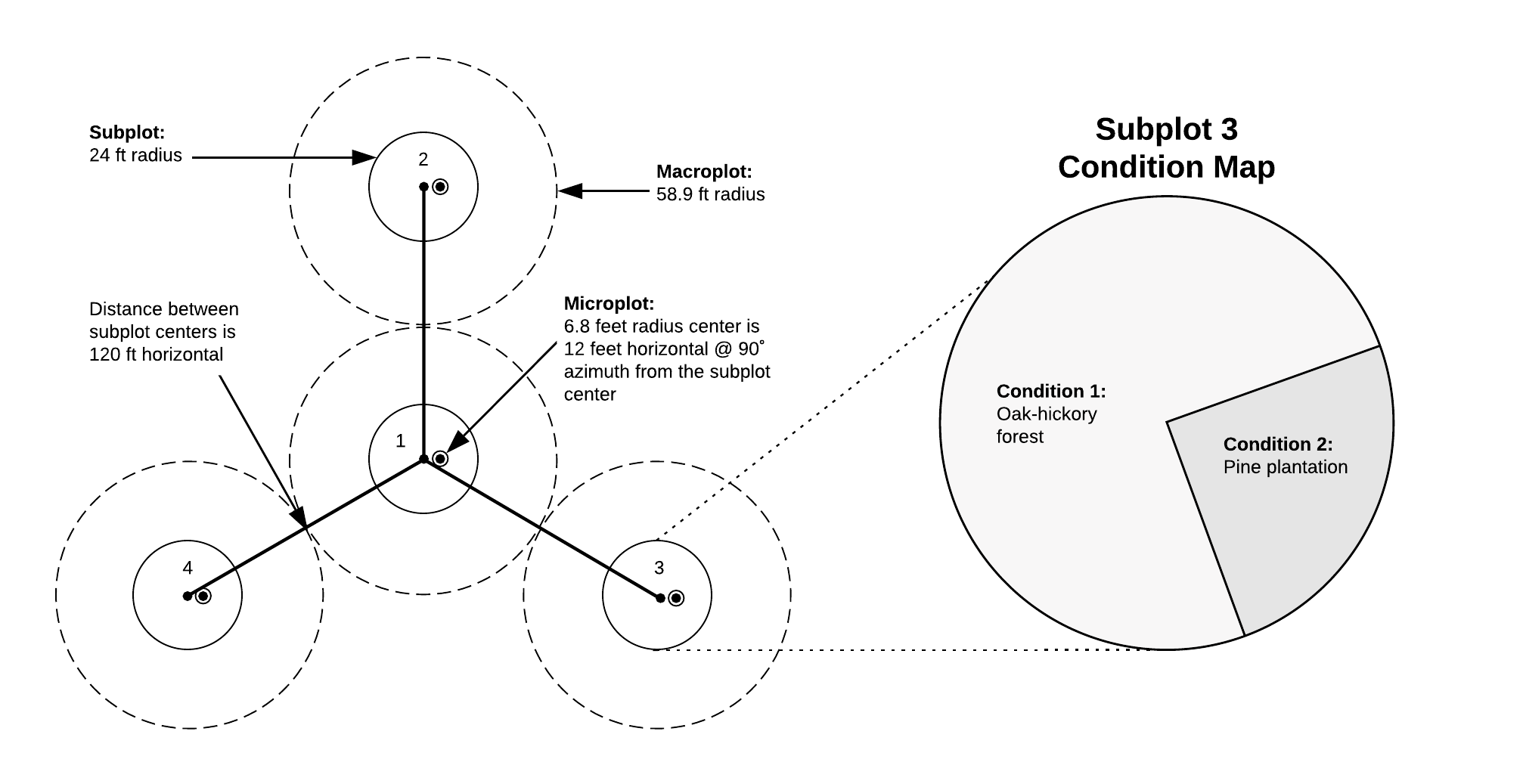
FIA permanent ground plots consist of clusters of four subplots (Figure 1), where tree attributes are measured for all stems 5.0 inches diameter at breast height (DBH) and larger. Within each subplot, a microplot is established where tree attributes are measured for saplings (1.0-4.9 inches DBH). Each subplot is surrounded by a macroplot, on which rare events such as large trees are optionally measured. In addition to tree attributes, data are collected that describe the area where trees are located on each subplot and macroplot. If area attributes (e.g., ownership group, forest type, stocking) vary substantially across a plot, the land area within the plot is divided into distinct domains referred to as condition classes so that tree data can be properly associated with area classifications (Figure 1).
Plot-level estimates of forest attributes (e.g., tree biomass, forested area) are obtained by summing observations or estimates of the attribute, which are within the population of interest (e.g., live trees, private land), across the plot. Observations are multiplied by 1 if the attribute is within the population of interest, and 0 otherwise. Thus if all observations on a plot fall outside the population of interest, observations will sum to 0 for the plot. For ratio estimates (e.g., tree biomass per unit area), it is possible to specify different populations of interest for the numerator and denominator attributes.
The FIA program uses an annual panel system to estimate both current inventory and change. Individual panels are represented by a subset of ground plots that are measured in the same year and represent complete spatial coverage across the population of interest [McRoberts & Miles 2016]. In the eastern US, inventory cycles consist of 5 or 7 annual panels, with 20 or 15 percent of ground plots measured in each year, respectively. In the western US, inventory cycles include 10 annual panels and thus 10 percent of ground plots are measured each year [Bechtold et al. 2005]. Variance reduction can often be achieved by combining current panels with data from previous panels, although FIA does not prescribe a core procedure for panel combination because a single approach is unlikely to be suitable for all estimation objectives or across a wide variety of spatial, temporal, and population conditions [Bechtold et al. 2005].
In rFIA, users may choose from one of four unique estimators that combine data from multiple panels or choose to return estimates from individual annual panels (ANNUAL), thereby forgoing panel combination entirely. The “temporally-indifferent” (TI) estimator is used by default, essentially pooling all panels within an inventory cycle into a large periodic inventory. The TI estimator is commonly used by other FIA estimation tools, like EVALIDator [USDA Forest Service 2019a, Pugh et al. 2018]. Alternatively, individual panels may be weighted by employing a moving-average estimator, including the simple moving average (SMA), linear moving average (LMA), or exponential moving average (EMA). The SMA applies equal weight to all annual panels (Eq. 1), while the LMA and EMA apply weights that decay linearly or exponentially as a function of time since measurement, respectively (Eq. 2-3). In each case of the moving average, panel weights sum to one across an inventory cycle. Panel weights are computed as follows:
| (1) | |||
| (2) | |||
| (3) |
where is the constant positive weight for annual panel, , described as the sequential index of the panel within an inventory cycle (i.e., ), is the total number of annual panels in the inventory cycle, and is a decay parameter, ranging between zero and one, that controls the behavior of the exponential weighting function (Eq. 3). As approaches 1, panel weights become nearly evenly distributed across the inventory cycle, and estimates produced by the EMA will approach those of the SMA. As approaches 0, weights are skewed towards the most recent panel and estimates of the EMA will approach those of individual annual panels. The inclusion of makes the EMA the most versatile estimator offered in rFIA.
In general, sample variance is minimized when panel weights are evenly distributed across the inventory cycle (e.g., SMA), with the trade-off of introducing temporal lag-bias by weighting recent measurements the same as older measurements. Hence, equal weighting schemes could be undesirable in settings where variable values change over time. Alternatively, applying lower weights to less recent panels reduces the effective sample size of the inventory, effectively increasing variance but reducing temporal smoothing by favoring more recent measurements. We advise users of rFIA to be aware of this trade-off between precision and temporal smoothing when considering various estimators offered in the package.
2.3 Software testing
We have conducted extensive validation for all estimated attributes for small and large areas against EVALIDator [USDA Forest Service 2019a]. Here we present an abbreviated version of a validation for the state of Connecticut in the year 2018 using the “temporally-indifferent” estimator (Table 1). Current status estimates were produced for live trees with DBH 1.0 inch and annual change estimates were produced for all stems with DBH 5.0 inches. Down woody material estimates were produced for the 1000 hour fuel class (coarse woody debris). Total forest area estimates were produced using plots containing a forested condition. All estimates and associated sampling errors produced by rFIA match those produced by EVALIDator. A detailed description of the validation described in Table 1, including code used to produce estimates using rFIA, can be found in Appendix A.
| Forest Attribute | rFIA | EVALIDator | ||
|---|---|---|---|---|
| Estimate | SE | Estimate | SE | |
| Live tree abundance () | ||||
| Live tree basal area () | ||||
| Live tree merchantable volume () | ||||
| Live tree sawlog volume () | ||||
| Live tree aboveground biomass () | ||||
| Live tree aboveground carbon () | ||||
| Annual net biomass growth ()* | ||||
| Annual mortality ()* | ||||
| Annual removals ()* | ||||
| Coarse woody material volume () | ||||
| Coarse woody material biomass () | ||||
| Coarse woody material carbon () | ||||
| Total forest area () | ||||
3 rFIA package features
rFIA is capable of estimating more forest attributes from FIA data than any other publicly available tool and offers unmatched flexibility in defining unique populations of interest and producing space-time indexed summaries of forest attributes. Users can install the released version of rFIA from CRAN (v0.1.0, 28 October 2019), or alternatively install the development version from Github (https://github.com/hunter-stanke/rFIA) using devtools [Wickham et al. 2019]. Table 2 depicts a list of core functions available in rFIA. A schematic diagram for using rFIA to produce population estimates of forest attributes can be found in Figure 2.
| Function | Description |
|---|---|
| area | Estimate land area in various classes |
| biomass | Estimate volume, biomass, and carbon stocks of standing trees |
| clipFIA | Spatial and temporal queries for FIA data |
| diversity | Estimate species diversity |
| dwm | Estimate volume, biomass, and carbon stocks of down woody material |
| findEVALID | Lookup Evaluation IDs (EVALIDs) by year and evaluation types |
| getFIA | Download FIA data, load into R, and optionally save to disk |
| growMort | Estimate recruitment, mortality, and harvest rates |
| invasive | Estimate areal coverage of invasive species |
| plotFIA | Produce static and animated plots of FIA summaries |
| readFIA | Load FIA database into R environment from disk |
| seedling | Estimate abundance of seedlings |
| standStruct | Estimate forest structural stage distributions |
| tpa | Estimate abundance of standing trees |
| vitalRates | Estimate live tree growth rates |
| writeFIA | Write in-memory FIA database to disk |

3.1 Loading FIA data
Users can automatically download state subsets of the FIA database [USDA Forest Service 2019a], load these data into R, and optionally save to disk using getFIA. Simply specify the state abbreviation code for the state(s) of interest as a character vector in the states argument of getFIA (e.g., states = "CT" for Connecticut). Alternatively, getFIA can be used to download, load, and optionally save select table(s) contained in the FIA database by specifying the names of the tables of interest in the tables argument (e.g., tables = c("TREE", "PLOT") for the TREE and PLOT tables). All FIA data are downloaded from the FIA DataMart [USDA Forest Service 2019a] and saved as comma-delimited text files in a local directory.
If FIA data are already saved on disk as comma-delimited text files, readFIA can be used to load these data into R. readFIA requires that FIA data files maintain original FIA naming conventions (as downloaded from the FIA DataMart) for referential integrity. All FIA data files should be stored in a single directory with no sub-directories for proper loading with readFIA. We recommend using getFIA to download and save new FIA data and readFIA to reload these data in future R sessions. All data loaded with getFIA or readFIA are stored as a modified list object called a FIA.Database. All common list operations are valid for the FIA.Database object class, and individual FIA tables can be accessed using the $ operator.
3.2 Spatial and temporal subsets
Spatial and/or temporal subsets of a FIA.Database may be implemented with clipFIA if users are interested in producing estimates for select areal regions and/or time periods contained within the spatial-temporal extent of the FIA.Database. Such subsets are not required to use rFIA estimator functions (listed in Table 3) to produce estimates of forest attributes. However, limiting the spatial and temporal extent of the query region will conserve memory and decrease processing time.
Users may subset a FIA.Database to the boundaries of a spatial polygon object by specifying the name of the spatial object in the mask argument of clipFIA. All spatial polygon classes from the sp and sf packages are supported. To obtain the most recent subset of a FIA.Database by reporting year, specify mostRecent = TRUE in clipFIA (TRUE by default). If a FIA.Database contains multiple states with different reporting schedules, setting mostRecent = TRUE will return the data necessary to produce estimates for the most recent reporting year in each state. Alternatively, users may specify matchEval = TRUE to obtain a subset of data associated with reporting years which are common among all states in the FIA.Database.
3.3 Estimating forest attributes
rFIA includes a range of estimator functions designed to produce population and plot-level estimates directly from FIA.Database objects. All estimator functions share a similar design, although minor nuances exist between functions due to variation in the forms of estimates they invoke (Table 3). We will demonstrate the functionality of rFIA estimator functions using biomass, a function designed to estimate volume, biomass, and carbon of standing trees.
| bySpecies | bySizeClass | treeDomain | areaDomain | tidy | method | |
|---|---|---|---|---|---|---|
| area | * | * | ||||
| biomass | * | * | * | * | * | |
| diversity | * | * | * | * | ||
| dwm | * | * | * | |||
| growMort | * | * | * | * | * | |
| invasive | (default) | * | * | |||
| seedling | * | * | * | * | ||
| standStruct | * | * | * | |||
| tpa | * | * | * | * | * | |
| vitalRates | * | * | * | * | * |
To produce population estimates for the region contained within the spatial extent of a FIA.Database, specify the name of the FIA.Database as the db argument of any rFIA estimator function. All rFIA estimator functions return population estimates and associated sampling errors for each reporting year in the FIA.Database by default. To return estimates at the plot-level, specify byPlot = TRUE. In this case, estimates will be returned for each occasion that an individual plot was measured.
## Load state subset for Rhode Island,
## included with rFIA
data("fiaRI")
## Estimates for entire state
biomass(db = fiaRI)
# A tibble: 5 x 19
   YEAR NETVOL_ACRE SAWVOL_ACRE BIO_AG_ACRE BIO_BG_ACRE BIO_ACRE
  <int>       <dbl>       <dbl>       <dbl>       <dbl>    <dbl>
1  2014       2396.       1356.        68.0        13.5     81.6
2  2015       2438.       1385.        69.1        13.7     82.9
3  2016       2491.       1419.        70.6        14.0     84.6
4  2017       2500.       1422.        70.8        14.1     84.8
5  2018       2491.       1419.        70.4        14.0     84.4
# ... with 13 more variables: CARB_AG_ACRE <dbl>, CARB_BG_ACRE <dbl>,
#   CARB_ACRE <dbl>, NETVOL_ACRE_SE <dbl>, SAWVOL_ACRE_SE <dbl>,
#   BIO_AG_ACRE_SE <dbl>, BIO_BG_ACRE_SE <dbl>, BIO_ACRE_SE <dbl>,
#   CARB_AG_ACRE_SE <dbl>, CARB_BG_ACRE_SE <dbl>, CARB_ACRE_SE <dbl>,
#   nPlots_VOL <dbl>, nPlots_AREA <dbl>
## Plot-level estimates
biomass(db = fiaRI, byPlot = TRUE)
# A tibble: 352 x 11
   PLT_CN  YEAR NETVOL_ACRE SAWVOL_ACRE BIO_AG_ACRE BIO_BG_ACRE BIO_ACRE
    <dbl> <int>       <dbl>       <dbl>       <dbl>       <dbl>    <dbl>
1 1.45e14  2009          0           0          0           0        0
2 1.45e14  2009          0           0          0           0        0
3 1.45e14  2009          0           0          0           0        0
4 1.45e14  2009       2335.       1481.        70.4        13.6     84.0
5 1.45e14  2009       2760.       1690.        86.3        16.7    103.
# ... with 347 more rows, and 4 more variables: CARB_AG_ACRE <dbl>,
#   CARB_BG_ACRE <dbl>, CARB_ACRE <dbl>, nStems <int>
3.3.1 Grouped Estimates
Often it is useful to produce estimates grouped by discrete categories, such as species, forest type, ownership group, or diameter class. rFIA estimator functions can produce estimates grouped by fields contained in the PLOT, COND, and TREE tables of a FIA.Database. To produce grouped estimates, specify the name(s) of fields representing the grouping variable(s) as the grpBy argument of any estimator function:
## Grouping by Forest Type
biomass(db = fiaRI, grpBy = FORTYPCD)
# A tibble: 120 x 20
   YEAR FORTYPCD NETVOL_ACRE SAWVOL_ACRE BIO_AG_ACRE BIO_BG_ACRE BIO_ACRE
  <int>    <int>       <dbl>       <dbl>       <dbl>       <dbl>    <dbl>
1  2014      103       4030.       3362.        77.8        17.0     94.8
2  2014      104       3467.       2311.        74.3        16.1     90.4
3  2014      105       3876.       3403.        85.2        18.1    103.
4  2014      167       2545.       1589.        60.6        13.2     73.8
# ... with 116 more rows, and 13 more variables: CARB_AG_ACRE <dbl>,
#   CARB_BG_ACRE <dbl>, CARB_ACRE <dbl>, NETVOL_ACRE_SE <dbl>,
#   SAWVOL_ACRE_SE <dbl>, BIO_AG_ACRE_SE <dbl>, BIO_BG_ACRE_SE <dbl>,
#   BIO_ACRE_SE <dbl>, CARB_AG_ACRE_SE <dbl>, CARB_BG_ACRE_SE <dbl>,
#   CARB_ACRE_SE <dbl>, nPlots_VOL <dbl>, nPlots_AREA <dbl>
If more than one grouping variable is provided to grpBy, grouping will occur hierarchically based on the order variable names are listed. In addition to grpBy, some rFIA estimator functions include bySpecies and bySizeClass arguments for convenience. Set either of these arguments as TRUE to produced estimates grouped by species and/or 2.0 inch DBH classes, respectively. Alternatively, users may specify grpBy = SPCD to group estiamtes by species and use the makeClasses function to define their own diameter classes. More information on variable definitions in the FIA Database can be found in the FIA Database Description and User Guide for Phase 2 [Burrill et al. 2018].
3.3.2 Unique populations of interest
In many cases, the population of interest is a subset of that represented by the full FIA.Database. For example, we may be interested in producing estimates for live stems greater than 12.0 inches DBH on state-owned land. Within biomass (and most other estimator functions), we can use the treeDomain and areaDomain arguments to describe our population of interest in terms of variables contained in the PLOT, COND, and TREE tables of a FIA.Database:
## Live tree biomass (DBH > 12") on state land
biomass(fiaRI, treeDomain = DIA > 12, areaDomain = OWNCD == 31)
# A tibble: 5 x 19
   YEAR NETVOL_ACRE SAWVOL_ACRE BIO_AG_ACRE BIO_BG_ACRE BIO_ACRE
  <int>       <dbl>       <dbl>       <dbl>       <dbl>    <dbl>
1  2014       1368.       1095.        34.8        6.96     41.7
2  2015       1396.       1094.        35.6        7.13     42.7
3  2016       1487.       1145.        38.0        7.61     45.6
4  2017       1430.       1101.        37.0        7.39     44.4
5  2018       1441.       1111.        37.3        7.45     44.7
# ... with 13 more variables: CARB_AG_ACRE <dbl>,
#   CARB_BG_ACRE <dbl>, CARB_ACRE <dbl>, NETVOL_ACRE_SE <dbl>,
#   SAWVOL_ACRE_SE <dbl>, BIO_AG_ACRE_SE <dbl>,
#   BIO_BG_ACRE_SE <dbl>, BIO_ACRE_SE <dbl>, CARB_AG_ACRE_SE <dbl>,
#   CARB_BG_ACRE_SE <dbl>, CARB_ACRE_SE <dbl>, nPlots_TREE <dbl>,
#   nPlots_AREA <dbl>
Here treeDomain describes the population of interest for the numerator (tree biomass) and areaDomain the population of interest for the denominator (state-owned forest land area). In each case, the argument takes the form of a logical predicate that is defined in terms of the variables in PLOT, TREE, and/or COND tables of the FIA.Database. Multiple conditions can be combined within either argument using & or | symbols (and/or, respectively).
3.3.3 Grouping by user-defined areal units
To produce estimates grouped by unique areal units, specify the name of a spatial polygon object (class sp or sf) defining the areal units of interest as the polys argument of any rFIA estimator function. All FIA data are automatically re-projected to match the projection of the input spatial polygon object prior to initiating estimation procedures. All fields originally contained in the input spatial polygon object will be preserved in the estimates output by the estimator function. To return estimates as an sf spatial polygon object, specify returnSpatial = TRUE.
3.3.4 Alternative estimators
All rFIA estimator functions use the “temporally-indifferent” estimator by default (method = "TI") for consistency with other FIA estimation tools, like EVALIDator [USDA Forest Service 2019a, Pugh et al. 2018]. As an alternative, users may set the method argument to "SMA", "LMA", "EMA", or "ANNUAL", to use the simple moving average, linear moving average, exponential moving average, or annual estimator, respectively. If using the exponential moving average, users may also modify the exponential decay parameter, (Eq. 1), with the lambda argument. By default, lambda is set to 0.5, although can be set to any value on the interval . If multiple values are specified as the lambda argument, one unique set of estimates will be returned for each unique value of lambda. For example, lambda = seq(from=0.1, to=0.9, by=0.1) will produce nine unique sets of estimates, grouped by lambda:
## Most recent year in Rhode Island
## Multiple lambda values
biomass(clipFIA(fiaRI), method = "EMA" ,
        lambda = seq(from=0.1, to=0.9, by=0.1)
# A tibble: 9 x 20
  lambda  YEAR NETVOL_ACRE SAWVOL_ACRE BIO_AG_ACRE BIO_BG_ACRE
   <dbl> <int>       <dbl>       <dbl>       <dbl>       <dbl>
1    0.1  2018       2451.       1387.        68.8        13.7
2    0.2  2018       2455.       1397.        69.2        13.7
3    0.3  2018       2449.       1400.        69.2        13.7
4    0.4  2018       2432.       1393.        68.9        13.7
5    0.5  2018       2405.       1376.        68.4        13.6
# ... with 4 more rows, and 13 more variables: BIO_ACRE <dbl>,
#   CARB_AG_ACRE <dbl>, CARB_BG_ACRE <dbl>, CARB_ACRE <dbl>,
#   NETVOL_ACRE_SE <dbl>, SAWVOL_ACRE_SE <dbl>, BIO_AG_ACRE_SE <dbl>,
#   BIO_BG_ACRE_SE <dbl>, BIO_ACRE_SE <dbl>, CARB_AG_ACRE_SE <dbl>,
#   CARB_BG_ACRE_SE <dbl>, CARB_ACRE_SE <dbl>, nPlots_TREE <dbl>,
#   nPlots_AREA <dbl>
3.3.5 Parallelization
Parallel processing is available in all rFIA estimator functions using the nCores argument. nCores indicates the number of physical cores to be used and may be set to any positive integer up to the number of physical cores available on a given machine. Serial processing is implemented by default (nCores = 1). Parallelization may substantially reduce memory during processing. Thus, users should consider implementing serial processing if computational resources are limited. If implementing parallel processing, we recommend users set nCores to one less than the number of physical cores available on their machine to ensure computational resources are available for other processes (e.g., OS, browsers).
4 Case study - Michigan ash decline
We demonstrate the utility of rFIA for forest resource monitoring by assessing the decline of ash (Fraxinus spp.) populations across the Lower Peninsula of Michigan following the establishment of emerald ash borer (Agrilus planipennis Fairmaire). Emerald ash borer is an invasive forest insect that was first discovered in southeastern Michigan in 2002. The insect spread quickly across the state and is considered one of the most destructive and costly forest insects to invade the United States [Poland & McCullough 2006, Aukema et al. 2011]. Using the “temporally indifferent” estimator in rFIA, we estimated annual changes in live ash trees per acre (TPA) and tree mortality rates (mortality TPA per year) by county during the interval 2006-2018. To highlight differences among alternative design-based estimators implemented in rFIA, we use each estimator to assess changes in ash sawlog stocks (board feet per acre) across the entire Lower Peninsula from 2000 to 2018 and compare their relative performance (lambda = 0.5 used for EMA estimator). All estimates were produced for white ash (Fraxinus americana L.), green ash (Fraxinus pennsylvanica Marshall), and black ash (Fraxinus nigra Marshall) trees 5 inches DBH.


A rapid decline of ash populations across Michigan counties is evident from our analysis. Live ash TPA decreased by 61% and annual mortality increased by 583% across the study region from 2006 to 2018 (“temporally-indifferent” estimator). Elevated mortality rates and population decline are apparent in the southeastern portion of the state soon after the establishment of emerald ash borer in the region (Figure 3, 2006 and 2010). In years following, ash population decline and elevated mortality became evident across the Lower Peninsula, likely associated with the rapid expansion of emerald ash borer across the state (Figure 3, 2014 and 2018).
Sampling error is directly related to the number of non-zero observations (i.e., FIA ground plots) used to compute estimates of each variable, and cannot be determined if less than two non-zero observations are available. Decreasing precision (i.e., increased sampling errors) associated with live TPA (Figure 3; bottom-left) and sawlog volume (Figure 4; bottom) estimates indicates that the number of live ash trees located on FIA ground plots decreased over time. Ash mortality appeared to be a relatively rare event prior to the expansion of emerald ash borer across Michigan, as many counties recorded fewer than two observations of ash mortality per sampling period (gray shaded counties in bottom right of Figure 3). The increased frequency of ash mortality observations across Michigan counties, and associated reduction in sampling error, provides support for the trend of increased mortality rates that is evident following the establishment of emerald ash borer across the state.
A trade-off between temporal smoothing and precision is evident in comparing the behavior of design-based estimators implemented in rFIA (Figure 4). For example, the annual estimator (ANNUAL) appears to indicate a sharper and earlier decline (lower temporal smoothing) in the ash sawlog resource than the “temporally-indifferent” (TI) and simple moving average (SMA) estimators, though the annual estimator consistently produces higher sampling errors (lower precision) (Figure 4). Estimators that give more weight to recent observations, like the annual (100% of weight on most recent observation), linear moving average (LMA), and exponential moving average (EMA) tend to exhibit lower temporal lag-bias but at the cost of higher variance. In contrast, estimators that distribute weight more evenly across observations with respect to time, like the “temporally-indifferent” (no annual weighting, treated as periodic inventory) and simple moving average tend to exhibit higher temporal smoothing but lower variance. In practice, we recommend users carefully consider this trade-off and choose an estimator that achieves both their desired precision standards and an acceptably low level of temporal lag-bias.
5 Extensions/limitations
In the future, we hope to expand rFIA to include model-based and model-assisted techniques, allowing users to leverage various forms of auxiliary data to improve estimation of forest attributes. Specifically, we hope to improve estimation within small domains (e.g., spatial/ temporal extents, rare forest attributes) by implementing a number of indirect and composite small area estimators. Further, we hope to improve the value of the FIA Database for detection and analysis of rapid changes in forest health through the implementation of Kalman filters as time-series estimators.
Program R is an “in-memory” application by design, and rFIA requires all input data to be held in RAM. Hence, users may experience memory management challenges when computational resources are limited. Memory constraints may inhibit some users from loading or processing large subsets of FIA data (relative to available computational resources), and high memory usage may result in decreased computational efficiency. Future development seeks to leverage dplyr [Wickham et al. 2015] back ends for external database engines such as SQLite and Apache Spark, thus reducing memory limitations and potentially offering substantial improvements in computational efficiency for large data.
Exact coordinates of FIA ground plots are not available in the public version of the FIA Database to protect privacy rights of private land owners and preserve the ecological integrity of ground plots [Tinkham et al. 2018, McRoberts et al. 2005a]. Plot locations are randomly displaced up to 1 km from their true locations (i.e., “fuzzed”) and the coordinates of up to 20% of plots on private land in each county are exchanged (i.e., “swapped”) [Bechtold et al. 2005, Tinkham et al. 2018]. The effects of using “fuzzed and swapped” plot coordinates are thought to be negligible for design-based estimation across large regions (800,000 acres and larger) [McRoberts et al. 2005b], however uncertainty in true plot locations may produce results within unknown amounts of error when used in conjunction with other spatially explicit data layers for model-based estimation [Sabor et al. 2007]. Hence, we encourage rFIA users to consider this uncertainty when using design-based estimation for small populations, and when producing plot-level estimates to be used with spatially explicit auxiliary data in a model-based or model-assisted estimation framework.
6 Conclusion
The FIA database is among the most valuable ecological datasets in the world, though its complexity limits access for many potential users. We developed rFIA to simplify the estimation of forest attributes using FIA data, intending to provide a flexible, yet powerful toolset which is accessible to all R users. Ultimately, we hope that rFIA will improve the accessibility and relevance of the FIA database and promote use of FIA data among a larger, more diverse audience. We encourage users to apply rFIA widely and report any issues and/or desired extensions on our active issues page (https://github.com/hunter-stanke/rFIA/issues).
7 Acknowledgements
This work was supported by National Science foundation grants DMS-1916395, EF-1241874, EF-1253225, National Aeronautics and Space Administration Carbon Monitoring System program, and United States National Park Service and Forest Service.
References
- Aukema et al. [2011] Aukema, J. E., Leung, B., Kovacs, K., Chivers, C., Britton, K. O., Englin, J., Frankel, S. J., Haight, R. G., Holmes, T. P., Liebhold, A. M. et al. (2011). Economic impacts of non-native forest insects in the continental united states. PLoS one, 6, e24587.
- Bechtold et al. [2005] Bechtold, W. A., Patterson, P. L. et al. (2005). The enhanced forest inventory and analysis program-national sampling design and estimation procedures. Gen. Tech. Rep. SRS-80. Asheville, NC: US Department of Agriculture, Forest Service, Southern Research Station. 85 p., 80. doi:10.2737/SRS-GTR-80.
- Burrill et al. [2018] Burrill, E. A., Wilson, A. M., Turner, J. A., Pugh, S. A., Menlove, J., Christiansen, G., Conkling, B. L., & David, W. (2018). The forest inventory and analysis database: database description and user guide version 8.0 for phase 2. Gen. Tech. Rep. RMRS-GTR-245. Fort Collins, CO: US Department of Agriculture, Forest Service, Rocky Mountain Research Station. 946 p., 245.
- Frescino et al. [2015] Frescino, T. S., Patterson, P. L., Moisen, G. G., & Freeman, E. A. (2015). Fiesta—an r estimation tool for fia analysts. URL: https://www.fs.usda.gov/treesearch/pubs/50184.
- Gillespie [1999] Gillespie, A. J. (1999). Rationale for a national annual forest inventory program. Journal of Forestry, 97, 16–20. doi:10.1093/jof/97.12.16.
- Gray et al. [2012] Gray, A. N., Brandeis, T. J., Shaw, J. D., McWilliams, W. H., & Miles, P. (2012). Forest inventory and analysis database of the united states of america (fia). In: Dengler, J.; Oldeland, J.; Jansen, F.; Chytry, M.; Ewald, J., Finckh, M.; Glockler, F.; Lopez-Gonzalez, G.; Peet, RK; Schaminee, J. HJ, eds. Vegetation databases for the 21st century. Biodiversity and Ecology. 4: 225-231., (pp. 225–231). doi:10.7809/b-e.00079.
- Hoffman et al. [2014] Hoffman, C. W., Mathiasen, R. L., Hofstetter, R. W., Fairweather, M. L., Shaw, J. D., Hanna, J. W., & Klopfenstein, N. B. (2014). Survey for Armillaria by Plant Associations in Northern Arizona. Journal of the Arizona-Nevada Academy of Science, 45, 76 – 86. doi:10.2181/036.045.0204.
- Horvitz & Thompson [1952] Horvitz, D. G., & Thompson, D. J. (1952). A generalization of sampling without replacement from a finite universe. Journal of the American statistical Association, 47, 663–685.
- Kromroy et al. [2008] Kromroy, K. W., Juzwik, J., Castillo, P., & Hansen, M. H. (2008). Using forest service forest inventory and analysis data to estimate regional oak decline and oak mortality. Northern journal of applied forestry, 25, 17–24.
- McRoberts et al. [2005a] McRoberts, R. E., Bechtold, W. A., Patterson, P. L., Scott, C. T., & Reams, G. A. (2005a). The enhanced forest inventory and analysis program of the usda forest service: Historical perspective and announcement of statistical documentation. Journal of Forestry, 103, 304–308.
- McRoberts et al. [2005b] McRoberts, R. E., Holden, G. R., Nelson, M. D., Liknes, G. C., Moser, W. K., Lister, A. J., King, S. L., LaPoint, E. B., Coulston, J. W., Smith, W. B., & Reams, G. A. (2005b). Estimating and Circumventing the Effects of Perturbing and Swapping Inventory Plot Locations. Journal of Forestry, 103, 275–279. URL: https://doi.org/10.1093/jof/103.6.275. doi:10.1093/jof/103.6.275.
- McRoberts & Miles [2016] McRoberts, R. E., & Miles, P. D. (2016). United states of america. In C. Vidal, I. A. Alberdi, L. Hernández Mateo, & J. J. Redmond (Eds.), National Forest Inventories: Assessment of Wood Availability and Use (pp. 829–842). Cham: Springer International Publishing. doi:10.1007/978-3-319-44015-6_45.
- Pebesma [2018] Pebesma, E. (2018). Simple Features for R: Standardized Support for Spatial Vector Data. The R Journal, 10, 439–446. URL: https://doi.org/10.32614/RJ-2018-009. doi:10.32614/RJ-2018-009.
- Poland & McCullough [2006] Poland, T. M., & McCullough, D. G. (2006). Emerald ash borer: invasion of the urban forest and the threat to north america’s ash resource. Journal of Forestry, 104, 118–124.
- Pugh et al. [2018] Pugh, S. A., Turner, J. A., Burrill, E. A., & David, W. (2018). The Forest Inventory and Analysis Database: Population Estimation User Guide. USDA Forest Service Washington DC, USA. URL: https://www.fia.fs.fed.us/library/database-documentation/current/ver80/FIADB.
- R Core Team [2018a] R Core Team (2018a). R: A Language and Environment for Statistical Computing. R Foundation for Statistical Computing Vienna, Austria. URL: https://www.R-project.org/.
- R Core Team [2018b] R Core Team (2018b). R: A Language and Environment for Statistical Computing. R Foundation for Statistical Computing Vienna, Austria. URL: https://www.R-project.org/.
- Sabor et al. [2007] Sabor, A. A., Radeloff, V. C., McRoberts, R. E., Clayton, M., & Stewart, S. I. (2007). Adding uncertainty to forest inventory plot locations: effects on analyses using geospatial data. Canadian Journal of Forest Research, 37, 2313–2325. URL: https://doi.org/10.1139/X07-067. doi:10.1139/X07-067. arXiv:https://doi.org/10.1139/X07-067.
- Smith [2002] Smith, W. B. (2002). Forest inventory and analysis: a national inventory and monitoring program. Environmental pollution, 116, S233–S242.
- Tierney et al. [2018] Tierney, L., Rossini, A. J., Li, N., & Sevcikova, H. (2018). snow: Simple Network of Workstations. URL: https://CRAN.R-project.org/package=snow r package version 0.4-3.
- Tinkham et al. [2018] Tinkham, W. T., Mahoney, P. R., Hudak, A. T., Domke, G. M., Falkowski, M. J., Woodall, C. W., & Smith, A. M. (2018). Applications of the united states forest inventory and analysis dataset: a review and future directions. Canadian Journal of Forest Research, 48, 1251–1268. doi:10.1139/cjfr-2018-0196.
- Tomppo et al. [2010] Tomppo, E., Gschwantner, T., Lawrence, M., McRoberts, R. E., Gabler, K., Schadauer, K., Vidal, C., Lanz, A., Ståhl, G., & Cienciala, E. (2010). National forest inventories. Pathways for Common Reporting. European Science Foundation, (pp. 541–553).
- USDA Forest Service [2019a] USDA Forest Service (2019a). Fia tools and data. URL: https://www.fia.fs.fed.us/tools-data/.
- USDA Forest Service [2019b] USDA Forest Service (2019b). Forest inventory and analysis national program. URL: https://www.fia.fs.fed.us/.
- Wickham et al. [2015] Wickham, H., Francois, R., Henry, L., Müller, K. et al. (2015). dplyr: A grammar of data manipulation. R package version 0.4, 3.
- Wickham et al. [2019] Wickham, H., Hester, J., & Chang, W. (2019). devtools: Tools to Make Developing R Packages Easier. URL: https://CRAN.R-project.org/package=devtools r package version 2.1.0.
Appendix A
This appendix is intended to serve as further reference to section 2.3, Software Testing. We have conducted extensive validation of rFIA for all available attributes against EVALIDator. Here we present the code used to produce an abbreviated version of a validation for the state of Connecticut in the year 2018 (Table 1, section 2.3).
First we download the state subset of the FIA Database for Connecticut and then subset the database to only include observations necessary to compute estimates for the year 2018:
## Load rFIA
library(rFIA)

## Download data
ct <- getFIA(’CT’)

## 2018 Subset
ct <- clipFIA(ct, mostRecent = FALSE, evalid = findEVALID(ct, year = 2018))
A.1 Live tree abundance (trees/acre)
EVALIDator
- •
Land Basis: Forestland
- •
Numerator: Tree Number
- •
Denominator: Area
- •
Estimate: Number of live trees (at least 1 inch d.b.h./d.r.c.), in trees, on forest land
- •
Evaluation: 092018N CONNECTICUT 2012;2013;2014;2015;2016;2017;2018
- •
Row Variable: EVALID
- •
Column Variable: EVALID
rFIA
# Trees per acre
tpa_ct <- tpa(ct)
tpa_ct$TPA
A.2 Live tree basal area (sq.ft./acre)
EVALIDator
- •
Land Basis: Forestland
- •
Numerator: Tree basal area
- •
Denominator: Area
- •
Estimate: Basal area of live trees (at least 1 inch d.b.h./d.r.c.), in square feet, on forest land
- •
Evaluation: 092018N CONNECTICUT 2012;2013;2014;2015;2016;2017;2018
- •
Row Variable: EVALID
- •
Column Variable: EVALID
rFIA
# Basal area per acre (BAA)
tpa_ct <- tpa(ct)
tpa_ct$BAA
A.3 Live tree merchantable volume (cu.ft./acre)
EVALIDator
- •
Land Basis: Forestland
- •
Numerator: Tree volume
- •
Denominator: Area
- •
Estimate: Net merchantable bole volume of live trees (at least 5 inch d.b.h./d.r.c.), in cubic feet, on forest land
- •
Evaluation: 092018N CONNECTICUT 2012;2013;2014;2015;2016;2017;2018
- •
Row Variable: EVALID
- •
Column Variable: EVALID
rFIA
# Net volume per acre
bio_ct <- biomass(ct)
bio_ct$NETVOL_ACRE
A.4 Live tree sawlog volume (cu.ft./acre)
EVALIDator
- •
Land Basis: Forestland
- •
Numerator: Tree volume
- •
Denominator: Area
- •
Estimate: Net sawlog volume of live trees, in cubic feet, on forest land
- •
Evaluation: 092018N CONNECTICUT 2012;2013;2014;2015;2016;2017;2018
- •
Row Variable: EVALID
- •
Column Variable: EVALID
rFIA
# Sawlog volume per acre
bio_ct <- biomass(ct)
bio_ct$SAWVOL_ACRE
A.5 Live tree aboveground biomass (tons/acre)
EVALIDator
- •
Land Basis: Forestland
- •
Numerator: Tree dry weight
- •
Denominator: Area
- •
Estimate: Aboveground biomass of live trees (at least 1 inch d.b.h./d.r.c.), in short tons, on forest land
- •
Evaluation: 092018N CONNECTICUT 2012;2013;2014;2015;2016;2017;2018
- •
Row Variable: EVALID
- •
Column Variable: EVALID
rFIA
# Sawlog volume per acre
bio_ct <- biomass(ct)
bio_ct$BIO_AG_ACRE
A.6 Live tree aboveground carbon (tons/acre)
EVALIDator
- •
Land Basis: Forestland
- •
Numerator: Tree carbon
- •
Denominator: Area
- •
Estimate: Aboveground carbon of live trees (at least 1 inch d.b.h./d.r.c.), in short tons, on forest land
- •
Evaluation: 092018N CONNECTICUT 2012;2013;2014;2015;2016;2017;2018
- •
Row Variable: EVALID
- •
Column Variable: EVALID
rFIA
# Sawlog volume per acre
bio_ct <- biomass(ct)
bio_ct$CARB_AG_ACRE
A.7 Annual net biomass growth (tons/acre/year)
EVALIDator
- •
Land Basis: Forestland
- •
Numerator: Annual net growth dry weight
- •
Denominator: Area
- •
Estimate: Average annual net growth of aboveground biomass of trees (at least 5 inch d.b.h./d.r.c.), in short tons, on forest land
- •
Evaluation: 092018Y CONNECTICUT 2012;2013;2014;2015;2016;2017;2018
- •
Row Variable: EVALID
- •
Column Variable: EVALID
rFIA
# Annual biomass growth per acre
vr_ct <- vitalRates(ct)
vr_ct$BIO_GROW_AC
A.8 Annual mortality (trees/acre/year)
EVALIDator
- •
Land Basis: Forestland
- •
Numerator: Annual mortality number
- •
Denominator: Area
- •
Estimate: Average annual mortality of trees (at least 5 inch d.b.h./d.r.c.), in trees, on forest land
- •
Evaluation: 092018Y CONNECTICUT 2012;2013;2014;2015;2016;2017;2018
- •
Row Variable: EVALID
- •
Column Variable: EVALID
rFIA
# Annual mortality TPA
gm_ct <- growMort(ct)
gm_ct$MORT_TPA
A.9 Annual removals (trees/acre/year)
EVALIDator
- •
Land Basis: Forestland
- •
Numerator: Annual removal number
- •
Denominator: Area
- •
Estimate: Average annual removals of trees (at least 5 inch d.b.h./d.r.c.), in trees, on forest land
- •
Evaluation: 092018Y CONNECTICUT 2012;2013;2014;2015;2016;2017;2018
- •
Row Variable: EVALID
- •
Column Variable: EVALID
rFIA
# Annual removals TPA
gm_ct <- growMort(ct)
gm_ct$REMV_TPA
A.10 Coarse woody debris volume (cu.ft./acre)
EVALIDator
- •
Land Basis: Forestland
- •
Numerator: Down woody material volume
- •
Denominator: Area
- •
Estimate: Total volume of CWD, in cubic feet, on forest land
- •
Evaluation: 092018N CONNECTICUT 2012;2013;2014;2015;2016;2017;2018
- •
Row Variable: EVALID
- •
Column Variable: EVALID
rFIA
# CWD volume
dwm_ct <- dwm(ct)
dwm_ct$VOL_ACRE[dwm_ct$FUEL_TYPE == ’1000HR’]
A.11 Coarse woody debris biomass (tons/acre)
EVALIDator
- •
Land Basis: Forestland
- •
Numerator: Down woody material biomass
- •
Denominator: Area
- •
Estimate: Weight of CWD, in short tons, on forest land
- •
Evaluation: 092018N CONNECTICUT 2012;2013;2014;2015;2016;2017;2018
- •
Row Variable: EVALID
- •
Column Variable: EVALID
rFIA
# CWD biomass
dwm_ct <- dwm(ct)
dwm_ct$BIO_ACRE[dwm_ct$FUEL_TYPE == ’1000HR’]
A.12 Coarse woody debris carbon (tons/acre)
EVALIDator
- •
Land Basis: Forestland
- •
Numerator: Down woody material carbon
- •
Denominator: Area
- •
Estimate: Carbon of CWD, in short tons, on forest land
- •
Evaluation: 092018N CONNECTICUT 2012;2013;2014;2015;2016;2017;2018
- •
Row Variable: EVALID
- •
Column Variable: EVALID
rFIA
# CWD carbon
dwm_ct <- dwm(ct)
dwm_ct$CARB_ACRE[dwm_ct$FUEL_TYPE == ’1000HR’]
A.13 Total forest area ()
EVALIDator
- •
Land Basis: Forestland
- •
Numerator: Area
- •
Denominator: None
- •
Estimate: Area in forestland, in acres
- •
Evaluation: 092018N CONNECTICUT 2012;2013;2014;2015;2016;2017;2018
- •
Row Variable: EVALID
- •
Column Variable: EVALID
rFIA
# Total Forest Area
fa_ct <- area(ct)
fa_ct$AREA_TOTAL