Quantum Decoherence
Abstract
Quantum decoherence plays a pivotal role in the dynamical description of the quantum-to-classical transition and is the main impediment to the realization of devices for quantum information processing. This paper gives an overview of the theory and experimental observation of the decoherence mechanism. We introduce the essential concepts and the mathematical formalism of decoherence, focusing on the picture of the decoherence process as a continuous monitoring of a quantum system by its environment. We review several classes of decoherence models and discuss the description of the decoherence dynamics in terms of master equations. We survey methods for avoiding and mitigating decoherence and give an overview of several experiments that have studied decoherence processes. We also comment on the role decoherence may play in interpretations of quantum mechanics and in addressing foundational questions.
Journal reference: Phys. Rep. 831, 1–57 (2019), doi.org/10.1016/j.physrep.2019.10.001
Keywords:
quantum decoherence , quantum-to-classical transition , quantum measurement , quantum master equations , quantum information , quantum foundationsIn memory of H. Dieter Zeh (1932–2018)
1 Introduction
Hilbert space is a vast and seemingly egalitarian place. If and represent two possible physical states of a quantum system, then quantum mechanics postulates that an arbitrary superposition constitutes another possible physical state. The question, then, is why most such states, especially for mesoscopic and macroscopic systems, are found to be very difficult to prepare and observe, often prohibitively so. For example, it turns out to be extremely challenging to prepare a macroscopic quantum system in a spatial superposition of two macroscopically separated, narrow wave packets, with each individual wave packet approximately representing the kind of spatial localization familiar from the classical world of our experience. Even if one succeeded in generating such a superposition and confirming its existence—for example, by measuring fringes arising from interference between the wave-packet components—one would find that it becomes very rapidly unobservable. Thus, we arrive at the dynamical problem of the quantum-to-classical transition: Why are certain “nonclassical” quantum states so fragile and easily degraded? The question is of immense importance not only from a fundamental point of view, but also because quantum information processing and quantum technologies crucially depend on our ability to generate, maintain, and manipulate such nonclassical superposition states.
The key insight in addressing the problem of the quantum-to-classical transition was first spelled out almost fifty years ago by Zeh [1], and it gave birth to the theory of quantum decoherence, sometimes also called dynamical decoherence or environment-induced decoherence [1, 2, 3, 4, 5, 6, 7, 8, 9]. The insight is that realistic quantum systems are never completely isolated from their environment, and that when a quantum system interacts with its environment, it will in general become rapidly and strongly entangled with a large number of environmental degrees of freedom. This entanglement dramatically influences what we can locally observe upon measuring the system, even when from a classical point of view the influence of the environment on the system (in terms of dissipation, perturbations, noise, etc.) is negligibly small. In particular, quantum interference effects with respect to certain physical quantities (most notably, “classical” quantities such as position) become effectively suppressed, making them prohibitively difficult to observe in most cases of practical interest.
This, in a nutshell, is the process of decoherence [1, 2, 3, 4, 5, 6, 7, 8, 9]. Stated in general and interpretation-neutral terms, decoherence describes how entangling interactions with the environment influence the statistics of future measurements on the system. Formally, decoherence can be viewed as a dynamical filter on the space of quantum states, singling out those states that, for a given system, can be stably prepared and maintained, while effectively excluding most other states, in particular, nonclassical superposition states of the kind epitomized by Schrödinger’s cat [10]. In this way, decoherence lies at the heart of the quantum-to-classical transition. It ensures consistency between quantum and classical predictions for systems observed to behave classically. It provides a quantitative, dynamical account of the boundary between quantum and classical physics. In any concrete experimental situation, decoherence theory specifies the physical requirements, both qualitatively and quantitatively, for pushing the quantum–classical boundary toward the quantum realm. Decoherence is a genuinely quantum-mechanical effect, to be carefully distinguished from classical dissipation and stochastic fluctuations.
One of the most surprising aspects of the decoherence process is its extreme efficiency, especially for mesoscopic and macroscopic quantum systems. Furthermore, due to the many uncontrollable degrees of freedom of the environment, the dynamically created entanglement between system and environment is usually irreversible for all practical purposes; indeed, this effective irreversibility is a hallmark of decoherence. Increasingly realistic models of decoherence processes have been developed, progressing from toy models to complex models tailored to specific experiments (see Sec. 4). Advances in experimental techniques have made it possible to observe the gradual action of decoherence in experiments such as cavity QED [11], matter-wave interferometry [12], superconducting systems [13], and ion traps [14, 15] (see Sec. 6).
The superposition states necessary for quantum information processing are typically also those most susceptible to decoherence. Thus, decoherence is a major barrier to the implementation of devices for quantum information processing such as quantum computers. Qubit systems must be engineered to minimize environmental interactions detrimental to the preparation and longevity of the desired superposition states. At the same time, these systems must remain sufficiently open to allow for their control. Strategies for combatting the adverse effects of decoherence include decoherence avoidance, such as the encoding of information in decoherence-free subspaces (see Sec. 5.1), and quantum error correction [16], which can undo the decoherence-induced degradation of the superposition state (see Sec. 5.3). Such strategies will be an integral part of quantum computers. Not only is decoherence relevant to quantum information, but also vice versa. An information-centric view of quantum mechanics proves helpful in conveying the essence of the decoherence process and is also used in recent explorations of the role of the environment as an information channel (see Secs. 2.2 and 2.5).
Decoherence is a technical result concerning the dynamics and measurement statistics of open quantum systems. From this view, decoherence merely addresses a consistency problem, by explaining how and when the quantum probability distributions approach the classically expected distributions. Since decoherence follows directly from an application of the quantum formalism to interacting quantum systems, it is not tied to any particular interpretation of quantum mechanics, and it neither supplies such an interpretation nor amounts to a theory that could make predictions beyond those of standard quantum mechanics. However, the bearing decoherence has on the problem of the relation between quantum and classical has been frequently invoked to assess or support various interpretations of quantum mechanics, and the implications of decoherence for the so-called quantum measurement problem have been analyzed extensively (see Sec. 7). Indeed, historically decoherence theory arose in the context of Zeh’s independent formulation of an Everett-style interpretation [1]; see Ref. [17] for an analysis of the connections between the roots of decoherence and matters of interpretation.
It is a curious “historical accident” (Joos’s term [18, p. 13]) that the implications of environmental entanglement were appreciated only relatively late. While one can find—for example, in Heisenberg’s writings (see Sec. 7.3 and Ref. [19])—a few early anticipatory remarks about the role of environmental interactions in the quantum-mechanical description of physical systems, it was not until the 1970s that the ubiquity and implications of environmental entanglement were realized by Zeh [1, 20]. In the 1980s, the formalism of decoherence was further developed, chiefly by Zurek [2, 3], and the first concrete decoherence models and numerical estimates of decoherence rates were worked out by Joos and Zeh [21] and Zurek [22] (see also Refs [23, 24, 25]). Zurek’s 1991 Physics Today article [26] was an important factor in introducing a broader audience of physicists to decoherence theory. Such dissemination and maturing of decoherence theory came at a perfect time, as the 1990s also saw the blossoming of quantum information [27, 28, 29, 30, 31, 32, 33, 34, 35, 36, 37], as well as experimental advances in the creation of superpositions of mesoscopically and macroscopically distinct states [38, 39, 40, 41]. The quantum states relevant to quantum information processing and Schrödinger-cat-type experiments required the insights of decoherence theory, and conversely the new experiments served as a fertile ground for testing the predictions of decoherence theory. Accordingly, these developments led to a rapid rise in interest and research activity in the field of decoherence. Today, decoherence has become a central topic of modern quantum mechanics and is studied intensely both theoretically and experimentally.
Existing reviews of decoherence include the papers by Zurek [5], Paz and Zurek [4], and Hornberger [42]. Two books dedicated to decoherence are presently available: a volume by Joos et al. [8] (a collection of chapters written by different authors), and a monograph by this author [9], which offers, among other material, a detailed treatment of the topics surveyed in this paper. Textbooks on open quantum systems, such as Ref. [43], also contain a substantial amount of material on decoherence, especially in the context of quantum master equations.
This article is organized as follows. Section 2 introduces the theory, formalism, and fundamental concepts of decoherence. Section 3 discusses the description of decoherence dynamics in terms of master equations. Section 4 reviews several classes of important decoherence models. Section 5 describes methods for avoiding and mitigating the influence of decoherence. Section 6 gives an overview of several experiments that have demonstrated the gradual, controlled action of decoherence. Section 7 comments on the implications of decoherence for foundational issues in quantum mechanics and for the different interpretations of quantum mechanics. Section 8 offers concluding remarks.
2 Basic formalism and concepts
(a) (b) (c)
In the double-slit experiment, we cannot observe an interference pattern if we also measure which slit the particle passes through, that is, if we obtain perfect which-path information (Fig. 1). In fact, there is a continuous tradeoff between interference (phase information) and which-path information: the better we can distinguish the two possible paths, the less visible the interference pattern becomes [44, 45]. What is more, for a decrease in interference visibility to occur it suffices that there are degrees of freedom somewhere in the world that, if they were measured, would allow us to make, with a certain degree of confidence, a statement about the path of the particle through the slits. While we cannot say that prior to their measurement, these degrees of freedom have encoded information about a particular, definitive path of the particle—instead, we have merely correlations involving both possible paths—no actual measurement is required to bring about the decrease in interference visibility. It is enough that, in principle, we could make such a measurement to obtain which-path information.
This is somewhat loose talk, and conceptual caveats lurk. But it captures quite well the essence of what is happening in decoherence, where those “degrees of freedom somewhere in the world” are degrees of freedom of the system’s environment that interact with the system, leading to the creation of quantum correlations (entanglement) between system and environment. Decoherence can thus be thought of as a process arising from the continuous monitoring of the system by the environment [2]; effectively, the environment is performing nondemolition measurements on the system (see Sec. 2.2). We now give a formal quantum-mechanical account of what we have just tried to convey in words, and then flesh out the consequences and details.
2.1 Decoherence and interference damping
Consider again the double-slit experiment and denote the quantum states of the particle (call it , for “system”) corresponding to passage through slit 1 and 2 by and , respectively. Suppose that the particle interacts with another system —for example, a detector or an environment—such that if the quantum state of the particle before the interaction is , then the quantum state of will become (and similarly for ), resulting in the final composite states and , respectively. Owing to the linearity of the Schrödinger time evolution, for an initial superposition state the final composite state will be entangled,
| (1) |
Consider now the reduced density matrix for the system [46, 47, 48], which is obtained by tracing out (i.e., averaging over) the degrees of freedom of the environment in the composite system–environment density matrix ,
| (2) |
The reduced density matrix exhaustively encodes the statistics of all possible local measurements on the system . That is to say, for any observable that pertains only to the Hilbert space of the system, , where is the identity operator in the Hilbert space of the environment, the reduced density matrix will be sufficient to calculate the expectation value of . To see this, let and be orthonormal bases of the Hilbert spaces of the system and environment, respectively. Then the expectation value of is
| (3) |
showing that indeed only the reduced density matrix, rather than the full composite density matrix , is needed to calculate the expectation value. Since in the context of decoherence we are chiefly concerned with the effects of the environment on the measurable properties of the system, the reduced density matrix plays an essential role in decoherence theory for describing the quantum state of a system in the presence of environmental entanglement [2, 3, 9].
For the composite state vector described by Eq. (1), the reduced density matrix is [9]
| (4) |
Now suppose, for example, that we measure the particle’s position by letting the particle impinge on a distant detection screen. Statistically, the resulting particle probability density will be given by
| (5) |
where . The last term represents the interference contribution. Thus, the visibility of the interference pattern is quantified by the overlap , i.e., by the distinguishability of and . In the limiting case of perfect distinguishability (), no interference pattern will be observable and we obtain the classical prediction. Phase relations have become locally (i.e., with respect to ) inaccessible, and there is no measurement on that can reveal coherence between and . The coherence is now between the states and , requiring an appropriate global measurement (acting jointly on and ) for it to be revealed. Conversely, if the interaction between and is such that is completely unable to resolve the path of the particle, then and are indistinguishable and full coherence is retained at the level of , as is also directly obvious from Eq. (1).
Here is another way of putting the matter. Looking back at Eq. (1), we see that encodes which-way information about in the same “relative-state” sense [49] in which EPR correlations [50, 51, 52] may be said to encode “information.” That is, if and we were to measure and found it to be in state , we could, in EPR’s words [50, p. 777], “predict with certainty” that we will find in .11 1 Of course, this must not be read as saying that was already in (i.e., “went through slit 1”) prior to the measurement of . Nor does it mean that the result of a subsequent path measurement on is necessarily determined, by virtue of the measurement on , prior to this -measurement’s actually being carried out. After all, as Peres [53] has cautioned us, unperformed measurements have no outcomes. So while the picture of as “encoding which-path information” about is certainly suggestive and helpful, it should be used with an understanding of its conceptual pitfalls. Whenever such a prediction is possible were we to measure , no interference effects between the components and can be measured at , even if is never actually measured. In the intermediary regime where , encodes only partial which-way information about , in the sense that a measurement of could not reliably distinguish between and ; instead, sometimes the measurement will result in an outcome compatible with both and . Consequently, an interference experiment carried out on would find reduced visibility, representing diminished local coherence between the components and . Equation (2.1) shows that the reduction in visibility increases as and become more distinguishable.
As hinted above, the description developed so far describes the essence of the decoherence process if we identify the particle more generally with an arbitrary quantum system and the second system with the environment of . Then an idealized account of the decoherence interaction has the (von Neumann [47]) form
| (6) |
Here we have introduced a time parameter , where corresponds to the onset of the environmental interaction, with for all .22 2 In cases where the environment does not start out in a pure state, we can always purify it through the introduction of an additional (fictitious) environment. Without loss of generality, we can therefore always take the environment to be in a pure state before its interaction with the system. At the system and environment are assumed to be uncorrelated (an assumption common to most decoherence models).
A single environmental particle interacting with the system will typically only insufficiently resolve the components in the system’s superposition state. But because of the large number of such particles (and, hence, degrees of freedom), the overlap between their different joint states will rapidly decrease as a result of the buildup of many interaction events. Specifically, in many decoherence models an exponential decay of overlap is found [3, 21, 54, 55, 56, 57, 5, 9, 43],
| (7) |
Here, is the characteristic decoherence timescale, which can be evaluated for particular choices of the parameters in each model (see Sec. 4). Because the overlap of the environmental states quantifies the observability of interference effects between the corresponding system states that are correlated with the environmental states, Eq. (7) describes an exponentially fast suppression of local interference.
2.2 Environmental monitoring and information transfer
We will now motivate, in a different and more rigorous way, the picture of decoherence as a process of environmental monitoring. First, we express the influence of the environment in a completely general way. We assume that at there are no correlations between system and environment , . We write in its diagonal decomposition, , where and the states form an orthonormal basis of the Hilbert space of . If denotes the Hamiltonian (here assumed to be time-independent) of and represents the unitary time evolution operator, then the density matrix of evolves according to
| (8) |
Introducing the Kraus operators [58, 59] defined by , we obtain
| (9) |
It is customary to combine the two indices and into a single index and write the Kraus operators as
| (10) |
such that
| (11) |
Unitarity of the evolution of implies that the Kraus operators satisfy the completeness constraint
| (12) |
where is the identity operator in the Hilbert space of .33 3 Conversely, Eq. (12) may also be used as an indicator of unitarity; if it were not obeyed, then one would need to conclude that is evolving nonunitarily due to the presence of an additional environment . The Kraus-operator formalism (also called operator-sum formalism) represents the effect of the environment as a sequence of (in general nonunitary) transformations of generated by the operators [43, 60]. The Kraus operators exhaustively encode information about the initial state of the environment and about the dynamics of the joint system, and they play the role of generators of so-called dynamical maps (see Sec. 3).
Following the treatment given by Hornberger in Ref. [42], we will now use Eq. (11) to formally motivate the view that decoherence corresponds to an indirect measurement of the system by the environment, and that it thus results from a transfer of information from the system to the environment. In such an indirect measurement, we let the system interact with a probe—here the environment —followed by a projective measurement on . The probe is treated as a quantum system. This procedure aims to yield information about without performing a projective (and thus destructive) direct measurement on . To model such an indirect measurement, consider again an initial composite density operator evolving under the action of , where is the total Hamiltonian. Consider a projective measurement on with eigenvalues and corresponding projectors , with . The probability of obtaining outcome in this measurement when is described by the density operator is
| (13) |
The density matrix of conditioned on the particular outcome is
| (14) |
Inserting the diagonal decomposition and carrying out the trace gives [42]
| (15) |
where we have introduced the measurement operators
| (16) |
which obey the completeness constraint . Equation (15) describes the effect of the indirect measurement on the state of the system. If, however, we do not actually inquire about the result of this measurement, we must assign to the system a density operator that is a sum over all the possible conditional states weighted by their probabilities ,
| (17) |
Note that this expression is formally analogous to the Kraus-operator expression of Eq. (11), which described the effect of a general environmental interaction on the state of the system. Recall, further, that the situation we encounter in decoherence is precisely one in which we do not actually read out the environment—or, in the present picture, in which we do not inquire about the result of the indirect measurement. This suggests that decoherence can indeed be understood as an indirect measurement—a monitoring—of the system by its environment.
2.3 Measures and visualization of decoherence
Given the reduced density matrix for a system interacting with an environment, there exist several measures for quantifying the amount of decoherence introduced into the system by the environmental interaction. Two commonly used measures are the purity,
| (18) |
and the von Neumann entropy [61],
| (19) |
Both are based on the fact that the entanglement with the environment causes an initially pure quantum state of the system to become progressively mixed.
Consider first the purity, . If is in a pure state, i.e., if its density matrix can be written as a single projector on a pure state , then and therefore . In the opposite limit of a maximally mixed state of an -dimensional system,
| (20) |
where the states form an orthonormal basis of the system’s Hilbert space, the purity attains its lower bound, .
Similarly, the von Neumann entropy is equal to zero for a pure state and increases for nonpure states, up to a value of for a maximally mixed state. This can be seen explicitly by writing out the trace in the expression for the von Neumann entropy, which for an arbitrary density matrix with eigenvalues yields
| (21) |
where any eigenvalues that are equal to zero (representing states not contained in the mixture) are by convention excluded from the sum. For a pure state, there will be only a single nonzero eigenvalue , which must be equal to 1, and therefore . For a maximally mixed state, for all , and thus , its largest possible value.
A conceptual note on mixed density matrices is in order. Such density matrices may arise in two fundamentally different ways. In the first, a state-preparation procedure produces different possible pure states for the system; the mixture then reflects an observer’s ignorance of which (pure) state was prepared in a particular run, which connects with the statistical distribution of (pure) states in the limit of many runs of the experiment. In this case, the probabilities associated with the pure states in the mixture can be thought of as classical entities: they represent either subjective ignorance in a situation when a single pure state was actually prepared, or they describe relative frequencies of pure states (for a physical ensemble of systems). Such mixtures are also called proper [62, 63, 64, 6, 9]. The second, distinct way in which a mixture may obtain is for a system entangled with an environment. Now, however, the reduced density matrix describing the mixture is “improper,” in the sense that no pure state can be ascribed to the system because of the presence of entanglement. The “mixedness” of the reduced state—reflecting a loss of information about a particular pure state arising from the environmental information transfer described in Sec. 2.2—is purely quantum-mechanical in nature. Therefore, mixed reduced density matrices for systems entangled with an environment are not ignorance-interpretable [62, 63, 64, 6, 9], i.e., they do not describe a situation in which the system is in a pure state but one does not know which.44 4 The degree to which this distinction between proper and improper ensembles is considered fundamental, or even relevant, depends in some measure on one’s interpretation of quantum states. For example, in the interpretation known as QBism [65], all quantum states are purely subjective entities that encode an observer’s probabilistic expectations associated with his future measurement interactions. On this view, the notion of the system’s being in a particular quantum state is not applicable to begin with, and the above cautionary note against interpreting decohered reduced density matrices as proper mixtures would consequently appear unnecessary. The use of a mixed reduced density matrix would simply reflect an observer’s adjustment of his subjective probabilistic expectations on account of the presence of an environment.
(a) (b)


To visualize the decoherence of a quantum state, one may display the decay of the off-diagonal elements in the reduced density matrix as a function of time. As an example, Fig. 2 shows the reduced density matrix for a particle that moves in one spatial dimension and is described by a superposition of two position-space Gaussian wave packets. The interaction with the environment progressively reduces the size of the off-diagonal terms, while in the absence of dissipation the direct peaks (representing the probability distribution of finding the different possible position values in a measurement) remain unchanged.
(a) (b)


An alternative and commonly used approach to representing the decoherence of a system represented by a continuous degree of freedom (such as position) is the Wigner function [66, 67]. Using the example of a position degree of freedom, the Wigner function representing a position-space density matrix is defined by
| (22) |
where is the conjugate momentum variable. The Wigner function is attractive because it resembles a phase-space probability distribution: it is real-valued and normalized, , and position and momentum distributions may be obtained from the marginals and . Of course, owing to the uncertainty principle, no proper quantum phase-space probability distribution is admissible, a fact that is reflected in the observation that the Wigner function (with the notable exception of Gaussians [68]) may be negative in certain regions. In the Wigner representation, interference terms appear as an oscillatory, ridge-like pattern between the direct peaks, as shown in Fig. 3 for a superposition of two Gaussian wave packets separated in position space. The wavelength of the oscillations is inversely proportional to the spatial separation of the wave packets, , which implies that the oscillations become more rapid as the superposition becomes more nonclassical (i.e., as increases) [5, 9]. Decoherence then manifests itself as a progressive damping of these oscillations (see also Sec. 4.2 and Fig. 7).
2.4 Environment-induced superselection
As we have seen, decoherence results when a quantum system becomes entangled with its environment. How much the system becomes entangled—and thus how strong the effect of decoherence is—depends on how its initial quantum state relates to the Hamiltonian that governs the interaction between system and environment. In particular, as we will elaborate below, the specific structure of a given interaction Hamiltonian implies a set of quantum states that will become least entangled with the environment and are therefore most immune to the decohering influence of the environment. The states that are dynamically chosen through this stability criterion [2, 3] are commonly referred to as preferred states or pointer states. In situations where the pointer states form a proper basis of the Hilbert space of the system—as is often the case for low-dimensional systems—one may also speak of a preferred basis or pointer basis. In this sense, the interaction with the environment imposes a dynamical filter on the state space, selecting those states that can be stably prepared and observed even in the presence of the environmental interaction [1, 20, 2, 3, 24]. Zurek, who studied the process of state selection via environmental interactions in two influential papers in the 1980s [2, 3], called it environment-induced superselection.
To find the pointer states, we decompose the total system–environment Hamiltonian into the self-Hamiltonians and of the system and environment (describing the intrinsic dynamics), and a part representing the interaction between system and environment,
| (23) |
In many cases of practical interest, dominates the evolution of the system, such that ; this situation is referred to as the quantum-measurement limit of decoherence. Let us first consider this case and determine the corresponding pointer states. In the spirit of the stability criterion, the idea is to find a set of system states that remain unchanged and do not get entangled with the environment under the evolution generated by . This condition is met for the eigenstates (with eigenvalues ) of the part of the interaction Hamiltonian that addresses the Hilbert space of the system—i.e., for the states of the system that are stationary under [2]. In this case, a system–environment product state at (when the interaction with the environment is turned on) will evolve according to
| (24) |
where we have assumed that is not explicitly time-dependent. Since the state remains a product state for all subsequent times , there is no entanglement or decoherence. Note that superpositions of pointer states are in general not immune to decoherence, since the environmental states tend to become rapidly distinguishable and therefore lead to an entangled system–environment state.
Thus, in the quantum-measurement limit the pointer states are obtained by diagonalizing the interaction Hamiltonian in the subspace of the system. We may also define a pointer observable of the system as a linear combination of pointer-state projectors . Because each is an eigenstate of , it follows that commutes with ,
| (25) |
This commutativity criterion [2, 3] is particularly easy to apply when takes the (commonly encountered) tensor-product form , in which case the pointer observables will be those observables that commute with the system part of the interaction Hamiltonian.
If the operator appearing in is Hermitian and thus could represent a physical observable, it will describe the quantity monitored by the environment, in the spirit of the discussion in Sec. 2.2. For example, often position dynamically emerges as the environment-selected quantity because many interaction Hamiltonians describe scattering processes governed by force laws that depend on some power of particle distance. Then the Hamiltonian will commute with the position operator, and the corresponding eigenstates—the pointer states—are approximate eigenstates of position, represented by narrow position-space wave packets. These states are dynamically robust, thus accounting for the fact that position is a preferred, stable quantity in our everyday world. Their superpositions, however, are typically rapidly decohered, especially if they refer to mesoscopically or macroscopically distinct positions. A ubiquitous source of decoherence of such spatial superpositions is the scattering of environmental particles, a process known as collisional decoherence (see Sec. 4.1). This explains why mesoscopic and macroscopic spatial superpositions tend to be prohibitively difficult to observe for larger systems [2, 3, 21, 26, 69, 70, 57, 71, 72, 73, 74].
But collisional decoherence may also be significant in microscopic systems. For instance, chiral molecules such as sugar occur in two distinct spatial configurations: left-handed and right-handed. When these molecules are immersed into a medium, the scattering of environmental particles resolves these two configurations, and thus the left-handed and right-handed chirality eigenstates dynamically emerge as the preferred states. Energy eigenstates of such molecules, on the other hand, are represented by superpositions of chirality eigenstates and are therefore subject to immediate decoherence. This explains why chiral molecules are found not in energy eigenstates but in chirality eigenstates [75, 76, 77, 78].
To give another example, the fact that we do not observe superpositions of different electric charges can be explained as a consequence of the coupling of a charge to its own Coulomb far-field acting as an environment [1, 79, 80]. The interaction leads to decoherence of charge superpositions and therefore to the environment-induced superselection of eigenstates of the charge operator. This role of the environment was already spelled out by Zeh [1] in his 1970 paper marking the birth of decoherence theory:
This interpretation of measurement may also explain certain “superselection rules” which state, for example, that superpositions of states with different charge cannot occur. …[Such states] cannot be dynamically stable because of the significantly different interaction of their components with their environment, in analogy with the different handedness components of a sugar molecule.
In general, any interaction Hamiltonian can be written as a diagonal decomposition of system and environment operators and , . For Hermitian operators , such a Hamiltonian represents the simultaneous environmental monitoring of different observables of the system. Then the pointer states will be simultaneous eigenstates of the operators :
| (26) |
The quantum limit of decoherence [81] applies in situation where the self-Hamiltonian of the system dominates over the interaction Hamiltonian. This represents a situation in which the frequencies of the environment are small compared with the frequencies of the system. Then the environment will be able to monitor only quantities that are constants of motion. In the case of nondegeneracy, this will be the energy of the system, leading to the environment-induced superselection of energy eigenstates for the system [81].55 5 Energy eigenstates are given a special role in textbooks because of their stationarity. Note, however, that for closed systems superpositions of energy eigenstates are equally viable. It is only through the inclusion of an environment and consideration of the resulting decoherence that such superpositions become dynamically suppressed, leading to the emergence of energy eigenstates as the preferred states of the system. Therefore, decoherence can be used to justify the special status commonly attributed to energy eigenstates.
For more realistic models of decoherence, the stability criterion, Eq. (25), often cannot be fulfilled exactly. Furthermore, in many situations the self-Hamiltonian of the system and the interaction Hamiltonian are of approximately equal strength, which means that neither of the two limiting cases discussed above—the quantum-measurement limit of negligible intrinsic dynamics and the quantum limit of decoherence of a slow environment—are appropriate. To deal with such situations, a more general, operational method known as a predictability sieve [82, 83, 84] can be used to identify classes of approximate pointer states. Here one computes the amount of decoherence introduced into the system over time for a large set of initial, pure states of the system evolving under the total system–environment Hamiltonian. Typically, this decoherence is measured as a decrease in purity or an increase in von Neumann entropy of the reduced density matrix over time (see Sec. 2.3 for a description of these measures). This allows one to rank the states according to their susceptibility to decoherence, and in this way the states most robust to the environmental interaction—the (approximate) pointer states—can be identified [82, 83, 84, 5]. For example, in the model for quantum Brownian motion (see Sec. 4.2), different measures of decoherence all lead to the selection of minimum-uncertainty wave packets in phase space as the most robust states [20, 82, 5, 85, 8, 86].
We note that the term “predictability sieve” is motivated by the connection between the purity of a state of a system and our knowledge of this state. A pure state encodes perfect knowledge (one assigns precisely one state vector to the system) and therefore maximum “predictability.” On the other hand, decoherence caused by entanglement with (and thus information transfer to) the environment renders the reduced density matrix progressively impure, which introduces an additional, purely quantum-mechanical probabilistic element and diminishes the degree of predictability. In this sense, the states most robust to decoherence—the (exact or approximate) pointer states whose purity is least affected by the presence of the environmental interactions—are also the most predictable [82, 83, 84].
Subspaces of a system’s Hilbert space spanned by pointer states that couple to the environment in the same way are known as decoherence-free subspaces. Because any state in such a subspace will be immune to decoherence, decoherence-free subspaces are a valuable tool for encoding quantum information in a manner that avoids decoherence. Decoherence-free subspaces will be discussed in Sec. 5.1.
2.5 Proliferation of information and quantum Darwinism
Decoherence theory focuses on the effect that entanglement with an environment has on a quantum system. As discussed in Sec. 2.2, decoherence represents a process in which the environment monitors the system and information is transferred from the system to the environment. In this spirit, quantum Darwinism [87, 88, 89, 90, 91, 92, 93, 94, 95, 96, 97, 98, 99, 100] turns the focus from the system to the environment and considers the information that the environment encodes about the system. Building on the ideas of decoherence and environmental encoding of information, quantum Darwinism broadens the role of the environment to that of a communication and amplification channel. It studies how interactions between the system and its environment lead to the redundant storage of selected information about the system in many fragments of the environment. Hence the name “quantum Darwinism”: certain states of the system are fitter than others in the sense that they are able to imprint their information robustly and redundantly across the environment. By measuring some of these environmental fragments, observers can indirectly obtain information about the system without appreciably disturbing the system itself. Indeed, this represents how we typically observe objects. For example, we see an object not by directly interacting with it, but by intercepting scattered photons that encode information about the object’s spatial structure [93, 94].
In this sense, quantum Darwinism provides a dynamical explanation for the robustness of states to observation, especially for macroscopic objects. It has been shown that the observable of the system that can be imprinted most completely and redundantly in many distinct fragments of the environment coincides with the pointer observable selected by the system–environment interaction [88, 89, 90, 91]; conversely, most other states do not seem to be redundantly storable. Indeed, the redundant proliferation of information regarding pointer states may be as inevitable as decoherence itself [101].
Quantum Darwinism has been studied in several concrete models, including spin environments [90, 97], quantum Brownian motion [102], and photon and photon-like environments [93, 94, 101]. The efficiency of the amplification process described by quantum Darwinism can be expressed in terms of the quantum Chernoff information [101], and the ability of this information measure to appropriately capture the rich dynamics of amplification has been confirmed in the context of realistic spin models [97].
The structure and amount of information that the environment encodes about the system can be quantified using the measure of mutual information, either in its classical [88, 89] or quantum [5, 90, 91] definition. Classical mutual information measures how well one can predict the outcome of a measurement of a given observable of the system by measuring an observable on a fraction of the environment [88, 89]. Quantum mutual information generalizes this concept and is defined as [5, 90, 91]
| (27) |
where is the density matrix of the system , is the density matrix of the environment , is the density matrix of the composite system , and is the von Neumann entropy, Eq. (19), associated with . Quantum mutual information represents the amount of entropy that would be created if all quantum correlations between and were destroyed; in other words, it quantifies how strongly system and environment are correlated. Classical and quantum mutual information give similar results [88, 89, 5, 90, 91] because the difference between the two measures, known as the quantum discord [103], vanishes when decoherence is effective enough to select a pointer basis [103]. We note here that the measure of quantum discord has also been applied to an analysis of Bohr’s suggestion that the classicality of a measurement outcome is related to its communicability by classical means [104].
Recently, many of the more subtle details of quantum Darwinism have begun to be investigated. For example, Zwolak and Zurek [98] have shown that environmental imprints left by quantum systems other than the system of interest do not appreciably affect the redundancy of the environmental information about the system of interest. The influence of factors such as initial correlations, interactions between subenvironments, and non-Markovian dynamics that may hinder the redundant encoding of information in the environment has been studied by several authors [95, 105, 106, 107]. Among such studies, Pleasance and Garraway [106] used the model of a single qubit interacting with a collection of bosonic environments to investigate environmental encoding of information in the presence of many subenvironments. Ciampini et al. [107] employed photonic cluster states to explore, both theoretically and experimentally, the influence that correlations between parts of the environment have on the redundancy and objectivity of environmental information. It has also been shown [105, 106, 107] that non-Markovian dynamics and the resulting memory effects can result in a backflow of information from the environment to the system in a manner that impedes the creation of robust, classical, redundant environmental records. In addition to the aforementioned photonic experiment by Ciampini et al. [107], experimental studies of the ideas of quantum Darwinism have been reported by Unden et al. [100], who used a controlled interaction between a nitrogen vacancy center (the system) and several nuclear spins (the environment).
2.6 Decoherence versus dissipation and noise
Dissipation is always accompanied by decoherence (see, for example, the early studies by Walls and Milburn [23] and by Caldeira and Leggett [25], who investigated the influence of damping on the coherence of superpositions of macroscopically different states). The converse, however, is not necessarily true. In fact, one of the earliest models of decoherence due to random spin environments [3, 108] clearly demonstrated that the system may rapidly decohere without any loss of energy from the system. When dissipation and decoherence are both present, the loss of coherence is usually many orders of magnitude faster than any relaxation processes induced by dissipation. For example, a classic paper by Zurek [22] gave a ballpark estimate for the ratio of the relaxation timescale to the decoherence timescale for a massive object represented by a coherent superposition of two positions separated by :
| (28) |
where
| (29) |
is the thermal de Broglie wavelength of the object. Applied to a macroscopic object of mass at with a macroscopic separation , Eq. (28) gives [22]. Thus, for macroscopic objects described by such nonclassical superposition states, dissipation is typically negligible over the timescale relevant to the decoherence process.
Decoherence is a consequence of environmental entanglement, and as such is a purely quantum-mechanical effect. In the literature (especially in the area of quantum information processing), the term “decoherence” is often used more broadly to encompass any process, quantum or classical, that detrimentally affects the desired superposition states. An example would be classical noise processes arising, for instance, from experimental fluctuations and imperfections, such as variations in laser intensities in ion-trap experiments [109, 110], bias fluctuations in superconducting qubits [111], and inhomogeneities in the magnetic fields used in NMR quantum processing [112]. When averaged over many different realizations of such noise processes, the density matrix of the system then shows a decay of off-diagonal terms, representing a loss of interference similar to what would result from environmental entanglement. But it is important to realize that for an individual instance of the noise process applied to an individual system, the evolution is completely unitary—there is no “washing-out” of phase information, no loss of information from the system, and no creation of entanglement between the system and an environment. Hence the consequences of the noise process could in principle be undone through a local operation acting on the system alone (in fact, this is the basis of the spin-echo method for reversing collective spin dephasing in NMR experiments). Such a local reversal is not possible for decoherence resulting from environmental entanglement; “undoing” decoherence to restore an (unknown) pre-decoherence state of the system will require appropriate measurements on the environment to gather information that has leaked from the system [113, 5].66 6 Incidentally, this is reminiscent of the situation in a quantum eraser experiment [114, 115, 116, 117], where interference fringes can be extracted from the no-fringes data only once the outcomes of measurements on one particle are correlated with the outcomes of measurements on the other, entangled partner [118, 119].
We note that the loss of phase coherence due to environmental entanglement has sometimes been simulated (with the above caveats) by classical fluctuations introduced through the addition of time-dependent perturbations to the self-Hamiltonian of the system; see, for example, Refs. [109, 120, 121, 113] and Sec. 6.4 for applications of this approach to decoherence in ion traps.
3 Master equations
To calculate the time-evolved reduced density matrix of a decohering system, the route we have discussed so far consists of determining the time evolution of the joint quantum state of the system and environment, and then obtaining the reduced density matrix of the system by tracing out the degrees of freedom of the environment in the composite density matrix , where is the time-evolution operator for the composite system evolving under the total Hamiltonian . This is the procedure formally represented by Eq. (2.2):
| (30) |
Alternatively, we can start from the Liouville–von Neumann equation for the composite density matrix ,
| (31) |
and then take the trace over the environment, which yields a differential equation for the evolution of the reduced density operator,
| (32) |
The evolution equations (30) and (32) require calculating the exact dynamics of the system and environment, as the reduced density matrix at some time (or, equivalently its differential change) depends on the full system–environment state and its entire past history. Typically, solving such equations presents an intractable problem both analytically and numerically, and therefore the exact description is generally not useful in practice. Furthermore, since we are usually not interested in the dynamics of the environment (unless we explicitly inquire about, say, the storage of information in the environment, as in the program of quantum Darwinism described in Sec. 2.5), calculating the full composite system–environment state also provides unnecessary detail.
Master equations offer a shortcut. To provide a reduction in computational effort over Eqs. (30) and (32), such master equations are typically based on certain assumptions and simplifications that lead to an approximate (but in practice sufficiently accurate) description of the decoherence process. The reduced density matrix is calculated directly from an (in general nonunitary) evolution equation that depends only on the reduced, not the global, density matrix. A generalized master equation for the reduced density matrix is of the form
| (33) |
where is a superoperator that takes the history of the reduced density matrix as input. Of particular interest to the description of decoherence processes are Markovian master equations,
| (34) |
Such master equations are local in time (the right-hand side of the equation does not depend on the history of the density matrix), and the superoperator does not depend on time or the initial preparation.
Markovian master equations are widely used in the description of decoherence dynamics. They enable a relatively easy calculation of the reduced dynamics while still providing, in many cases of practical interest, a good approximation to the exact dynamics and the experimentally observed data. We will now discuss their derivation and underlying assumptions. We start by introducing the concept of dynamical maps (Sec. 3.1), followed by the discussion of the approach to Markovian master equations via the formalism of quantum dynamical semigroups and their generators (Sec. 3.2.1). Separately, we describe the derivation of Markovian master equations from microscopic considerations (Sec. 3.2.3). We also comment on the formalism of quantum trajectories (Sec. 3.3) and on the treatment of non-Markovian decoherence (Sec. 3.4).
3.1 Dynamical maps
In what follows, we will make the usual assumption of an initially uncorrelated system–environment state, . Equation (30) defines a state transformation
| (35) |
with
| (36) |
The transformation given in Eqs. (35) and (36) is an instance of a dynamical map [43, 60]. A dynamical map is a transformation that takes an arbitrary initial quantum state to a final quantum state at some fixed time in accordance with the rules of quantum mechanics. Since the map defined in Eq. (36) was solely derived from the Schrödinger equation and the trace operation, it will automatically obey the correct quantum rules. In Sec. 2.2, we already showed [see Eq. (11)] that the right-hand side of Eq. (36) can be expressed in terms of Kraus operators [58, 59], and therefore the dynamical map defined by Eq. (36) can be written as
| (37) |
where the are operators in the Hilbert space of obeying the completeness constraint (12), i.e., . For a Hilbert space of finite dimension , the number of Kraus operators required to represent a dynamical map is bounded by [60].77 7 For a (separable) Hilbert space of infinite dimension, a countable set of Kraus operators is needed. Since Eq. (36) represents the most general way in which the state of the open quantum system may change, it follows from Eq. (37) that any dynamical map can be completely characterized in terms of a set of Kraus operators with [59, 122, 43, 60]. Therefore, the Kraus operators play the role of generators of dynamical maps.
Alternatively, and equivalently [59], a dynamical map may be characterized by requiring it to obey the following three mathematical conditions [43, 60]: complete positivity, convex linearity, and trace preservation. Let us describe these conditions in turn.
- 1.
Complete positivity. It is well known that a valid density operator must be positive semidefinite, i.e., its eigenvalues must be nonnegative, because these eigenvalues have the physical interpretation of probabilities. Therefore, a dynamical map must be positive in the sense that it takes positive semidefinite operators to positive semidefinite operators. But this is not sufficient. Instead, we must require complete positivity [58, 123, 122, 43, 124, 60, 125], a much stronger condition. It means that also all extensions of to a composite Hilbert space for all integer must be positive, where denotes the identity map on the space that leaves all operators in that space unchanged. That is, we require that maps any onto another valid density operator.
The physical motivation behind this requirement is as follows. Imagine an ancillary system (represented by the Hilbert space ), which is assumed to have no intrinsic dynamics (i.e., the self-Hamiltonian is ), and which is placed at a large distance from the system of interest such that it does not interact with . Then the dynamical map for the composite system will be given by , which should again be positive for any state of the composite system ; this is the condition of complete positivity. If this condition is not met, then it can be shown (see, for example, Refs. [126, 127, 124, 125]) that, if and start out entangled,88 8 We can imagine that the quantum correlations between and arose from some past interaction prior to the initial time point when the map is applied. the linear map may give rise to negative probabilities.99 9 A simple example is the 2D transposition map , which is linear and positive. However, when its extension is applied to the density matrix representing the maximally entangled bipartite state , the resulting matrix is no longer positive. Thus, complete positivity ensures that generates physically consistent dynamics even when the system initially has correlations with another system.
A related motivation of completely positivity that is especially pertinent to open quantum systems can be given by considering two identical, noninteracting -level systems and immersed into the same environment [128, 125]. Suppose that generates the reduced evolution of so that, to first approximation, generates the evolution of the joint system . Then one can show that for entangled states of , preserves positivity if and only if is completely positive [128]. See Ref. [125] for a detailed discussion of the requirement of completely positivity in the context of open quantum systems and quantum master equations.
- 2.
Convex linearity. Consider a convex-linear combination of density operators, with . This represents an ignorance-interpretable mixture of the two ensembles and , with (classical) probability weights and . Thus, we require that it should be possible to represent the time-evolved mixture again as an ignorance-interpretable mixture of the two ensembles evolved individually under the action of the dynamical map:
(38) - 3.
Trace preservation. We demand that the time-evolved density matrix remains a trace-one operator:
(39)
3.2 Markovian master equations
In Eq. (34), we introduced the notion of a Markovian master equation, given by with a time-independent superoperator . There exist several approaches to deriving the dynamical maps representing Markovian master equations: an axiomatic approach based on the theory of quantum dynamical semigroups (see Sec. 3.2.1) [122, 123, 129, 130, 131, 60]; a microscopic approach proceeding from a consideration of the relevant Hamiltonians and the evolution generated by them (see Sec. 3.2.3); and a monitoring approach (see Refs. [132, 72]).
The common key assumption underlying these approaches is known as the Markov approximation. Here one considers two timescales: (i) the typical relaxation time of the open quantum system, describing the timescale on which the environment affects the evolution of the system; and (ii) the typical coherence time of the environment, representing the characteristic timescale for the decay of correlations between the degrees of the environment that are being generated by the interaction with the system. In the Markov approximation, one assumes that , i.e., the environmental self-correlations are assumed to decay rapidly compared to the timescale on which the open system evolves. Then, on this coarse-grained timescale defined by , the environment may be considered memoryless, meaning that it does not appreciably retain information about its interaction with the system between time points much farther apart than the timescale set by environmental self-correlations.
3.2.1 Semigroup approach to Markovian master equations and the Lindblad form
In terms of a family of dynamical maps parametrized by , the Markov property can be rigorously stated in terms of the semigroup condition [122, 123, 129, 130, 131, 60],
| (40) |
If this relation is fulfilled, then is said to form a quantum dynamical semigroup [60]. In this case, it can be shown that (given mild assumptions) there exists a superoperator such that [60]
| (41) |
which implies the quantum Markovian master equation (34), . The superoperator is a linear map known as the generator of the dynamical semigroup; it is also often referred to as the Liouville superoperator.
Gorini, Kossakowski, and Sudarshan [123] first showed that for a finite-dimensional Hilbert space of the system, the most general form of the generator is [43, 60]
| (42) |
Here, , and the are a set of linear operators forming an orthonormal1010 10 Orthonormality is here defined in terms of the Hilbert–Schmidt scalar product . basis in the Liouville space of linear and bounded operators in , with chosen to be proportional to the identity (see Refs. [43, 60] for mathematical details). The coefficients define a matrix, and one can show that this matrix is positive, i.e., that all its eigenvalues are nonnegative. Conversely, if a master equation can be brought into the form (42) with a positive coefficient matrix, it will represent the generator of a quantum dynamical semigroup and hence ensure complete positivity. Equation (42) is known as the first standard form of the generator.
The first term on the right-hand side of Eq. (42) describes the unitary evolution of the system under a Hamiltonian . This Hamiltonian will, in general, differ from the self-Hamiltonian of the system because of the presence of the environment, which renormalizes the energy levels of the system. Accordingly, is often referred to as the environment-renormalized (or Lamb-shifted) Hamiltonian (one can show that it commutes with ). The second term on the right-hand side of Eq. (42) reflects the nonunitary influence of the environment, which changes the coherence of the system and may also lead to a loss of energy from the system (i.e., dissipation). It is sometimes referred to as the dissipator [43] (but note that it may generate decoherence without dissipation, so the terminology is not always apt). In the context of applications to decoherence models, the time-independent coefficients encapsulate all relevant information about the physical parameters of the decoherence (and possibly dissipation) processes. If the are chosen to be dimensionless, then the have units of frequency (i.e., inverse time).
Because the coefficient matrix is positive, we may diagonalize it and rewrite Eq. (42) as
| (43) |
where the Lindblad operators are linear combinations of the operators . Lindblad [122] (see also Ref. [129]) showed that Eq. (43) is the most general form for a bounded generator in any separable Hilbert space for a countable set of indices .1111 11 The assumption of boundedness does not hold in many physical applications: both the Hamiltonian of the system and the Lindblad operators will in general be unbounded. It turns out, however, that one can define quantum dynamical semigroups using expressions of the Lindblad form (43) even for unbounded Lindblad operators [133, 134], and conversely one finds that all known instances of generators of quantum dynamical semigroups are of Lindblad form (or can be readily adapted to it) [43, 60]. Equation (43) is known as the second standard form, the diagonal standard form, or the Lindblad form of the generator [43, 60]. When the generator (43) is inserted into Eq. (34), the resulting master equation is referred to as the Gorini–Kossakowski–Sudarshan–Lindblad master equation, or Lindblad master equation for short. If one chooses the Lindblad operators to be dimensionless, then the quantities (i.e., the eigenvalues of the coefficient matrix) have units of inverse time and may be interpreted directly as decoherence rates. We note that a given Lindblad generator does not uniquely determine the Lindblad operators or the Hamiltonian [43].
In applications to decoherence models, the Lindblad operators are constructed from linear combinations of the system operators appearing in the diagonal decomposition of the interaction Hamiltonian, . When the system operators represent physical observables monitored by the environment, they will be Hermitian and therefore the Lindblad operators, being linear combinations of the , will be Hermitian as well. In this case, the Lindblad generator (43) may be further simplified by writing it in double-commutator form, resulting in the master equation
| (44) |
Note that the second, nonunitary term on the right-hand side vanishes if
| (45) |
in which case will evolve unitarily. Incidentally, this leads to a connection with the concept of pointer states. Recall that the Lindblad operators are linear combinations of the operators in the diagonal decomposition of the interaction Hamiltonian. Thus Eq. (45) implies (disregarding very specific linear combinations of ) that we must also have for all . This, however, is nothing but the pointer-state criterion of Eq. (26), which says that quantum states that are simultaneous eigenstates of all operators will not decohere, and therefore will evolve unitarily.
3.2.2 Two simple examples of Lindblad master equations
A particularly important and simple case is that of a single system observable monitored by the environment, corresponding to . Let us mention two such basic examples.
Pure decoherence in the spin–boson model
Consider a qubit whose spin coordinate is coupled to an environment of harmonic oscillators (this is the spin–boson model discussed in Sec. 4.3). In the absence of intrinsic tunneling dynamics, the qubit evolution can be described by a Lindblad master equation with a single Lindblad operator ,
| (46) |
This equation may be derived from the relevant Hamiltonians using a microscopic approach; see Eq. (95) and Ref. [9] for details. It describes the environmental monitoring and resulting decoherence in the eigenbasis of , with playing the role of a decoherence rate. To see this explicitly, we write the Lindblad double commutator on the right-hand side of Eq. (46) in matrix form in the basis,
| (47) |
where denotes the matrix element , . It then follows from Eq. (46) that the evolution of the off-diagonal matrix elements of the reduced density matrix (expressed in the eigenbasis of ) governed by the term alone is
| (48) |
This shows that the off-diagonal elements decay exponentially at a rate given by , while the diagonal elements (the occupation probabilities) are not affected. Thus Eq. (47) generates pure decoherence in the basis without dissipation.
Spatial decoherence
As another example, consider a free particle in one dimension, subject to environmental monitoring of its position. The most simple way in which we may represent this environmental interaction is in terms of a single Lindblad operator . With , Eq. (44) reads
| (49) |
where the coefficient has dimensions of . Writing this equation in the position representation, one obtains
| (50) |
which is the classic equation of motion for spatial decoherence due to environmental scattering first derived in Ref. [21] (see Sec. 4.1). The second term on the right-hand side of Eq. (50) generates exponential decay of spatial coherences (represented by the off-diagonal elements ) at a rate given by ,
| (51) |
where we have neglected the intrinsic dynamics. We see that the localization rate depends on the square of the separation . We have already encountered this dependence in Eq. (28), and we will find it again below in the context of an explicit scattering model [see Eqs. (69) and (70)] and the Caldeira–Leggett master equation for quantum Brownian motion [see Eqs. (86) and (87)]. In fact, if we add a harmonic potential to the system, Eq. (49) represents the high-temperature limit of the master equation for quantum Brownian motion with the dissipative term neglected, as given in Eq. (88) of Sec. 4.2.3 (see also Sec. 5.2.4 of Ref. [9] for details). When dissipative effects are included, the appropriate Lindblad operator is a linear combination of the position and momentum operators of the system [see Eq. (89)].
3.2.3 Microscopic derivation of Markovian master equations
In the previous section, we obtained the most general form of a Markovian (and time-homogeneous) quantum master equation from the formalism of quantum dynamical semigroups and their generators. This approach is mathematically elegant, leads to a very general result, and automatically ensures the complete positivity of the evolution. Still, from a physical point of view, it would also be desirable to directly derive Markovian master equations from the underlying Hamiltonian description of the system and its environment. To do so, one proceeds from the total Hamiltonian, , and an initially uncorrelated system–environment state, , and then imposes the following two main assumptions.
The first assumption is the Born approximation, which takes the coupling between system and environment to be sufficiently weak and the environment to be sufficiently large such that, to second order in the interaction Hamiltonian , changes of the density operator of the environment may be neglected and the composite system–environment state remains in an approximate product state over time. That is, one assumes that , where is the stationary state of (i.e., ). The second assumption is the Markov approximation mentioned above, i.e., the assumption of a memoryless environment on the coarse-grained relaxation timescale defined by the evolution of the open system. Comparisons of the predictions of master equations derived from the Born and Markov approximations with experimental data indicate that these approximations are reasonable in many physical situations (but see Sec. 3.4 for comments on exceptions and non-Markovian models).
We will now give a brief sketch of the derivation (see, e.g., Refs. [43, 9] for details). We start from the Liouville–von Neumann equation for the total density operator in the interaction picture,
| (52) |
where is the interaction Hamiltonian in the interaction picture. (From here on, operators bearing explicit time arguments shall be understood as interaction-picture operators, while for interaction-picture density operators we use the superscript “” to distinguish them from time-dependent Schrödinger-picture density operators.) We formally integrate Eq. (52), insert the resulting expression for into the right side of Eq. (52), and trace over the environment. This gives
| (53) |
Without loss of generality, the first commutator can be made to vanish by redefining and . Imposing the Born approximation allows us to replace the total density operator by ,
| (54) |
Now the master equation is expressed entirely in terms of the reduced state of the system and the initial state of the environment. Inserting into Eq. (54) the diagonal decomposition of the interaction Hamiltonian in the interaction picture, , and writing out the double commutator, one finds
| (55) |
with
| (56) |
The quantities are referred to as environment self-correlation functions. This term is motivated by the following observation. Each operator (provided it is Hermitian) may be thought of as an observable measured on the environment through its coupling to the system. Equation (56) then quantifies how much the result of such a measurement is correlated with the same measurement carried out at a different instant a time apart. Thus, it measures how much information the environment retains over time about its interaction with the system.
Imposing the Markov approximation corresponds to assuming that the environment self-correlation functions are sharply peaked around and decay rapidly (on a timescale ) compared to the system relaxation timescale that measures the change of due to the interaction with the environment. This leads to two immediate consequences. First, because the change of is negligibly small over the time interval for which the have appreciable magnitude, we may replace the retarded-time density operator on the right-hand side of Eq. (55) by the current-time density operator . The resulting master equation is time-local, but the dependence of the integral limit on in Eq. (55) means that the equation is not yet Markovian. However, we can replace the lower limit of the integral in Eq. (55) by , because the functions vanish for . After making the substitution , we arrive at the Markovian master equation
| (57) |
We note again that imposing the Markov assumption means that the evolution is considered only on a coarse-grained timescale, since we are not resolving changes on the order of the environment self-correlation timescale .
Finally, transforming Eq. (57) back to the Schrödinger picture yields the Born–Markov master equation (sometimes also called Redfield equation [135, 136]1212 12 In the literature, the term “Redfield equation” is occasionally (see, e.g., Refs. [43, 42]) associated with the time-local but pre-Markovian master equation obtained just prior to Eq. (57), i.e., before the integration limit is extended to infinity. In his original paper [135], Redfield did, however, include the step of extending the integration limit in this way (see his Eq. 2.14).)
| (58) |
where the system operators and are defined as
| (59a) | ||||
| (59b) | ||||
In many situations of interest, the general form (58) of the Born–Markov master equation simplifies considerably. For example, if only a single system observable is monitored by the environment, Eq. (58) becomes
| (60) |
with corresponding simplifications of Eqs. (56), (59a), and (59b). Moreover, in many cases one finds a rather simple time dependence for the operators and appearing in Eqs. (56), (59a), and (59b), which in turn makes calculating the quantities and relatively easy. Examples of applications of Born–Markov master equations to specific models are given in Sec. 4.
While the Born–Markov master equation (58) is both time-local and Markovian, it does not guarantee the complete positivity of the evolution [60, 125]. Therefore, it may lead to unphysical states with negative populations and does not, in general, describe a quantum dynamical semigroup (see Ref. [125] for a detailed discussion). A well-known case of a Born–Markov master equation that violates complete positivity is the Caldeira–Leggett master equation [137] discussed in Sec. 4.2.3. In fact, there are situations in which a Born–Markov master equation does not even preserve the positivity of the time-evolved reduced density matrix [138, 125] (see, e.g., the model discussed in Example 3.4 of Ref. [125]).
Complete positivity can be ensured, however, by imposing a third, secular approximation, known as the rotating-wave approximation, which was analyzed in detail by Davies [130, 139, 133, 140] (see also Refs. [138, 43, 60, 42]). Its application requires that the system has a discrete and nondegenerate (or exactly degenerate) spectrum (see Ref. [140] for an analysis of the case of nearly degenerate spectra). It is justified when the relaxation timescale of the open quantum system is much larger than the timescale set by the typical energy differences of the system Hamiltonian , i.e., if . This condition is fulfilled, for example, in many quantum-optical settings. One then proceeds by first inserting a decomposition of the interaction-picture interaction Hamiltonian in terms of eigenoperators of into the Markovian master equation (57), which leads to Fourier-type summations of the form . Since the exponentials oscillate rapidly over the relaxation timescale , they will average out to zero unless . In the rotating-wave approximation, one therefore neglects all terms . One can then show [130, 139, 133, 43, 60, 42] that this procedure transforms the Born–Markov master equation into the first standard form (42) for the generator of a quantum dynamical semigroup, with, as required, a positive coefficient matrix . Accordingly, the master equation ensures complete positivity, and can also be brought into the Lindblad form (43).
It is interesting to note that, while complete positivity is of course desirable (and a necessary feature of any exact, physically meaningful evolution), imposing the rotating-wave approximation may in turn obscure other relevant physical features [141]. Such observations serve as a reminder that master equations and their underlying approximations must be judiciously chosen and applied to ensure that they are appropriate to a given physical situation.
3.3 Quantum trajectories
In quantum-jump and quantum-trajectory approaches [142, 143, 144, 145, 146, 147, 148, 149, 150, 151, 152, 153, 154], the evolution of the reduced density matrix is conditioned on the results of a sequence of measurements performed on the environment. In this way, one may consider an individual system evolving stochastically, conditioned on a particular measurement record. This evolution is described by a Lindblad master equation of the form (44), where now the reduced density matrix (denoted by below) is conditioned on the records of measurements of the Lindblad operators ,
| (61) |
where , and the are so-called Wiener increments. Equation (61) represents what is known as a diffusive unraveling of the Lindblad equation into individual quantum trajectories, which can then be expressed by means of a stochastic Schrödinger equation [142, 143, 144, 145, 146, 147, 148, 149, 150, 151, 152, 153, 154]. Unraveling of a master equation has been used, for example, to characterize the dynamically emerging pointer states in collisional decoherence [73, 74] and quantum Brownian motion [155].
3.4 Non-Markovian decoherence
While Born–Markov master equations adequately capture the decoherence dynamics of many physically relevant systems, the underlying assumption of weak coupling to an essentially unchanging, memoryless environment is not always fulfilled in practice, and significantly non-Markovian dynamics may arise. An important example of such a breakdown of Markovian decoherence dynamics is encountered in the case of a superconducting qubit that interacts strongly with a low-temperature environment of other two-level systems [156, 157]. Another example is an experiment [158] that has measured strongly non-Ohmic spectral densities for the environment of a quantum nanomechanical system; such densities lead to non-Markovian evolution.
If memory effects in the environment are substantial, then the evolution of the reduced density matrix will depend on the past history of the system and the environment. In general, this may mean that time-local master equations are no longer applicable and one has to instead solve integro-differential equations, which is typically a difficult task (see also the Nakajima–Zwanzig projection-operator technique [159, 160, 161, 8]). It turns out, however, that in some cases time-local master equations can still provide a good representation even of non-Markovian processes. Such equations are of the form
| (62) |
where the superoperator is now time dependent but evaluated at a single time only, as is the reduced density matrix. To give an example, a non-Markovian but time-local master equation for quantum Brownian motion (see Sec. 4.2) can be obtained through a formal modification of the Born–Markov master equation [4, 5]. In general, non-Markovian, time-local master equations may be obtained using the so-called time-convolutionless projection operator technique [162, 163, 164, 165].
4 Decoherence models
Many physical systems can be represented either by a qubit (i.e., a spin- particle) if the state space of the system is discrete and effectively two-dimensional, or by a particle described by continuous phase-space coordinates. Similarly, a wide range of environments can be modeled as a collection of quantum harmonic oscillators (“oscillator environments,” representing a quasicontinuum of delocalized bosonic modes) or qubits (“spin environments,” representing a collection of localized, discrete modes).
A harmonic-oscillator environment is a very general model at low energies. Many systems interacting with an environment can be effectively described by one or two degrees of freedom of the system linearly coupled to an environment of harmonic oscillators; indeed, it turns out that sufficiently weak interactions with an arbitrary environment can be mapped onto a system linearly coupled to a harmonic-oscillator environment [166, 167].
Spin environments are particularly appropriate models in the low-temperature regime, where decoherence is typically dominated by interactions with localized modes, such as paramagnetic spins, paramagnetic electronic impurities, tunneling charges, defects, and nuclear spins [157, 156, 168]. Each such localized mode may be described by a finite-dimensional Hilbert space with a finite energy cutoff, allowing one to model these modes as a set of discrete states. Since typically only two such states are relevant, the localized modes can be mapped onto an environment of spin- particles.
In the following, we will discuss four important standard models, namely, collisional decoherence (Sec. 4.1), quantum Brownian motion (Sec. 4.2), the spin–boson model (Sec. 4.3), and the spin–spin model (Sec. 4.4). For details on these and other decoherence models, including derivations of the relevant master equations, see, e.g., Secs. 3 and 5 of Ref. [9].
4.1 Collisional decoherence

Collisional decoherence arises from the scattering of environmental particles by a massive free quantum particle, a process by which the scattered environmental particles obtain which-path information about the central particle (see Fig. 4; compare also Fig. 1c). Models of collisional decoherence were first studied in the classic paper by Joos and Zeh [21]. Subsequently, a more rigorous derivation of the master equation was given by Hornberger and Sipe [57]; it remedied a flaw in Joos and Zeh’s original derivation that had resulted in decoherence rates that were too large by a factor of (see also Refs. [69, 70, 169]). These treatments consider the case in which the mass of the central particle is much larger than the masses of the scattered environmental particles, such that the center-of-mass state of the central particle is not disturbed by the scattering events (i.e., no recoil). This situation is applicable, for example, to the decoherence of a macroscopic object due to scattering of microscopic or mesoscopic particles such as photons or air molecules, an ubiquitous process in nature; it also applies to scenarios such as the controlled decoherence of fullerene molecules due to collisions with a gaseous environment [170, 171]. If the masses of the central particle and the environmental particles are similar, then a more general description is required that also includes the dissipative dynamics (see below) [70, 71, 132, 72, 172, 73, 74, 173].
4.1.1 Master equation
Assuming holds, the time evolution of the reduced density matrix is given by [21, 69, 70, 57, 9, 42]
| (63) |
This master equation describes pure spatial decoherence without dissipation. The decoherence factor represents the characteristic decoherence rate at which coherence between two positions and becomes locally unobservable. It is given by
| (64) |
where is the number density of incoming environmental particles with magnitude of momentum equal to , and are unit vectors (with and representing the associated solid-angle differentials), and is the speed of particles with momentum . If the environmental particles are massive, we have , where is each particle’s mass; for massless particles such as photons, is equal to the speed of light. The quantity is the differential cross-section for the scattering of an environmental particle from initial momentum to final momentum .
To further evaluate the decoherence factor [Eq. (64)], we distinguish two important limiting cases. In the short-wavelength limit, the typical wavelength of the scattered environmental particles is much shorter than the coherent separation between the well-localized wave packets in the spatial superposition state of the system. Then a single scattering event will be able to fully resolve this separation and thus carry away complete which-path information, leading to maximum spatial decoherence per scattering event. In this limit, turns out to be simply equal to the total scattering rate [9]. This implies the existence of an upper limit (saturation) for the decoherence rate when increasing the separation , in contrast with decoherence rates obtained from linear models [compare Eqs. (28) and (87)]. If we ignore the comparably slow internal dynamics of the system, Equation (63) then implies exponential decay of spatial interference terms at a rate given by ,
| (65) |
Such collisional decoherence in the short-wavelength regime has been observed, for example, for fullerene molecules interacting with an environment of background gas particles [170], and good agreement of the measured decoherence rates with theoretical predictions obtained from Eq. (65) has been found [171] (see also Sec. 6.2).
In the opposite long-wavelength limit, the environmental wavelengths are much larger than the coherent separation , which implies that an individual scattering event will reveal only incomplete which-path information. For this case, the change of the reduced density matrix imparted by environmental scattering is given by
| (66) |
Here, is a scattering constant that represents the physical properties of the system–environment interaction and is given by
| (67) |
where
| (68) |
is the effective cross-section for the scattering interaction, with denoting the scattering angle (i.e., the angle between incoming and outgoing directions of a scattered environmental particle).
If we again neglect the internal dynamics, then Eq. (66) leads to
| (69) |
showing that spatial coherences become exponentially suppressed at a rate that depends on the square of the separation [9]. We see that the quantity plays the role of a decoherence rate, and therefore
| (70) |
is the characteristic spatial decoherence time. The dependence on the coherent separation is reasonable: if the environmental wavelengths are much larger than , a large number of scattering events will need to accumulate before an appreciable amount of which-path information has become encoded in the environment, and this amount will increase, for a constant number of scattering events, as becomes larger. Note that if is increased beyond the typical wavelength of the environment, the short-wavelength limit needs to be considered instead, for which the decoherence rate is independent of and attains its maximum possible value.
4.1.2 Time evolution and decoherence rates
To study the effect of the environment on a given initial wave function in one spatial dimension, let us consider the evolution (66) in the long-wavelength limit and also include the self-Hamiltonian of the central particle. In the position representation, the evolution is then given by the master equation [compare Eq. (50)]
| (71) |


Let us start with an initial Gaussian wave packet centered at and apply the master equation (71). The resulting time evolution is shown in Fig. 5. We see that the coherence length (the width of the Gaussian in the off-diagonal direction , representing spatial coherences) decreases over time, describing the collisional decoherence process. In this way, the density matrix approaches a quasiclassical probability distribution of positions clustered around the diagonal . Note that the width of the ensemble in the diagonal direction—i.e., the size of the probability distribution for different positions—increases in time. This is due to two influences: the free spreading of the wave packet (which is equally present in the absence of an environment), and an increase in the mean energy of the system due to the scattering interaction, rooted in the no-recoil assumption made in deriving the master equation (71). Figure 6 shows the evolution generated by Eq. (71) for a superposition of two Gaussian wave packets separated in position space. The off-diagonal peaks, which represent spatial coherence between the wave packets, become gradually suppressed due to the coupling to the environment.


Numerical values of collisional decoherence rates obtained from Eq. (70), with the physically relevant scattering parameters and appropriately evaluated (see Ref. [9] for details), have demonstrated the extreme efficiency of collisions with environmental particles in suppressing spatial interferences. Table 1 lists a few classic order-of-magnitude estimates [21, 8, 9]. Carefully controlled decoherence experiments have shown excellent agreement between theory and experimental data, for example, for the decoherence of fullerenes due to collisions with background gas molecules in a Talbot–Lau interferometer [170, 171, 57, 174, 175] (see Sec. 6.2), and for the decoherence of sodium atoms in a Mach–Zehnder interferometer due to the scattering of photons [176] and gas molecules [177].
| Environment | Dust grain | Large molecule |
|---|---|---|
| Cosmic background radiation | ||
| Photons at room temperature | ||
| Best laboratory vacuum | ||
| Air at normal pressure |
4.1.3 Generalizations and refinements
Whenever the mass of the central particle becomes comparable to the mass of the environmental particles (as in the case of air molecules scattered by small molecules and free electrons [178]), the no-recoil assumption does not hold and more general models for collisional decoherence and dissipation have to be considered. An important step in this direction was the master equation given by Diósi [70], though the derivation was based on a number of approximations that may be considered difficult to justify at the microscopic level [72]. Later, a general, nonperturbative treatment based on the quantum linear Boltzmann equation was developed by Hornberger and collaborators [71, 132, 72, 73, 172, 74, 173] (see Ref. [172] for a comprehensive review). The resulting framework properly accounts for the dynamical interplay between decoherence (in both position and momentum) and dissipation; previous results are recovered as limiting cases [71, 132, 72, 172, 173]. The dynamically selected pointer states are found to be exponentially localized solitonic wave functions that follow the classical equations of motion [73, 74].
In all aforementioned models of collisional decoherence, the central particle is treated as a point-like particle with no orientational degrees of freedom—i.e., as an isotropic sphere with no rotational motion. Motivated by experiments involving molecular rotors and the observation that near-field interferometry with massive molecules is highly sensitive to molecular rotations [179, 180], recently the theoretical treatment of collisional decoherence has been extended to the derivation of Markovian master equations describing the spatio-orientational decoherence of rotating, anisotropic, nonspherical molecules due to scattering interactions with a gaseous environment [181, 182, 183, 184, 185]. Specific cases considered include molecules with a dipole moment [181] and molecules with a high rotation rate, known as superrotors [184], and good agreement with experimental data has been found [184]. In this way, the development of increasingly refined models of collisional decoherence in response to experimental advances and insights speak nicely to the interplay between theory and experiment.
4.2 Quantum Brownian motion
A classic and extensively studied model of decoherence and dissipation is the one-dimensional motion of a particle weakly coupled to a thermal bath of noninteracting harmonic oscillators, a model known as quantum Brownian motion [20, 137, 186, 54, 82, 187, 5, 43, 85, 8, 86, 9]. (By “thermal bath” we shall mean an environment in thermal equilibrium.) The self-Hamiltonian of the environment is given by
| (72) |
where and are the mass and natural frequency of the th oscillator, and and denote the canonical position and momentum operators. The interaction Hamiltonian is chosen to be
| (73) |
which describes the bilinear coupling of the system’s position to the positions of the environmental oscillators, with denoting the coupling strength between the system and the th environmental oscillator. Note that the interaction Hamiltonian (73) describes a continuous monitoring of the position of the system by the environment.
4.2.1 Master equation
Given the Hamiltonians (72) and (73), one can derive the Born–Markov master equation for quantum Brownian motion. The result is (see, e.g., Refs. [43, 9] for a derivation)
| (74) |
Here, denotes the system’s position operator in the interaction picture, . The curly brackets in the second line denote the anticommutator . The functions
| (75) | ||||
| (76) |
are known as the noise kernel and dissipation kernel, respectively. The function , called the spectral density of the environment, is given by
| (77) |
Spectral densities encode physical properties of the environment. One frequently replaces the collection of individual environmental oscillators by an (often phenomenologically motivated) continuous spectral-density function of the environmental frequencies .
If we focus on the important case of a system represented by a harmonic oscillator with self-Hamiltonian
| (78) |
the resulting Born–Markov master equation is (see, e.g., Refs. [43, 5, 9])
| (79) |
The coefficients , , , and are given by1313 13 In the literature, the upper integral limit in the expressions for the coefficients is sometimes considered explicitly time-dependent, rather than being extended to infinity (see, e.g., Refs. [4, 5]). This corresponds to not taking the final step in the microscopic derivation of the Born–Markov equation, namely, the replacement of the integral limit by infinity (see Sec. 3.2.3). This results in a partially pre-Markovian master equation that in certain cases (for example, for low-temperature environments [188, 189]) provides a more physically appropriate description than can be given using the Markovian coefficients (79).
| (80a) | ||||
| (80b) | ||||
| (80c) | ||||
| (80d) | ||||
The first term on the right-hand side of Eq. (79) represents the unitary dynamics of a harmonic oscillator whose natural frequency is shifted by . The second term describes momentum damping (dissipation) at a rate proportional to ; it depends on the spectral density of the environment but not on the temperature . The third term has the Lindblad double-commutator form [see Eq. (44)] and describes decoherence of spatial coherences over a distance at a rate . Note that depends on both the spectral density and the temperature of the environment. The fourth term also represents decoherence, but its influence on the dynamics of the system is usually negligible, especially at higher temperatures. In the long-time limit , the master equation (79) describes dispersion in position space given by
| (81) |
We thus see that the ensemble width in position space asymptotically scales as . This is the same scaling behavior as in classical Brownian motion, thus motivating the term “quantum Brownian motion.”
We note that it is possible to derive the exact, non-Markovian master equation for quantum Brownian motion [186] (see also Refs. [137, 25, 190, 191, 188] for preliminary results). Remarkably, this equation also turns out to be time-local. The exact master equation takes the same form as the Born–Markov equation (74) presented above, but with the coefficients , , , and now being substantially more complex functions of time and other time-dependent coefficients, which in turn are described in terms of integrals over the noise and dissipation kernels (75) and (76). We refer the reader to Ref. [186] for details.
4.2.2 Time evolution

Figure 7 shows the time evolution of position-space and momentum-space superpositions of two Gaussian wave packets (represented in the Wigner picture [66, 67]; see Sec. 2.3), as described by Eq. (79) an studied by Paz, Habib, and Zurek in Ref. [54]. The oscillations between the direct peaks represent interference between the two wave packets; as time goes on, these oscillations become progressively suppressed due to the interaction with the environment. The superposition of spatially separated wave packets is decohered much more rapidly than the superposition of two distinct momentum states.
This can be explained in terms of the structure of the environmental monitoring. The interaction Hamiltonian couples only the position coordinate of the system to the environment, but not the momentum coordinate. Thus the environment monitors only position, and therefore one would expect that decoherence should occur only in position, not momentum. However, the intrinsic dynamics of the system are such that a superposition of two momenta will evolve into a superposition of positions, which in turn is sensitive to environmental monitoring. Thus, superpositions of momenta will also be decohered, albeit on a timescale associated with the intrinsic dynamics, which is much longer than the timescale for the decoherence interaction described by the interaction Hamiltonian.
This interplay of environmental monitoring and intrinsic dynamics leads to the emergence of pointer states that are minimum-uncertainty Gaussians (coherent states) well-localized in both position and momentum, thus approximating classical points in phase space [20, 54, 82, 5, 85, 8, 86, 155]. Using a Poissonian unraveling of the master equation into individual quantum trajectories, the motion of these Gaussians may be represented by a stochastic differential equation that describes momentum damping as well as diffusion in position and momentum [155].

4.2.3 The Caldeira–Leggett master equation
Let us now consider the frequently used case of an ohmic spectral density with a high-frequency cutoff ,
| (82) |
where is the effective coupling strength between system and environment. This function is shown in Fig. 8. We evaluate the coefficients , , , and in Eq. (80) for this spectral density in the limit of a high-temperature environment ( and ), and in the limit of the cutoff of environmental frequencies being much higher than the characteristic frequency of the system. Then the master equation for quantum Brownian motion becomes (see, e.g., Refs. [43, 9] for a derivation)
| (83) |
where
| (84) |
is the frequency-shifted Hamiltonian of the system. The last term on the right-hand side of Eq. (83) is negligible in the limit considered here and can therefore be omitted. Thus, we arrive at
| (85) |
which is known as the Caldeira–Leggett master equation [137] (here applied to the case of a system represented by harmonic oscillator). It has been used extensively to model decoherence and dissipation processes [69, 192, 193]. It has been shown to sometimes provide an adequate representation even when the underlying assumptions are not strictly fulfilled, for example, in quantum-optical settings for which we often have [24]. Comparisons of the predictions from the Caldeira–Leggett master equation with those of more complicated, non-Markovian models often exhibit surprisingly good agreement [54].
In the position representation, the final term on the right-hand side of Eq. (85) may be expressed as
| (86) |
where is the thermal de Broglie wavelength defined in Eq. (29). This term describes spatial localization with a decoherence rate given by [22]
| (87) |
This is Eq. (28), and as discussed there, given that is extremely small for macroscopic and even mesoscopic objects, it follows that, typically, superpositions of macroscopically separated center-of-mass positions will be decohered on a timescale that is many orders of magnitude shorter than the dissipation (relaxation) timescale . Therefore, over timescales on the order of the decoherence time, it is often safe to drop the second, dissipative term on the right-hand side of Eq. (85), yielding a master equation that describes pure decoherence,
| (88) |
which is of the Lindblad double-commutator form (44). Incidentally, this result provides a microscopic motivation for the simple Lindblad master equation (49) for spatial decoherence we had written down previously.
Note that the decoherence rate given by Eq. (87) grows without bounds as the separation is increased, which is an obviously unphysical behavior. Just as in the case of collisional decoherence, we expect that the decoherence rate will saturate; in the present case, this should happen when the separation grows to approach the maximum coherence length of the oscillator environment. The absence of such a saturation point indicates the limitations of the Caldeira–Leggett model. In fact, by considering the general model of a massive particle coupled to a massless scalar field, one can show [188, 193, 4] that not only the Caldeira–Leggett model but also the quantum Brownian master equation (79) is based on an implicit long-wavelength assumption (compare the discussion in Sec. 4.1). The absence of a saturation point for the decoherence rate given by Eq. (87) is therefore nothing but an artifact of the underlying model, showing that one needs to be careful when extrapolating models to different parameter regimes [69, 192, 193].
While we presented the Caldeira–Leggett master equation in the context of quantum Brownian motion, it is in fact far more general. It may be applied to arbitrary system potentials, and instead of a system described by position and momentum coordinates, we may instead use a spin- particle represented by the Pauli spin operators and , giving rise to models of the spin–boson kind (see Sec. 4.3).
As it stands, the Caldeira–Leggett master equation (85) cannot be expressed in Lindblad form and therefore cannot guarantee complete positivity [43]. However, it can be brought into Lindblad form through a minimal modification. This amounts to adding a term , which is small in the relevant high-temperature limit [43]. The resulting Lindblad master equation then has the single Lindblad operator
| (89) |
4.3 Spin–boson models
In the spin–boson model (see, e.g., Refs. [55, 43, 9] for reviews), a qubit interacts with an environment of harmonic oscillators. This model has been of strong interest in investigations of decoherence; it has been used, for example, in the first studies of qubit decoherence in the early years of quantum information [194, 195]. Spin–boson models are exceptionally versatile because many quantum systems can be represented by a two-level system, and because harmonic-oscillator environments are, as mentioned before, of great generality [166, 167].
Let us first consider a simplified spin–boson model where the self-Hamiltonian of the system is taken to be
| (90) |
with eigenstates and . In contrast with the more general case discussed below, this Hamiltonian does not include a tunneling term , and thus does not generate any nontrivial intrinsic dynamics. The self-Hamiltonian for the environment of harmonic oscillators is the same as in Eq. (72),
| (91) |
and we choose the bilinear interaction Hamiltonian
| (92) |
Using the bosonic creation and annihilation (i.e., raising and lowering) operators and , we may recast the total Hamiltonian as
| (93) |
with (for simplicity, we have dropped the vacuum-energy term ).
Note that since the total Hamiltonian commutes with , no transitions between the eigenstates and can be induced by . Because there is no energy exchange between the system and the environment, the model describes decoherence without dissipation. Such a model is a good representation of decoherence processes that occur on a timescale that is much shorter than the timescale for dissipation, as is often the case in physical applications. The resulting evolution can be solved exactly (see, e.g., Refs. [9, 42] for details). For an ohmic spectral density with a high-frequency cutoff, it is found that superpositions of the form are exponentially decohered on a timescale set by the thermal correlation time of the environment.
Inclusion of a tunneling term yields the general spin–boson model defined by the Hamiltonian
| (94) |
One typically considers the unbiased case , corresponding to a symmetric double-well potential (but see Sec. VII of Ref. [55] for a treatment of the biased case). The non-Markovian dynamics of this model have been studied in great detail in Refs. [55, 187]. The particular dynamics strongly depend on the various parameters of the model, such as the temperature of the environment, the form of the spectral density (subohmic, ohmic, or supraohmic), and the system–environment coupling strength. For each parameter regime, a characteristic dynamical behavior emerges: localization, exponential or incoherent relaxation, exponential decay, and strongly or weakly damped coherent oscillations [55].
In the weak-coupling limit, one can derive the Born–Markov master equation for the Hamiltonian (94) (where we shall again assume for simplicity). Because of the formal similarity between the spin–boson Hamiltonian and the Hamiltonian for quantum Brownian motion, the derivation proceeds in much the same way as for the quantum Brownian motion. The result is (see, e.g., Refs. [4, 9] for details)
| (95) |
where
| (96a) | ||||
| (96b) | ||||
| (96c) | ||||
with the noise and the dissipation kernels and taking the same form as in quantum Brownian motion [see Eqs. (75) and (76)]. The first term on the right-hand side of Eq. (95) represents the evolution under the environment-renormalized (and in general non-Hermitian) Hamiltonian . The second term is in the Lindblad double-commutator form (44) and generates decoherence in the eigenbasis at a rate given by . The last two terms describe the decay of the two-level system. In the absence of tunneling ( and hence also ), Eq. (95) reduces to the pure-decoherence Lindblad master equation (46) discussed in Sec. 3.2.2.
4.4 Spin-environment models
A qubit linearly coupled to a collection of other qubits—also known as a spin–spin model—is often a good model of a two-level system (for example, a superconducting qubit) that interacts strongly with a low-temperature environment [156, 157]. The model of a harmonic oscillator interacting with a spin environment may be relevant to the description of decoherence and dissipation in quantum-nanomechanical systems and micron-scale ion traps [196]. For details on the theory of spin-environment models, see Refs. [157, 197, 198, 199].
A basic version of a spin–spin model was studied by Zurek in his seminal paper of 1982 [3]. This model neglects the intrinsic dynamics of the system and environment, and the interaction Hamiltonian describes a bilinear coupling between the system and environment spins,
| (97) |
This Hamiltonian represents the environmental monitoring of the observable and leads to decoherence in the eigenbasis of . Specifically, one can show [3, 108] that the decoherence rate increases exponentially with the number of environmental spins, and that for large and a broad class of distributions of the coupling coefficients , the interference damping follows an approximately Gaussian time dependence , where the decay constant is determined by the initial state of the environment and the distribution of the couplings .
If a tunneling term is added to the Hamiltonian (representing the intrinsic dynamics of the system), the Hamiltonian becomes
| (98) |
This model can be solved exactly [200, 108]. The particular preferred (pointer) states selected by the dynamics depend on the relative strengths of the self-Hamiltonian of the system and the interaction Hamiltonian . In general, the preferred states are those that are most robust under the action of the total Hamiltonian. In the quantum-measurement limit, where the interaction Hamiltonian dominates the evolution [this is the model described by Eq. (97)], the emerging pointer states are indeed found to be close to the eigenstates of the interaction Hamiltonian (i.e., the eigenstates of ) [108], as also predicted by the commutativity criterion, Eq. (25). In the quantum limit of decoherence, where the modes of the environment are slow and the self-Hamiltonian of the system dominates, the pointer states are found to be close to the eigenstates of , i.e., the eigenstates of [108].
In the weak-coupling limit, spin environments can be mapped onto oscillator environments [166, 201]. Specifically, the reduced dynamics of a system weakly coupled to a spin environment can be described by the system coupled to an equivalent oscillator environment with an explicitly temperature-dependent spectral density of the form
| (99) |
where is the original spectral density of the spin environment. See Sec. 5.4.2 of Ref. [9] for details and examples.
Many physical settings in which spin environments are the appropriate model are also those where low temperatures and strong system–environment interactions render the Born–Markov assumptions of weak coupling and negligible memory effects inapplicable. Therefore, one needs to look for non-Markovian solutions, which are typically difficult to calculate. In principle, techniques such as the instanton formalism [156] allow for analytical calculations of relevant quantities such as spin expectation values. One challenging task is the tracing (averaging) over the degrees of freedom of a strongly coupled environment. Prokof’ev and Stamp [156] have demonstrated that this task can be accomplished by considering four limiting cases of the general spin-environment model, averaging over the environment in each case, and then combining the four averages to represent the average for the general model; see Ref. [156] for details.
5 Decoherence avoidance and mitigation
Combatting the detrimental effect of decoherence is of paramount importance whenever nonclassical quantum superposition states need to be generated and maintained, for example, in quantum information processing, quantum computing, and quantum technologies [202]. Accordingly, a number of methods have been developed to prevent quantum states from decohering in the first place (or, at least, to minimize their decoherence), and to undo (correct for) the effects of decoherence. In the terminology of quantum information processing where the effects of decoherence amount to processing errors, the first approach is often known as error avoidance, whereas the second approach is referred to as error correction. Here, we will discuss decoherence-free subspaces (Sec. 5.1) as an instance of an error-avoidance scheme, and also comment on techniques such as reservoir engineering and dynamical decoupling (Sec. 5.2). We will then give a brief description of quantum error correction (Sec. 5.3).
5.1 Decoherence-free subspaces
Recall that while the pointer states themselves are robust against decoherence, superpositions of such states will generally be rapidly decohered. By contrast, in a pointer subspace [3] or decoherence-free subspace (DFS) [195, 203, 204, 205, 206, 207, 208, 209, 210, 211] (see Refs. [212, 213] for reviews), every possible state in that subspace will be robust to decoherence. This, obviously, is a much stronger statement than the existence of individual pointer states, and it is therefore not surprising that the existence of a DFS, especially a high-dimensional one for larger systems, is nontrivial and that the conditions required for such a DFS to be present tend to be correspondingly difficult to meet in practice.
5.1.1 Condition for the existence of a decoherence-free subspace
For a given interaction Hamiltonian , a DFS is spanned by a basis of orthonormal pointer states with the added condition that the action of each system operator in must be the same for each of the pointer-basis states . In other words, the result of the system–environment interaction applied to these pointer states must be trivial in the sense that it must not distinguish between these states. In this way, the existence of a DFS corresponds to the presence of a symmetry in the structure of the system–environment interaction (i.e., a dynamical symmetry). Mathematically, this condition is implemented through strengthening the pointer-state condition of Eq. (26), by requiring that the pointer states are simultaneous degenerate eigenstates of each ,
| (100) |
If this condition is fulfilled, then the evolution generated by the interaction Hamiltonian for an arbitrary, initially pure state in the DFS is
| (101) |
This shows that the system does not get entangled with the environment and therefore remains decoherence-free. Of course, in general the self-Hamiltonian of the system will also contribute, in which case one needs to additionally ensure that this Hamiltonian does not take the state outside the DFS, which would then make it vulnerable to decoherence. The concept of a DFS can be generalized and extended to the formalism of noiseless subsystems or noiseless quantum codes [211, 214, 212, 215, 216, 217, 213]; see Ref. [213] for a review.
5.1.2 Collective versus independent decoherence
The condition (100) for the basis states of a DFS is strong and therefore often difficult to fulfill in practice. To illustrate this point, let us consider a system consisting of two-level systems (qubits) interacting with an environment of harmonic oscillators (this is the spin–boson model discussed in Sec. 4.3). The interaction Hamiltonian is
| (102) |
where the are coupling coefficients, and and are the raising and lowering operators for the harmonic oscillators of the environment.
Recall that the existence of a DFS is related to the presence of a dynamical symmetry in the interaction Hamiltonian. A drastic way of creating such a symmetry is to require that each qubit operator couples to the environment in exactly the same way. This means that the interaction with the environment is invariant under an exchange of any two qubits, and therefore the environment cannot distinguish between the qubits. This limiting case is commonly referred to as collective decoherence, and in the example of the spin–boson interaction (102) corresponds to dropping the dependence of the coupling coefficients on the index labeling the particular qubit. Then the interaction Hamiltonian (102) becomes
| (103) |
One sees that this Hamiltonian represents an interaction between the collective spin operator and a single environment operator.
The condition (100) for basis states of a DFS then tells us that the DFS will be a spanned by states that are simultaneous degenerate eigenstates of . Consider a computational-basis state , where we let represent the eigenvalue of , and the eigenvalue . Any such computational-basis state will be an eigenstate of , with integer eigenvalues ranging from (for the state ) to (for the state ). Since we would like to span a subspace from a set of degenerate of eigenstates of , and would like this subspace to be as large as possible so we can make the largest possible number of quantum states immune to decoherence, we need to look for the greatest number of computational-basis states with the same eigenvalue of . This happens for , corresponding to computational-basis states for which half of the qubits are in the state and half in the state . For a system of qubits, there are such computational-basis states. These states will then span a DFS. For example, for four qubits (), represented by a Hilbert space of dimension , we have computational-basis states with the same eigenvalue , namely, , and . These states span a six-dimensional DFS. For large , Stirling’s formula for approximating the binomial coefficient gives
| (104) |
which shows that the dimension of the DFS approaches the dimension of the Hilbert space of the system. Thus, in this limiting case of perfectly collective decoherence of a very large qubit system, essentially every state in the system’s Hilbert space will be immune to decoherence.
Using the spin–boson example just discussed, we can also see that no DFS exists when no two qubits couple to the environment in the same way, that is, if the interaction Hamiltonian does not exhibit any dynamical symmetry. In this limiting case, known as independent decoherence, the couplings appearing in the interaction Hamiltonian (102) will be different for each qubit, and thus the Hamiltonian retains its form (102), , with the environment operators differing between any two qubits. The usual DFS condition (100) would then require us to find an orthonormal set of simultaneous, degenerate -qubit eigenstates of each single-qubit operator , . The only computational-basis states that fulfill this condition are and , albeit with different eigenvalues, and therefore no DFS can exist [203].
In practice, it would be challenging to find a system in which each qubit couples to exactly the same environment. Fortunately, one can show that a DFS is robust to small deviations from perfect dynamical symmetry. Specifically, one may investigate the consequences of perturbing a symmetric interaction Hamiltonian, such as the Hamiltonian given by Eq. (103), by adding additional, small coupling terms that break the symmetry by distinguishing between the qubits. Such perturbations will introduce a tunable dependence of the environmental interaction on the qubit index . This poses the question of the sensitivity of a DFS to such perturbations, and how the sensitivity scales with the system. Using the measure of dynamical fidelity [203, 218], which quantifies how the evolution of a given initial state differs in the presence of additional system–environment couplings, it has been shown [203, 218, 219] that, to first order in the strength of the symmetry-breaking perturbations, a DFS is robust to such perturbations. The influence of perturbations resulting in noncollective decoherence effects has also been studied experimentally; see the photonic experiment reported in Ref. [220] for an example. We note that strategies for quantum error correction [221, 222, 223, 224, 225, 16] may be used to combat decoherence arising from subspaces that are not perfectly decoherence-free [207].
5.1.3 Experimental realizations of decoherence-free subspaces
Starting with the proof-of-principle demonstration for two-photon states by Kwiat et al. [226], several experiments have realized DFSs. Among the first, in 2001 Kielpinski et al. [227] reported the creation of a two-dimensional (i.e., one-bit) DFS using a pair of trapped, interacting 9Be+ ions, with the qubit states formed by two hyperfine levels and a decohering environment simulated by fluctuations of the laser intensity, and Viola et al. [228] described generation of a one-bit DFS using three NMR qubits. Roos et al. [229] created a DFS using two trapped 40Ca+ ions subject to a dephasing environment and achieved coherence times around 1 s. Two-ion DFSs were also reported by Häffner et al. [230] and Langer et al. [231]. Coherence times of up to 34 s were found, and long lifetimes of up to 20 s were observed for the entanglement between ion pairs. DFSs for a photon pair were further investigated experimentally by Altepeter et al. [220], who also studied the sensitivity of a DFS to perturbations that introduce noncollective couplings to the environment.
Mohseni et al. [232] experimentally demonstrated how the performance of a photonic implementation of the Deutsch–Jozsa quantum algorithm [233] can be substantially enhanced through the use of a DFS. DFSs have also been experimentally realized in quantum cryptography, for example, in the fault-tolerant quantum key distribution protocol proposed and implemented by Zhang et al. [234]. The usefulness of DFSs is not limited to quantum information processing, either. For instance, a DFS has been successfully realized to protect a neutron interferometer from unwanted noise arising from low-frequency mechanical vibrations [235].
5.2 Reservoir engineering and dynamical decoupling
Even approximate dynamical symmetries will often be absent in multi-qubit systems, and therefore one approach consists of actively creating such symmetries through a strategy known as environment engineering or reservoir engineering. Dalvit, Dziarmaga, and Zurek [236] have shown how this idea, in principle, could lead to a DFS that is spanned by superposition states of Bose–Einstein condensates. In the context of ion traps, theoretical [237] and experimental [113, 121, 238] studies have investigated how different DFSs for the trapped ion can be created through a laser-induced manipulation of the system–environment coupling.
Beyond DFSs but related in spirit, engineering of the couplings between system and environment has also been used to drive the system into particular quantum superposition states (“quantum state engineering”). Experimental implementations of this approach have been reported, for example, with trapped ions [239, 240, 241], superconducting circuits [242], and atomic ensembles [243]. Reservoir engineering even opens up the possibility of an unorthodox implementation of universal quantum computation [244], in which the interaction with the environment is not an adversary but rather a resource for quantum information processing. It has also been shown [245, 246, 247, 248] that for two quantum systems that do not interact with each other but are coupled to a common environment, the decoherence and dissipation produced by the environment can sometimes lead to the creation of entanglement between the two systems. This is a noteworthy result, given that the action of decoherence and dissipation is usually considered detrimental to the presence of entanglement between systems [249, 250, 251]. Such dynamical entanglement generation through environmental interactions was demonstrated, for example, in an exactly solvable model of two qubits interacting with a heat bath of harmonic oscillators [245], as well as arising from Markovian dissipative dynamics [246]; see also Refs. [247, 248].
Coherence of quantum states may be maintained also through a sequence of rapidly applied control pulses (or projective measurements) that average the coupling between system and environment to zero, an approach known as dynamical decoupling or quantum bang-bang control [252, 253, 254, 255, 256, 257]. In this way, a dynamically decoupled subspace is created, and coherence may be maintained to a large degree as long as the rate of the control pulses is higher than the rate at which entanglement with the environment is being produced. Dynamical decoupling can also be used to enhance the fidelity of quantum gates by several orders of magnitude [258, 259].
5.3 Quantum error correction
Quantum error correction (see, e.g., Refs. [223, 224, 225, 260, 16] for reviews) is the technique of undoing the change of the quantum state of a system induced by decoherence. The idea of quantum error correction, going back to Steane [221] and Shor [222], is to couple the system to an ancilla in such a way that the original, pre-decoherence state can be reconstructed.
5.3.1 Basic concepts
To see how such state reconstruction is made possible, we observe that any changes to the state of a qubit resulting from its interaction with an environment can be reduced to the combined action of three different, discrete transformations. Specifically, for a single qubit in an initially pure state , the evolution of the combined system–environment state may always be written in the form [223, 224, 225, 9]
| (105) |
where is the identity operator, the Pauli operators act on the Hilbert space of , is the initial state of the environment, and and denote states of the environment that need not be orthogonal or normalized. Equation (105) is simply a consequence of the fact that the Pauli operators, together with the identity, form a complete set of operators in the Hilbert space of the qubit.
The effects of and on the qubit state are referred to as a bit-flip error and phase-flip error, respectively (since , the operator represents the simultaneous presence of a bit-flip error and phase-flip error). State changes resulting from environmental entanglement alone (i.e., decoherence) are fully captured by phase-flip errors. To see this explicitly, consider a qubit in an arbitrary state undergoing an entangling interaction with an environment,
| (106) |
We may rewrite the right-hand side as
| (107) |
Making the identifications and , we recover Eq. (105) with only the (phase-flip) term present,
| (108) |
For qubits, this can be shown to generalize to
| (109) |
where the so-called error operators represent tensor products of operators involving identity and operators; the number of operators appearing in a given operator is refereed to as the weight of the error operator. In many cases of interest, only a limited number of qubits become entangled with the environment (“partial decoherence”), and hence only the different error operators up to weight will need to be considered. A further dramatic reduction in the number of error operators to be taken into account occurs in the case of independent qubit decoherence, where each qubit couples independently to an environment (see Sec. 5.1). In this case, only error operators of weight equal to one will need to be considered (corresponding to independent phase flip errors), and therefore no more than such operators in total will be needed to describe the result of the decoherence process.
To bring about the actual correction of the quantum error imparted by decoherence, we start from the post-decoherence state of Eq. (109) and couple an ancilla to the qubit system in such a way that the composite system evolves as
| (110) |
Here is the initial state of the ancilla, and are ancilla states that we shall assume to be (approximately) orthogonal so that they can be distinguished by a subsequent measurement. This measurement of the ancilla, represented by an observable with all eigenvalues being distinct, will project the system–ancilla combination onto one of the states , with measurement outcome . We have therefore isolated a single error operator , and knowledge of the outcome provides the necessary information for applying a countertransformation to the system. This transformation changes the state from to , thereby restoring the original pre-decoherence state of the system. Note that no information about the state of the system is necessary to correct the error—as must be, for otherwise any such information gain would result in an uncontrollable disturbance of the system.
5.3.2 Challenges
We have sketched here only the bare essentials of quantum error correction, and in a highly simplified form. In practice, a number of challenges and complications arise. Let us mention just three. First, and perhaps most importantly, it is usually impossible to realize a system–ancilla evolution of the form (110) such that all possible error operators are perfectly distinguishable, by measurement, via corresponding orthogonal ancilla states. We have to settle for a limited scope, usually one in which error operators only up to a certain weight can be distinguished, and one in which the error correction only works for a subspace of the qubit’s Hilbert space (referred to as the code space). In this endeavor, an important strategy for realizing an error-correcting code is the redundant encoding of the qubit state in multiple physical qubits through a successive application of cnot gates,
| (111) |
For example, to correct phase-flip errors of a single qubit without needing to know or restrict the state of the qubit, redundant encoding of the qubit state in three qubits is required; this is the so-called three-bit code for phase errors (see, e.g., Sec. 7.4.5 of Ref. [9] for details). Incidentally, the three-bit code was the basis of the first experimental demonstration of quantum error correction, reported in 1998 [261].
A second challenge in realizing quantum error correction, especially for larger numbers of qubits, is the implementation of the final countertransformations restoring the original quantum state. A third challenge comes from the fact that adding an ancilla increases the effective size of the system, thereby making it potentially more prone to decoherence (recall that the rate of decoherence typically scales exponentially with system size).
6 Experimental studies of decoherence
Decoherence happens all around us, and in this sense its consequences are readily observed. But what we would like to be able to do is experimentally study the gradual and controlled action of decoherence, preferably of superpositions of mesoscopically or macroscopically distinguishable states. Such experiments have many important applications and implications. They demonstrate the possibility of generating nonclassical superposition quantum states for mesoscopic and macroscopic systems, and they show that the quantum–classical boundary can be shifted by changing the relevant experimental parameters. They are useful for assessing the predictions of decoherence models, and for designing quantum devices—for example, those needed for quantum information processing—that are good at evading the detrimental influence of the environment. They can also be used to search for deviations from standard unitary quantum mechanics.
Realizing an experiment capable of measuring the progressive decoherence of a quantum state requires meeting several challenges. The first is the task of preparing a suitable quantum superposition state (see Ref. [263] for an overview of the state of the art in generating superpostions of mesoscopically and macroscopically distinguishable states). Second, decoherence of this superposition must be sufficiently slow for its gradual action to be observed. Third, one must be able to measure the decoherence introduced over time without imparting a significant amount of additional, unwanted decoherence. Ideally, one would also like to have sufficient control over the environment, so that one can tune the strength and form of its interaction with the system.
In what follows, we shall focus on four experimental areas that have played a key role in experimental studies of decoherence: atom–photon interactions in a cavity (Sec. 6.1), interferometry with mesoscopic molecules (Sec. 6.2), superconducting systems such as SQUIDs and Cooper-pair boxes (Sec. 6.3), and ion traps (Sec. 6.4). Section 6.5 briefly lists a few other experimental areas in which decoherence has been studied. Finally, in Sec. 6.6, we comment on the use of experimental investigations of decoherence for testing quantum mechanics.
6.1 Photon states in a cavity
In decoherence experiments of the cavity-QED type [11, 264], an atom interacts with a radiation field in a cavity in such a way that information about the atomic state is imprinted on the state of the field, resulting in an entangled atom–field state. Atom and field are then disentangled through a measurement of the atomic state, resulting in a superposition of two coherent field states whose decoherence is monitored over time. In 1996 Brune et al. generated a superposition of radiation fields with classically distinguishable phases involving several photons and observed the controlled decoherence of this state [38, 11, 265] (see Refs. [11, 264] for reviews).

In this experiment (see Fig. 9), a rubidium atom is prepared in a superposition of energy eigenstates (the “lower” state) and (the “upper” state) corresponding to two circular Rydberg states. This preparation is done by applying a pulse in a microwave cavity , at a frequency that is very close to the resonant frequency of the atomic transition between the two Rydberg levels and . The atom enters a cavity made of highly reflecting superconducting mirrors, with a long damping time ; more recent experiments have realized cavities with damping times in excess of a tenth of a second [267, 268]. The cavity contains a radiation field that consists of a few photons and is described by a coherent state ,
| (112) |
where is a complex number. This state may be visualized as a vector in phase space whose squared length is equal to the mean number of photons.
The interaction between the atom and field inside the cavity is tuned such that there is no energy transfer. The atom effectively acts as a transparent dielectric for the field, by imposing a state-dependent dispersive phase shift on the field. If the atom is in the state , then the coherent field state experiences a phase shift such that is transformed to ; if the atom enters in the state instead, the phase shift is and is transformed to . Thus, for an atom prepared in a coherent superposition of and , the entangling evolution is
| (113) |
The atom then passes through an additional microwave cavity , which applies another pulse at the same frequency as cavity . The pulse transforms the atomic states according to and , resulting in the combined atom–field state
| (114) |
Finally, the energy of the atom is measured, collapsing the state (6.1) onto either one of the energy eigenstates and . This measurement destroys the entanglement between atom and photon field, and the field is left in a superposition of the coherent-field states and whose relative phase depends on the outcome of the measurement. If the outcome is the ground state , the field state will be the “even” state
| (115) |
If the outcome is the excited state , the field state will be the “odd” state
| (116) |
(The terminology “even” and “odd” is motivated by the observation that for a phase shift equal to , these states contain, respectively, only even and odd photon numbers [268].)
To quantify the “catness” of the superpositions —i.e., to measure the degree to which the components and represent mesoscopically or macroscopically distinguishable states—we consider the squared magnitude of the overlap between and , . For two general coherent states and , we have
| (117) |
and therefore
| (118) |
We may therefore quantify the “catness” (or “size” of the cat-like state) by introducing a parameter equal to the argument of the exponential in Eq. (118) [38],
| (119) |
where we have used that . This also represents the squared distance between the (direct) peaks of the density matrices representing the superpositions of coherent states [268]. We see that the overlap depends both on the mean photon number and on the phase difference , and decreases exponentially with . This makes sense: the “catness” increases if the size of the system and the phase difference are increased. For fixed mean photon number , Eq. (118) shows that the minimum overlap is obtained for (i.e., when the vectors representing the two coherent states point in opposite directions).
Owing to the properties of the Rydberg atoms, the experiment by Brune et al. [38] achieved relatively large phase shifts of up to , with mean photon number . For these values, the overlap [see Eq. (118)] is less than . Thus the states and are very nearly orthogonal, and therefore the field effectively acts as a meter that encodes which-state information about the energy eigenstates and in the mesoscopically distinct states and . A subsequent experiment has realized mesoscopic superposition states involving photons [269]. By coupling a superconducting qubit to a waveguide cavity resonator, a superposition of coherent states involving 111 photons has been generated [270] (see also Ref. [271]).
The experiment by Brune et al. [38, 272] then measured the progressive decoherence of the field superposition [see Eqs. (115) and (115)] that is left behind in the cavity after the passage and detection of the atom. This measurement was accomplished by sending a second rubidium atom through the apparatus. One can show [266, 272, 11, 265, 9] that upon detection, this second atom will be found in the same state ( or ) as the first atom provided the superposition has not been decohered.1414 14 For such a perfect correlation to obtain, we also need to require that the state components and be orthogonal. This holds to a good approximation even for the modest photon numbers used by Brune et al.; see the discussion following Eq. (119). Thus, the conditional detection probability for finding both the first and second atoms in the state after passage through the apparatus will be equal to one. If, however, the field state has started to decohere before the second atom has passed through the cavity , will decrease, approaching a value of in the limit of complete decoherence. The longer one waits before sending the second atom through , the more the field state will have decohered. Thus, by adjusting the wait time between sending the first and second atoms through the apparatus and recording as a function of , the gradual decoherence of the field state can be measured [266, 272, 11].

The first experimental realizations [38, 272] used the observed data for and (the probability of finding the second atom in the state if the first atom was found in ) to define the two-atom correlation function . In the absence of decoherence and therefore perfect two-atom correlations, we have and , and thus ; in the case of complete decoherence, the correlation is lost and we have , and thus . Figure 10 shows the experimental results for two different phase shifts and . Good agreement is found with theoretical predictions obtained from a simple model [266, 272]. It is clearly seen that, as expected, decoherence becomes more rapid as the phase shift between the coherent-state components and —and thus their distinguishability—is increased.


In a subsequent experiment reported by Deléglise et al. [268], the field states inside the cavity were reconstructed at different stages of their gradual decoherence. Thus, the effect of the decoherence process on the quantum state could be visualized explicitly (see Fig. 11); the authors even generated a movie of the decoherence process (available as supplementary information for Ref. [268]). In the experiment, the mean photon number was and the phase difference was . A simple model of decoherence [23, 273, 264] predicts a decoherence timescale on the order of , where is the damping time of the optical cavity. In the experiment by Deléglise et al. [268], this damping time was , leading to a predicted decoherence time of when adjusted for thermal background, which is in good agreement with the measured value .

The experiment by Brune et al. [38] was also used to observe the decoherence of the atomic state due to the photon field. The combination of the two microwave cavities and effectively forms a (spatially separated) Ramsey interferometer [274, 264]. One may then measure the detection probability of finding an atom, after passage through the apparatus, in the ground state as a function of the frequency in the cavities and (see Fig. 12). One finds that, in the absence of a photon field in cavity , displays an oscillatory (fringe) pattern. This pattern arises because either cavity or may trigger a transition from state to state , and it is impossible to distinguish in which cavity a given transition occurred. The indistinguishability of these two “paths” (transition in or in ) implies interference between the paths, which manifests itself in an interference pattern for the detection probability at the output. However, in the presence of a photon field in cavity , the field will obtain information about the atomic state [compare Eq. (113)]. This which-path information diminishes the visibility of the interference pattern, with the visibility quantified by the overlap between and as given by Eq. (118). This is again an instance of decoherence, but it is now the atomic state that decoheres due to the environment provided by the photon field.
6.2 Matter-wave interferometry

In matter-wave interferometry experiments with molecules (see Ref. [12] for a review), spatial interference fringes are demonstrated for mesoscopic molecules ranging from C60 and C70 fullerenes [39] to large molecular clusters (Fig. 13) [275, 276]. Because the de Broglie wavelength of such molecules is on the order of picometers, one cannot use ordinary double-slit interferometry as one would do for photons or particles such as electrons [277, 278, 279]. Instead, the experiments are based on the Talbot effect familiar from classical optics [280], a genuine interference phenomenon in which a plane wave incident on a diffraction grating creates images of the grating at multiples of the Talbot length behind the grating, where is the slit spacing and is the wavelength of the incident wave (see Fig. 14) [280, 170].
In the matter-wave interferometry experiments with C60 and C70 molecules [281, 171, 282, 170, 283], one does not, however, work with an incident plane (i.e., coherent) wave as required for the Talbot effect, but rather with an uncollimated, incoherent molecular beam to allow for sufficiently high intensity. To accommodate such beams, the experiments make use of the three-grating setup shown in Fig. 15, realizing a so-called Talbot–Lau interferometer [281, 171, 170, 282, 283]. The first grating is used to produce sufficient transverse coherence of the molecular beam (on the order of 2–3 grating periods) at the location of the second grating, which plays the role of the diffraction grating in the Talbot effect (see again Fig. 14) and is placed at the Talbot length behind the first grating. (For C70 molecules, the wavelength is a few picometer, and given the experimental slit spacing of about one micrometer, one finds a macroscopic Talbot length on the order of one meter; the exact Talbot length, and thus grating separation, in the fullerene experiments of Refs. [281, 171, 282, 170, 283] is .)
If there is indeed coherence between the different possible paths through the second grating, then the Talbot image of the diffraction grating will manifest itself as an oscillatory variation of the transverse molecular density at multiples of the Talbot length. To image this density pattern, a third grating, placed at a distance equal to the Talbot length behind the second grating, is scanned across the pattern (in the direction shown in Fig. 15), thus serving as a detection mask. The molecules that have passed through all three gratings are then ionized by a laser beam and detected. A sinusoidal variation of the number of detected molecules as a function of the position of the third grating indicates the presence of interference fringes. These fringes confirm the delocalization of the spatial wavefunction of the molecule due to the presence of the diffraction grating. Since the grating period is roughly one micrometer, the fringes therefore announce quantum coherence between two spatial locations one micrometer apart.1515 15 Such fringes could, in principle, also be explained in terms of the classical Moiré effect, which is a consequence of the blocking of rays by the grating. This effect, however, is independent of the velocity (and thus de Broglie wavelength) of the molecules. Therefore, a variation of the fringe visibility with molecular velocity indicates the presence of quantum interference arising from the Talbot effect. This variation was indeed observed in the fullerene experiment of Ref. [281], confirming the quantum nature of the observed interference fringes.

In an improved version [284] of this original Talbot–Lau setup, the mechanical diffraction grating is replaced by a standing laser light wave, which eliminates perturbations arising from van der Waals interactions between the grating walls and the molecules. An all-optical implementation using optical ionization gratings has also been realized [285]. Interference fringes observed for C70 molecules and the much larger TPPF20 molecules [276] are shown in Fig. 16.
(a) (b)

(a) (b)
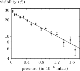
Two important sources of decoherence ubiquitous in nature were studied in a controlled fashion using fullerene interferometry experiments: collisional decoherence (see Sec. 4.1) [171, 170] and thermal decoherence [283]. To induce controlled collisional decoherence, the experiments by Hornberger et al. [171] and Hackermüller et al. [170] introduced a background gas of adjustable pressure into the interferometer. Scattering of gas molecules by the fullerenes creates entanglement, and which-path information about the fullerene is carried away by the gas molecules. The higher the gas pressure, the greater the likelihood for a fullerene to collide with a gas particle, and thus the stronger the resulting decoherence effect. Figure 17a shows the experimentally observed decrease of fringe visibility as a function of gas pressure, which was found to be in excellent agreement with theoretical models for collisional decoherence [57, 174]. The experimental data were also used to confirm the predictions of more realistic collisional-decoherence models based on the quantum linear Boltzmann equation [71, 132, 72, 73, 172, 74, 173, 12]. Moreover, as already mentioned in Sec. 4.1, Talbot–Lau interferometry is sensitive to molecular rotations [179, 180], and this observation has inspired the development of collisional-decoherence models that take into account both spatial and orientational decoherence of anisotropic molecules [181, 182, 183, 184, 185]; predictions derived from these models are in good agreement with experimental data [184].
To study decoherence of fullerenes due to emission of thermal radiation, Hackermüller et al. [283] used laser beams to heat the fullerene molecules to temperatures up to 3,000 K. Because the photons emitted from the heated molecules carry away which-path information, spatial coherence—and thus fringe visibility—is reduced. By changing the molecular temperature, the strength of the resulting thermal decoherence can be adjusted. Figure 17b shows the experimentally observed visibility of the interference fringes as a function of the laser heating power, with the corresponding (mean microcanonical) temperature of the molecular beam shown as well. We see that at temperatures below around 1,500 K (the source temperature is 900 K), thermal decoherence is still relatively weak and the fringe visibility is only mildly affected. Around 2,000 K, the decoherence becomes strong enough for interference fringes to start being visibly reduced, while around 2,500 K the visibility has been halved. Above 3,000 K, decoherence is complete and fringes are no longer discernible.
The observed dependence of the fringe visibility on molecular temperature is in good agreement with theoretical predictions [283]; see also Refs. [286, 287] for a detailed theoretical analysis of the experiment. To explain the temperature dependence [286], one notes that only above 2,000 K there is a non-negligible probability for a heated fullerene to emit a photon with a wavelength comparable to the extent of the spatial delocalization of the fullerene state (as given by the slit spacing ) such that appreciable which-path information can be obtained. Thus, this temperature marks the onset of decoherence. The emission of several photons of such wavelength is needed to cause a 50% decrease in fringe visibility, which requires the higher temperature regime of 2,500 K. Around 3,000 K, the average number of emitted photons per fullerene becomes large enough to produce full decoherence with no remaining fringe visibility. While for fullerene molecules substantial thermal decoherence obtains at only relatively high temperatures, for much larger molecules it becomes a significant source of decoherence even at room temperature, showing the importance of thermal decoherence for understanding the quantum-to-classical transition on macroscopic scales [8, 287, 9]. For example, observation of interference fringes for molecules on the order of amu (which is orders of magnitude beyond current experiments) would likely necessitate cooling the molecules to their vibrational ground state at below 77 K [12, 288].
6.3 Superconducting systems
Superconducting qubit systems, such as superconducting quantum interference devices (SQUIDs) and Cooper-pair boxes, play a prominent role in the exploration of coherence and decoherence in macroscopic systems. Their importance to fundamental studies of macroscopic quantum behavior was spelled out early by Leggett [289], who suggested, in 1980, that such systems may become ideal vehicles for the creation of cat-like superpositions of macroscopically distinct states. Superconducting qubits are also considered promising candidates for the realization of a quantum computer [290].
Superconductivity is a phenomenon in which pairs of electrons of opposite spin condense into a boson-like particle, known as a Cooper pair. Each Cooper pair is in a low-energy ground state. Provided the thermal vibrational energy of the crystal lattice of the material is lower than the energy gap between the ground and first excited states of the Cooper pair, interactions with the lattice cannot excite the Cooper pairs. The Cooper pairs can therefore freely move around the lattice, forming a resistance-free, persistent “supercurrent” whose collective center-of-mass motion may be described quantum-mechanically by a single, macroscopically extended wave function. When a thin insulating barrier between two pieces of superconducting material is inserted (known as a Josephson junction), Cooper pairs will tunnel through the barrier, leading to a flow of supercurrent even if no voltage is applied. This Josephson effect is a purely quantum-mechanical phenomenon (for reviews, see, e.g., Refs. [291, 292]).

Figure 18 schematically shows a SQUID with a single Josephson junction, a setup referred to as an rf-SQUID. The supercurrent creates an intrinsic magnetic flux threading the loop, and in addition an external magnetic field is applied to provide an adjustable external magnetic flux . The requirement that the macroscopic wave function around the loop must be continuous translates into a condition for the total trapped flux , which must obey , , where is the phase shift introduced by the Josephson junction and is the flux quantum. In this way, the total flux becomes quantized and serves as the single macroscopic variable representing the collective quantum-mechanical evolution of the Cooper pairs.
(a) (b)


The evolution of is effectively governed by a tilted double-well potential in flux space (Fig. 19a) [187], with the amount of tilt determined by the applied external flux, and resonant quantum tunneling between the wells may occur [295, 296]. Away from the bias point , each well contains low-lying energy eigenstates that are well-localized within each well, corresponding to approximate eigenstates of the flux operator. These localized eigenstates in a given well also approximately correspond to a macroscopic supercurrent flowing in a definite direction (clockwise or counterclockwise) around the loop. The two lowest-lying energy eigenstates are well-separated from higher-energy states, such that the SQUID effectively acts as a two-state system, forming a superconducting flux qubit.
At the bias point , the double-well potential becomes symmetric (Fig. 19b). The presence of the tunneling barrier leads to a level anticrossing that produces an energy ground state and a first excited state that are delocalized across the two wells. They are given by coherent superpositions of the states and (which are localized in each well) representing “classical” clockwise and counterclockwise supercurrents,
| (120a) | ||||
| (120b) | ||||
(a) (b)


Such superposition states of macroscopic supercurrents flowing in opposite directions were first observed in several experiments in the early 2000s [40, 41, 293, 294]. Friedman et al. [40] confirmed their existence indirectly through spectroscopic measurements of the energy splitting between them and found excellent agreement with theoretical predictions. The supercurrent in the experiment was several microampere. In experiments by Chiorescu et al. [293] (see Fig. 20a) and Ilichev et al. [294], the existence of the supercurrent superpositions was confirmed through the observation of Rabi oscillations between the states and (Fig. 20b).

The gradual loss of coherence from these supercurrent superpositions was first measured by Chiorescu et al. [293] using Ramsey interferometry. The SQUID was tuned close to the bias point and initialized in the ground state . A microwave pulse was applied to transform this state into an equal-weight superposition of and . The state was then allowed to evolve freely for a duration , followed by the application of a second microwave pulse. In the resulting state, occupation probabilities for the supercurrent states and will exhibit an oscillatory dependence on the delay time . This dependence was experimentally observed (see Fig. 21), with a measured frequency in excellent agreement with theoretical predictions. The characteristic time for the loss of phase coherence was obtained from the decay envelope of the oscillation and found to be around 20 ns. In subsequent experiments with superconducting flux qubits, various influences that limit coherence time were studied, including flux noise [297, 298] and photon noise [299]; in the latter experiment, relatively long coherence times of several microseconds were observed [299].
Loss of coherence has also been observed for superconducting charge qubits (Cooper-pair boxes [300]) and phase qubits. In a charge qubit, Cooper pairs tunnel through a Josephson junction onto a superconducting island, and the two qubit basis states are formed by states differing by the amount of charge on the island. Superpositions of such charge states were experimentally observed through Rabi oscillations [301] and coherent oscillations with a decay time of were measured [302]. For phase qubits, where the variable of interest is the phase difference between the electrodes of the Josephson junction, superpositions of macroscopically distinct phase states with coherence times up to several s have been observed [303, 304]. Since then, several improved designs of superconducting qubits, such as quantronium, transmon, and fluxonium qubits, have further enhanced the coherence time [290]. For example, a 3D transmon has achieved coherence times on the order of [305, 306].
Drawing on experimental data, a number of theoretical studies have investigated and modeled loss-of-coherence processes in superconducting qubits, focusing on sources such as intrinsic quasiparticle tunneling [307], the coupling to electromagnetic circuitry for SQUID readout [308], two-level defects in the Josephson junction [309], and fluctuations in the bias current of the Josephson junction [111]. Such investigations have indicated that many sources of an intrinsic loss of coherence in superconducting qubits may be modeled in terms of an environment composed of effective two-level systems [304, 309], i.e., by means of a spin–spin model (compare Sec. 4.4) [157, 156].
It should be noted here that in the aforementioned experimental and theoretical studies of superconducting qubits, the loss of coherence is typically due to ensemble dephasing induced by fluctuations (noise), rather than by an entanglement-based transfer of information to an environment. While phenomenologically the effect on the system’s density matrix may be similar for both processes, the physical differences between the two processes should be remembered; see the discussion in Sec. 2.6.
6.4 Ion traps
Ion traps are one of the most promising and advanced platforms for the implementation of a quantum computer [15]. The idea of using trapped ions for quantum computation goes back to the groundbreaking papers by Cirac and Zoller [310] and Monroe et al. [311]. The dynamics of trapped ions have been studied extensively [14]. Several quantum-computational tasks have been experimentally realized using ion-trap qubits, including demonstrations of the Deutsch–Jozsa algorithm [233], quantum teleportation [312, 313], quantum error correction [314], decoherence-free subspaces [227, 229, 230, 231], entanglement between several ions [315], and entanglement purification [316]; see Ref. [15] for a comprehensive review. In ion-trap qubits, ions are bound by a time-dependent potential (Paul trap [317, 14]), and the qubit states are formed by a pair of long-lived internal states of the ions [14, 15]. States of individual ions are typically initialized using optical-pumping techniques and are manipulated by laser pulses. Two-qubit operations may be carried out through coupling of collective motional degrees of freedom [310] or other means [15].
Many studies of the loss of coherence in ion traps have focused on dephasing caused by noise and fluctuations in the physical (and often classical) parameters describing the trapping and control of the ions (see, e.g., Refs. [121, 318, 319, 320, 321, 322, 15]). In fact, the influence of an environment is often simulated by actively driving fluctuations in parameters such as the trap frequency or by applying external noise [113, 121]. Since such loss of coherence is due to classical noise processes (manifesting their effect only in an ensemble average for which phase relations become smeared out) rather than entanglement-induced information transfer, the points discussed in Sec. 2.6 regarding the distinction between noise-induced and entanglement-induced decoherence should be kept in mind. A frequently used technique for measuring dephasing in ion traps is Ramsey interferometry, in much the same way as we have already discussed for photons in a cavity (Sec. 6.1) and superconducting qubits (Sec. 6.3).
Two different kinds of superposition states in ion traps should be distinguished: superpositions of the internal atomic levels that represent the qubit basis states, and superpositions of the motional states of the ions. Since superpositions of the internal qubit levels are merely microscopic, they are not in the territory of the mesoscopic and macroscopic “cat-like” superposition states we have discussed previously in the context of photon fields, matter-wave interferometry, and SQUIDs. For such trapped-ion qubit states, a dominant source of loss of coherence are fluctuations in the magnetic trapping field (see, e.g., Refs. [323, 319, 320, 15]). A superposition state of the ion will be sensitive to such fluctuations if its components differ in magnetic moment. Because the loss of coherence due to magnetic-field fluctuations has substantially limited achievable coherence times [15], several ion-trap experiments have used qubit states that have the same magnetic moment and that are therefore insensitive to fluctuations of the magnetic field (see, e.g., Refs. [324, 231, 325]). In this way, coherence times of 10 s for a superposition of two hyperfine levels in a single 9Be+ ion have been achieved [231] (see Fig. 22). Other fluctuations in the experimental parameters that lead to a loss of coherence arise in the context of the control of the ion, for example, in the form of fluctuations in the intensity [109] and duration [110] of the laser beam, off-resonant excitations [326], AC-Stark shifts [327], and detuning errors [328].
Let us now turn to the second kind of superposition states relevant to ion traps, namely, superpositions of motional states. Provided proper tuning of the trap parameters, the motion of a trapped ion is equivalent to that of a quasi-one-dimensional harmonically bound particle, and therefore the motional state of the ion may be represented by a harmonic oscillator [14, 329]. From a practical point of view, motional states of trapped ions are important because in certain implementations of ion-trap qubits, two-qubit gate operations are implemented by storing quantum information in motional states [310]. Different motional superposition states have been realized experimentally, including superpositions of coherent states [330, 113, 121, 329] and Fock states (i.e., number eigenstates) [113, 121], and their dephasing has been observed [113, 121, 323]. In 1996, Monroe et al. [330] reported the observation of an ion for which the internal spin states and were quantum-correlated (entangled) with two coherent motional states and representing wave packets oscillating back and forth in the trap potential,
| (121) |
In the experiment, , so the motions of the wave packets were out of phase with each other; the maximum separation between the two wave packets at the turning points was 83 nm, with a wave-packet size of 7.1 nm.

Dephasing of such states was experimentally studied by Turchette et al. [121] using Ramsey interferometry (see Fig. 23). The authors simulated a dephasing environment by varying the trap frequency during the wait time between the two Ramsey pulses, which introduced a relative phase shift between the components in the superposition. The frequency was changed adiabatically to avoid energy transfer to and from the ion. The loss of coherence then appears as the result of an averaging over many different instances of the random noise process. It is therefore to be understood as a consequence of ensemble averaging, rather than entanglement with an environment (see again Sec. 2.6 for comments on this distinction). Superpositions of Fock states, with number differences up to , and their dephasing were also observed. In a different experiment, Schmidt-Kaler et al. [323] measured motional center-of-mass-mode coherence times on the order of 100 ms for a trapped 40Ca+ ion described by a superposition of two vibrational states.
(a) (b) (c)

Ion traps have also been used to experimentally explore the dynamics of entanglement under the influence of an environment. For example, Barreiro et al. [251] reported an experiment in which four entangled trapped-ion qubits were coupled to an engineered, tunable environment. By varying the amount of dephasing (represented by a parameter ) introduced into the multiparticle system and then tomographically reconstructing the resulting state, crossovers between different entanglement regimes were observed (see Fig. 24). In the absence of dephasing (), the entangled multiparticle state was shown to violate a Bell–CHSH inequality. With even a relatively small amount of dephasing (), the state no longer violates the inequality. Around , the state crosses over into bound entanglement [331], i.e., it becomes a state that is entangled but not distillable. Around , the state becomes completely separable, indicating that all entanglement initially present in the multiparticle state has been lost to dephasing.
As already discussed in Sec. 5.1, trapped ions have also been used in experimental studies of decoherence-free subspaces [227, 229, 230, 231], reservoir engineering [237, 113, 121, 238] (of which the aforementioned studies by Turchette et al. [121] are an example), and quantum state engineering [239, 240, 241].
6.5 Other experimental areas
We shall very briefly list a few other existing and prospective areas for the observation of decoherence.
Quantum dots
Mechanical quantum resonators
Mechanical quantum resonators [339, 340, 341, 342], coupled either to electronic transducers (“quantum electromechanical systems” [342, 340, 341]) or photon fields (“cavity optomechanical systems” [339]), are promising candidates for the generation of spatial macro-superpositions [263]. Such resonators may be effectively treated, under the right conditions, as a one-dimensional quantum harmonic oscillator, which represents the fundamental flexural mode. Several potential decoherence mechanisms have been explored. For example, the role of intrinsic tunneling two-level defects (i.e., spin- particles) as a decohering (and dissipative) environment has been studied [343, 344, 342, 345, 346, 347, 348, 349, 196, 339], including consideration of decoherence models in which the resonator interacts with a collection of two-level systems that are in turn subject to a decohering bosonic bath [196, 349]. While decoherence in quantum resonators has often been investigated in the context of dissipative processes such as heating (see, e.g., Refs. [343, 344, 346, 347, 348, 339]), pure dephasing has also been observed and analyzed [350, 351, 352, 353, 354]. For example, Ref. [354] experimentally studied dephasing of a resonator due to a simulated phase reservoir, realized by inducing fluctuations in the resonator frequency through applied voltage noise.
Bose–Einstein condensates
Different kinds of superposition states and nonclassical phenomena have been observed in Bose–Einstein condensates, including: interference fringes between independent, overlapping condensates arising from the indistinguishability of bosons [355]; interference between single atoms in a coherently split condensate involving either spatial or internal degrees of freedom (see, e.g., Refs. [356, 357]); and many-particle entanglement [358, 359, 360]. For Bose–Einstein condensates described by a superposition of macroscopically different particle numbers (see, e.g., Refs. [361, 362, 363, 364, 365, 366, 367]), collisional decoherence due to scattering processes between condensate and noncondensate atoms has been studied theoretically [236]. Decoherence of phonons representing the collective quantum excitations of the condensate atoms in an isolated Bose–Einstein condensate has also been modeled [368]. Ref. [369] considered the coherent splitting of a Bose–Einstein condensate into two distinct momentum modes traversing a Mach–Zehnder-like interferometer, such that the accumulated phase difference between the two arms of the interferometer leads to an interference signal at the output. The authors investigated the susceptibility of this interference signal to decoherence processes, as well as to hypothetical collapse theories such as continuous spontaneous localization models [370, 371, 372].
6.6 Prospective tests of quantum mechanics
Decoherence experiments are also useful for testing the universal validity of quantum mechanics [13, 373, 374, 375, 263, 376, 288, 377], most notably with respect to the hypothetical presence of a novel nonunitary mechanism in nature that would break the linearity of the Schrödinger time evolution and lead to wave-function collapse. Such mechanisms that modify the linear structure of quantum mechanics are known under the headings of collapse theories, dynamical reduction models, and continuous spontaneous localization models; see Ref. [370] for a comprehensive review. As long as the observable effect of such nonlinearities is to effectively destroy or prevent quantum interferences, the challenge is to distinguish such effects from those produced by ordinary quantum decoherence [371, 372]. One would need to sufficiently shield the system from decoherence in order to unambiguously isolate the postulated reduction effect. This goal is difficult to achieve, because for the collapse mechanism to become appreciable, the size of the system must be sufficiently large, in which case decoherence will in general be strong as well [178, 378].
The superpositions realized in current experiments are still not sufficiently macroscopic to rule out collapse theories, although it has been demonstrated [175] that matter-wave interferometry with large molecular clusters (in the mass range between and ) would be able to test the collapse theories proposed in Refs. [371, 372]; such experiments may soon become technologically feasible [12, 263]. Other promising avenues for testing quantum mechanics include motional superposition states of micromechanical oscillators [373, 375], interference of free nanoparticles [379, 376] (an approach that offers the prospect of spatial superpositions separated by 100 nm for particles on the order of [376]), and molecular nanorotors [377]. Ultimately, experiments carried out in space rather than on Earth might be able to push the limit for macroscopic superpositions to objects involving on the order of atoms [288]. In such space-based experiments, low background gas pressures () would minimize collisional decoherence, low temperatures () would minimize thermal decoherence, and microgravity () would minimize decoherence induced by gravitational time dilation [380], potentially enabling tests of quantum gravity models [288].
A related issue of interest is the question of how one may best quantify the “catness”—i.e., the macroscopicity or “size”—of a given superposition state. Various measures of macroscopicity have been suggested [289, 13, 385, 386, 387, 388, 389, 390, 378]. Most are focused on analyzing particular representations of quantum states and rely on quantum-information-theoretic measures such as the quantum Fisher information [390]. Such approaches tend to depend on particular basis choices for the decomposition of the wave function and can make it difficult to compare macroscopicities of states between physically different systems. Nimmrichter and Hornberger [378] have introduced an alternative measure of macroscopicity that quantifies the extent to which a given superposition state would be capable of ruling out small modifications of quantum mechanics. To represent such a modification in the most general and model-independent way, the authors considered a dynamical-semigroup framework in which a dynamical generator obeying certain invariance and symmetry conditions is added to the evolution equation for the density operator of an -particle system such that superpositions of macroscopically distinct states are dynamically transformed into classical mixtures. Specific collapse models, such as continuous spontaneous localization models [370], may be recovered as special cases within this framework. The effect of the modification can be quantified in terms of the resulting coherence time of the superposition, leading to the definition of a corresponding macroscopicity parameter [378]. Figure 25 shows estimates of for several existing and prospective experiments. One sees that, by this measure, the spatial superpositions involved in matter-wave interferometry (see Sec. 6.2) exhibit some of the largest macroscopicity; the aforementioned proposed experiments on free nanoparticles [379, 376] and micromechanical oscillators [373, 375] would also rank high on the macroscopicity scale.
7 Decoherence and the foundations of quantum mechanics
Since the early days of quantum mechanics, the interpretation of the quantum formalism and its attending foundational questions have been the subject of much debate (see, for example, Bacciagaluppi and Valentini’s analysis of the 1927 Solvay conference [391]). Especially given that decoherence theory was “discovered” only relatively recently, it is natural to ask what role decoherence may play in addressing foundational problems and informing the existing interpretations of quantum mechanics. One of the central topics in the foundations of quantum mechanics is known as the quantum measurement problem [392, 393, 394, 6, 395, 396], and in Sec. 7.1 we will discuss whether decoherence has anything of substance to say about it. In Sec. 7.2, we will then briefly review the role that decoherence plays, or may play, in the various interpretations of quantum mechanics. In Sec. 7.3, we will comment on Niels Bohr’s views on the primacy of classical concepts and their relationship to the quantum–classical correspondence described by decoherence. For in-depth discussions of the connections between decoherence and the foundations of quantum mechanics, see, for example, Refs. [7, 6, 397, 9]. Looking beyond the subject of decoherence, the interviews collected in Ref. [396] provide an overview of contemporary attitudes toward the interpretation of quantum mechanics.
7.1 Decoherence and the measurement problem
Application of the unitary Schrödinger evolution to a measuring apparatus interacting with a system prepared in a quantum superposition state cannot dynamically describe the stochastic selection of a particular term in the superposition as the measurement outcome (the “collapse of the wave function”); rather, system and apparatus end up in an entangled state, with all terms of the original superposition still present and quantum-correlated with different apparatus states. This is the measurement problem: the question of how to reconcile the linear, deterministic evolution described by the Schrödinger equation with our observation of the occurrence of random measurement outcomes. Whether one considers the measurement problem a genuine difficulty depends strongly on one’s interpretation of quantum states (see Ref. [396] for a representation of different views on the issue). Generally, the need to supply a dynamical account of the reduction of the superposition to a single outcome in the course of a measurement is much more acute when the quantum state is construed as a real, physical entity, rather than as encapsulating an observer’s information or beliefs. (The latter, “epistemic” view is most radically, and consistently, realized in the QBist interpretation of quantum mechanics [65], in which quantum states represent an observer’s beliefs—his probabilistic expectations—about his future experiences resulting from his interactions with the system.)
The measurement problem as just defined cannot be solved by decoherence [6, 9]. This is so for two reasons. First, the dynamics of decoherence processes are based entirely on the standard, unitary Schrödinger evolution. Second, the predictively relevant part of decoherence theory relies on reduced density matrices, which are derived from the requirement that they encode the correct quantum statistics (expectation values) for all measurements pertaining to only a subset of degrees of freedom of a composite system in a multipartite (and in general entangled) state. This derivation presumes the existence and validity of the usual measurement axioms of quantum mechanics, in particular, the collapse postulate and Born’s rule. In other words, for the kinds of entangled quantum states produced by decoherence-type interactions to be interpreted as describing a situation in which the system becomes “classical,” we need to take the existence of measurement outcomes as a priori given, or otherwise give an account outside of decoherence of how measurement outcomes are produced, because the property of classicality is ultimately a statement about measurement statistics. Thus decoherence, by itself, cannot address the measurement problem in any substantial way.
Of course, to say that decoherence has no bearing on the measurement problem—or on any of the “big” foundational problems in general—is not to suggest that decoherence and its underlying ideas cannot be of relevance in the investigation of fundamental questions. In fact, to give just one example, further explorations of the role of the environment, such as those undertaken in the development of quantum Darwinism (see Sec. 2.5), have already shed valuable light on deeper issues concerning information transfer, amplification, irreversibility, and communication in the quantum setting [87, 88, 89, 90, 91, 92, 93, 94, 95, 104, 398, 399, 99] (see Ref. [92] for an overview of some of the relevant ideas).
If one takes the quantum measurement problem to include the preferred-basis problem [9], and if the preferred-basis problem is understood in the sense defined in Sec. 2.4, then decoherence solves it, as discussed there. Indeed, the ability of decoherence to dynamically define preferred bases is exploited in certain interpretations of quantum mechanics (see the following Sec. 7.2).
7.2 Decoherence in interpretations of quantum mechanics
The interplay between decoherence and the interpretation of quantum mechanics goes back to the birth of decoherence. As mentioned in the Introduction, decoherence theory itself initially came about all but as a by-product of Zeh’s development of an interpretation in the mold of Everett’s many-worlds interpretation [1]. Since then, various interpretations have been assessed and refined in light of the insights and results brought about by the decoherence program. Most notably, decoherence has been used to define certain structural elements in interpretations, as well as identify internal consistency issues. Below, we shall give just give a few examples; the interested reader is pointed to Refs. [6, 7] for in-depth discussions of the interplay between decoherence and interpretations.
In Everett-style “many worlds” interpretations of quantum mechanics [49, 400], the quantum state is interpreted realistically and never collapses; our observation of definite measurement outcomes is then explained as a continuous “branching” of universes, worlds, observers, and minds in the course of measurement-like interactions. Another version, which arguably includes Everett’s own conception, interprets the global entangled state as merely describing relations between states (“relative-state interpretation”); see also Refs. [401, 402]. The preferred-basis problem is particularly acute in such interpretations, since the particular decomposition of the global quantum state (representing, in principle, the entire universe) defines the “worlds” (or “relations”) and thus their properties at each instant in time; those worlds must also be appropriately connected in time. Here, the pointer states defined by the stability criterion of decoherence (see Sec. 2.4) provide a ready-made solution, and in this way decoherence theory has played a critical role in defining the branching structure in Everett-style interpretations [84, 403, 404, 405, 400]. Such an approach does not need to define the worlds a priori or by means of an external rule; instead, the worlds are defined dynamically through the standard Schrödinger evolution, and since they are dynamically stable, they lead to robust, temporally extended trajectory-like branches. A relative-state interpretation that draws heavily from the insights and structures provided by decoherence theory is the “existential interpretation” of Zurek [82, 84, 406]. This interpretation was later extended to include the results of quantum Darwinism [92], as well as a decoherence-inspired account of the origin of Born’s rule based on symmetry and invariance properties of entangled system–environment states (“environment-assisted invariance”) [5, 407, 87, 406, 92, 99, 408, 409, 410].
In modal interpretations of quantum mechanics [411], the physical quantity represented by an observable may be assigned a definite value even if the system is not in an eigenstate of that observable. The assignment of such definite values (corresponding to well-defined physical properties) must be in agreement with the prediction of quantum mechanics; in particular, the proper Born probabilities and time evolution must be recovered. Also, at least on macroscopic scales the modally assigned definite values ought to correspond to the definite “classical” quantities of our experience, such as well-localized positions. Recognizing the importance of environmental interactions highlighted by decoherence theory, some modal interpretations have derived their value assignments from states obtained from an orthogonal decomposition of the decohered reduced density matrix [412, 413]. For finite-dimensional state spaces, the resulting states are found to be very close to the states that would be dynamically selected by the stability criterion of decoherence, ensuring proper classicality of the modally assigned properties [412, 413]. For infinite-dimensional state spaces, however, this agreement often breaks down; for example, for an environmental-scattering model it was shown that the modal properties obtained from the orthogonal decomposition of the decohered reduced density matrix were significantly delocalized while the pointer states indicated tight localization [414]. Such inconsistencies can pinpoint limitations and empirical inadequacies of certain types of modal interpretations.
The consistent-histories interpretation of quantum mechanics [415, 416, 417] dispenses with the usual notions of measurement and instead defines time-ordered sequences of events (“histories”) for a closed system and assigns appropriate probabilities to these sequences. As a minimal requirement, such sets of histories must fulfill a consistency condition [415, 416, 417] to ensure the applicability of Boolean logic in the form of the additivity of probabilities. This, however, is not enough, as most consistent histories do not exhibit appropriate quasiclassicality for macroscopic systems [418, 419, 82, 420, 421, 422, 423]. To address this issue, the pointer bases obtained from decoherence have frequently been used to dynamically yield consistent, quasiclassical histories [82, 420, 424, 421, 425], and the importance of “records” (represented by stable system–environment correlations) for the definition of quasiclassical histories has been emphasized repeatedly [424, 421, 420, 82, 5, 426]. In particular, the redundant environmental encoding of such records, as described by quantum Darwinism, has been identified as a key mechanism for ensuring consistent, stable, quasiclassical, objective histories [427] (see also Refs. [82, 420, 5, 87]).
7.3 Bohr’s views on the primacy of classical concepts
In Niels Bohr’s writings on quantum mechanics, the indispensability and primacy of “classical concepts” (such as position and momentum) is widely emphasized (see, for example, Refs. [428, 429, 430, 431, 432, 433]). Indeed, Howard has stated that “the doctrine of classical concepts turns out to be more fundamental to Bohr’s philosophy of physics than are better-known doctrines, like complementarity” [434, p. 202]. Given that decoherence theory describes a dynamical emergence of classicality, it is not surprising that decoherence has sometimes been suggested to make Bohr’s insistence on fundamental classical concepts superfluous. For example, Joos has traced the birth of the ideas of decoherence theory to a dissatisfaction with the “orthodoxy of the Copenhagen school” [435, p. 54]. He has argued that “the message of decoherence” is that “we do not need to take classical notions as the starting point for physics,” because “these emerge through the dynamical process of decoherence from the quantum substrate” [435, p. 77]. Similarly, Zeh [436] has asserted that
the Heisenberg–Bohr picture of quantum mechanics can now be claimed dead. Neither classical concepts, nor any uncertainty relations, complementarity, observables, quantum logic, quantum statistics, or quantum jumps have to be introduced on a fundamental level.
Any analysis of such claims is complicated by the variety of meanings of the term “classical”—referring variously to concepts, dynamical properties, statistics, phenomena, laws, or theories. A closer reading of Bohr’s views reveals that his insistence on the primacy of classical concepts is chiefly grounded in epistemological concerns, and that it pertains to his understanding of the functional role of experiments [19, 437]. For Bohr, classical concepts are indispensable because without them, it would impossible to acquire empirical knowledge of the world through experiments. Therefore, according to Bohr, any interpretation of quantum mechanics must in the end fall back on the use of classical concepts, rendering circular any attempt to derive such concepts from the quantum formalism. This suggests that we must clearly distinguish between Bohr’s epistemological thesis of the primacy of classical concepts based on his view of the functional role of an experiment, and the dynamical problem of the quantum–classical transition. It is the latter that is addressed by decoherence theory, not the former [19, 437].
While Bohr repeatedly emphasized the epistemological necessity of classical concepts, he offered only a few oblique comments on the problem of why, physically and dynamically, macroscopic systems and measurement apparatuses may be described in classical terms. These comments mostly involved the “heaviness” and large size of macroscopic systems, though they frequently also referred to irreversible amplification effects (see, e.g., Refs. [433, 438]); for example, with regard to measurement apparatuses Bohr stated that they “concern bodies sufficiently heavy to permit the quantum [effects] to be neglected in their description” [433, p. 170].
Heisenberg, in a tantalizing passage, wrote that [439, pp. 121–2]
the system which is treated by the methods of quantum mechanics is in fact a part of a much bigger system (eventually the whole world); it is interacting with this bigger system; and one must add that the microscopic properties of the bigger system are (at least to a large extent) unknown. …The interaction with the bigger system with its undefined microscopic properties then introduces a new statistical element into the description … of the system under consideration. In the limiting case of the large dimensions this statistical element destroys the effects of the “interference of probabilities” in such a manner that the quantum-mechanical scheme really approaches the classical one in the limit.
In a similar vein, elsewhere Heisenberg suggested that “the interference terms are … removed by the partly undefined interactions of the measuring apparatus, with the system and with the rest of the world” [440, p. 23]. Even though one might identify a faint hint of the later ideas of the decoherence program in Heisenberg’s pronouncements, there is no mention of the critical ingredient: entanglement.
In the 1950s and 1960s, several of Bohr’s disciples, including Weizsäcker and Rosenfeld, attempted to develop a physical account of the quantum-to-classical transition based on notions of irreversibility, a strategy they saw as serving as a dynamical justification of Bohr’s classical concepts [19]. The thermodynamic theory of Daneri, Loinger, and Prosperi [441], which built on Bohr’s hints concerning the role of irreversibility and amplification, is perhaps the best known (though circular [442, 443]) approach. Yet, none of these early efforts recognized the role of entanglement in a dynamical explanation of quantum statistics turning into classical-looking distributions.
8 Concluding remarks
Schrödinger called entanglement “the characteristic trait of quantum mechanics, the one that enforces its entire departure from classical lines of thought” [444, p. 555]. He used his eponymous cat paradox to argue how entanglement amplified to macroscopic scales demonstrates the apparent irreconcilability of quantum mechanics with our “classical” experience of the everyday world. On this view, entanglement was perceived to be a peculiar quantum feature that would have to be tamed in order to bridge the gap between quantum and classical descriptions. So it is perhaps ironic that entanglement turned out to be the key to a dynamical explanation of the emergence of classicality in quantum mechanics.
Without a doubt, future experiments will realize ever-larger Schrödinger cat–like states, and we will continue our journey toward the realization of a quantum computer. A key role in all such endeavors will be played by a deep understanding of decoherence and an ongoing development of decoherence models of increasing complexity and detail. It is indeed remarkable how the basic idea of decoherence—that entanglement of a quantum system with an environment has a dramatic influence on what is observable at the level of the system, an idea already spelled out in the very first paper by Zeh [1]—has enriched so thoroughly our theoretical understanding and experimental control of the quantum-to-classical transition.
We shall close with a quote by Zeh himself, who not only was a pioneer of decoherence theory but remained, for the rest of his life, a steadfast, thoughtful advocate of the inseparability of his discovery from the interpretation of quantum mechanics. In 1996, he humbly observed [445] that decoherence is
a normal consequence of interacting quantum mechanical systems. It can hardly be denied to occur—but it cannot explain anything that could not have been explained before. Remarkable is only its quantitative (realistic) aspect that seems to have been overlooked for long.
References
- [1] H. D. Zeh, On the interpretation of measurement in quantum theory, Found. Phys. 1 (1970) 69–76.
- [2] W. H. Zurek, Pointer basis of quantum apparatus: Into what mixture does the wave packet collapse?, Phys. Rev. D 24 (1981) 1516–1525.
- [3] W. H. Zurek, Environment-induced superselection rules, Phys. Rev. D 26 (1982) 1862–1880.
- [4] J. P. Paz, W. H. Zurek, Environment-induced decoherence and the transition from quantum to classical, in: R. Kaiser, C. Westbrook, F. David (Eds.), Coherent Atomic Matter Waves, Les Houches Session LXXII, Vol. 72 of Les Houches Summer School Series, Springer, Berlin, 2001, pp. 533–614.
- [5] W. H. Zurek, Decoherence, einselection, and the quantum origins of the classical, Rev. Mod. Phys. 75 (2003) 715–775.
- [6] M. Schlosshauer, Decoherence, the measurement problem, and interpretations of quantum mechanics, Rev. Mod. Phys. 76 (2004) 1267–1305.
- [7] G. Bacciagaluppi, The role of decoherence in quantum mechanics, in: E. N. Zalta (Ed.), The Stanford Encyclopedia of Philosophy, 2012, online at http://plato.stanford.edu/archives/win2012/entries/qm-decoherence.
- [8] E. Joos, H. D. Zeh, C. Kiefer, D. Giulini, J. Kupsch, I.-O. Stamatescu, Decoherence and the Appearance of a Classical World in Quantum Theory, 2nd Edition, Springer, New York, 2003.
- [9] M. Schlosshauer, Decoherence and the Quantum-to-Classical Transition, Springer, Berlin/Heidelberg, 2007.
- [10] E. Schrödinger, Die gegenwärtige Situation in der Quantenmechanik, Naturwissenschaften 23 (1935) 807–812, 823–828, 844–849.
- [11] J. M. Raimond, M. Brune, S. Haroche, Manipulating quantum entanglement with atoms and photons in a cavity, Rev. Mod. Phys. 73 (2001) 565–582.
- [12] K. Hornberger, S. Gerlich, S. Nimmrichter, P. Haslinger, M. Arndt, Colloquium: Quantum interference with clusters and molecules, Rev. Mod. Phys. 84 (2012) 157–173.
- [13] A. J. Leggett, Testing the limits of quantum mechanics: motivation, state of play, prospects, J. Phys.: Condens. Matter 14 (2002) R415–R451.
- [14] D. Leibfried, R. Blatt, C. Monroe, D. Wineland, Quantum dynamics of single trapped ions, Rev. Mod Phys. 75 (2003) 281–324.
- [15] H. Häffner, C. F. Roos, R. Blatt, Quantum computing with trapped ions, Phys. Rep. 469 (2008) 155–203.
- [16] D. A. Lidar, T. A. Brun (Eds.), Quantum Error Correction, Cambridge University Press, 2013.
- [17] K. Camilleri, A history of entanglement: Decoherence and the interpretation problem, Stud. Hist. Phil. Mod. Phys. 40 (2009) 290–302.
- [18] E. Joos, Elements of environmental decoherence, in: P. Blanchard, D. Giulini, E. Joos, C. Kiefer, I.-O. Stamatescu (Eds.), Decoherence: Theoretical, Experimental, and Conceptual Problems, Springer, Berlin, 2000, pp. 1–17.
- [19] K. Camilleri, M. Schlosshauer, Niels Bohr as philosopher of experiment: Does decoherence theory challenge Bohr’s doctrine of classical concepts?, Stud. Hist. Phil. Mod. Phys. 49 (2015) 73–83.
- [20] O. Kübler, H. D. Zeh, Dynamics of quantum correlations, Ann. Phys. (N.Y.) 76 (1973) 405–418.
- [21] E. Joos, H. D. Zeh, The emergence of classical properties through interaction with the environment, Z. Phys. B: Condens. Matter 59 (1985) 223–243.
- [22] W. H. Zurek, Reduction of the wavepacket: How long does it take?, in: G. T. Moore, M. O. Scully (Eds.), Frontiers of Nonequilibrium Statistical Mechanics, Plenum Press, New York, 1986, pp. 145–149, first published in 1984 as Los Alamos report LAUR 84-2750.
- [23] D. F. Walls, G. J. Milburn, Effect of dissipation on quantum coherence, Phys. Rev. A 31 (1985) 2403–2408.
- [24] D. F. Walls, M. J. Collett, G. J. Milburn, Analysis of quantum measurement, Phys. Rev. D 32 (1985) 3208–3215.
- [25] A. O. Caldeira, A. J. Leggett, Influence of damping on quantum interference: An exactly soluble model, Phys. Rev. A 31 (1985) 1059–1066.
- [26] W. H. Zurek, Decoherence and the transition from quantum to classical, Phys. Today 44 (1991) 36–44, see also the updated version available as eprint quant-ph/0306072.
- [27] R. P. Feynman, Simulating physics with computers, Int. J. Theor. Phys. 21 (1982) 467–488.
- [28] D. Deutsch, Quantum theory, the Church–Turing principle and the universal quantum computer, Proc. R. Soc. Lond. A 400 (1985) 97–117.
- [29] D. Deutsch, R. Jozsa, Rapid solution of problems by quantum computation, Proc. R. Soc. Lond. A 439 (1992) 553–558.
- [30] A. Berthiaume, G. Brassard, Oracle quantum computing, in: Proc. Workshop on Physics of Computation: PhysComp ’92, IEEE Computer Society Press, Los Alamitos, CA, 1992, pp. 60–62.
- [31] A. Berthiaume, G. Brassard, The quantum challenge to structural complexity theory, in: Proc. 7th Annual Structure in Complexity Theory Conf., IEEE Computer Society Press, Los Alamitos, CA, 1992, pp. 132–137.
- [32] E. Bernstein, U. Vazirani, Quantum complexity theory, in: Proceedings of the 25th Annual ACM Symposium on Theory of Computing, ACM, New York, 1993, pp. 11–20.
- [33] D. Simon, On the power of quantum computation, in: Proc. 35th Annual Symp. on Foundations of Computer Science, IEEE Computer Society Press, Los Alamitos, CA, 1994, pp. 124–134.
- [34] P. W. Shor, Polynomial-time algorithms for prime factorization and discrete logarithms on a quantum computer, in: Proceedings of the 35th Annual Symposium on the Foundations of Computer Science, IEEE Computer Society Press, Los Alamitos, CA, 1994, pp. 124–134.
- [35] P. W. Shor, Polynomial-time algorithms for prime factorization and discrete logarithms on a quantum computer, SIAM J. Comp. 26 (1997) 1484–1509.
- [36] L. K. Grover, A fast quantum mechanical algorithm for database search, in: Proc. of the 28th Annual ACM Symposium on the Theory of Computing, ACM, New York, 1996, pp. 212–219.
- [37] L. K. Grover, Quantum mechanics helps in search for a needle in a haystack, Phys. Rev. Lett. 79 (1997) 325–328.
- [38] M. Brune, E. Hagley, J. Dreyer, X. Maître, A. Maali, C. Wunderlich, J. M. Raimond, S. Haroche, Observing the progressive decoherence of the “meter” in a quantum measurement, Phys. Rev. Lett. 77 (1996) 4887–4890.
- [39] M. Arndt, O. Nairz, J. Vos-Andreae, C. Keller, G. van der Zouw, A. Zeilinger, Wave–particle duality of C60 molecules, Nature 401 (1999) 680–682.
- [40] J. R. Friedman, V. Patel, W. Chen, S. K. Yolpygo, J. E. Lukens, Quantum superposition of distinct macroscopic states, Nature 406 (2000) 43–46.
- [41] C. H. van der Wal, A. C. J. ter Haar, F. K. Wilhelm, R. N. Schouten, C. J. P. M. Harmans, T. P. Orlando, S. Lloyd, J. E. Mooij, Quantum superposition of macroscopic persistent-current states, Science 290 (2000) 773–777.
- [42] K. Hornberger, Introduction to decoherence theory, in: A. Buchleitner, C. Viviescas, M. Tiersch (Eds.), Entanglement and Decoherence: Foundations and Modern Trends, Vol. 768 of Lecture Notes in Physics, Springer, Berlin, 2009, pp. 221–276.
- [43] H.-P. Breuer, F. Petruccione, The Theory of Open Quantum Systems, Oxford University Press, Oxford, 2002.
- [44] W. K. Wootters, W. H. Zurek, Complementarity in the double-slit experiment: Quantum nonseparability and a quantitative statement of Bohr’s principle, Phys. Rev. D 19 (1979) 473–484.
- [45] B.-G. Englert, Fringe visibility and which-way information: An inequality, Phys. Rev. Lett. 77 (1996) 2154–2157.
- [46] L. D. Landau, The damping problem in wave mechanics, Z. Phys. 45 (1927) 430–441.
- [47] J. von Neumann, Mathematische Grundlagen der Quantenmechanik, Springer, Berlin, 1932.
- [48] W. H. Furry, Note on the quantum mechanical theory of measurement, Phys. Rev. 49 (1936) 393–399.
- [49] H. Everett, “Relative state” formulation of quantum mechanics, Rev. Mod. Phys. 29 (1957) 454–462.
- [50] A. Einstein, B. Podolsky, N. Rosen, Can quantum-mechanical description of physical reality be considered complete?, Phys. Rev. 47 (1935) 777–780.
- [51] J. S. Bell, On the Einstein–Podolsky–Rosen paradox, Physics 1 (1964) 195–200.
- [52] J. S. Bell, On the problem of hidden variables in quantum mechanics, Rev. Mod. Phys. 38 (1966) 447–452.
- [53] A. Peres, Unperformed experiments have no results, Am. J. Phys. 46.
- [54] J. P. Paz, S. Habib, W. H. Zurek, Reduction of the wave packet: Preferred observable and decoherence time scale, Phys. Rev. D 47 (1993) 488–501.
- [55] A. J. Leggett, S. Chakravarty, A. T. Dorsey, M. P. A. Fisher, A. Garg, Dynamics of the dissipative two-state system, Rev. Mod. Phys. 59 (1987) 1–85.
- [56] S. G. Mokarzel, A. N. Salgueiro, M. C. Nemes, Modeling the reversible decoherence of mesoscopic superpositions in dissipative environments, Phys. Rev. A 65 (2002) 044101.
- [57] K. Hornberger, J. E. Sipe, Collisional decoherence reexamined, Phys. Rev. A 68 (2003) 012105.
- [58] K. Kraus, General state changes in quantum theory, Ann. Phys. 64 (1971) 311–355.
- [59] K. Kraus, States, Effects, and Operations, Springer, Berlin, 1983.
- [60] R. Alicki, K. Lendi, Quantum Dynamical Semigroups and Applications, 2nd Edition, Vol. 717 of Lect. Notes Phys., Springer, Berlin/Heidelberg, 2007.
- [61] J. von Neumann, Thermodynamik quantummechanischer Gesamheiten, Gött. Nach. 1 (1927) 273–291.
- [62] B. d’Espagnat, Two remarks on the theory of measurement, Nuovo Cimento Suppl. 1 (1966) 828–838.
- [63] B. d’Espagnat, Conceptual Foundations of Quantum Mechanics, 2nd Edition, Benjamin, Reading, Massachusetts, 1976.
- [64] B. d’Espagnat, Veiled Reality, an Analysis of Present-Day Quantum Mechanical Concepts, Addison-Wesley, Reading, Massachusetts, 1995.
- [65] C. A. Fuchs, N. D. Mermin, R. Schack, An introduction to QBism with an application to the locality of quantum mechanics, Am. J. Phys. 82 (2014) 749–754.
- [66] E. Wigner, On the quantum correction for thermodynamic equilibrium, Phys. Rev. 40 (1932) 749–759.
- [67] M. Hillery, R. F. O’Connell, M. O. Scully, E. P. Wigner, Distribution functions in physics: Fundamentals, Phys. Rep. 106 (1984) 121–167.
- [68] R. L. Hudson, When is the Wigner quasi-probability density non-negative?, Rep. Math. Phys. 6 (1974) 249–252.
- [69] M. R. Gallis, G. N. Fleming, Environmental and spontaneous localization, Phys. Rev. A 42 (1990) 38–48.
- [70] L. Diósi, Quantum master equation of a particle in a gas environment, Europhys. Lett. 30 (1995) 63–68.
- [71] K. Hornberger, Master equation for a quantum particle in a gas, Phys. Rev. Lett. 97 (2006) 060601.
- [72] K. Hornberger, B. Vacchini, Monitoring derivation of the quantum linear Boltzmann equation, Phys. Rev. A 77 (2008) 022112.
- [73] M. Busse, K. Hornberger, Emergence of pointer states in a non-perturbative environment, J. Phys. A: Math. Theor. 42 (2009) 362001.
- [74] M. Busse, K. Hornberger, Pointer basis induced by collisional decoherence, J. Phys. A: Math. Theor. 43 (2010) 015303.
- [75] R. A. Harris, L. Stodolsky, On the time dependence of optical activity, J. Chem. Phys. 74 (1981) 2145–2155.
- [76] H. D. Zeh, The meaning of decoherence, in: P. Blanchard, D. Giulini, E. Joos, C. Kiefer, I. Stamatescu (Eds.), Decoherence: Theoretical, Experimental, and Conceptual Problems, Lecture Notes in Physics No. 538, Springer, Berlin, 2000, pp. 19–42.
- [77] J. Trost, K. Hornberger, Hund’s paradox and the collisional stabilization of chiral molecules, Phys. Rev. Lett. 103 (2009) 023202. doi:10.1103/PhysRevLett.103.023202.
- [78] M. Bahrami, A. Shafiee, A. Bassi, Decoherence effects on superpositions of chiral states in a chiral molecule, Phys. Chem. Chem. Phys. 14 (2012) 9214–9218.
- [79] D. Giulini, C. Kiefer, H. D. Zeh, Symmetries, superselection rules, and decoherence, Phys. Lett. A 199 (1995) 291–298.
- [80] D. Giulini, Decoherence: A dynamical approach to superselection rules?, Lect. Notes Phys. 559 (2000) 67–92.
- [81] J. P. Paz, W. H. Zurek, Quantum limit of decoherence: Environment induced superselection of energy eigenstates, Phys. Rev. Lett. 82 (1999) 5181–5185.
- [82] W. H. Zurek, Preferred states, predictabilty, classicality, and the environment-induced decoherence, Prog. Theor. Phys. 89 (1993) 281–312.
- [83] W. H. Zurek, S. Habib, J. P. Paz, Coherent states via decoherence, Phys. Rev. Lett. 70 (1993) 1187–1190.
- [84] W. H. Zurek, Decoherence, einselection, and the existential interpretation (The Rough Guide), Philos. Trans. R. Soc. London, Ser. A 356 (1998) 1793–1821.
- [85] L. Diósi, C. Kiefer, Robustness and diffusion of pointer states, Phys. Rev. Lett. 85 (2000) 3552–3555.
- [86] J. Eisert, Exact decoherence to pointer states in free open quantum systems is universal, Phys. Rev. Lett. 92 (2004) 210401.
- [87] W. H. Zurek, Quantum Darwinism and envariance, in: J. D. Barrow, P. C. W. Davies, C. H. Harper (Eds.), Science and Ultimate Reality, Cambridge University Press, Cambridge, England, 2004, pp. 121–137.
- [88] H. Ollivier, D. Poulin, W. H. Zurek, Emergence of objective properties from subjective quantum states: Environment as a witness, Phys. Rev. Lett. 93 (2004) 220401.
- [89] H. Ollivier, D. Poulin, W. H. Zurek, Environment as a witness: selective proliferation of information and emergence of objectivity, Phys. Rev. A 72 (2005) 042113.
- [90] R. Blume-Kohout, W. H. Zurek, A simple example of “Quantum Darwinism”: Redundant information storage in many-spin environments, Found. Phys. 35 (2005) 1857–1876.
- [91] R. Blume-Kohout, W. H. Zurek, Quantum Darwinism: Entanglement, branches, and the emergent classicality of redundantly stored quantum information, Phys. Rev. A 73 (2006) 062310.
- [92] W. H. Zurek, Quantum Darwinism, Nature Phys. 5 (2009) 181–188.
- [93] C. J. Riedel, W. H. Zurek, Quantum Darwinism in an everyday environment: Huge redundancy in scattered photons, Phys. Rev. Lett. 105 (2010) 020404.
- [94] C. J. Riedel, W. H. Zurek, Redundant information from thermal illumination: quantum Darwinism in scattered photons, New J. Phys. 13 (2011) 073038.
- [95] C. J. Riedel, W. H. Zurek, M. Zwolak, The rise and fall of redundancy in decoherence and quantum Darwinism, New J. Phys. 14 (2012) 083010.
- [96] W. H. Zurek, Quantum Darwinism, classical reality, and the randomness of quantum jumps, Phys. Today 67 (2014) 44–50.
- [97] M. Zwolak, C. J. Riedel, W. H. Zurek, Amplification, decoherence, and the acquisition of information by spin environments, Sci. Rep. 6 (2016) 25277.
- [98] M. Zwolak, W. H. Zurek, Redundancy of einselected information in quantum Darwinism: The irrelevance of irrelevant environment bits, Phys. Rev. A 95 (2017) 030101(R).
- [99] W. H. Zurek, Quantum theory of the classical: quantum jumps, Born’s rule and objective classical reality via quantum Darwinism, Phil. Trans. R. Soc. A 376 (2018) 20180107.
- [100] T. Unden, D. Louzon, M. Zwolak, W. H. Zurek, F. Jelezko, Revealing the emergence of classicality using nitrogen-vacancy centers. Phys. Rev. Lett. 123 (2019) 140402.
- [101] M. Zwolak, C. J. Riedel, W. H. Zurek, Amplification, redundancy, and the quantum Chernoff information, Phys. Rev. Lett. 112 (2014) 140406.
- [102] R. Blume-Kohout, W. H. Zurek, Quantum Darwinism in quantum Brownian motion, Phys. Rev. Lett. 101 (2008) 240405.
- [103] H. Ollivier, W. H. Zurek, Quantum discord: A measure of the quantumness of correlations, Phys. Rev. Lett. 88 (2002) 017901.
- [104] A. Streltsov, W. H. Zurek, Quantum discord cannot be shared, Phys. Rev. Lett. 111 (2013) 040401.
- [105] F. Galve, R. Zambrini, S. Maniscalco, Non-Markovianity hinders Quantum Darwinism, Sci. Rep. 6 (2016) 19607.
- [106] G. Pleasance, B. M. Garraway, Application of quantum Darwinism to a structured environment, Phys. Rev. A 96 (2017) 062105.
- [107] M. A. Ciampini, G. Pinna, P. Mataloni, M. Paternostro, Experimental signature of quantum Darwinism in photonic cluster states, Phys. Rev. A 98 (2018) 020101(R).
- [108] F. M. Cucchietti, J. P. Paz, W. H. Zurek, Gaussian decoherence from random spin environments, Phys. Rev. A 72 (2005) 052113.
- [109] S. Schneider, G. J. Milburn, Decoherence in ion traps due to laser intensity and phase fluctuations, Phys. Rev. A 57 (1998) 3748–3752.
- [110] C. Miquel, J. P. Paz, W. H. Zurek, Quantum computation with phase drift errors, Phys. Rev. Lett. 78 (1997) 3971–3974.
- [111] J. M. Martinis, S. Nam, J. Aumentado, K. M. Lang, C. Urbina, Decoherence of a superconducting qubit due to bias noise, Phys. Rev. B 67 (2003) 094510.
- [112] L. M. K. Vandersypen, I. L. Chuang, NMR techniques for quantum control and computation, Rev. Mod. Phys. 76 (2004) 1037–1069.
- [113] C. J. Myatt, B. E. King, Q. A. Turchette, C. A. Sackett, D. Kielpinski, W. M. Itano, C. Monroe, D. J. Wineland, Decoherence of quantum superpositions through coupling to engineered reservoirs, Nature 403 (2000) 269–273.
- [114] E. Jaynes, Quantum beats, in: A. O. Barut (Ed.), Foundations of Radiation Theory and Quantum Electrodynamics, Plenum Press, New York, 1980, pp. 37–43.
- [115] A. Peres, Can we undo quantum measurements?, Phys. Rev. D 22 (1980) 879–883.
- [116] M. O. Scully, K. Drühl, Quantum eraser: A proposed photon correlation experiment concerning observation and “delayed choice” in quantum mechanics, Phys. Rev. A 25 (1982) 2208–2213.
- [117] M. O. Scully, B. G. Englert, H. Walther, Quantum optical tests of complementarity, Nature (London) 351 (1991) 111–116.
- [118] B.-G. Englert, M. O. Scully, H. Walther, Quantum erasure in double-slit interferometers with which-way detectors, Am. J. Phys. 67 (1999) 325–329.
- [119] J. M. Ashby, P. D. Schwarz, M. Schlosshauer, Delayed-choice quantum eraser for the undergraduate laboratory, Am. J. Phys. 84 (2016) 95–105.
- [120] S. Schneider, G. J. Milburn, Decoherence and fidelity in ion traps with fluctuating trap parameters, Phys. Rev. A 59 (1999) 3766–3774.
- [121] Q. A. Turchette, C. J. Myatt, B. E. King, C. A. Sackett, D. Kielpinski, W. M. Itano, C. Monroe, D. J. Wineland, Decoherence and decay of motional quantum states of a trapped atom coupled to engineered reservoirs, Phys. Rev. A 62 (2000) 053807.
- [122] G. Lindblad, On the generators of quantum dynamical semigroups, Commun. Math. Phys. 48 (1976) 119–130.
- [123] V. Gorini, A. Kossakowski, E. C. G. Sudarshan, Completely positive dynamical semigroups of -level systems, J. Math. Phys. 17 (1976) 821–825.
- [124] R. Alicki, M. Fannes, Quantum Dynamical Systems, Oxford University Press, Oxford, 2001.
- [125] F. Benatti, R. Floreanini, Open quantum dynamics: Complete positivity and entanglement, Int. J. Mod. Phys. B 19 (2005) 3063–3139. doi:10.1142/S0217979205032097.
- [126] R. Horodecki, P. Horodecki, M. Horodecki, Violating Bell inequality by mixed spin 1/2 states: necessary and sufficient condition, Phys. Lett. A 200 (1995) 340–344.
- [127] A. Peres, Separability criterion for density matrices, Phys. Rev. Lett. 77 (1996) 1413–1415. doi:10.1103/PhysRevLett.77.1413.
- [128] F. Benatti, R. Floreanini, R. Romano, Complete positivity and dissipative factorized dynamics, J. Phys. A: Math. Gen. 35 (2002) L551–L556. doi:10.1088/0305-4470/35/39/101.
- [129] V. Gorini, A. Frigerio, M. Verri, A. Kossakowski, E. C. G. Sudarshan, Properties of quantum Markovian master equations, Rep. Math. Phys. 13 (1978) 149–173.
- [130] E. B. Davies, Markovian master equations, Commun. Math. Phys. 39 (1974) 91–110.
- [131] A. Kossakowski, On quantum statistical mechanics of non-Hamiltonian systems, Rep. Math. Phys. 3 (1972) 247–288.
- [132] K. Hornberger, Monitoring approach to open quantum dynamics using scattering theory, EPL 77 (2007) 50007.
- [133] E. B. Davies, Quantum Theory of Open Systems, Academic Press, London, 1976.
- [134] A. S. Holevo, Covariant quantum Markovian evolutions, J. Math. Phys. 37 (4) (1996) 1812–1832. doi:10.1063/1.531481.
- [135] A. G. Redfield, On the theory of relaxation processes, IBM J. Res. Develop. 1 (1957) 19–31.
- [136] K. Blum, Density Matrix Theory and Applications, Plenum Press, New York, London, 1981.
- [137] A. O. Caldeira, A. J. Leggett, Path integral approach to quantum Brownian motion, Physica A 121 (1983) 587–616.
- [138] R. Dümcke, H. Spohn, The proper form of the generator in the weak-coupling limit, Z. Phys. B 34 (1979) 419–422.
- [139] E. B. Davies, Markovian master equations. II, Mathematische Annalen 219 (1976) 147–158.
- [140] E. B. Davies, A model of atomic radiation, Ann. Inst. H. Poincaré 38 (1978) 91–110.
- [141] A. Dodin, T. Tscherbul, R. Alicki, A. Vutha, P. Brumer, Secular versus nonsecular Redfield dynamics and Fano coherences in incoherent excitation: An experimental proposal, Phys. Rev. A 97 (2018) 013421. doi:10.1103/PhysRevA.97.013421.
- [142] A. Barchielli, V. P. Belavkin, Measurements continuous in time and a posteriori states in quantum mechanics, J. Phys. A: Math. Gen. 24 (1991) 1495–1514.
- [143] V. P. Belavkin, Non-demolition measurements, nonlinear filtering and dynamic programming of quantum stochastic processes, in: Lecture Notes in Control and Information Sciences, Vol. 121, Springer, Berlin, 1989, pp. 245–265.
- [144] V. P. Belavkin, A continuous counting observation and posterior quantum dynamics, J. Phys. A: Math. Gen. 22 (1989) L1109–L1114.
- [145] V. P. Belavkin, A new wave equation for a continuous non-demolition measurement, Phys. Lett. A 140 (1989) 355–358.
- [146] V. P. Belavkin, The interplay of classical and quantum stochastics: Diffusion, measurement and filtering, in: P. Garbaczewksi, M. Wolf, A. Veron (Eds.), Chaos: The Interplay Between Stochastic and Deterministic Behaviour, Lecture Notes in Physics, Springer, 1995, pp. 21–41.
- [147] L. Diósi, Continuous quantum measurement and Itô formalism, Phys. Lett. A 129 (1988) 419–423.
- [148] L. Diósi, Localized solution of a simple nonlinear quantum Langevin equation, Phys. Lett. A 132 (1988) 233–236.
- [149] L. Diósi, Quantum stochastic processes as models for state vector reduction, J. Phys. A 21 (1988) 2885–2898.
- [150] N. Gisin, Quantum measurements and stochastic processes, Phys. Rev. Lett. 52 (1984) 1657–1660.
- [151] N. Gisin, Stochastic quantum dynamics and relativity, Helv. Phys. Acta 62 (1989) 363–371.
- [152] H. M. Wiseman, Quantum theory of continuous feedback, Phys. Rev. A 49 (1994) 2133–2150.
- [153] H.-S. Goan, G. J. Milburn, H. M. Wiseman, H. B. Sun, Continuous quantum measurement of two coupled quantum dots using a point contact: A quantum trajectory approach, Phys. Rev. B 63 (2001) 125326.
- [154] M. B. Plenio, P. L. Knight, The quantum-jump approach to dissipative dynamics in quantum optics, Rev. Mod. Phys. 70 (1998) 101–144.
- [155] L. Sörgel, K. Hornberger, Unraveling quantum Brownian motion: Pointer states and their classical trajectories, Phys. Rev. A 92 (2015) 062112.
- [156] N. V. Prokof’ev, P. C. E. Stamp, Theory of the spin bath, Rep. Prog. Phys. 63 (2000) 669–726.
- [157] M. Dubé, P. C. E. Stamp, Mechanisms of decoherence at low temperatures, Chem. Phys. 268 (2001) 257–272.
- [158] S. Gröblacher, A. Trubarov, N. Prigge, M. Aspelmeyer, J. Eisert, Observation of non-Markovian micro-mechanical Brownian motion, Nature Comm. 6 (2015) 7606.
- [159] S. Nakajima, On quantum theory of transport phenomena, Prog. Theor. Phys. 20 (1958) 948–959.
- [160] R. Zwanzig, Statistical mechanics of irreversibility, in: Boulder Lecture Notes in Theoretical Physics, Vol. III, Interscience, New York, 1960, pp. 106–141.
- [161] R. Zwanzig, Ensemble method in the theory of irreversibility, J. Chem. Phys. 33 (1960) 1338–1341.
- [162] S. Chaturvedi, F. Shibata, Time-convolutionless projection operator formalism for elimination of fast variables. Applications to Brownian motion, Z. Phys. B 35 (1979) 297–308.
- [163] F. Shibata, T. Arimitsu, Expansion formulas and nonequilibrium statistical mechanics, J. Phys. Soc. Jpn. 49 (1980) 891–897.
- [164] A. Royer, Cumulant expansions and pressure broadening as an example of relaxation, Phys. Rev. A 6 (1972) 1741–1760.
- [165] A. Royer, Combining projection superoperators and cumulant expansions in open quantum dynamics with initial correlations and fluctuating Hamiltonians and environments, Phys. Lett. A 315 (2003) 335–351.
- [166] R. Feynman, F. L. Vernon, The theory of a general quantum system interacting with a linear dissipative system, Ann. Phys. (N.Y.) 24 (1963) 118–173.
- [167] A. Caldeira, A. Leggett, Quantum tunneling in a dissipative system, Ann. Phys. (N.Y.) 149 (1983) 374–456.
- [168] O. V. Lounasmaa, Experimental Principles and Methods below 1 K, Academic Press, New York, 1974.
- [169] S. L. Adler, Normalization of collisional decoherence: Squaring the delta function, and an independent cross-check, J. Phys. A: Math. Gen. 39 (2006) 14067–14074.
- [170] L. Hackermüller, K. Hornberger, B. Brezger, A. Zeilinger, M. Arndt, Decoherence in a Talbot–Lau interferometer: the influence of molecular scattering, Appl. Phys. B 77 (2003) 781–787.
- [171] K. Hornberger, S. Uttenthaler, B. Brezger, L. Hackermüller, M. Arndt, A. Zeilinger, Collisional decoherence observed in matter wave interferometry, Phys. Rev. Lett. 90 (2003) 160401.
- [172] B. Vacchini, K. Hornberger, Quantum linear Boltzmann equation, Phys. Rep. 478 (2009) 71–120.
- [173] M. Busse, P. Pietrulewicz, H.-P. Breuer, K. Hornberger, Stochastic simulation algorithm for the quantum linear Boltzmann equation, Phys. Rev. E 82 (2010) 026706.
- [174] K. Hornberger, J. E. Sipe, M. Arndt, Theory of decoherence in a matter wave Talbot–Lau interferometer, Phys. Rev. A 70 (2004) 053608.
- [175] S. Nimmrichter, K. Hornberger, P. Haslinger, M. Arndt, Testing spontaneous localization theories with matter-wave interferometry, Phys. Rev. A 83 (2011) 043621.
- [176] D. A. Kokorowski, A. D. Cronin, T. D. Roberts, D. E. Pritchard, From single- to multiple-photon decoherence in an atom interferometer, Phys. Rev. Lett. 86 (2001) 2191–2195.
- [177] H. Uys, J. D. Perreault, A. D. Cronin, Matter-wave decoherence due to a gas environment in an atom interferometer, Phys. Rev. Lett. 95 (2005) 150403.
- [178] M. Tegmark, Apparent wave function collapse caused by scattering, Found. Phys. Lett. 6 (1993) 571–590.
- [179] M. Gring, S. Gerlich, S. Eibenberger, S. Nimmrichter, T. Berrada, M. Arndt, H. Ulbricht, K. Hornberger, M. Müri, M. Mayor, M. Böckmann, , N. L. Doltsinis, Influence of conformational molecular dynamics on matter wave interferometry, Phys. Rev. A 81 (2010) 031604(R).
- [180] B. A. Stickler, K. Hornberger, Molecular rotations in matter-wave interferometry, Phys. Rev. A 92 (2015) 023619.
- [181] K. Walter, B. A. Stickler, K. Hornberger, Collisional decoherence of polar molecules, Phys. Rev. A 93 (2016) 063612.
- [182] B. A. Stickler, B. Papendell, K. Hornberger, Spatio-orientational decoherence of nanoparticles, Phys. Rev. A 94 (2016) 033828.
- [183] B. Papendell, B. A. Stickler, K. Hornberger, Quantum angular momentum diffusion of rigid bodies, New J. Phys. 19 (12) (2017) 122001.
- [184] B. A. Stickler, F. T. Ghahramani, K. Hornberger, Rotational alignment decay and decoherence of molecular superrotors, Phys. Rev. Lett. 121 (2018) 243402.
- [185] B. A. Stickler, B. Schrinski, K. Hornberger, Rotational friction and diffusion of quantum rotors, Phys. Rev. Lett. 121 (2018) 040401.
- [186] B. L. Hu, J. P. Paz, Y. Zhang, Quantum Brownian motion in a general environment: Exact master equation with nonlocal dissipation and colored noise, Phys. Rev. D 45 (1992) 2843–2861.
- [187] U. Weiss, Quantum Dissipative Systems, World Scientific, Singapore, 1999.
- [188] W. G. Unruh, W. H. Zurek, Reduction of a wavepacket in quantum Brownian motion, Phys. Rev. D 40 (1989) 1071–1094.
- [189] F. C. Lombardo, P. I. Villar, Decoherence induced by zero point fluctuations in quantum Brownian motion, Phys. Lett. A 336 (2005) 16–24.
- [190] F. Haake, R. Reibold, Strong damping and low-temperature anomalies for the harmonic oscillator, Phys. Rev. A 32 (1985) 2462–2475.
- [191] H. Grabert, P. Schramm, G.-L. Ingold, Quantum Brownian motion: The functional integral approach, Phys. Rep. 168 (1988) 115–207.
- [192] M. R. Gallis, Spatial correlations of random potentials and the dynamics of quantum coherence, Phys. Rev. A 45 (1992) 47–53.
- [193] J. R. Anglin, J. P. Paz, W. H. Zurek, Deconstructing decoherence, Phys. Rev. A 55 (1997) 4041–4053.
- [194] W. G. Unruh, Maintaining coherence in quantum computers, Phys. Rev. A 51 (1995) 992–997.
- [195] G. M. Palma, K.-A. Suominen, A. K. Ekert, Quantum computers and dissipation, Proc. R. Soc. Lond. A 452 (1996) 567–584.
- [196] M. Schlosshauer, A. P. Hines, G. J. Milburn, Decoherence and dissipation of a quantum harmonic oscillator coupled to two-level systems, Phys. Rev. A 77 (2008) 022111.
- [197] P. C. E. Stamp, Quantum environments: Spin baths, oscillator baths, and applications to quantum magnetism, in: S. Tomsovic (Ed.), Tunnelling in Complex Systems, World Scientific, Singapore, 1998, pp. 101–197.
- [198] N. V. Prokof’ev, P. C. E. Stamp, Decoherence in the quantum dynamics of a “central spin” coupled to a spin environment. Eprint arXiv:cond-mat/9511011.
- [199] N. V. Prokof’ev, P. C. E. Stamp, Giant spins and topological decoherence: a Hamiltonian approach, J. Phys. Chem. Lett. 5 (1993) L663–L670.
- [200] V. V. Dobrovitski, H. A. D. Raedt, M. I. Katsnelson, B. N. Harmon, Quantum oscillations without quantum coherence, Phys. Rev. Lett. 90 (2003) 210401.
- [201] A. O. Caldeira, A. H. Castro Neto, T. O. de Carvalho, Dissipative quantum systems modeled by a two-level-reservoir coupling, Phys. Rev. B 48 (1993) 13974–13976.
- [202] J. P. Dowling, G. J. Milburn, Quantum technology: The second quantum revolution, Proc. R. Soc. Lond. A 361 (2003) 1655–1674.
- [203] D. A. Lidar, I. L. Chuang, K. B. Whaley, Decoherence-free subspaces for quantum computation, Phys. Rev. Lett. 81 (1998) 2594–2597.
- [204] P. Zanardi, M. Rasetti, Noiseless quantum codes, Phys. Rev. Lett. 79 (1997) 3306–3309.
- [205] P. Zanardi, M. Rasetti, Error avoiding quantum codes, Mod. Phys. Lett. B 11 (1997) 1085–1093.
- [206] P. Zanardi, Dissipation and decoherence in a quantum register, Phys. Rev. A 57 (1998) 3276–3284.
- [207] D. A. Lidar, D. Bacon, K. B. Whaley, Concatenating decoherence-free subspaces with quantum error correcting codes, Phys. Rev. Lett. 82 (1999) 4556–4559.
- [208] D. Bacon, J. Kempe, D. A. Lidar, K. B. Whaley, Universal fault-tolerant quantum computation on decoherence-free subspaces, Phys. Rev. Lett. 85 (2000) 1758–1761.
- [209] L.-M. Duan, G.-C. Guo, Reducing decoherence in quantum-computer memory with all quantum bits coupling to the same environment, Phys. Rev. A 57 (1998) 737–741.
- [210] P. Zanardi, Stabilizing quantum information, Phys. Rev. A 63 (2001) 012301.
- [211] E. Knill, R. Laflamme, L. Viola, Theory of quantum error correction for general noise, Phys. Rev. Lett. 82 (2000) 2525–2528.
- [212] D. A. Lidar, K. B. Whaley, Decoherence-free subspaces and subsystems, in: F. Benatti, R. Floreanini (Eds.), Irreversible Quantum Dynamics, Vol. 622 of Springer Lecture Notes in Physics, Springer, Berlin, 2003, pp. 83–120, also available as eprint quant-ph/0301032.
- [213] D. A. Lidar, Review of decoherence-free subspaces, noiseless subsystems, and dynamical decoupling, Adv. Chem. Phys. 154 (2014) 295–354.
- [214] J. Kempe, D. Bacon, D. A. Lidar, K. B. Whaley, Theory of decoherence-free fault-tolerant universal quantum computation, Phys. Rev. A 63 (2001) 042307.
- [215] M.-D. Choi, D. W. Kribs, Method to find quantum noiseless subsystems, Phys. Rev. Lett. 96 (2006) 050501.
- [216] C. Bény, A. Kempf, D. W. Kribs, Generalization of quantum error correction via the Heisenberg picture, Phys. Rev. Lett. 98 (2007) 100502.
- [217] R. Blume-Kohout, H. K. Ng, D. Poulin, L. Viola, Information-preserving structures: A general framework for quantum zero-error information, Phys. Rev. A 82 (2010) 062306.
- [218] D. Bacon, D. A. Lidar, K. B. Whaley, Robustness of decoherence-free subspaces for quantum computation, Phys. Rev. A 60 (1999) 1944–1955.
- [219] J. Kattemölle, J. van Wezel, Dynamical fidelity susceptibility of decoherence-free subspaces, Phys. Rev. A 99 (2019) 062340. doi:10.1103/PhysRevA.99.062340.
- [220] J. B. Altepeter, P. G. Hadley, S. M. Wendelken, A. J. Berglund, P. G. Kwiat, Experimental investigation of a two-qubit decoherence-free subspace, Phys. Rev. Lett. 92 (2004) 147901.
- [221] A. M. Steane, Error correcting codes in quantum theory, Phys. Rev. Lett. 77 (1996) 793–797.
- [222] P. W. Shor, Scheme for reducing decoherence in quantum computer memory, Phys. Rev. A 52 (1995) R2493–R2496.
- [223] A. M. Steane, Quantum computing and error correction, in: P. Turchi, A. Gonis (Eds.), Decoherence and Its Implications in Quantum Computation and Information Transfer, IOS Press, Amsterdam, 2001, pp. 284–298, also available as eprint quant-ph/0304016.
- [224] E. Knill, R. Laflamme, A. Ashikhmin, H. Barnum, L. Viola, W. Zurek, Introduction to quantum error correction, LA Science 27 (2002) 188–225.
- [225] M. A. Nielsen, I. L. Chuang, Quantum Computation and Quantum Information, Cambridge University Press, Cambridge, 2000.
- [226] P. G. Kwiat, A. J. Berglund, J. B. Altepeter, A. G. White, Experimental verification of decoherence-free subspaces, Science 290 (2000) 498–501.
- [227] D. Kielpinski, V. Meyer, M. A. Rowe, C. A. Sackett, W. M. Itano, C. Monroe, D. J. Wineland, A decoherence-free quantum memory using trapped ions, Science 291 (2001) 1013–1015.
- [228] L. Viola, E. M. Fortunato, M. A. Pravia, E. Knill, R. Laflamme, D. G. Cory, Experimental realization of noiseless subsystems for quantum information processing, Science 293 (2001) 2059–2063.
- [229] C. F. Roos, G. P. T. Lancaster, M. Riebe, H. Häffner, W. Hänsel, S. Gulde, C. Becher, J. Eschner, F. Schmidt-Kaler, R. Blatt, Bell states of atoms with ultralong lifetimes and their tomographic state analysis, Phys. Rev. Lett. 92 (2004) 220402. doi:10.1103/PhysRevLett.92.220402.
- [230] H. Häffner, F. Schmidt-Kaler, W. Hänsel, C. F. Roos, T. Körber, M. Chwalla, M. Riebe, J. Benhelm, U. D. Rapol, C. Becher, R. Blatt, Robust entanglement, Appl. Phys. B 81 (2005) 151–153.
- [231] C. Langer, R. Ozeri, J. D. Jost, J. Chiaverini, B. DeMarco, A. Ben-Kish, R. B. Blakestad, J. Britton, D. B. Hume, W. M. Itano, D. Leibfried, R. Reichle, T. Rosenband, T. Schaetz, P. O. Schmidt, D. J. Wineland, Long-lived qubit memory using atomic ions, Phys. Rev. Lett. 95 (2005) 060502. doi:10.1103/PhysRevLett.95.060502.
- [232] M. Mohseni, J. S. Lundeen, K. J. Resch, A. M. Steinberg, Experimental application of decoherence-free subspaces in an optical quantum-computing algorithm, Phys. Rev. Lett. 91 (2003) 187903.
- [233] D. Deutsch, Quantum computational networks, Proc. R. Soc. Lond. A 425 (1989) 73–90.
- [234] Q. Zhang, J. Yin, T.-Y. Chen, S. Lu, J. Zhang, X.-Q. Li, T. Yang, X.-B. Wang, J.-W. Pan, Experimental fault-tolerant quantum cryptography in a decoherence-free subspace, Phys. Rev. A 73 (2006) 020301(R).
- [235] D. A. Pushin, M. G. Huber, M. Arif, D. G. Cory, Experimental realization of decoherence-free subspace in neutron interferometry, Phys. Rev. Lett. 107 (2011) 150401.
- [236] D. A. R. Dalvit, J. Dziarmaga, W. H. Zurek, Decoherence in Bose–Einstein condensates: Towards bigger and better Schrödinger cats, Phys. Rev. A 62 (2000) 013607.
- [237] J. F. Poyatos, J. I. Cirac, P. Zoller, Quantum reservoir engineering with laser cooled trapped ions, Phys. Rev. Lett. 77 (1996) 4728–4731.
- [238] A. R. R. Carvalho, P. Milman, R. L. de Matos Filho, L. Davidovich, Decoherence, pointer engineering, and quantum state protection, Phys. Rev. Lett. 86 (2001) 4988–4991.
- [239] J. T. Barreiro, M. Müller, P. Schindler, D. Nigg, T. Monz, M. Chwalla, M. Hennrich, C. F. Roos, P. Zoller, R. Blatt, An open-system quantum simulator with trapped ions, Nature 470 (2011) 486–491.
- [240] Y. Lin, J. P. Gaebler, F. Reiter, T. R. Tan, R. Bowler, A. S. Sørensen, D. Leibfried, D. J. Wineland, Dissipative production of a maximally entangled steady state of two quantum bits, Nature 504 (2013) 415–418.
- [241] D. Kienzler, H.-Y. Lo, B. Keitch, L. de Clercq, F. Leupold, F. Lindenfelser, M. Marinelli, V. Negnevitsky, J. P. Home, Quantum harmonic oscillator state synthesis by reservoir engineering, Science 347 (2015) 53–56.
- [242] S. Shankar, M. Hatridge, Z. Leghtas, K. M. Sliwa, A. Narla, U. Vool, S. M. Girvin, L. Frunzio, M. Mirrahimi, M. H. Devoret, Autonomously stabilized entanglement between two superconducting quantum bits, Nature 504 (2013) 419–422.
- [243] H. Krauter, C. A. Muschik, K. Jensen, W. Wasilewski, J. M. Petersen, J. I. Cirac, E. S. Polzik, Entanglement generated by dissipation and steady state entanglement of two macroscopic objects, Phys. Rev. Lett. 107 (2011) 080503.
- [244] F. Verstraete, M. M. Wolf, J. I. Cirac, Quantum computation, quantum state engineering, and quantum phase transitions driven by dissipation, Nature Phys. 5 (2009) 633–636.
- [245] D. Braun, Creation of entanglement by interaction with a common heat bath, Phys. Rev. Lett. 89 (2002) 277901. doi:10.1103/PhysRevLett.89.277901.
- [246] F. Benatti, R. Floreanini, M. Piani, Environment induced entanglement in Markovian dissipative dynamics, Phys. Rev. Lett. 91 (2003) 070402. doi:10.1103/PhysRevLett.91.070402.
- [247] M. S. Kim, J. Lee, D. Ahn, P. L. Knight, Entanglement induced by a single-mode heat environment, Phys. Rev. A 65 (2002) 040101. doi:10.1103/PhysRevA.65.040101.
- [248] L. Jakóbczyk, Entangling two qubits by dissipation, J. Phys. A: Math. Theor. 35 (30) (2002) 6383–6392. doi:10.1088/0305-4470/35/30/313.
- [249] K. Życzkowski, P. Horodecki, M. Horodecki, R. Horodecki, Dynamics of quantum entanglement, Phys. Rev. A 65 (2001) 012101. doi:10.1103/PhysRevA.65.012101.
- [250] J. Lee, I. Kim, D. Ahn, H. McAneney, M. S. Kim, Completely positive non-Markovian decoherence, Phys. Rev. A 70 (2004) 024301. doi:10.1103/PhysRevA.70.024301.
- [251] J. T. Barreiro, P. Schindler, O. Gühne, T. Monz, M. Chwalla, C. F. Roos, M. Hennrich, R. Blatt, Experimental multiparticle entanglement dynamics induced by decoherence, Nature Phys. 6 (2010) 943–946.
- [252] L. Viola, S. Lloyd, Dynamical suppression of decoherence in two-state quantum systems, Phys. Rev. A 58 (1998) 2733–2744.
- [253] L. Viola, E. Knill, S. Lloyd, Dynamical decoupling of open quantum systems, Phys. Rev. Lett. 82 (1999) 2417–2421.
- [254] P. Zanardi, Symmetrizing evolutions, Phys. Lett. A 258 (1999) 77–91.
- [255] L. Viola, E. Knill, S. Lloyd, Dynamical generation of noiseless quantum subsystems, Phys. Rev. Lett. 85 (2000) 3520–3523.
- [256] L.-A. Wu, D. A. Lidar, Creating decoherence-free subspaces using strong and fast pulses, Phys. Rev. Lett. 88 (2002) 207902.
- [257] L.-A. Wu, M. S. Byrd, D. A. Lidar, Efficient universal leakage elimination for physical and encoded qubits, Phys. Rev. Lett. 89 (2002) 127901.
- [258] L. Viola, S. Lloyd, E. Knill, Universal control of decoupled quantum systems, Phys. Rev. Lett. 83 (1999) 4888–4891.
- [259] J. R. West, D. A. Lidar, B. H. Fong, M. F. Gyure, High fidelity quantum gates via dynamical decoupling, Phys. Rev. Lett. 105 (2010) 230503.
- [260] F. Gaitan, Quantum Error Correction and Fault Tolerant Quantum Computing, CRC Press, Boca Raton, 2008.
- [261] D. G. Cory, M. D. Price, W. Maas, E. Knill, R. Laflamme, W. H. Zurek, T. F. Havel, S. S. Somaroo, Experimental quantum error correction, Phys. Rev. Lett. 81 (1998) 2152–2155.
- [262] D. A. Lidar, D. Bacon, J. Kempe, K. B. Whaley, Decoherence-free subspaces for multiple-qubit errors. II. Universal, fault-tolerant quantum computation, Phys. Rev. A 63 (2001) 022307.
- [263] M. Arndt, K. Hornberger, Testing the limits of quantum mechanical superpositions, Nature Phys. 10 (2014) 271–277.
- [264] S. Haroche, J.-M. Raimond, Exploring the Quantum: Atoms, Cavities, and Photons, Oxford University Press, Oxford, 2006.
- [265] R. Kaiser, C. Westbrook, F. David (Eds.), Coherent Atomic Matter Waves, Les Houches Session LXXII, Les Houches Summer School Series, Springer, Berlin, 2001.
- [266] L. Davidovich, M. Brune, J. M. Raimond, S. Haroche, Mesoscopic quantum coherences in cavity QED: Preparation and decoherence monitoring schemes, Phys. Rev. A 53 (1996) 1295–1309.
- [267] S. Kuhr, S. Gleyzes, C. Guerlin, J. Bernu, U. B. Hoff, S. Deléglise, S. O. M. Brune, J.-M. Raimond, Ultrahigh finesse Fabry-Pérot superconducting resonator, Appl. Phys. Lett. 90 (2007) 164101.
- [268] S. Deléglise, I. Dotsenko, C. Sayrin, J. Bernu, M. Brune, J.-M. Raimond, S. Haroche, Reconstruction of non-classical cavity field states with snapshots of their decoherence, Nature 455 (2008) 510–514.
- [269] A. Auffeves, P. Maioli, T. Meunier, S. Gleyzes, G. Nogues, M. Brune, J. M. Raimond, S. Haroche, Entanglement of a mesoscopic field with an atom induced by photon graininess in a cavity, Phys. Rev. Lett. 91 (2003) 230405.
- [270] B. Vlastakis, G. Kirchmair, Z. Leghtas, S. E. Nigg, L. Frunzio, S. M. Girvin, M. Mirrahimi, M. H. Devoret, R. J. Schoelkopf, Deterministically encoding quantum information using 100-photon Schrödinger cat states, Science 342 (6158) (2013) 607–610. doi:10.1126/science.1243289.
- [271] C. Hermann-Avigliano, N. Cisternas, M. Brune, J.-M. Raimond, C. Saavedra, Scheme for efficient generation of mesoscopic field-state superposition in cavity QED, Phys. Rev. A 91 (2015) 013815.
- [272] X. Maître, E. Hagley, J. Dreyer, A. Maali, C. W. M. Brune, J. M. Raimond, S. Haroche, An experimental study of a Schrödinger cat decoherence with atoms and cavities, J. Mod. Opt. 44 (1997) 2023–2032.
- [273] M. Brune, S. Haroche, J. M. Raimond, L. Davidovich, N. Zagury, Manipulation of photons in a cavity by dispersive atom–field coupling: Quantum-nondemolition measurements and generation of “Schrödinger cat” states, Phys. Rev. A 45 (1992) 5193–5214.
- [274] N. F. Ramsey, A molecular beam resonance method with separated oscillating fields, Phys. Rev. 78 (1950) 695–699.
- [275] S. Gerlich, S. Eibenberger, M. Tomandl, S. Nimmrichter, K. Hornberger, P. J. Fagan, J. Tüxen, M. Mayor, M. Arndt, Quantum interference of large organic molecules, Nature Comm. 2 (2012) 263.
- [276] S. Eibenberger, S. Gerlich, M. Arndt, M. Mayor, J. Tüxen, Matter-wave interference with particles selected from a molecular library with masses exceeding 10,000 amu, Phys. Chem. Chem. Phys. 15 (2013) 14696–14700.
- [277] C. Jönsson, Elektroneninterferenzen an mehreren künstlich hergestellten Feinspalten, Z. Physik 161 (1961) 454–474.
- [278] C. Jönsson, Electron diffraction at multiple slits, Am. J. Phys. 42 (1974) 4–11.
- [279] A. Tonomura, J. Endo, T. Matsuda, T. Kawasaki, H. Ezawa, Demonstration of single-electron buildup of an interference pattern, Am. J. Phys. 57 (1989) 117–120.
- [280] M. Mansuripur, Classical Optics and its Applications, 2nd Edition, Cambridge University Press, Cambridge, 2009.
- [281] B. Brezger, L. Hackermüller, S. Uttenthaler, J. Petschinka, M. Arndt, A. Zeilinger, Matter-wave interferometer for large molecules, Phys. Rev. Lett. 88 (2002) 100404.
- [282] L. Hackermüller, S. Uttenthaler, K. Hornberger, E. Reiger, B. Brezger, A. Zeilinger, M. Arndt, Wave nature of biomolecules and fluorofullerenes, Phys. Rev. Lett. 91 (2003) 090408.
- [283] L. Hackermüller, K. Hornberger, B. Brezger, A. Zeilinger, M. Arndt, Decoherence of matter waves by thermal emission of radiation, Nature 427 (2004) 711–714.
- [284] S. Gerlich, L. Hackermüller, K. Hornberger, A. Stibor, H. Ulbricht, F. Goldfarb, T. Savas, M. Müri, M. Mayor, M. Arndt, A Kapitza–Dirac–Talbot–Lau interferometer for highly polarizable molecules, Nature Phys. 3 (2007) 711.
- [285] P. Haslinger, N. Dörre, P. Geyer, J. Rodewald, S. Nimmrichter, M. Arndt, A universal matter-wave interferometer with optical ionization gratings in the time domain, Nature Phys. 9 (2013) 144–148.
- [286] K. Hornberger, L. Hackermüller, M. Arndt, Influence of molecular temperature on the coherence of fullerenes in a near-field interferometer, Phys. Rev. A 71 (2005) 023601.
- [287] K. Hornberger, Thermal limitation of far-field matter-wave interference, Phys. Rev. A 73 (2006) 052102.
- [288] R. Kaltenbaek, M. Aspelmeyer, P. F. Barker, A. Bassi, J. Bateman, K. Bongs, S. Bose, C. Braxmaier, Č. Brukner, B. Christophe, M. Chwalla, P.-F. Cohadon, A. M. Cruise, C. Curceanu, K. Dholakia, L. Diósi, K. Döringshoff, W. Ertmer, J. Gieseler, N. Gürlebeck, G. Hechenblaikner, A. Heidmann, S. Herrmann, S. Hossenfelder, U. Johann, N. Kiesel, M. Kim, C. Lämmerzahl, A. Lambrecht, M. Mazilu, G. J. Milburn, H. Müller, L. Novotny, M. Paternostro, A. Peters, I. Pikovski, A. Pilan Zanoni, E. M. Rasel, S. Reynaud, C. J. Riedel, M. Rodrigues, L. Rondin, A. Roura, W. P. Schleich, J. Schmiedmayer, T. Schuldt, K. C. Schwab, M. Tajmar, G. M. Tino, H. Ulbricht, R. Ursin, V. Vedral, Macroscopic quantum resonators (MAQRO): 2015 update, EPJ Quantum Technology 3 (2016) 5. doi:10.1140/epjqt/s40507-016-0043-7.
- [289] A. J. Leggett, Macroscopic quantum systems and the quantum theory of measurement, Suppl. Prog. Theor. Phys. 69 (1980) 80–100.
- [290] M. H. Devoret, R. J. Schoelkopf, Superconducting circuits for quantum information: An outlook, Science 339 (2013) 1169–1174.
- [291] K. K. Likharev, Superconducting weak links, Rev. Mod. Phys. 51 (1979) 101–159.
- [292] Y. Makhlin, G. Schön, A. Shnirman, Quantum-state engineering with Josephson-junction devices, Rev. Mod. Phys. 73 (2001) 357–400.
- [293] I. Chiorescu, Y. Nakamura, C. J. P. M. Harmans, J. E. Mooij, Coherent quantum dynamics of a superconducting flux qubit, Science 21 (2003) 1869–1871.
- [294] E. Il’ichev, N. Oukhanski, A. Izmalkov, T. Wagner, M. Grajcar, H.-G. Meyer, A. Y. Smirnov, A. M. van den Brink, M. H. S. Amin, A. M. Zagoskin, Continuous monitoring of Rabi oscillations in a Josephson flux qubit, Phys. Rev. Lett. 91 (2003) 097906.
- [295] P. Silvestrini, B. Ruggiero, Y. N. Ovchinnikov, Resonant macroscopic quantum tunneling in SQUID systems, Phys. Rev. B 54 (1996) 1246–1250.
- [296] R. Rouse, S. Han, J. E. Lukens, Resonant tunneling between macroscopically distinct levels of a SQUID, in: G. D. Palazzi, C. Cosmelli, L. Zanello (Eds.), Phenomenology of Unification from Present to Future, World Scientic, Singapore, 1998, pp. 207–209.
- [297] F. Yoshihara, K. Harrabi, A. O. Niskanen, Y. Nakamura, J. S. Tsai, Decoherence of flux qubits due to flux noise, Phys. Rev. Lett. 97 (2006) 167001. doi:10.1103/PhysRevLett.97.167001.
- [298] R. C. Bialczak, R. McDermott, M. Ansmann, M. Hofheinz, N. Katz, E. Lucero, M. Neeley, A. D. O’Connell, H. Wang, A. N. Cleland, J. M. Martinis, flux noise in Josephson phase qubits, Phys. Rev. Lett. 99 (2007) 187006. doi:10.1103/PhysRevLett.99.187006.
- [299] P. Bertet, I. Chiorescu, G. Burkard, K. Semba, C. J. P. M. Harmans, D. P. DiVincenzo, J. E. Mooij, Dephasing of a superconducting qubit induced by photon noise, Phys. Rev. Lett. 95 (2005) 257002.
- [300] V. Bouchiat, D. Vion, P. Joyez, D. Esteve, M. H. Devoret, Quantum coherence with a single Cooper pair, Phys. Scr. 1998 (1998) 165–170.
- [301] Y. Nakamura, Y. A. Pashkin, J. S. Tsai, Coherent control of macroscopic quantum states in a single-Cooper-pair box, Nature 398 (1999) 786–788.
- [302] D. Vion, A. Aassime, A. Cottet, P. Joyez, H. Pothier, C. Urbina, D. Esteve, M. H. Devoret, Manipulating the quantum state of an electrical circuit, Science 296 (2002) 886–889.
- [303] Y. Yu, S. Han, X. Chu, S.-I. Chu, Z. Wang, Coherent temporal oscillations of macroscopic quantum states in a Josephson junction, Science 296 (2002) 889–892.
- [304] J. M. Martinis, S. Nam, J. Aumentado, C. Urbina, Rabi oscillations in a large Josephson-junction qubit, Phys. Rev. Lett. 89 (2002) 117901.
- [305] C. Rigetti, J. M. Gambetta, S. Poletto, B. L. T. Plourde, J. M. Chow, A. D. Córcoles, J. A. Smolin, S. T. Merkel, J. R. Rozen, G. A. Keefe, M. B. Rothwell, M. B. Ketchen, M. Steffen, Superconducting qubit in a waveguide cavity with a coherence time approaching 0.1 ms, Phys. Rev. B 86 (2012) 100506. doi:10.1103/PhysRevB.86.100506.
- [306] A. P. Sears, A. Petrenko, G. Catelani, L. Sun, H. Paik, G. Kirchmair, L. Frunzio, L. I. Glazman, S. M. Girvin, R. J. Schoelkopf, Photon shot noise dephasing in the strong-dispersive limit of circuit QED, Phys. Rev. B 86 (2012) 180504. doi:10.1103/PhysRevB.86.180504.
- [307] G. Catelani, S. E. Nigg, S. M. Girvin, R. J. Schoelkopf, L. I. Glazman, Decoherence of superconducting qubits caused by quasiparticle tunneling, Phys. Rev. B 86 (2012) 184514. doi:10.1103/PhysRevB.86.184514.
- [308] C. H. van der Wal, F. K. Wilhelm, C. J. P. M. Harmans, J. E. Mooij, Engineering decoherence in Josephson persistent-current qubits, Eur. Phys. J. B 31 (2003) 111–124.
- [309] J. M. Martinis, K. B. Cooper, R. McDermott, M. Steffen, M. Ansmann, K. Osborn, K. Cicak, S. Oh, D. P. Pappas, R. W. Simmonds, C. C. Yu, Decoherence in Josephson qubits from dielectric loss, Phys. Rev. Lett. 95 (2005) 210503.
- [310] J. I. Cirac, P. Zoller, Quantum computations with cold trapped ions, Phys. Rev. Lett. 74 (1995) 4091–4094.
- [311] C. Monroe, D. M. Meekhof, B. E. King, W. M. Itano, D. J. Wineland, Demonstration of a fundamental quantum logic gate, Phys. Rev. Lett. 75 (1995) 4714–4717. doi:10.1103/PhysRevLett.75.4714.
- [312] M. D. Barrett, J. Chiaverini, T. Schaetz, J. Britton, W. M. Itano, J. D. Jost, E. Knill, C. Langer, D. Leibfried, R. Ozeri, D. J. Wineland, Deterministic quantum teleportation of atomic qubits, Nature 429 (2004) 737–739.
- [313] M. Riebe, H. Häffner, C. F. Roos, W. Hänsel, J. Benhelm, G. P. T. Lancaster, T. W. Körber, C. Becher, F. Schmidt-Kaler, D. F. V. James, R. Blatt, Deterministic quantum teleportation with atoms, Nature 429 (2004) 734–737.
- [314] J. Chiaverini, D. Leibfried, T. Schaetz, M. D. Barrett, R. B. Blakestad, J. Britton, W. M. Itano, J. D. Jost, E. Knill, C. Langer, R. Ozeri, D. J. Wineland, Realization of quantum error correction, Nature 432 (2004) 602–605.
- [315] H. Häffner, W. Hänsel, C. F. Roos, J. Benhelm, D. Chek-al-kar, M. Chwalla, T. Körber, U. D. Rapol, M. Riebe, P. O. Schmidt, C. Becher, O. Gühne, W. Dürr, R. Blatt, Scalable multiparticle entanglement of trapped ions, Nature 438 (2005) 643–646.
- [316] R. Reichle, D. Leibfried, E. Knill, J. Britton, R. B. Blakestad, J. D. Jost, C. Langer, R. Ozeri, S. Seidelin, D. J. Wineland, Experimental purification of two-atom entanglement, Nature 443 (2006) 838–841.
- [317] W. Paul, Electromagnetic traps for charged and neutral particles, Rev. Mod. Phys. 62 (1990) 531–540. doi:10.1103/RevModPhys.62.531.
- [318] Q. A. Turchette, D. Kielpinski, B. E. King, D. Leibfried, D. M. Meekhof, C. J. Myatt, M. A. Rowe, C. A. Sackett, C. S. Wood, W. M. Itano, C. Monroe, D. J. Wineland, Heating of trapped ions from the quantum ground state, Phys. Rev. A 61 (2000) 063418.
- [319] S. Brouard, J. Plata, Decoherence of trapped-ion internal and vibrational modes: The effect of fluctuating magnetic fields, Phys. Rev. A 70 (2004) 013413.
- [320] T. Grotz, L. Heaney, W. T. Strunz, Quantum dynamics in fluctuating traps: Master equation, decoherence, and heating, Phys. Rev. A 74 (2006) 022102.
- [321] D. Stick, W. K. Hensinger, S. Olmschenk, M. J. Madsen, K. Schwab, C. Monroe, Ion trap in a semiconductor chip, Nature Phys. 2 (2006) 36–39.
- [322] S. Seidelin, J. Chiaverini, R. Reichle, J. J. Bollinger, D. Leibfried, J. Britton, J. H. Wesenberg, R. B. Blakestad, R. J. Epstein, D. B. Hume, W. M. Itano, J. D. Jost, C. Langer, R. Ozeri, N. Shiga, D. J. Wineland, Microfabricated surface-electrode ion trap for scalable quantum information processing, Phys. Rev. Lett. 96 (2006) 253003.
- [323] F. Schmidt-Kaler, S. Gulde, M. Riebe, T. Deuschle, A. Kreuter, G. Lancaster, C. Becher, J. Eschner, H. Häffner, R. Blatt, The coherence of qubits based on single Ca ions, J. Phys. B 36 (3) (2003) 623–636.
- [324] P. C. Haljan, P. J. Lee, K.-A. Brickman, M. Acton, L. Deslauriers, C. Monroe, Entanglement of trapped-ion clock states, Phys. Rev. A 72 (2005) 062316. doi:10.1103/PhysRevA.72.062316.
- [325] J. Benhelm, G. Kirchmair, C. F. Roos, R. Blatt, Experimental quantum-information processing with ions, Phys. Rev. A 77 (2008) 062306. doi:10.1103/PhysRevA.77.062306.
- [326] A. Steane, C. F. Roos, D. Stevens, A. Mundt, D. Leibfried, F. Schmidt-Kaler, R. Blatt, Speed of ion-trap quantum-information processors, Phys. Rev. A 62 (2000) 042305. doi:10.1103/PhysRevA.62.042305.
- [327] H. Häffner, S. Gulde, M. Riebe, G. Lancaster, C. Becher, J. Eschner, F. Schmidt-Kaler, R. Blatt, Precision measurement and compensation of optical Stark shifts for an ion-trap quantum processor, Phys. Rev. Lett. 90 (2003) 143602. doi:10.1103/PhysRevLett.90.143602.
- [328] D. Leibfried, B. DeMarco, V. Meyer, D. Lucas, M. Barrett, J. Britton, W. M. Itano, B. Jelenković, C. Langer, T. Rosenband, D. J. Wineland, Experimental demonstration of a robust, high-fidelity geometric two ion-qubit phase gate, Nature 422 (2003) 412–415.
- [329] D. J. Wineland, Nobel lecture: Superposition, entanglement, and raising Schrödinger’s cat, Rev. Mod. Phys. 85 (2013) 1103–1114. doi:10.1103/RevModPhys.85.1103.
- [330] C. Monroe, D. M. Meekhof, B. E. King, D. J. A. Wineland, “Schrödinger cat” superposition state of an atom, Science 272 (1996) 1131–1136.
- [331] M. Horodecki, P. Horodecki, R. Horodecki, Mixed-state entanglement and distillation: Is there a “bound” entanglement in nature?, Phys. Rev. Lett. 80 (1998) 5239–5242. doi:10.1103/PhysRevLett.80.5239.
- [332] R. Hanson, L. P. Kouwenhoven, J. R. Petta, S. Tarucha, L. M. K. Vandersypen, Spins in few-electron quantum dots, Rev. Mod. Phys. 79 (2007) 1217–1265.
- [333] A. V. Kuhlmann, J. Houel, A. Ludwig, L. Greuter, D. Reuter, A. D. Wieck, M. Poggio, R. J. Warburton, Charge noise and spin noise in a semiconductor quantum device, Nature Phys. 9 (2013) 570–575.
- [334] C. Arnold, V. Loo, A. Lemaître, I. Sagnes, O. Krebs, P. Voisin, P. Senellart, L. Lanco, Cavity-enhanced real-time monitoring of single-charge jumps at the microsecond time scale, Phys. Rev. X 4 (2014) 021004. doi:10.1103/PhysRevX.4.021004.
- [335] J. Fischer, M. Trif, W. A. Coish, D. Loss, Spin interactions, relaxation and decoherence in quantum dots, Solid State Comm. 149 (2009) 1443–1450.
- [336] B. Urbaszek, X. Marie, T. Amand, O. Krebs, P. Voisin, P. Maletinsky, A. Högele, A. Imamoglu, Nuclear spin physics in quantum dots: An optical investigation, Rev. Mod. Phys. 85 (2013) 79–133.
- [337] A. Delteil, W.-b. Gao, P. Fallahi, J. Miguel-Sanchez, A. Imamoğlu, Observation of quantum jumps of a single quantum dot spin using submicrosecond single-shot optical readout, Phys. Rev. Lett. 112 (2014) 116802. doi:10.1103/PhysRevLett.112.116802.
- [338] P. Tighineanu, C. L. Dreeßen, C. Flindt, P. Lodahl, A. S. Sørensen, Phonon decoherence of quantum dots in photonic structures: Broadening of the zero-phonon line and the role of dimensionality, Phys. Rev. Lett. 120 (2018) 257401.
- [339] M. Aspelmeyer, T. J. Kippenberg, F. Marquardt, Cavity optomechanics, Rev. Mod. Phys. 86 (2014) 1391–1452.
- [340] M. Poot, H. S. J. van der Zant, Mechanical systems in the quantum regime, Phys. Rep. 511 (2012) 273–335.
- [341] Y. Greenberg, Y. A. Pashkin, E. Il’ichev, Nanomechanical resonators, Physics-Uspekhi 55 (4) (2012) 382–407.
- [342] M. Blencowe, Quantum electromechanical systems, Phys. Rep. 395 (2004) 159–222.
- [343] P. Mohanty, D. A. Harrington, K. L. Ekinci, Y. T. Yang, M. J. Murphy, M. L. Roukes, Intrinsic dissipation in high-frequency micromechanical resonators, Phys. Rev. B 66 (2002) 085416.
- [344] K.-H. Ahn, P. Mohanty, Quantum friction of micromechanical resonators at low temperatures, Phys. Rev. Lett. 90 (2003) 085504.
- [345] M. P. Blencowe, Nanoelectromechanical systems, Contemporary Physics 46 (2005) 249–264.
- [346] G. Zolfagharkhani, A. Gaidarzhy, S.-B. Shim, R. L. Badzey, P. Mohanty, Quantum friction in nanomechanical oscillators at millikelvin temperatures, Phys. Rev. B 72 (2005) 224101.
- [347] C. Seoánez, F. Guinea, A. H. Castro Neto, Dissipation due to two-level systems in nano-mechanical devices, Europhys. Lett. 78 (2007) 60002.
- [348] C. Seoánez, F. Guinea, A. H. Castro Neto, Surface dissipation in nanoelectromechanical systems: Unified description with the standard tunneling model and effects of metallic electrodes, Phys. Rev. B 77 (2008) 125107.
- [349] L. G. Remus, M. P. Blencowe, Y. Tanaka, Damping and decoherence of a nanomechanical resonator due to a few two-level systems, Phys. Rev. B 80 (2009) 174103.
- [350] K. Y. Fong, W. H. P. Pernice, H. X. Tang, Frequency and phase noise of ultrahigh silicon nitride nanomechanical resonators, Phys. Rev. B 85 (2012) 161410. doi:10.1103/PhysRevB.85.161410.
- [351] Y. Zhang, J. Moser, J. Güttinger, A. Bachtold, M. I. Dykman, Interplay of driving and frequency noise in the spectra of vibrational systems, Phys. Rev. Lett. 113 (2014) 255502. doi:10.1103/PhysRevLett.113.255502.
- [352] T. Miao, S. Yeom, P. Wang, B. Standley, M. Bockrath, Graphene nanoelectromechanical systems as stochastic-frequency oscillators, Nano Lett. 14 (6) (2014) 2982–2987.
- [353] J. Moser, A. Eichler, J. Güttinger, M. I. Dykman, A. Bachtold, Nanotube mechanical resonators with quality factors of up to 5 million, Nature Nanotechnology 9 (2014) 1007–1011.
- [354] O. Maillet, F. Vavrek, A. D. Fefferman, O. Bourgeois, E. Collin, Classical decoherence in a nanomechanical resonator, New J. Phys. 18 (2016) 073022.
- [355] M. R. Andrews, C. G. Townsend, H.-J. Miesner, D. S. Durfee, D. M. Kurn, W. Ketterle, Observation of interference between two Bose condensates, Science 275 (1997) 637–641.
- [356] Y. Shin, M. Saba, T. A. Pasquini, W. Ketterle, D. E. Pritchard, A. E. Leanhardt, Atom interferometry with Bose–Einstein condensates in a double-well potential, Phys. Rev. Lett. 92 (2004) 050405.
- [357] C. Gross, T. Zibold, E. Nicklas, J. Estève, M. K. Oberthaler, Nonlinear atom interferometer surpasses classical precision limit, Nature 464 (2010) 1165–1169.
- [358] J. Tura, R. Augusiak, A. B. Sainz, T. Vértesi, M. Lewenstein, A. Acín, Detecting nonlocality in many-body quantum states, Science 344 (2014) 1256–1258.
- [359] R. Schmied, J.-D. Bancal, B. Allard, M. Fadel, V. Scarani, P. Treutlein, N. Sangouard, Bell correlations in a Bose–Einstein condensate, Science 352 (2016) 441–444.
- [360] L. Pezzè, A. Smerzi, M. K. Oberthaler, R. Schmied, P. Treutlein, Quantum metrology with nonclassical states of atomic ensembles, Rev. Mod. Phys. 90 (2018) 035005. doi:10.1103/RevModPhys.90.035005.
- [361] J. I. Cirac, M. Lewenstein, K. Mølmer, P. Zoller, Quantum superposition states of Bose–Einstein condensates, Phys. Rev. A 57 (1998) 1208–1218.
- [362] J. Ruostekoski, M. J. Collett, R. Graham, D. F. Walls, Macroscopic superpositions of Bose–Einstein condensates, Phys. Rev. A 57 (1998) 511–517.
- [363] D. Gordon, C. M. Savage, Creating macroscopic quantum superpositions with Bose–Einstein condensates, Phys. Rev. A 59 (1999) 4623–4629.
- [364] J. A. Dunningham, K. Burnett, Proposals for creating Schrödinger cat states in Bose–Einstein condensates, J. Mod. Opt. 48 (2001) 1837–1853.
- [365] J. Calsamiglia, M. Mackie, K.-A. Suominen, Superposition of macroscopic numbers of atoms and molecules, Phys. Rev. Lett. 87 (2001) 160403.
- [366] P. J. Y. Louis, P. M. R. Brydon, C. M. Savage, Macroscopic quantum superposition states in Bose–Einstein condensates: Decoherence and many modes, Phys. Rev. A 64 (2001) 053613.
- [367] A. Micheli, D. Jaksch, J. I. Cirac, P. Zoller, Many particle entanglement in two-component Bose–Einstein condensates, Phys. Rev. A 67 (2003) 013601.
- [368] R. Howl, C. Sabín, L. Hackermüller, I. Fuentes, Quantum decoherence of phonons in Bose–Einstein condensates, J. Phys. B 51 (1) (2017) 015303. doi:10.1088/1361-6455/aa9622.
- [369] B. Schrinski, K. Hornberger, S. Nimmrichter, Sensing spontaneous collapse and decoherence with interfering Bose–Einstein condensates, Quantum Sci. Technol. 2 (2017) 044010.
- [370] A. Bassi, G. C. Ghirardi, Dynamical reduction models, Phys. Rep. 379 (2003) 257–426.
- [371] S. L. Adler, Lower and upper bounds on CSL parameters from latent image formation and IGM heating, J. Phys. A 40 (2007) 2935–2957.
- [372] A. Bassi, D.-A. Deckert, L. Ferialdi, Breaking quantum linearity: Constraints from human perception and cosmological implications, EPL 92 (2010) 50006.
- [373] W. Marshall, C. Simon, R. Penrose, D. Bouwmeester, Towards quantum superpositions of a mirror, Phys. Rev. Lett 91 (2003) 130401.
- [374] A. Bassi, E. Ippoliti, S. L. Adler, Towards quantum superpositions of a mirror: An exact open systems analysis, Phys. Rev. Lett. 94 (2005) 030401.
- [375] I. Pikovski, M. R. Vanner, M. Aspelmeyer, M. S. Kim, Č. Brukner, Probing Planck-scale physics with quantum optics, Nature Phys. 8 (2012) 393–397.
- [376] C. Wan, M. Scala, G. W. Morley, A. A. Rahman, H. Ulbricht, J. Bateman, P. F. Barker, S. Bose, M. S. Kim, Free nano-object Ramsey interferometry for large quantum superpositions, Phys. Rev. Lett. 117 (2016) 143003.
- [377] B. A. Stickler, B. Papendell, S. Kuhn, B. Schrinski, J. Millen, M. Arndt, K. Hornberger, Probing macroscopic quantum superpositions with nanorotors, New J. Phys. 20 (2018) 122001.
- [378] S. Nimmrichter, K. Hornberger, Macroscopicity of mechanical quantum superposition states, Phys. Rev. Lett. 110 (2013) 160403.
- [379] O. Romero-Isart, A. C. Pflanzer, F. Blaser, R. Kaltenbaek, N. Kiesel, M. Aspelmeyer, J. I. Cirac, Large quantum superpositions and interference of massive nanometer-sized objects, Phys. Rev. Lett. 107 (2011) 020405.
- [380] I. Pikovski, M. Zych, F. Costa, Č. Brukner, Universal decoherence due to gravitational time dilation, Nature Phys. (2015) 668–672.
- [381] A. Zeilinger, R. Gaehler, C. Shull, W. Treimer, Experimental status and recent results of neutron interference optics, AIP Conf. Proc. 89 (1982) 93–99.
- [382] D. W. Keith, M. L. Schattenburg, H. I. Smith, D. E. Pritchard, Diffraction of atoms by a transmission grating, Phys. Rev. Lett. 61 (1988) 1580–1583. doi:10.1103/PhysRevLett.61.1580.
- [383] K.-Y. Chung, S.-w. Chiow, S. Herrmann, S. Chu, H. Müller, Atom interferometry tests of local Lorentz invariance in gravity and electrodynamics, Phys. Rev. D 80 (2009) 016002. doi:10.1103/PhysRevD.80.016002.
- [384] J. D. Teufel, T. Donner, D. Li, J. W. Harlow, M. S. Allman, K. Cicak, A. J. Sirois, J. D. Whittaker, K. W. Lehnert, R. W. Simmonds, Sideband cooling of micromechanical motion to the quantum ground state, Nature 475 (2011) 359–363.
- [385] W. Dür, C. Simon, J. I. Cirac, Effective size of certain macroscopic quantum superpositions, Phys. Rev. Lett. 89 (2002) 210402. doi:10.1103/PhysRevLett.89.210402.
- [386] G. Björk, P. G. L. Mana, A size criterion for macroscopic superposition states, J. Optics B 6 (11) (2004) 429–436.
- [387] J. I. Korsbakken, K. B. Whaley, J. Dubois, J. I. Cirac, Measurement-based measure of the size of macroscopic quantum superpositions, Phys. Rev. A 75 (2007) 042106. doi:10.1103/PhysRevA.75.042106.
- [388] F. Marquardt, B. Abel, J. von Delft, Measuring the size of a quantum superposition of many-body states, Phys. Rev. A 78 (2008) 012109. doi:10.1103/PhysRevA.78.012109.
- [389] C.-W. Lee, H. Jeong, Quantification of macroscopic quantum superpositions within phase space, Phys. Rev. Lett. 106 (2011) 220401. doi:10.1103/PhysRevLett.106.220401.
- [390] F. Fröwis, W. Dür, Measures of macroscopicity for quantum spin systems, New J. Phys. 14 (9) (2012) 093039.
- [391] G. Bacciagaluppi, A. Valentini, Quantum Theory at the Crossroads: Reconsidering the 1927 Solvay Conference, Cambridge University Press, Cambridge, 2007, also available as eprint quant-ph/0609184.
- [392] J. Bub, Interpreting the Quantum World, 1st Edition, Cambridge University Press, Cambridge, England, 1997.
- [393] E. P. Wigner, The problem of measurement, Am. J. Phys. 31 (1963) 6–15.
- [394] A. Fine, Insolubility of the quantum measurement problem, Phys. Rev. D 2 (1970) 2783–2787.
- [395] D. Wallace, Philosophy of quantum mechanics, in: D. Rickles (Ed.), The Ashgate Companion to Contemporary Philosophy of Physics, Routledge, New York, NY, 2008, pp. 16–98.
- [396] M. Schlosshauer, Elegance and Enigma: The Quantum Interviews, 1st Edition, Springer, Berlin/Heidelberg, 2011.
- [397] M. Schlosshauer, A. Fine, Decoherence and the foundations of quantum mechanics, in: J. Evans, A. Thorndike (Eds.), Quantum Mechanics at the Crossroads: New Perspectives from History, Philosophy and Physics, Springer, Berlin, 2006, pp. 125–148.
- [398] W. H. Zurek, Wave-packet collapse and the core quantum postulates: Discreteness of quantum jumps from unitarity, repeatability, and actionable information, Phys. Rev. A 87 (2013) 052111.
- [399] W. H. Zurek, Quantum reversibility is relative, or does a quantum measurement reset initial conditions?, Phil. Trans. R. Soc. A 376 (2018) 20170315.
- [400] D. Wallace, Decoherence and ontology, in: S. Saunders, J. Barrett, A. Kent, D. Wallace (Eds.), Many Worlds? Everett, Quantum Theory and Reality, Oxford University Press, Oxford, 2010, pp. 53–72.
- [401] C. Rovelli, Relational quantum mechanics, Int. J. Theor. Phys. 35 (1996) 1637–1678.
- [402] N. D. Mermin, The Ithaca interpretation of quantum mechanics, Pramana 51 (1998) 549–565.
- [403] J. N. Butterfield, Some worlds of quantum theory, in: R. J. Russell, P. Clayton, K. Wegter-McNelly, J. Polkinghorne (Eds.), Quantum Mechanics: Scientific Perspectives on Divine Action, Vatican Observatory and The Center for Theology and the Natural Sciences, Vatican City State, 2001, pp. 111–140, also available as an eprint from the Pittsburgh Philosophy of Science Archive at http://philsci-archive.pitt.edu/archive/00000203.
- [404] D. Wallace, Worlds in the Everett interpretation, Stud. Hist. Philos. Mod. Phys. 33 (2002) 637–661.
- [405] D. Wallace, Everett and structure, Stud. Hist. Philos. Mod. Phys. 34 (2003) 87–105.
- [406] W. H. Zurek, Probabilities from entanglement, Born’s rule from envariance, Phys. Rev. A 71 (2005) 052105.
- [407] W. H. Zurek, Environment-assisted invariance, entanglement, and probabilities in quantum physics, Phys. Rev. Lett. 90 (2003) 120404.
- [408] M. Schlosshauer, A. Fine, On Zurek’s derivation of the Born rule, Found. Phys. 35 (2005) 197–213.
- [409] H. Barnum, No-signalling-based version of Zurek’s derivation of quantum probabilities: A note on ‘Environment-assisted invariance, entanglement, and probabilities in quantum physics’. Eprint arXiv:quant-ph/0312150.
- [410] U. Mohrhoff, Probabilities from envariance?, Int. J. Quantum Inf. 2 (2004) 221–230.
- [411] R. Clifton, The properties of modal interpretations of quantum mechanics, Br. J. Philos. Sci. 47 (1996) 371–398.
- [412] G. Bacciagaluppi, M. Hemmo, Modal interpretations, decoherence and measurements, Stud. Hist. Philos. Mod. Phys. 27 (1996) 239–277.
- [413] G. Bene, Quantum origin of classical properties within the modal interpretations. Eprint arXiv:quant-ph/0104112.
- [414] G. Bacciagaluppi, Delocalized properties in the modal interpretation of a continuous model of decoherence, Found. Phys. 30 (2000) 1431–1444.
- [415] R. B. Griffiths, Consistent histories and the interpretation of quantum mechanics, J. Stat. Phys. 36 (1984) 219–272.
- [416] R. Omnès, The Interpretation of Quantum Mechanics, Princeton University Press, Princeton, 1994.
- [417] R. B. Griffiths, Consistent Quantum Theory, Cambridge University Press, Cambridge, 2002.
- [418] M. Gell-Mann, J. Hartle, Quantum mechanics in the light of quantum cosmology, in: S. Kobayashi, H. Ezawa, Y. Murayama, S. Nomura (Eds.), Proceedings of the 3rd International Symposium on the Foundations of Quantum Mechanics in the Light of New Technology (Tokyo, Japan, August 1989), Physical Society of Japan, Tokio, 1990, pp. 321–343.
- [419] M. Gell-Mann, J. B. Hartle, Quantum mechanics in the light of quantum cosmology, in: W. H. Zurek (Ed.), Complexity, Entropy, and the Physics of Information, Santa Fe Institute of Studies in the Science of Complexity, Addison-Wesley, Redwood City, 1991, pp. 425–458.
- [420] J. P. Paz, W. H. Zurek, Environment-induced decoherence, classicality and consistency of quantum histories, Phys. Rev. D 48 (1993) 2728–2738.
- [421] A. Albrecht, Following a “collapsing” wave function, Phys. Rev. D 48 (1993) 3768–3778.
- [422] F. Dowker, A. Kent, Properties of consistent histories, Phys. Rev. Lett. 75 (1995) 3038–3041.
- [423] F. Dowker, A. Kent, On the consistent histories approach to quantum mechanics, J. Stat. Phys. 82 (1996) 1575–1646.
- [424] A. Albrecht, Investigating decoherence in a simple system, Phys. Rev. D 46 (1992) 5504–5520.
- [425] J. Twamley, Phase-space decoherence: A comparison between consistent histories and environment-induced superselection, Phys. Rev. D 48 (1993) 5730–5745.
- [426] M. Gell-Mann, J. B. Hartle, Strong decoherence, in: D. H. Feng, B. L. Hu (Eds.), Quantum Classical Correspondence: The 4th Drexel Symposium on Quantum Nonintegrability, International Press, Cambridge, Massachussetts, 1998, pp. 3–35.
- [427] C. J. Riedel, W. H. Zurek, M. Zwolak, Objective past of a quantum universe: Redundant records of consistent histories, Phys. Rev. A 93 (2016) 032126.
- [428] N. Bohr, Discussions with Einstein on epistemological problems in atomic physics, in: P. A. Schilpp (Ed.), Albert Einstein: Philosopher–Scientist, Vol. 7, Library of Living Philosophers, Evanston, Illinois, 1949, pp. 201–241.
- [429] N. Bohr, Maxwell and modern theoretical physics, Nature 128 (1931) 691–692.
- [430] N. Bohr, Can quantum-mechanical description of physical reality be considered complete?, Phys. Rev. 48 (1935) 696–702.
- [431] N. Bohr, Collected Works. Vol. 7. Foundations of Quantum Mechanics II (1933–1958), North Holland, Amsterdam, 1996, edited by J. Kalckar.
- [432] N. Bohr, Essays 1932–1957 on Atomic Physics and Human Knowledge, Vol. 2 of The Philosophical Writings of Niels Bohr, Ox Bow Press, Woodbridge, Conn., 1987.
- [433] N. Bohr, On atoms and human knowledge, Dædalus 87 (1958) 164–175.
- [434] D. Howard, What makes a classical concept classical? Toward a reconstruction of Niels Bohr’s philosophy of physics, in: Niels Bohr and Contemporary Philosophy, Vol. 158 of Boston Studies in the Philosophy of Science, Kluwer, Dordrecht, 1994, pp. 201–229.
- [435] E. Joos, The emergence of classicality from quantum theory, in: P. Clayton, P. Davies (Eds.), The Re-Emergence of Emergence: The Emergentist Hypothesis from Science to Religion, Oxford University Press, Oxford, 2006, pp. 53–77.
- [436] H. D. Zeh, The problem of conscious observation in quantum mechanical description, Found. Phys. Lett. 13 (2000) 221–233.
- [437] M. Schlosshauer, K. Camilleri, Bohr and the problem of the quantum-to-classical transition, in: J. Faye, H. Folse (Eds.), Niels Bohr and Philosophy of Physics: Twenty-First-Century Perspectives, Bloomsbury Publishing, London, UK, 2017, pp. 223–233.
- [438] N. Bohr, Quantum physics and philosophy: Causality and complementarity, in: R. Klibanksy (Ed.), Philosophy at Mid-Century: A Survey, La Nuova Italia Editrice, Florence, 1958, pp. 308–314.
- [439] W. Heisenberg, Physics and Philosophy. The Revolution in Modern Science, Penguin, London, 1989.
- [440] W. Heisenberg, The development of the interpretation of the quantum theory, in: W. Pauli, L. Rosenfeld, V. Weisskopf (Eds.), Niels Bohr and the Development of Physics: Essays Dedicated to Niels Bohr on the Occasion of his Seventieth Birthday, McGraw Hill, New York, 1955, pp. 12–29.
- [441] A. Daneri, A. Loinger, G. M. Prosperi, Quantum theory of measurement and ergodicity conditions, Nucl. Phys. 33 (1962) 297–319.
- [442] E. Wigner, The Collected Works of Eugene Wigner. Part B, Vol. 6 of Philosophical Reflections and Syntheses, Springer, Berlin, 1995.
- [443] J. Bub, Comment on the Daneri–Loinger–Prosperi quantum theory of measurement, in: T. Bastin (Ed.), Quantum Theory and Beyond, Cambridge University, Cambridge, 1971, pp. 65–70.
- [444] E. Schrödinger, Discussion of probability relations between separated systems, Proc. Cambridge Philos. Soc. 31 (1935) 555–563.
- [445] H. D. Zeh, What is achieved by decoherence?, in: M. Ferrero, A. van der Merwe (Eds.), New Developments on Fundamental Problems in Quantum Physics (Oviedo II), Kluwer, Dordrecht, 1997, pp. 441–452.