Delta-Bose gas on a half-line and the KPZ equation: boundary bound states and unbinding transitions
Abstract
We revisit the Lieb-Liniger model for bosons in one dimension with attractive delta interaction in a half-space with diagonal boundary conditions. This model is integrable for arbitrary value of , the interaction parameter with the boundary. We show that its spectrum exhibits a sequence of transitions, as is decreased from the hard-wall case , with successive appearance of boundary bound states (or boundary modes) which we fully characterize. We apply these results to study the Kardar-Parisi-Zhang equation for the growth of a one-dimensional interface of height , on the half-space with boundary condition and droplet initial condition at the wall. We obtain explicit expressions, valid at all time and arbitrary , for the integer exponential (one-point) moments of the KPZ height field . From these moments we extract the large time limit of the probability distribution function (PDF) of the scaled KPZ height function. It exhibits a phase transition, related to the unbinding to the wall of the equivalent directed polymer problem, with two phases: (i) unbound for where the PDF is given by the GSE Tracy-Widom distribution (ii) bound for , where the PDF is a Gaussian. At the critical point , the PDF is given by the GOE Tracy-Widom distribution.
Introduction and aim of the paper
In this paper we study two one-dimensional models in the continuum which play a central role in the current study of out-of-equilibrium many-body systems. The first one is the Kardar-Parisi-Zhang (KPZ) equation, central to the field of stochastic growth, and the second is the quantum Lieb-Liniger model (LL) for interacting bosons on a line, which represents a paradigmatic model for cold atoms systems. The reason to study both models simultaneously is that the propagator in the LL model, in its attractive regime, maps to the exact solution of the the KPZ equation. In this paper we consider both systems on a half-line (half-space), with open boundary conditions11 1 in particular we will focus on diagonal open boundary conditions for the XXZ quantum spin models.. We will show the existence of boundary multi-particle bound states in the attractive LL model. This is an interesting and new result for the LL model (and non-intuitive as it also occurs when the boundary is repulsive), which to our knowledge has not been discussed in details before. In addition, we will obtain solutions for the continuum KPZ equation, or equivalently for the free energy of a continuum directed polymer in random environment, in the half-space, which displays a phase transition by changing the values of the coupling with the boundary, see Fig. 1. In the following we first review the recent developments on the KPZ equation and on the LL model.

Overview: KPZ in a half-space.
There has been much recent progress in physics and mathematics in the study of the 1D (KPZ) universality class, thanks to the discovery of exact solutions and the development of powerful methods to address stochastic integrability and integrable probability. The KPZ class includes a host of models [1]: discrete versions of stochastic interface growth such as the PNG growth model [2, 3, 4], exclusion processes such as the TASEP, the ASEP, the -TASEP and other variants [5, 6, 7, 8, 9, 10, 11, 12, 13], discrete (i.e. square lattice) [14, 3, 15, 16, 17, 18, 19, 20, 21, 22] or semi-discrete [23, 24, 25] models of directed polymers (DP) at zero and finite temperature, random walks in time dependent random media [26, 27], dimer models, random tilings, random permutations [28], correlation function in quantum condensates [29, 30, 31], and more. At the center of this class lies the continuum KPZ equation [32], see equation (3), which describes the stochastic growth of a continuum interface, and its equivalent formulation in terms of continuum directed polymers (DP) [33], via the Cole-Hopf mapping onto the stochastic heat equation (SHE). Recently exact solutions have also been obtained for the KPZ equation at all times for various initial conditions [34, 35, 36, 37, 38, 39, 40, 41, 42, 43, 44, 45, 46, 47, 48, 49, 50]. This was achieved by two different routes. First by studying scaling limits of solvable discrete models, which allowed for rigorous treatments. The second, pioneered by Kardar [51], is non-rigorous, but leads to a more direct solution: it starts from the DP formulation, uses the replica method together with a mapping to the attractive delta-Bose gas (LL model), which is then studied using the Bethe ansatz (which is nowadays denoted as replica Bethe ansatz (RBA) method). A common aspect of all the models inside the KPZ class is that in the large time limit the KPZ height field (which can be defined for all members of the class) fluctuates on the scale with the time since the beginning of the growth. This universality extends beyond scaling: the one point distribution of the field, when appropriately scaled, converges to a limited number of universal distributions that also appear in random matrix theory, the so-called Tracy-Widom distributions for the largest eigenvalue of large Gaussian random matrices [52]. The distribution characterizing the fluctuations of the height at large times depends on some broad features of the initial condition, i.e. the GUE Tracy Widom distribution for the droplet initial condition, the GOE Tracy Widom for the flat, and Baik-Rains distribution for the stationary (Brownian). These predictions, and a few others, such as multi-point correlations [53, 54, 55, 50] and recently multi-time correlations [56, 57, 58], have been tested in experiments studying growth between two phases of liquid crystals [59, 60, 61, 62].
Most of these results have been obtained on the full space. However it is interesting for applications to study also half-space models, e.g. defined only on the half line . Recently indeed experiments were able to access the half-space geometries using a bi-regional setting where the growth rate is different in the two halves of the system [63]. Moreover solvability properties (e.g. integrability)are sometimes preserved by going to the half-space, with the proper boundary conditions. Progress started with discrete models, notably in mathematics. In a pioneering paper, Baik and Rains [64] studied the longest increasing sub-sequences (LIS) of symmetrized random permutations. The problem maps to a discrete zero temperature model of a directed polymer: one throws uniformly at random points in a unit square, symmetrically around the diagonal, and along the diagonal. Then one looks for the up-right path from the lowest-leftmost corner to the upper-rightmost one, collecting the maximum number of points, defined as its ”total energy”. A second model of a directed polymer was also considered, with i.i.d. random energies on each site of a square lattice, symmetric around the diagonal. The weights have geometrical distribution of parameter in the bulk, and on the diagonal. These models are the half-space generalizations of two models in the full space, the LIS of random permutations [28] and the Johansson DP model [14], and allow for an interaction parameter with the diagonal (the boundary). Such DP models can equivalently be seen as stochastic growth models [3] where the time corresponds to the length of the polymer (the number of steps in the second model, and in the first) and the KPZ height to the total energy (a correspondence which becomes the Cole-Hopf mapping in the continuum, see below). For both models, with the point-to-point DP geometry, corresponding to the droplet initial condition in the stochastic growth context (see also [3]), they found, in the large limit, a transition when reaches the critical value . For the PDF of the fluctuations of the DP total energy (analog to the height in the growth context) is given by Tracy-Widom GSE [65] on the characteristic KPZ scale . For the PDF is Gaussian on the scale , as the DP paths are bound to the diagonal line. At the critical point, the PDF is given by the GOE Tracy-Widom on the scale (note that the GOE also describes the KPZ fluctuations in the full space with flat initial conditions). The model thus exhibits a transition from the Gaussian to the KPZ universality class. Although the polymer configurations have not, to our knowledge, been studied in details these earlier works, it is clear that, in the DP framework, this is physically a transition between two strategies for optimizing the energy of a path in a random medium: either the path wanders far away from the wall to explore deep valleys of the bulk random potential (unbound phase with KPZ anomalous fluctuations), or the path just follows the diagonal to profit from the diagonal disorder (bound phase pinned to the wall, with Gaussian normal fluctuations). This interpretation was later confirmed in continuum model studies (see below). In the PNG model in a half-space, with a source at the origin, a similar transition was found in the PDF of the height at the origin when the nucleation rate at the origin is increased above a threshold. Below this threshold, if the height is measured not at the origin, but at some point away from it, a universal crossover in the fluctuations from the GSE (at the boundary) to the GUE (in the bulk) Tracy-Widom distribution was shown [66]. The PNG model with two sources was also studied in [2]. For the TASEP in a half-space, equivalent to last passage percolation in a half-quadrant [67], similar results were obtained recently using Pfaffian-Schur processes [68] in particular concerning the crossover and the multi-point PDF’s. The case of the asymmetric exclusion process (ASEP) was studied in [72, 81]. Finally, formula were obtained for the (finite temperature) log-gamma DP with symmetric weights [70, 69] and other geometries [71].
In physics, the study of the continuum KPZ equation on the half-space was pioneered by Kardar [74]. He considered a continuum DP of length in a random space-time white noise potential on a half space , plus a surface potential (represented by an attractive well next to an impenetrable wall) which amounts to impose , with a tunable boundary parameter (he considered corresponding to an attractive wall). Here is the equivalent KPZ field which corresponds, via the Cole-Hopf mapping, to minus the free energy of the DP with one endpoint fixed at . By only considering the ground state of the equivalent half-space LL model, he predicted, by heuristic arguments involving the limit of zero number or replica, an unbinding transition (that was termed ”depinning by quenched randomness”) from a phase where the DP is bound to the wall for , to an unbound phase for , as the attraction to the wall is decreased. His arguments also predict a discontinuous specific heat at the transition, and an average distance to the wall which diverges as . It is natural to surmise that this transition is the continuum analog of the Baik-Rains (BR) transition of Ref.[64] described above, with the critical boundary parameter corresponding to in the latter case. In fact, BR obtained a very detailed picture of this transition, and proved that a universal critical crossover GSE/GOE/Gaussian occurs in the fluctuations, on a scale around the transition. These predictions were also found in excellent agreement with numerics performed on a half-space DP model with non-positive weights [75], demonstrating that this problem belongs to the same universality class. It suggested a polymer ”binding length” , diverging as near the transition. That work also extended the range of applications of this theory to Anderson localization in presence of a boundary [75].
An outstanding problem nowadays is to obtain exact solutions for the continuum KPZ equation on a half-space, and for the equivalent continuum DP model. Until recently this has been achieved only for three values of the parameter . In all three cases the solution is for the PDF of the height at (or near) the origin, for a droplet IC, and for all times. For , which models a DP with an infinitely repulsive hard wall, it was obtained in [76] using the RBA method, and more recently in a distinct, although equivalent form in [77]. Another solution (also non-rigorous) was obtained for in [78], with related but different methods using nested contour integral representations, initiated in [79] in physics and [80] in mathematics. In both cases the large time limit is found to be GSE-TW, consistent with the general picture of BR discussed above. Finally, taking the limit from a half-space ASEP, a rigorous solution for the critical case was obtained [81], leading to GOE-TW.
This problem for a general value of the boundary coupling has been quite challenging (see e.g. discussion in [69]). Very recently, a solution was obtained [82] using a duality [83, 84, 85] between the droplet IC for any , and the Brownian IC with a drift in presence of an infinite hard wall. The solution is valid for and for all times, and takes two equivalent forms, in terms of either a matrix kernel or a scalar kernel. In the large time limit, the GSE-TW distribution is obtained for any , while the GOE-TW distribution is obtained for .
The present paper is a companion paper of Ref. [82]. Here we do not make use of the aforementioned duality and study the droplet IC for any value of directly from the replica Bethe ansatz in the half-space. We obtain exact expressions for the -th integer moments of the (one-point) DP partition sum (i.e. the exponential of the KPZ field). By contrast with Ref. [82], they involve an intricate structure of bound states of the half-space Lieb-Liniger model, which we fully describe here for the first time. Our expressions for the moments are exact in the whole domain of and (the corresponding formula without the bound states, valid in a limited domain, were obtained in [86]). Extracting the Laplace transform of the PDF of the DP partition sum (the generating function) from these moments is non-trivial, and is performed here. In the domain we show that the present results agree with the solution obtained in Ref. [82]. Although they are formally valid at all times, they will be analyzed here only in the limit of large time. That leads to obtaining the universal unbinding phase transition, and respectively the GSE, GOE and Gaussian distribution from the RBA as is varied. In particular the present method allows to investigate the bound phase (Gaussian fluctuations). All our results are achieved by studying the LL model on the half- line, which we now review.
Overview: The attractive Lieb-Liniger model on the half-line with open boundary conditions
The Lieb-Liniger model, also called the -Bose gas, is a model of spinless bosons in one dimension interacting with a delta-function potential, see equation (1). It is integrable and its energy spectrum and eigenfunctions were obtained long ago using the Bethe ansatz [87]. It is an interesting model for quantum gases which has received a revived interest from experimental realizations in dilute cold atomic gases [88]. Its properties have been studied in non-equilibrium and equilibrium both theoretically and experimentally, and are quite different in the attractive case and the repulsive case. In the repulsive case, a proper fixed-density thermodynamic limit exists, and the bosons form a 1D superfluid with quasi long-range order, a sea with particle-hole excitations, and collective modes [89] well described at low energy by the bosonisation (i.e. Luttinger liquid) theory [90]. In the attractive case, on which we focus here, the ground state is a bound state of all the bosons, and the excitations are obtained by splitting it into a collection of quasi-independent, smaller bound states, which behave almost as free particles, called string states [91]. The dynamical correlations have been studied in [92, 93]. It is an interesting strongly correlated model [94] with non-trivial bound states, also observed in experiments [95, 96]. Recently its non-equilibrium properties have received a large attention, in particular after a quantum quench [97, 98, 99]. Connections to the KPZ equation have been discussed in the calculation of overlaps between eigenstates with different value of the coupling [100] and of the LL quantum propagator [101].
The LL model remains integrable on the half-line with open boundary conditions (also called mixed in the present context). The simplest case is the hardwall case (vanishing wavefunction at the boundary, i.e. in the present notations, see below) which was studied in [102, 103, 72, 73] (see also section 5.1 of [104]). The spectrum of the attractive model was studied (e.g. numerically in [105]) and it was found that there are still string states as in the bulk, with no additional bound state associated to the boundary. There are further integrable generalizations of the LL model associated to reflection groups G of (the so-called generalized kaleidoscope, see section 5.2 of [104]). A large class can be indexed by root systems of simple Lie groups [106, 80] and contain the half-space model studied in this paper, which has a tunable interaction parameter with the wall at [104, 107, 78, 108, 109]. Here is an arbitrary real number and the case corresponds to the hard wall boundary conditions. Note that similar mixed boundary conditions have also been studied in the related context of the quantum non-linear Schrödinger equation [110] and in the XXZ spin 1/2 chain [111, 112, 113, 114, 115, 116]. However to our knowledge neither in this context, nor in the LL context, a systematic study of the spectrum for generic value of has been performed. This is the aim of this paper, and we show that for any there are boundary bound states that we fully classify. We will also study the ground state of the system as a function of and of the number of particles .
Overview of the paper and main results
The article is divided in few sections which, to certain extent can be read independently. We here review their content and point to the main results.
- •
- •
Section 2 provides a complete description of the spectrum of the attractive Lieb-Liniger model on the half-line with the mixed boundary condition defined by Eq. (2). This model can be also obtained by the scaling limit of an XXZ chain with open boundary conditions and generic longitudinal fields at the boundaries (see Appendix B). The generic Bethe eigenfunction for this model is given in (2.2). Solution of the Bethe equations show that for any there are two types of eigenstates (i) ”bulk strings” as in the full space (ii) ”boundary strings” and that generic eigenstates are build from combination of both. We show the structure of the ground state as function of and particle number , in Section 2.5. We obtain the structure of the excitations in Section 2.3, with a complete characterization of all the possible bound states to the wall (the boundary strings), as a function of the coupling , summarized in Table 1 in Section 2.3. Finally we provide an expression for the norm of the Bethe states (eigenstates of the model), Section 2.4, Eq. (38).
- •
In Section 3 we then compute the statistics of the fluctuations of the KPZ height at one point near the boundary (equivalently, of the directed polymer free energy) for different values of and for droplet initial conditions. In Section 3.1 we obtain an exact formula, Eq. (3.1.2), valid for all time and all , for the integer moments of the DP partition sum, equivalently for the exponential moments . In Section 3.2 we show how some simple properties of the KPZ height function across the transition can be understood simply from the proprieties of the ground state of the bosonic model, Section 3.2. In particular we discuss the linear term in the growth profile, , and the form of the velocity as function of the coupling . In Section 3.3 we define the convenient generating function of the properly scaled and centered KPZ-DP fluctuations, also equal to the Laplace transform of the DP partition sum, and which identifies with the CDF of the scaled KPZ height in the large time limit. In Section 3.4 we show that this generating function can be written as a Fredholm Pfaffian for all time, and obtain an exact expression for its kernel for all and . In Section 3.5 we show that our result is consistent with the one of Ref. [82] and discuss the Mellin-Barnes summation procedure in Section (3.6). From then on we only focus on the large time limit. With the help of the recent results in [82], we show in Section 3.7 the emergence of: the GSE Tracy-Widom distribution for and the GOE Tracy-Widom distribution for . In Section 3.8 we show the emergence of the Gaussian distribution for .
1 Models
1.1 The Lieb-Liniger model on a half-line
Consider identical quantum particles on the line with an attractive interaction described by the many body Lieb-Liniger (LL) [87] Hamiltonian given by
| (1) |
and we often denote by a vector the positions of the particles. We only study the case of bosons, i.e. acts only on wavefunctions which are fully symmetric in the . On the half-space the model is defined on , i.e. all , with the following boundary conditions for the wave functions:
| (2) |
i.e. the operator acts on the Hilbert space of such functions.
To properly define the problem we will consider an additional boundary condition at , and be interested in the limit . Clearly this boundary on the right can be chosen with a generic value of the coupling . Here we choose as this choice should not influence the result for any finite in the large limit.
1.2 The KPZ equation and the directed polymer in a half-space
The other model that we study here is the continuum KPZ equation [32] which describes the stochastic growth of an interface. It is parameterized by the height at point evolving as a function of time as
| (3) |
driven by a unit white noise . From now on we work in the units , and , so that the KPZ equation becomes
| (4) |
where is a unit white noise . Here and below overbars denote averages over the white noise . The KPZ equation on the half-line, see Fig. 2, is defined by further restricting (3) to and imposing the boundary condition for all times
| (5) |
where the parameter .
On the full space the KPZ equation is mapped, via the Cole-Hopf transformation , to the (multiplicative) stochastic heat equation (SHE)
| (6) |
with Ito convention. It describes a continuous directed polymer (DP) in a quenched random potential, such that is (minus) the free energy of the DP of length with one fixed endpoint at . More precisely, for an arbitrary initial condition , the solution of the KPZ equation at time can be written as:
| (7) |
Here is the partition function of a continuum directed polymer in the random potential with fixed endpoints at and
| (8) |
where the path integral can be defined as the expectation
of
over all Brownian bridges with the
corresponding endpoints. Here also denotes the solution of the
SHE (6) with initial condition .
Equivalently, is the solution of (6) with initial conditions .
On the half-line , the same Cole-Hopf transformation can be performed on Eqs. (4) and (5), and leads to the SHE equation on the half-line (6) with a Robin (i.e. mixed) boundary condition for , i.e. for any and any one has
| (9) |
We define as the solution of the half-line SHE,
with initial condition and .
Then the equation (7) also holds on the half-space
with .
Furthermore, since where is the time reversed environment
,
we also have for all and .
The propagator on the half-space can be also represented as a sum over directed paths
| (10) |
where now the path integral can be defined as an expectation over all reflected Brownian bridges with the corresponding endpoints (see discussion in section 3.2 in [78]). The extra delta interaction ensures the proper boundary condition at . The parameter has the dimension of an inverse length and measures the interaction with the wall at , being a repulsive wall and attractive. The case is the impenetrable (i.e. absorbing) wall. Dividing (9) by before taking the limit one sees that it corresponds to the Dirichlet b.c. , i.e. the partition sum vanishes at the wall, and for all . The results for this case have been presented in a short form in [76]. The case corresponds to the symmetric case and was studied in [78].
The droplet initial condition corresponds to the DP with fixed endpoints. Hence we can adopt the following notation (for the solution of the droplet initial condition started in ):
| (11) |
In terms of DP the initial conditions is perfectly well defined, while in terms of KPZ height it requires a short time regularization near . Since the calculation is performed on the DP framework, it is not important and we will ignore it here. We will also often omit the ”environment” index in further calculations, except when we would like to draw attention on the fact that we are considering a fixed realization of the noise (i.e. a given sample).
1.3 Connection between the KPZ equation/DP and LL model on the half-line
As is well known (see e.g. [51, 121]) the calculation of the -th integer moment of a DP partition sum can be expressed as a quantum mechanical propagator in imaginary time. Since we are studying the continuum KPZ equation directly with space-time white noise, we connect it to the LL model (i.e. with delta attraction). In order to show this we consider replicas of (8), we average over the disorder and we use the Feynman-Kac formula. We find that
| (12) |
satisfies
| (13) |
with the LL Hamiltonian (1) with 22 2 In the units that we use in this paper for the KPZ/DP problem (defined above), the coupling is set to unity, and is the only free parameter. The LL model with an arbitrary corresponds to a DP problem with a partition sum defined as in (10) but with an additional in front of the bulk disordered potential . Rescaling space and in such a a problem brings it back to our units where here means there.. Hence can be written as a quantum mechanical expectation:
| (14) |
in standard quantum mechanics notations. The standard way to compute such an object is to insert the resolution of the identity given by the eigenstates of and to sum over them. With arbitrary endpoints one would need all eigenstates of , not only the symmetric ones (bosonic states). However here we need only the moments of the partition sum with fixed endpoints, hence we need the expectation (14) in the states and which are obviously symmetric. These moments can be written as
| (15) |
i.e. a sum over the unnormalized eigenfunctions (of norm denoted ) of with energies where only symmetric (i.e. bosonic) eigenstates contribute. Hence we need only to study the LL model, i.e. describing bosons. These manipulations were done in the full space, but the case of the half-space is equivalent. One only has to make sure the boundary conditions are the same, i.e. (2) is indeed consistent with (9).
Note that the following integrable model on the full line is also often considered (see [104] section 5.2)
| (16) |
which corresponds to the continuum directed polymer in a full space with a symmetric noise and a delta potential at the origin. It can be shown to be equivalent to the model considered here, which lives only on the half-line (see e.g. section 3.2 in [78] 33 3 The full space model then has initial condition instead of see [78].).
We will now study in details the properties of the LL model on the half-line obtained by the Bethe ansatz.
2 The Lieb-Liniger on a half-line: boundary bound states
In this section we focus on the Bethe ansatz solution of the attractive Lieb-Liniger model on a half-line with a class of integrable boundary conditions at parametrized by (the interaction strength with the wall) as already introduced in Sec. 1.1. We refer the reader to the Introduction for a review of related works on the same model. Our main new contribution consists in a classification of the Bethe roots and states as a funtion of . We introduce a new class of states corresponding to clusters of particles that are bound to the wall (“boundary strings”). To that aim we first study the model on a finite interval with the boundary conditions at taken for convenience as a hard wall (vanishing eigenfunction at ) and study the limit of the solutions of the Bethe equations. We obtain an explicit formula for the norms of the string states valid directly in the limit, by studying the limit of the Gaudin formula for the norm within a generalization of the method used in [92]. Then we discuss the ground state and the excitations, and we discuss the quantum phase transition of the ground state as a function of and .
2.1 Finite size model
Here we first consider the quantum mechanics of bosons on a line with attractive zero-range interaction. We use units such that and the mass of the particle is . The Schrödinger equation for the wave-function is taken as
| (17) |
with the attractive Lieb-Liniger Hamiltonian (1) that we recall here,
| (18) |
with .
2.2 Bethe ansatz solution: wave-functions and Bethe equations
It is known, see Refs. [104, 108, 73], that the above model is solvable by Bethe ansatz: the following spectral problem
| (19) | |||
| (20) | |||
| (21) |
admits solution of the Bethe form, parametrized by a set of rapidities , symmetric in and given by, in the sector,
| (22) |
where the sum is over permutations of . Such wavefunctions are continuous over . They automatically satisfy (19), or equivalently, the matching condition arising from the interaction:
| (23) |
as well as the boundary condition (20). The condition (21) is enforced by asking that the rapidities satisfy the following Bethe equations 44 4 All of these properties hold for more general boundary conditions at the second boundary, i.e. , the only change being an extra factor in the r.h.s. of (24) which is unity for the case considered here.
| (24) |
It can be directly checked that such solutions indeed solve the spectral problem (19)-(20)-(21) with energy . In the following we will construct a set of solutions to the Bethe equations in the limit which we will conjecture to be a complete set.
Remark 2.1.
Note that it is obvious from (2.2) that changing any (for any given ) just changes the wavefunction as . This parity symmetry will be taken into account later on when classifying states.
Remark 2.2.
We also note that in the limit (no interaction) the wavefunction (2.2) becomes:
| (25) |
where is the permanent of the matrix , as expected for a non-interacting bosonic eigenstate.
2.3 Large limit: classification of strings
In this section we obtain the classification of the so-called strings solutions to the Bethe equations, generalizing the usual known case of an infinitely repulsive wall (absorbing boundary condition at for the DP problem) that we first recall here.
2.3.1 In the limit: bulk strings.
In that limit the Bethe equations reduce to
| (26) |
It is in that case well known [92, 105] that in the dilute limit with fixed a complete set of solutions of the Bethe eigenfunctions can be obtained as follows: the set of rapidities can be decomposed in packets, also called strings, of particles (the string multiplicities) with and . Inside the -th string, the quasi-momenta are labeled by and take the form
| (27) |
where (with ) are corrections to this leading behavior that decay exponentially with . For many practical purposes the different strings that compose a given state can be considered as independent and the string ‘momenta’ are independently quantized as , . State with rapidites as in (27) will henceforth be referred to as ‘bulk strings’. Physically these states correspond to bound states with the wavefunction being supported in the fraction of space with the different particles distant from one another by a distance of order and the center of mass uniformly distributed in the bulk. This can seen by looking at the wavefuntion for a single string of particles (): . The contribution to the energy of the string state with momenta and multiplicity is
| (28) |
The consistency of this so-called string solution can be checked by directly inserting (27) into (26). Keeping only the terms that are exponential in we obtain (i.e. we check the logarithm of (26) in the large limit), denoting for (i.e. )
| (29) |
where we have introduced for notational simplicity. Solving for the leads to . These indeed correspond to deviations that decay exponentially to if the are positive, which is always the case when (attractive interaction). From the analytic point of view notice that these string solutions are possible because of the singularities of the right hand side of the Bethe equations (26) that make possible the existence of a non-zero imaginary part of the rapidites in the large limit.
Remark 2.3.
Note that in constructing these string solutions we only ‘use’ the poles of the first factor in the Bethe equations and the presence of the second factor was inconsequential above. It can be easily seen that ‘using’ the second factor to build up new string solutions is also possible. This will however create string solutions identical to the one introduced above, with possibly a few transformed into . As already remarked above, these solutions thus simply correspond to the same eigenstate and should not be counted twice.
2.3.2 Arbitrary : boundary strings.
For finite we rewrite here for clarity the Bethe equations
| (30) |
Inspection of the above equations show that the appearance of the last term in (30) as compared to (26) makes possible the existence of new string states that ‘use’ the singularities of this term by having one rapidity equal to in the large limit. Other rapidities can then be added on top by using the singularities originating from the other factors , as for the usual string states. Relying on the symmetry of the Bethe states, we can restrict our search for these new states to states with rapidities, which we denote (we generally use the superscript for a boundary string) with
| (31) |
with deviations that decay exponentially to with and an integer that parametrize the position of in the string (see Fig. 4). A state with rapidities as in (31) will henceforth be referred to as a “boundary string” .
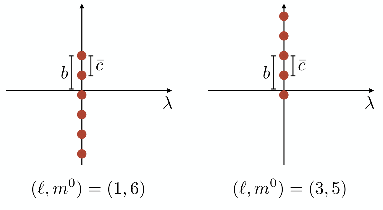
Writing for and with all symbols positive, we check the consistency of this string solution by inserting (31) into (30). We obtain, to logarithmic accuracy,
| (32) |
with again by convention. This can be solved and we obtain
| (33) |
The system of equations (32) is slightly different if or but the solution (2.3.2) for the remains identical. The solution (2.3.2) can then be used to conclude on the domain of stability of these solutions: this string solution is consistent with the Bethe equations if all the symbols are positive. Requiring this in general implies a lower bound on (from the first line of (2.3.2), that only exists if ) and an upper bound on (from the second and third lines of (2.3.2)). It can be seen that the most restrictive lower bound is obtained for by requiring that , and the most restrictive upper bound is obtained by requiring that . From that we obtain that the string state exists if
| (34) |
We summarize for clarity the possible boundary strings as a function of in the Table 1.
| Value of | Allowed Boundary Strings |
|---|---|
| , | |
| and | |
| and | |
| and | |
| and | |
| and | |
| , | and |
In the Table 1 the constraint is of course always obeyed, but not all values of in that interval are always possible, some may be missing depending on the value of (for instance is always missing for ).
Remark 2.4.
Let us emphasize that other solutions can be obtained by changing the sign of one or more rapidities inside the string state. Such a solution however correspond to the same quantum state and by restricting ourselves to states of the form (31) we have defined a family of representant of the possible states.
Physically, these states correspond to clusters of particles that are bound to the wall (‘boundary strings’) and confined around . Here we give 4 examples of wave-functions.
- •
, : . For a single boson it is clear that there will be a one body bound state only for , which is when this state becomes normalizable and exists in agreement with the table.
- •
, : . This state exists for any . Hence, the remarquable feature is that already for there can be a two-boson bound state even for , i.e. for a repulsive wall. Note that it decays as if only one particle (the second for ) is far from the wall and as if both are far from the wall (for ).
- •
, : For there is another possible value for , which is (we recall the constraint ). This two-boson bound state is more complicated that the state, and reads
(35) Note that this eigenstate exists only in the restricted range . It decays as if only one particle (the second for ) is far from the wall and as if both are far from the wall (for ). Each of these two decay rates precisely vanish at one endpoint of the stability range.
- •
, : . From the Table 1 this eigenstate always exists for and exists for for . Note that in the range of existence, the formal vanishing of the prefactor for some integer values of is compensated by the norm. It turns out that this state is the ground state for some range of parameters, as discussed below.
It can be checked that the states in Table 1 are normalizable iff the condition of existence on (2.3.2) are satisfied. Although it is clear that these states correspond to states that are bound to the wall, we do not have a full physical interpretation of them. In particular the physical interpretation of the parameter is lacking. We do not have a satisfying understanding of the remarkable fact that some states can exist even when (repulsive wall). At a very qualitative level, by examining the alternative form (16) for the Hamiltonian (see discussion there), one could argue that the ”image” interaction term produces, when two particles meet at the wall, an effective ”additional” attraction to the wall (an effective term). Finally, the examples studied above suggest some insight on the domain of stability, but which remains still very partial. The wavefunction (2.2) contains terms (many with vanishing coefficients) of the form where is given in (31) (from now on we consider infinite and set the deviations ). Consider the decay when all particles are moved to , . We note that the term where all leads to a term whose condition for decay is identical to the upper bound in (both lines of) Eq. (2.3.2). We did not find such a simple interpretation for the other condition in (2.3.2).
It is interesting to know, as a function of , how many boundary string states exist with a given string multiplicity , which we call . The formula, obtained from Table 1, is given in the Appendix A.
It is useful to introduce the center of mass of the boundary string
| (36) |
We will see that boundary strings formally share similarities with usual strings with . In particular the energy eigenvalue of a boundary string eigenstate is obtained as
| (37) | |||||
with as in (28).
2.3.3 General case: boundary and bulk strings.
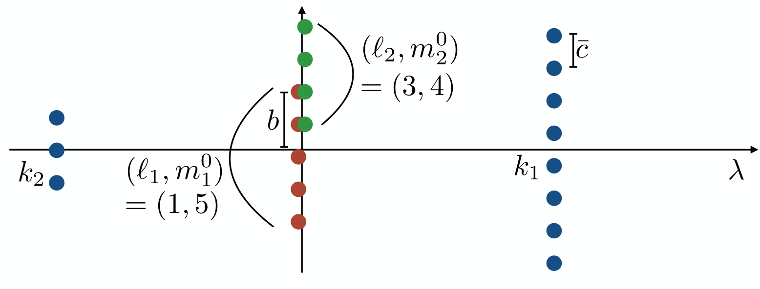
For any finite , we conjecture from the above study that a general -particles eigenstates can be obtained, in the limit, by partitioning the particles into clusters of particles. The first clusters of particles are bulk strings with multiplicities , , string momenta and rapidities inside the string given by (27) (setting terms to zero). The remaining clusters of particles are boundary strings with ‘-numbers’ and multiplicities , and rapidities inside the string as given by (31) (setting terms to zero). The fact that several boundary strings can coexist in the same state is non trivial 55 5 It leads formally to coinciding rapidities for which is forbidden for an eigenstate at finite . This restriction may not apply however in the limit, if the difference vanishes in that limit. We have not checked in details that this mechanism, known in several other cases [40, 122], occurs here, but we are led to conjecture that it does, from consistency considerations in the calculations of Section 3. The values of the different integers must now satisfy , , with (only one of the two sums can be empty) and the integers such that the condition of stability of the boundary string (2.3.2) is satisfied. The energy of such a state is with as in (28).
Remark 2.5.
We should stress that we have no proof that this set of states is complete in the sense that it provides a complete basis of the Hilbert space on which acts the LL Hamiltonian . This will be our working hypothesis in the following. Our results on the KPZ/DP problem in the next Section, which are an application of this study, are quite consistent with this hypothesis.
2.4 Norm of string states
The calculation of the norm of string states starting from the finite size formula (120) is a tedious exercice that requires a careful evaluation of many singular terms that are regularized using the string deviations , in the same way as for usual strings in the attractive Lieb-Liniger model [92]. We report the details of the derivation in Appendix D and only give here the result: given a state characterized by the set of integers and bulk strings momentas as in Sec. 2.3.3 we obtain its norm as
| (38) | |||||
where we have introduced the notations
| (39) |
Note that are even in for integer (see below for equivalent expressions where it is more apparent). We also introduced
| (40) | |||
and we recall the definition (36) of the boundary string center of mass . Note that the norm of a state scales as as a signature of the fact that the bulk strings are delocalized and almost behave as free particles. On the other hand the norm of a pure boundary string does not scale with , showing that these states are localized in space. The formula (38), presented here as a conjecture, has been checked numerically for states with a small number of particles.
In the hard wall limit studied in [76], one has and the boundary strings do not exist. The above formula (38) reproduces formula (9)-(10) of [76], correcting for the misprint there, i.e. replacing there and in all three lines of (9-10). With these corrections, the definition of the factor there equals the factor here, and the factors are the same. Note that all other definitions there, such as the wavefunction (2.2), are the same as here.
2.5 Ground state of the attractive Lieb-Liniger on the half-line
We now discuss the properties of the ground state for a system of particles as a functions of and . In the absence of states bound to the wall (), reminiscent of the usual attractive LL model on the full space, it is well known that the ground state is obtained by putting all particles in a single string state with string momenta . We recall that the energy for a string of particles with string momenta is (see (28))
| (41) |
And the ground state energy is thus in the case . In the finite case one can hope to find states with lower energy since the energy of the boundary string is with imaginary and given by (36): we recall that
| (42) |
Note that as a function of , is a parabola which reaches its maximum for . Since this value coincides with the upper bound on that is set by the condition of existence of the boundary bound state (2.3.2), we can conclude that the boundary bound state with the minimum energy is obtained by taking which indeed always exist if any boundary bound state does. The energy of this state is
| (43) |
and we can conclude that this state is the ground state whenever it exists, that is when . To summarize we have obtained that
- •
For the ground state is a state made of a single bulk string with vanishing momenta. The ground state energy is . The ground state wavefunction in the bulk (i.e. for all points far from the boundary66 6 near the boundary it takes a more complicated, -dependent, form where is the (small) momentum.) looks like the ground state of the full space problem
(44) - •
The transition occurs for . Exactly at the transition the two states are formally identical as their rapidities are the same (nondegenerate ground state) i.e. (31) and (27) coincide, , but the state should be considered as a bulk string ground state as it is delocalized in the full volume. The ground state energy is continuous across the transition. A cartoon of the transition is shown in Fig. 6.
Remark 2.6.
One can explore the possibility that the ground state is composed of several strings. For bulk strings it is well known that splitting them only leads to excited states. Let us consider the state with two boundary strings of particle content and . For each of them the same arguments as above, replacing by shows that is the best choice. We now note that
| (46) |
is always strictly positive for and in the domain . For this is always true for . For , since we have assumed that (the condition of stability for each string) it implies . Hence it is never advantageous to split a boundary string into two boundary strings and the ground state is thus composed of a single boundary string in the region as stated above.

2.6 Decomposition of the identity in terms of Lieb-Liniger eigenstates
We conclude this section by writing explicilty the decomposition of the identity that follows from our classification of states as a function of . Let us first write the formula and then comment it. On the space of symmetric functions of variables with the appropriate boundary condition (20) at the identity can be written as
| (47) |
where
- •
denotes the state with rapidites arranged in boundary and bulk strings according to the numbers and as explained before.
- •
The sum denotes the sum over the possible integers parametrizing stable boundary strings as a function of (see (1) for the domain of stability).
- •
The factorial factors avoid multiple countings of the same state.
- •
The phase space factor is standard and can be determined by studying the reduced Bethe equations satisfied by the string momenta [92]. Note two differences compared to [92] here: the quantization is and not due to the additional factor of inside the exponential on the left-hand side of the Bethe equations (24); the integral over only runs from to since states with string momenta and string momenta are identical.
Remark 2.7.
The formula for the decomposition of the identity (2.6) can be modified using the symmetries of the Bethe states. In particular can be transformed into . This will be useful in the section on the application to the directed problem in order to obtain formulas with the desired symmetries made explicit.
3 Application to the KPZ equation/directed polymer problem on the half-plane
In this section we use our study of the Lieb Liniger model on a half-line to study the continuum directed polymer/KPZ equation on a half-space as introduced in Sec. 1.2. We start by giving our result for the integer moments of the partition sum of the DP for fixed endpoints near the wall. Given these formulas, we already show that the existence, and some properties, of the transition at as the interaction parameter with the wall is varied, can be obtained from the contribution of the quantum ground state of the Lieb Liniger model. These results confirm earlier results by Kardar [74] and put them on a firmer basis. We then use our expressions for the integer moments (which are valid at all times) to obtain the exact statistics of the KPZ height-field/directed polymer free-energy, at large time/large polymer length . We show that the fluctuations of the appropriately rescaled variable changes from GSE-TW type fluctuations () of width to Gaussian fluctuations () of width , with at the transition point GOE-TW type fluctuations of width . We recall that, here and throughout this section, the DP model defined in Sec. 1.2 is associated, as in Sec. 1.3, to the LL model studied in the previous section where the parameters has been set to by a choice of units.
3.1 Moments of the DP partition sum for fixed endpoints near the wall
3.1.1 Starting formula for the moments
From now on we focus on the partition sum of the directed polymer introduced in Sec. 1.2 for fixed endpoints at the wall (droplet initial conditions in the KPZ framework). We use in the following as a shorthand, . We start from the formula (15) giving the moments in terms of the eigenstates of the LL model and now make it explicit using the results of the previous section. Using , and decomposing an arbitrary eigenstate in terms of boundary and bulk strings as in Sec. 2.3.3, it is a simple exercice to see that we can write
| (48) |
where we have introduced
| (49) |
and used that for integer . Note that is explicitly even in and that for integer the product is an even polynomial in . Combining this with the decomposition of the identity (2.6) and the formula for the norm of string states (38) we get
| (50) |
3.1.2 Symmetrization
We now obtain an equivalent but more symmetric formula. We introduce for simplicity the following function
| (51) | |||
that enters into (3.1.1). We recall the definitions (2.4) of the functions and and (49) of . It is easily checked that is even in , as are the other factors that contain in (3.1.1), i.e. . The integration on can be extended to an integration on , adding an addition factor in the measure. To make the contribution of boundary strings more symmetric, we will use the following notational trick. For a function which has a simple pole at we write
| (52) |
which we will apply to . The factor will contain all the other factors in (3.1.1). For generic (non integer) values of they do not have poles at hence they can be entered into the residue . Even then, the integral in (52) is formal since . Note that since the product is a polynomial (see (54) below), hence we can indifferently apply the residue operation to or to .
This allows to introduce (fictitious) integrals over boundary string momentas . Using finally the (anti-)symmetry of the residue, , we rewrite (3.1.1) as
| (53) |
where we recall that the integral over with the delta function terms simply and only means to take the corresponding residue in the factor .
Eq. (3.1.2) is our main final exact result for the moments of the DP partition sum, equivalently the exponential moments of the KPZ height at the boundary, , for droplet initial conditions. We stress that it is valid at all times and for any .
Remark 3.1.
In the limit , the factor becomes unity and
| (54) | |||
for integer . There are no boundary strings and the formula (3.1.2) identifies with Eq. (11) in [76] (with the same factor as here, note the misprint in (10) there should be , see discussion at the end of section 2.4). Note that in the l.h.s. of Eq. (11) of [76] should be identified as , which has a finite limit for , also equal to (Eq. (8) there).
3.2 Ground state physics and KPZ height function
The ground state phase transition discussed in the Lieb-Liniger context in Section 2.5 allows to obtain some properties of the phase transition in the directed polymer context. Here the interesting quantity is the directed polymer quenched free-energy in our units. We will focus on the KPZ height field , which is equivalent, and simply equal to minus the free energy of the DP, . At large time, both grow linearly plus fluctuations
| (55) |
with is a random variable of order , and we denote by the KPZ growth speed. Here is the growth exponent, to be determined below. In the DP context, is also called , the free energy fluctuation exponent.
The average free-energy per-unit length can be obtained from the replica trick in the limit as
| (56) |
Inverting the limit on and , one approximates by (i.e. retaining only the ground state contribution for large). The explicit expression for the ground state energy of the LL model in a half-space was given in Section 2.5. Performing its analytical continuation to real in the naive way we can expand around and we obtain two cases (see Figure 6).
- •
For (recall that in our present unit) the ground state is for sufficiently close to obtained by putting all particles in a bulk string with zero momentum and we obtain, expanding in
(57) which is the standard value for the full space continuum KPZ equation77 7 We recall that this negative value comes from the Ito prescription in the continuum SHE with white noise. If e.g. a space-time cutoff on the noise is used instead, an additional, non universal positive constant is added to (in both phases, and at most smoothly varying with , so it does not affect the universality of the transition studied here)..
- •
For , the ground state is always obtained as a boundary string and we obtain
(58) hence the free energy per unit length, , is lower in this phase.
We can therefore conclude that the DP exhibits a phase transition at . This is a binding transition in presence of disorder, from a bulk phase where the polymer rarely comes back near the wall, to a bound phase for , where the polymer spends a macroscopic fraction of its length near the wall. We thus confirm here the arguments of Kardar [74], via a detailed analysis of the boundary strings (only the state was considered there) 88 8 In our units, the correspondence holds setting the parameters there , , and .. Note that at this stage we have not specified the initial conditions (for KPZ) i.e. the endpoints conditions for the polymer.
Remark 3.3.
Note that this most naive replica trick correctly predicts the extensive part of the free energy, i.e. predicts via the linear term in in . One could attempt to expand in powers of near to predict fluctuations. In the full space problem, it is well known that it fails, as the and (or analytical continuation in ) do not commute since the limit has already been taken [121]. Hence we can anticipate that here in the unbound phase it also fails. This will be discussed again below.
3.3 Rescaled free-energy, KPZ height and definition of the generating function
In order to study the statistics of the free-energy of the DP at large time we decompose (for arbitrary time)
| (59) |
with given in the precedent section and is the centered and scaled KPZ height, a random variable. In our units (which amount to set in the LL model) we thus have
| (60) |
As written in (59) the probability distribution function (PDF) of (minus) the rescaled height function depends on , but here we will show that, choosing the growth exponent as
| (61) |
then is an random variable whose PDF in the infinite time limit will be computed below. We will show that for , is distributed according to the GSE-TW distribution, for , is distributed according to the GOE-TW distribution and for , is distributed according to a Gaussian distribution.
To compute the distribution of we first define the following generating function:
| (62) |
Let us introduce a unit Gumbel random variable , statistically independent from , with cumulative distribution function (CDF), . Then from (62)
| (63) |
which is an exact formula for all . In the large time limit it simplifies as
| (64) |
i.e. the CDF of the centered and scaled KPZ height at infinite time coincides with the large time limit of the generating function. Our strategy is thus as follows: we first compute (62) using the expression for (3.1.2) and show that can be written as a Fredholm Pfaffian at all time . We will then perform an asymptotic analysis of these formulas at large time in the different phases, sheding light on the phase transition at the level of the fluctuations of . Anticipating the calculations, we obtain
- •
- •
Critical boundary regime: . In the limit one has
(67) with the GOE kernel expressed as
(68) and the CDF of the GOE-TW distribution.
- •
Attractive boundary regime: . In the limit one has
(69) with a Gaussian random variable with mean and variance .
3.4 From the moments to the generating function as a Fredholm pfaffian
Here we will follow a route quite similar to [76], although more involved because of the presence of boundary strings. We first use the Schuhr Pfaffian identity (see Appendix E for the definition of the Pfaffian and its properties)
| (70) |
with and for and and for . Using these identities, the definition of the generating function (62) and the formula for the moments (3.1.2) we obtain the following expression for the generating function
| (71) |
Now we use the following identity
| (72) |
and standard properties of the pfaffian to move the integrals outside the pfaffian (see Appendix). This gives
| (73) |
Note that this has the following structure:
| (74) |
where we have introduced two antisymmetric functions given by
| (75) |
where we recall that
| (76) |
and
| (77) |
We can now ”undo” our notational trick and obtain the following definition of the antisymmetric function as
| (78) |
where we recall that and (for integer )
| (79) |
Remark 3.4.
Note that exactly at the transition for the -bound state, i.e. when (see discussion below Eq. (44)) there is a removable singularity at in the integral for of the type . Correspondingly there is no bound state exactly at the transition.
Using the symmetries of the integrand in (3.4) it can be seen that we can finally rewrite as
| (80) |
Here we have used that for an arbitrary antisymmetric function and integer
| (81) |
as can be easily checked using the definition of a Pfaffian, being the number of pairings of objects. Using this identity with and , the identity between (3.4) and (80) is easily checked term by term at fixed (notice that the terms with odd in (80) vanish). We also used that the product of two Pfaffians can be written as the Pfaffian of a block diagonal matrix. Finally, as is shown in the Appendix E.2 using properties of Fredholm Pfaffians, we obtain our main exact result for the generating function, valid at arbitrary time and boundary parameter
| (82) |
with
| (83) |
and the projector on : . We recall that the generating function was defined in (62), and that the antisymmetric functions and are defined in (75),(78). Above and throughout this work denotes the Fredholm determinant associated to a kernel which is a linear operator acting on (a subset of) .
It is useful to note the following property. Suppose that the kernel is associated to , i.e. . Denote with . Then the kernel associated to is with . Since it is obtained from by a similarity transformation one has
| (84) |
Hence, the generating function is unchanged by any scale transformation on the arguments of . We will note below the kernel with scaled arguments (and respectively and their components).
3.5 Matching with the result of Ref. [82] for
In the previous section we have obtained the generating function in Eqs. (82), (83) in terms of a kernel involving the antisymmetric functions and defined in terms of formal sums over integers in (75),(78). On the other hand in Ref. [82] we have obtained
| (85) |
in terms of an antisymmetric function expressed as
| (86) | ||||
with . This is obtained from (86-87) in Ref. [82] using the identity
| (87) |
with .
We now show that for the two results match in the following sense. If we rewrite as a sum over residues in and move the contour in appropriately we can rewrite as a formal sum over integer as
| (88) |
In order to show this let us close the contour on in (86) on the right, since . The poles in are at (we denote them as poles of type I), and at (we denote as poles of type II).
We can first show that the poles of type I have a vanishing contribution. Indeed the residues of these poles give as a sum with the following structure
| (89) |
Closing the contour on on the right, we see that poles of the Gamma function on the numerator at give a residue proportional to and therefore vanish. The poles of the the sine on the denominator are canceled by the .
Thus we only need to consider poles of type II. For these, using we obtain
| (90) |
One then sets with .
In order to show equivalence to the kernel we now need to shift back to the real axis. To do that one notices that in the band the only poles arise from the Gamma functions in the numerator and are located at and . Hence we must have the following inequalities
| (92) |
One can check that the conditions for these poles to have non-zero residue (from the Gamma functions in the denominator) are which is automatically satisfied if (92) is obeyed.
Remark 3.5.
Note however that when is a positive integer, the residue associated to and the residue associated to cancel one another. Hence we can make the inequality strict.
The shift of the contour thus gives
| (93) | |||
| (94) |
where is the sum over the residues, see below, and is defined in (76) . We can already see, comparing with (75) and using that for , that
| (95) |
From the definition of in (3.4),(78) as residues of , we see that in order to show that
| (96) |
one only needs to show that the allowed values of , and correspond exactly to the allowed values of which label the bound states.
We now explain the correspondence between these poles and the boundary bound states which contribute to . The index is the same in both cases, and we set . The residues at indicate the poles of rather than so for simplicity we can reduce to the study of the poles at . From the constraints (92) plus Remark 3.5 (see also Remark 3.4) the integer must satisfy
| (97) |
This is clearly equivalent to the bound state structure presented in Table 1 (see also (2.3.2)). This completes the identification (88) for the unbound phase . Note that the factor of in the variables is immaterial in the evaluation of the Fredholm determinant as can be seen using the similarity transformation (84) with . Hence we have shown that the main result (82), (83) is formally equivalent (at all time ) to the result of Ref. [82] for .
3.6 Discussion on the Mellin-Barnes summation formula for
For other RBA solutions of the KPZ equation, in order to evaluate the formal sums over integers (arising from the summation over the eigenstates of the LL Hamiltonian) one uses the so-called Mellin-Barnes (MB) trick, which allows to rewrite the sum over the string lengths as an integration over a contour in the complex plane
| (98) |
where with . However one fundamental assumption of the equality above is that the function has no poles on the half-plane. The kernel instead contains the function
| (99) |
It is easy to see that this functions has poles as function of at positions
| (100) |
with a positive integer. Hence when performing MB one must take into account these extra poles. As we have shown in the previous section, these extra poles correspond exactly to the bound state contributions carried by the kernel . Backtracking the steps performed in the previous section allows to perform the correct MB summation for . Performing the MB summation for is left for a future study.
3.7 Large time limit: unbound phase,
In a previous section we have obtained the generating function at all times in Eqs. (82), (83) in terms of a kernel . Then we have shown that for this kernel is identical, up to a similarity transformation that leaves the Fredholm determinant unchanged, to the kernel of Ref. [82], . As it was shown in [82] the generating function obtained from the kernel defined in (85), (86), converges in the large time limit to the TW-GSE distribution for and to the TW-GOE distribution at . Setting
| (101) |
and taking the large time limit at fixed , allows to explore the critical crossover region by varying from to . The transition kernel is obtained by setting for and rescaling in (86) the variables as
| (102) | |||
| (103) | |||
| (104) |
Taking the large time limit of the kernel one obtains indeed
| (105) | ||||
where .
- •
In the limit one recovers the standard GSE kernel, therefore giving
(106) with .
- •
The other limit, , requires particular care. First the integration contour for and need to be shifted to the right of . Then the limit can be taken, as shown in [82], giving the scalar form of the GOE kernel
(107) with .
3.8 Large time limit: bound phase
Let us discuss now the bound phase, . The formula Eqs. (82), (83) for the generating function at all times in terms of the kernel remains correct. Unfortunately, the summation over all eigenstates (i.e. all integers ) remains at present our of reach. However, inside the bound phase, it reasonable to expect that the large time limit is given by the contribution of the bound state to the wall formed of a single boundary string with . As we show below it predicts a Gaussian distribution for the fluctuations of the free energy of the directed polymer (i.e. of the KPZ height) at the origin at large time. Such a distribution is expected from universality and the results on the discrete models, e.g. [64].
A physical argument can be given. For this state is the ground state of the LL model for any . The reason why restricting to the ground state does not reproduced the full physics in the case is because the limit is taken before the limit. In the quantum language the phase is gapless and the full spectrum of excitations contributes to the fluctuations of (for examples pure bulk string states with and and a small string momenta have an energy that is arbitrarily close to the ground state). On the other hand when the system is gapped. The effect of taking does not change the problem, since the polymer remains bound to the wall and its typical wandering away from it is . By contrast, in the phase it explores distances to the wall of order .
We thus start back from the initial expression of the generating function (62), with , from (58), and using (3.1.2) for and retaining only the contribution from the ground state , which, as was discussed in section 2.5 is a boundary string , , and . We obtain using (79)
We use the Gaussian decoupling
| (108) |
and a MB formula similar to (98) for the sum over
| (109) |
where with . To obtain the large time limit, the proper rescaling for the variable is not given by but by . We thus write , in which case the cubic term disappears at large time, leading to
| (110) |
We thus obtain a Gaussian distribution for the rescaled height
| (111) |
showing that is a Gaussian random variable of variance .
4 Conclusions and future directions
In this work we have conducted a systematic analysis of the attractive Lieb-Liniger model on the half-line. In the closely related XXZ spin chain problem it corresponds to open diagonal boundary conditions.
In particular we have characterized its spectrum of boundary bound states as a function of the particle number and of the interaction with the boundary. We expect that these results may be of interest in the context of quantum quenches in restricted geometries and non-linear Schrodinger systems.
These results have been used to obtain predictions via the replica Bethe ansatz for the fluctuations of the KPZ equation next to a wall. The height of the KPZ function, which also maps to the free energy of the directed polymer in presence of disorder on the half space, displays a phase transition at the critical value of the interaction with the wall. We have obtained the three types of statistics that govern the fluctuations in the different regimes: attractive boundary, critical boundary and unbounded growth, described respectively by the Gaussian, GOE-TW and GSE-TW distributions.
Moreover we quantify the KPZ front velocity. The present results complement the
ones obtained in Ref. [82] and are in agreement with results previously obtained in
a number of works on discrete models, thereby consistent with the universality of the transition.
Although the exact formula for the integer moments of the partition sum of the directed polymer
have been obtained here for all and time , extracting the PDF (i.e. the generating function at all time) has been possible only in the unbound phase and at the transition.
One of the remaining open questions is to obtain a complete solution for the bound phase at
arbitrary time, e.g. by developing a specific Mellin-Barnes method. Obtaining the
GOE-Gaussian crossover kernel in the large time limit (for ) for the
KPZ equation would be of great interest and could be compared with
the results of Ref. [68] for the discrete model.
By duality, the case amounts to study a Brownian IC with a
positive drift, which is also of interest: this would result in a better understanding of the summation method which could then probably
be extended to the full space case. In addition, results for endpoints
away from the wall would also be desirable.
Finally, the same type of phase transition is expected to take place in the quantum regime, in particular in cold atomic systems which are governed by the attractive Lieb-Liniger Hamiltonian. It will be fascinating to experimentally observe a similar localization transition around a point-like defect, for example induced by a local laser field, simply by tuning its intensity.
Acknowledgments
We are grateful to Guillaume Barraquand for very useful remarks and pointing out references. We also thank A. Bufetov, I. Corwin, A. Borodin, K. Takeuchi, N. Zygouras for discussions. This work is supported in part by LabEX ENS-ICFP:ANR-10-LABX-0010/ANR-10-IDEX-0001-02 PSL* and Research Foundation Flanders (JDN and TT), ANR grant ANR-17-CE30-0027-01 RaMaTraF (PLD and AK), ERC under Consolidator grant (AK) number 771536 (NEMO) and the National Science Foundation under Grant No. NSF PHY11-25915 during the randomKPZ16 program at the KITP.
Appendix A Number of boundary strings
The number of boundary strings for a fixed value of is equal to the number of values of possible for a given . From the Table 1 we find, denoting the integer part of
- •
For , we have, for
(112) and for .
- •
For , and not an integer99 9 From Table 1, we have and for , is one plus the number of integers in the interval , we have for , then for
(113) with for , for , and finally for .
Appendix B Lieb-Liniger model on the half line as the scaling limit of an open XXZ spin- chain with longitudinal fields at the boundaries
We consider the XXZ spin 1/2 chain with open boundary conditions. In particular we focus on the case where at the two boundaries two longitudinal fields are applied, so-called diagonal boundary conditions. The Hamiltonian is given by
| (114) |
with and with the longitudinal fields parametrised as . Its diagonalization can be performed by a modified version of the algebraic Bethe Ansatz proposed by Sklyanin in [111] and some properties of its correlation functions are known [112, 113]. The resulting Bethe equations reads as
| (115) |
The Lieb-Liniger model on the half line is given by the model (114) with the following scaling limit [123]
| (116) | ||||
| (117) | ||||
| (118) | ||||
| (119) |
In this limit the Bethe equations (B) become the Bethe equations for the Lieb-Liniger model on the half-line with boundaries parametrized by and and with attractive coupling (24)
Appendix C Norms of the string states
We detail in this appendix the derivation of the norm of the string states (38) starting from the finite size norm formula (120). The non-trivial aspect of this calculation amounts in principle in evaluating the determinant in (120). The symplifying feature that allows an exact formula is that both the prefactor and the determinantal part in (120) are singular for string states with rapidites of the form (31) (boundary strings) or (27) (bulk strings): the prefactor tends to zero with the string deviations while the determinant diverges. This means that in the large limit it is sufficient to evaluate the most singular term of the determinant which, combined with the trivial prefactor, gives the exact result. For a state of particles made of bulk strings and boudnary strings, it can be seen that this most singular term factorizes among the different strings (divergent terms inside the determinant only appear within blocks inside a string). For this reason we evaluate here the norm for the special cases of a state made of (i) a single bulk string; (ii) a single boundary string. The final formula (38) then easily follows using the factorization property.
C.1 Norm of a propagating string
The above eigenfunctions are not normalized. We conjecture, that their norm is a generalization of the full space Gaudin determinant [104], given by
| (120) | |||||
where
| (121) |
and
| (122) |
We comment on the rationale behind this conjecture in Appendix D. We note that this formula agrees with the conjecture already presented in [107] and on the scaling limit (see Appendix B) of the norm of the open XXZ eigenstates [112] (formula 4.26 in that paper).
We start here with the case of a single bulk string with rapidities in the with and . We reintroduce explicitly the string deviations as follows: and note . We have introduced a factor in front of the string deviations compared to (27) to make the parallel with [92] transparent. Two terms appearing in the prefactor of the norm formula (120) are non singular:
Note that in the text we use the notation . The singular term is evaluated, to leading order in the string deviation, as
| (123) |
This is cancelled by a divergence coming from the Gaudin determinant:
| (124) |
This follows by proceeding exactly as in Appendix B of [92] to which we refer for more details and here we recall the main idea: divergent terms inside the determinant are on the three main diagonals of the Gaudin matrix and are those of the form with . . All these terms can be put onto the diagonal by applying the following transformation on the matrix: first add the first column to the second one then the first row to the second row (tranformations that leave the determinant unchanged). Then the term only appears inside the entry of the matrix. Now add the second column to the third one and the second row to the third one. Then the term only appears inside the entry of the matrix. Proceed recursively. Once all terms are on the diagonal, the determinant is evaluated by taking them. The entry of the matrix is also automatically taken and is to leading order equal to in the large limit. This leads to the above result. Taking all terms into account, the norm of the string state is evaluated as
| (125) |
which can be seen to be in agreement with (38), i.e. for such a single bulk string state with and , one has (there are no inter-string factors , see below).
C.2 General case
The general case of a state made of bulk strings and boundary strings easily follows from the factorization property of diverging terms inside the determinant. The careful evaluation of the prefactor of (120) for such a state leads to the inter-string factors noted as in (2.4). Note that for boundary strings, we have noticed that the conjectured formula misses a factor per each boundary string, which we have corrected for the formula we use, eq. (38).
Appendix D Gaudin determinant for the norm of Bethe states on the half-line
The logic behind the conjecture (120) follows from the study of other models that are integrable by coordinate Bethe ansatz: inside the determinant is inserted the matrix that is the derivative of the logarithm of the Bethe equations [124]:
| (126) |
Notice that this formula was already conjectured in [107]. The prefactor in front of the determinant is then guessed by expanding formally the norm as a double sum over permutations for real rapidities (corresponding to a state with , i.e. with one-strings (i.e. ”particles”) in the large limit) as, schematically, taking the modulus square of (2.2)
and to leading order in , the only terms that survive are those with and . This leads to
with corrections of order . This expression is indeed the leading order in obtained from the computation of the Gaudin formula (120) with the prefactor as above.
Appendix E Pfaffians, Fredholm Pfaffians and Fredholm determinants
Pfaffians
Let us first recall the definition of the Pfaffian of an antisymmetric matrix of size
| (128) |
with . Since the determinant of an antisymmetric matrix of odd size is zero, the Pfaffian can also be set to zero. For it is , for it is , and so on, the number of terms in the sum is , the number of pairings of objects. In the text we use the Schur Pfaffian identity
| (129) |
E.1 Fredholm Pfaffians and Fredholm determinants
We here shortly review how Fredholm determinants and Pfaffians are defined. Given a kernel and a domain we define a trace-class operator satisfying
| (130) |
Its Fredholm determinant is defined as the infinite convergent sum
| (131) |
where we introduced the operator as a projector on the domain and the identity operator . Following Ref. [125] we can see the Fredholm determinant as a discretization of the domain in points with associated weights such that given any integrable function on we have
| (132) |
then the Fredholm determinant (131) is the limit of the determinant of the matrix
| (133) |
A generalization of the Fredholm determinant is given by the Fredholm Pfaffian defined for antisymmetric matrices. Given a two-by-two matrix kernel
| (134) |
then we define its Fredholm Pfaffian on the domain as
| Pf | (135) | |||
| (136) | ||||
| (137) |
where we introduced the two-by-two kernel
| (138) |
The connection between Fredholm Pfaffian and Fredholm determinant is given by
| (139) |
E.2 Derivation of the formula (82), (83) in the text
The expression (80) for the generating function can be rewritten as a Fredholm pfaffian:
with and both antisymmetric kernels. Here we assume implicitly that all integrations are on , i.e. we do not write the projectors explicitly. The above form has similarities to the one obtained for the flat KPZ problem in Section 6.5 of Ref. [40]. The main difference is that here there is no off-diagonal part , which makes the problem simpler (as discussed there, there are two definitions of the ordering in a FP, which accounts for the minus sign.). We now follow the same steps as in Section 6.5 of Ref. [40], i.e. the square of a FP is a Fredholm determinant:
where we have defined:
| (148) | |||
| (149) |
It is shown in Section 6.5 of Ref. [40] that:
| (150) |
Appendix F Analytical continuations of the norm for arbitrary complex and
We recall that where, for integer , using , is a polynomial which can be rewritten in several equivalent ways
| (151) | |||
| (152) | |||
each of them leads to an analytical continuation by replacing . For instance the last two give
| (153) | |||
| (154) |
Note that the second has a term compared to the first. These factors are important since they allow to use the MB formula. Similarly,
| (155) |
has several analytical continuations. The first one is
| (156) |
But, for instance there are two others
| (157) |
and
Note that for and
| (159) |
We will therefore use the following analytical continuation for the function
| (160) |
It can be checked that the first part of this formula reproduces the definition of (51) for any . This part is also even in for any but not for . In order to keep the symmetry of the integrand for any we have thus symmetrized the analytical continuation.
References
References
- [1] M. Hairer, Solving the KPZ equation, Ann. Math. 178, 559, (2013).
- [2] J. Baik, E. M. Rains, Limiting distributions for a polynuclear growth model with external sources, J. Stat. Phys. 100 523–541, (2000).
- [3] M. Prähofer and H. Spohn. Universal distributions for growth processes in 1+ 1 dimensions and random matrices. Physical Review Letters, 84(21):4882, (2000). Scale invariance of the PNG droplet and the Airy process, J. Stat. Phys. 108 1071–1106, (2002).
- [4] P. L. Ferrari, Polynuclear growth on a flat substrate and edge scaling of GOE eigenvalues, Comm. Math. Phys. 252, 77 (2004).
- [5] P. L. Ferrari and H. Spohn, Scaling Limit for the Space-Time Covariance of the Stationary Totally Asymmetric Simple Exclusion Process, Comm. Math. Phys. 265 1 (2006)
- [6] P.L. Ferrari The universal Airy1 and Airy2 processes in the Totally Asymmetric Simple Exclusion Process, arXiv:0701021
- [7] T. Sasamoto. Spatial correlations of the 1D KPZ surface on a flat substrate, J. Phys. A 38.33 (2005).
- [8] S. Prolhac, Finite-time fluctuations for the totally asymmetric exclusion process, Phys. Rev. Lett. 116, 090601, (2016). Current fluctuations and large deviations for periodic TASEP on the relaxation scale, J. Stat. Mech. (2015).
- [9] C.A. Tracy and H. Widom, A Fredholm Determinant Representation in ASEP, Journal of Statistical Physics, 132, 291-300, (2008).
- [10] C.A. Tracy and H. Widom, Asymptotics in ASEP with Step Initial Condition, Communications in Mathematical Physics, 290, 129-154, (2009).
- [11] A.M. Povolotsky, On the integrability of zero-range chipping models with factorized steady states, J. Phys. A, 46:465205, (2013).
- [12] A. Borodin and I. Corwin, Macdonald processes, Prob. Theor. Rel. Fields 158 (2014), no. 1-2, 225–400, arXiv:1111.4408.
- [13] I. Corwin, Macdonald processes, quantum integrable systems and the Kardar-Parisi-Zhang universality class, Proceedings of the ICM, arXiv:1403.6877.
- [14] K. Johansson, Shape fluctuations and random matrices. Commun. Math. Phys. 209, 437 (2000).
- [15] T. Seppäläinen, Scaling for a one-dimensional directed polymer with boundary conditions, Ann. Probab., 40 :19-73, (2012), arXiv:0911.2446.
- [16] T. Thiery et P. Le Doussal, Log-gamma directed polymer with fixed endpoints via the replica Bethe Ansatz, Journal of Statistical Mechanics: Theory and Experiment 10, 10018, (2014).
- [17] I. Corwin, N. O’Connell, T. Seppäläinen, and N. Zygouras, Tropical Combinatorics and Whittaker functions arXiv:1110.3489. Duke Math. J., 163, 3, 513-563, (2014).
- [18] A. Borodin, I. Corwin, et D. Remenik, Log-gamma polymer free energy fluctuations via a fredholm determinant identity. Communications in Mathematical Physics 324, 215–232 , (2013).
- [19] I. Corwin, T. Seppäläinen, et H. Shen, The strict-weak lattice polymer, Journal of Statistical Physics 160, 1027–1053,, (2015).
- [20] N. O’Connell, J. Ortmann, Tracy-Widom asymptotics for a random polymer model with gamma-distributed weights, Electron. J. Probab., 20, 25, 1-18 (2015), arXiv:1408.5326.
- [21] T T. Thiery et P. Le Doussal, On integrable directed polymer models on the square lattice, Journal of Physics A Mathematical General 48, 465001 (2015).
- [22] T. Thiery. Stationary measures for two dual families of finite and zero temperature models of directed polymers on the square lattice. Journal of Statistical Physics, 165(1):44–85, (2016).
- [23] N. O’Connell. Directed polymers and the quantum toda lattice. The Annals of Probability, 40(2):437–458, (2012).
- [24] Auffinger, A., Baik, J., Corwin, I. Universality for directed polymers in thin rectangles. arXiv:1204.4445, (2012)
- [25] N. O’Connell and M. Yor. Brownian analogues of Burke’s theorem. Stochastic Processes and their Applications, 96(2):285 – 304, (2001).
- [26] G. Barraquand and I. Corwin. Random-walk in beta-distributed random environment. Probab. Theo. Rel. Fields 167, 1057 (2017).
- [27] P. Le Doussal, T. Thiery, Diffusion in time-dependent random media and the Kardar-Parisi-Zhang equation, Phys. Rev. E 96, 010102, arXiv:1705.05159, (2017)
- [28] J. Baik, P. Deift, K. Johansson, On the distribution of the length of the longest increasing subsequence of random permutations, J. Am. Math. Soc. 12 1119–1178, (1999).
- [29] M. Kulkarni and A. Lamacraft, From GPE to KPZ: finite temperature dynamical structure factor of the 1D Bose gas, Phys. Rev. A 88, 021603(R), arXiv:1201.6363, (2012).
- [30] E. Altman, L. M. Sieberer, L. Chen, S. Diehl, and J. Toner, Two-Dimensional Superfluidity of Exciton Polaritons Requires Strong Anisotropy, Phys. Rev. X 5, 011017, (2015).
- [31] L . He, L. M. Sieberer, E. Altman and S. Diehl, Scaling properties of one-dimensional driven-dissipative condensates Phys. Rev. B 92, 155307 (2015).
- [32] M. Kardar, G. Parisi and Y-C. Zhang, Dynamic Scaling of Growing Interfaces, Physical Review Letters 56, 889, (1986).
- [33] D. A. Huse, C. L. Henley, D. S. Fisher, Physical Review Letters 55, 2924, (1985); T. Halpin-Healy, Y-C. Zhang, Kinetic roughening phenomena, stochastic growth, directed polymers and all that. Phys. Rep. 254, 215, (1995). M. Kardar and Y-C. Zhang, Phys. Rev. Lett. 58 2087 (1987)
- [34] P. Calabrese, P. Le Doussal, A. Rosso, Free-energy distribution of the directed polymer at high temperature, Europhys. Lett. 90, 20002, (2010).
- [35] V. Dotsenko, Bethe ansatz derivation of the Tracy-Widom distribution for one-dimensional directed polymers EPL 90, 20003 (2010); Replica Bethe ansatz derivation of the Tracy–Widom distribution of the free energy fluctuations in one-dimensional directed polymers, J. Stat. Mech. P07010, (2010); V. Dotsenko and B. Klumov, Bethe ansatz solution for one-dimensional directed polymers in random media J. Stat. Mech. P03022, (2010).
- [36] T. Sasamoto, H. Spohn, One-dimensional Kardar-Parisi-Zhang equation: an exact solution and its universality, Physical Review Letters 104, 230602, (2010). T. Sasamoto and H. Spohn, Exact height distributions for the KPZ equation with narrow wedge initial condition, Nucl. Phys. B 834 523 (2010), arXiv:1002.1879 ; T. Sasamoto and H. Spohn,The crossover regime for the weakly asymmetric simple exclusion process J. Stat. Phys. 140 209 (2010), arXiv:1002.1873.
- [37] G. Amir, I. Corwin, J. Quastel, Probability distribution of the free energy of the continuum directed random polymer in 1 + 1 dimensions, Comm. Pure and Appl. Math. 64, 466, (2011).
- [38] P. Calabrese, M. Kormos and P. Le Doussal, From the sine-Gordon field theory to the Kardar-Parisi-Zhang growth equation, arXiv:1405.2582, EPL 107 10011, (2014).
- [39] P. Calabrese, P. Le Doussal, Exact solution for the Kardar-Parisi-Zhang equation with flat initial conditions, Physical Review Letters 106, 250603, (2011);
- [40] P. Calabrese, P. Le Doussal, The KPZ equation with flat initial condition and the directed polymer with one free end, J. Stat. Mech. P06001, (2012).
- [41] P. Le Doussal, Crossover from droplet to flat initial conditions in the KPZ equation from the replica Bethe ansatz arXiv:1401.1081, J. Stat. Mech. P04018, (2014).
- [42] A. De Luca and P. Le Doussal, Crossing probability for directed polymers in random media: exact tail of the distribution, Phys. Rev. E 93, 032118, arXiv:1511.05387, (2016)
- [43] V. Dotsenko, Replica Bethe ansatz derivation of the GOE Tracy-Widom distribution in one-dimensional directed polymers with free boundary conditions J. Stat. Mech. P11014, (2012)
- [44] J. Ortmann, J. Quastel and D. Remenik, Exact formulas for random growth with half-flat initial data Ann. Appl. Probab. 26 507 (2016)
- [45] T. Imamura, T. Sasamoto, Exact solution for the stationary Kardar-Parisi-Zhang equation, Physical Review Letters 108, 190603, (2012). Stationary correlations for the 1D KPZ equation, J. Stat. Phys. 150, 908-939 , (2013).
- [46] A. Borodin, I. Corwin, P. L. Ferrari. B. Veto, Height fluctuations for the stationary KPZ equation, Math. Phys. Anal. Geom. 18, 20, (2015).
- [47] P. L. Ferrari and H. Spohn, Scaling limit for the space-time covariance of the stationary totally asymmetric simple exclusion process. Comm. Math. Phys. 265 1 (2006), arXiv:math-ph/0504041.
- [48] I. Corwin, Z. Liu, and D. Wang, Fluctuations of TASEP and LPP with general initial data Ann. Appl. Probab. 26 2030 (2016), arXiv:1412.5087.
- [49] J. Baik, P. L. Ferrari, and S. Péché. Limit process of stationary TASEP near the characteristic line. Comm. Pure Appl. Math. 63 1017 (2010), arXiv:0907.0226.
- [50] I. Corwin, J. Quastel, et D. Remenik, Renormalization fixed point of the KPZ universality class, J Stat Phys 160: 815, (2015).
- [51] M. Kardar, Replica Bethe ansatz studies of two-dimensional interfaces with quenched random impurities. Nucl. Phys. B 290, 582, (1987).
- [52] C. A. Tracy, H. Widom, Level-spacing distributions and the Airy kernel, Commun. Math. Phys. 159, 151, (1994).
- [53] S. Prolhac and H. Spohn, The One-dimensional KPZ Equation and the Airy Process, J. Stat. Mech. P03020 (2011), arXiv:1101.4622.
- [54] V. Dotsenko, Two-point free energy distribution function in (1+1) directed polymers, J. Phys. A. 46 355001 (2013), arXiv:1304.6571.
- [55] T. Imamura, T. Sasamoto, H. Spohn, On the equal time two-point distribution of the one-dimensional KPZ equation by replica, J. Phys. A: Math. Theor. 46 355002, arXiv:1305.1217.
- [56] J. De Nardis, P. Le Doussal, K. A. Takeuchi, Memory and universality in interface growth, Phys. Rev. Lett. 118, 125701 (2017), arXiv:1611.04756.
- [57] J. De Nardis, P. Le Doussal, Tail of the two-time height distribution for KPZ growth in one dimension J. Stat. Mech., 053212 (2017), arXiv:1612.08695.
- [58] P. Le Doussal, Maximum of an Airy process plus Brownian motion and memory in KPZ growth, Phys. Rev. E 96, 060101 (2017), arXiv:1709.06264.
- [59] K. A. Takeuchi, M. Sano, Universal fluctuations of growing interfaces: Evidence in turbulent liquid crystals, Physical Review Letters 104 230601, (2010). K. A. Takeuchi, M. Sano, T. Sasamoto, H. Spohn, Growing interfaces uncover universal fluctuations behind scale invariance, Scientific Reports 1 34, (2011).
- [60] K. A. Takeuchi, M. Sano, Evidence for geometry-dependent universal fluctuations of the Kardar-Parisi-Zhang interfaces in liquid-crystal turbulence, J. Stat. Phys. 147 853–890, (2012).
- [61] K. A. Takeuchi, Crossover from growing to stationary interfaces in the Kardar-Parisi-Zhang class, Physical Review Letters 110 210604, (2013).
- [62] T. Halpin-Healy, K. A. Takeuchi, A KPZ cocktail-shaken, not stirred: Toasting 30 years of kinetically roughened surfaces J. Stat. Phys. 160, 794 , (2015).
- [63] I. Ito, K. A. Takeuchi, When fast and slow interfaces grow together: connection to the half-space problem of the Kardar-Parisi-Zhang class, arXiv:1802.10284, Phys. Rev. E 97, 040103 (2018).
- [64] J. Baik, E. M. Rains, Symmetrized random permutations , arXiv:math/9910019, (1999).
- [65] C. A. Tracy and H. Widom, On orthogonal and symplectic matrix ensembles Commun. Math. Phys. 177, 727, (1996).
- [66] T. Sasamoto, T. Imamura, Fluctuations of a one-dimensional polynuclear growth model in a half space J. Stat. Phys. 115 749, arXiv:cond-mat/0307011, (2004) ; T. Sasamoto, Fluctuations of the one-dimensional asymmetric exclusion process using random matrix techniques J. Stat. Mech. 2007, P07007 (2007).
- [67] M. Prahofer and H. Spohn Current fluctuations for the totally asymmetric simple exclusion process, Progress in Probability, Vol. 51, edited by V. Sidoravicius (Birkhauser,Boston, 2002) 185, arXiv:cond-mat/0101200.
- [68] J. Baik, G. Barraquand, I. Corwin, T. Suidan, Pfaffian Schur processes and last passage percolation in a half-quadrant, arXiv:1606.00525, (2016). Facilitated exclusion process, arXiv:1707.01923 (2017).
- [69] G. Barraquand, A. Borodin, and I. Corwin. Half-space Macdonald processes. arXiv:1802.08210, (2018).
- [70] N. O’Connell, T. Seppäläinen, N. Zygouras, Geometric RSK correspondence, Whittaker functions and symmetrized random polymers, arXiv:1210.5126, (2012).
- [71] E. Bisi, N. Zygouras, Point-to-line polymers and orthogonal Whittaker functions, arXiv:1703.07337, (2017).
- [72] C. Tracy, H. Widom, The Bose Gas and Asymmetric Simple Exclusion Process on the Half-Line J. Stat. Phys., 150:1, (2013).
- [73] N. Oelkers, M.T. Batchelor, M. Bortz, X.W. Guan, Bethe Ansatz study of one-dimensional Bose and Fermi gases with periodic and hard wall boundary conditions, arXiv:cond-mat/0511694, J. Phys. A 39 1073 (2006).
- [74] M. Kardar, Depinning by quenched randomness. Physical Review Letters 55, 2235, (1985).
- [75] A. Somoza, P. Le Doussal, M. Ortuno, Unbinding transition in semi-infinite two-dimensional localized systems. Phys. Rev. B, 91 (15):155413, (2015).
- [76] T. Gueudré, P. Le Doussal, Directed polymer near a hard wall and KPZ equation in the half-space, Europhys. Lett. 100, 26006, (2012).
- [77] A. Krajenbrink, P. Le. Doussal, Large fluctuations of the KPZ equation in a half-space. SciPost Phys. 5, 032, (2018).
- [78] A. Borodin, A. Bufetov, I. Corwin, Directed random polymers via nested contour integrals. Annals of Physics, 368 191–247, (2016).
- [79] V. I. Yudson.Dynamics of integrable quantum systems, Zh. Eksp. Teor. Fiz, (1985).
- [80] G. J. Heckman, E. M. Opdam, Yang’s System of Particles and Hecke Algebras Ann. Math., 145:139–173, (1997).
- [81] G. Barraquand, A. Borodin, I. Corwin, M. Wheeler, Stochastic six-vertex model in a half-quadrant and half-line open ASEP, arXiv:1704.04309, (2017).
- [82] A. Krajenbrink, P. Le Doussal, Replica Bethe Ansatz solution to the Kardar-Parisi-Zhang equation on the half-line. arXiv:1905.05718, (2019).
- [83] S. Parekh. The KPZ limit of ASEP with boundary. Communications in Mathematical Physics, 365(2):569–649, (2019).
- [84] S. Parekh. Positive random walks and an identity for half-space SPDEs. arXiv:1901.09449, (2019).
- [85] This duality comes as a limit of an identity proved in Ref. [69], Proposition 8.1, on half-space Macdonald processes.
- [86] P. Le Doussal (2016) Unpublished notes
- [87] E. H. Lieb and W. Liniger, Exact Analysis of an Interacting Bose Gas. I. The General Solution and the Ground State, Phys. Rev. 130, 1605, (1963).
- [88]
B. Paredes, A. Widera, V. Murg, O. Mandel, S. Folling, I. Cirac, G. V. Shlyapnikov, T. W. Hansch and I. Bloch, Tonks-Girardeau gas of ultracold atoms in an optical lattice.,
Nature 429, 277 (2004);
T. Kinoshita, T. Wenger and D. S. Weiss, Observation of a one-dimensional Tonks-Girardeau gas., Science 305, 1125 (2004);
T. Kinoshita, T. Wenger and D. S. Weiss, Local Pair Correlations in One-Dimensional Bose Gases, Phys. Rev. Lett. 95, 190406 (2005);
T. Kinoshita, T. Wenger and D. S. Weiss, A quantum Newton’s cradle, Nature 440, 900 (2006);
A. H. van Amerongen, J. J. P. van Es, P. Wicke, K. V. Kheruntsyan, and N. J. van Druten, Yang-Yang Thermodynamics on an Atom Chip, Phys. Rev. Lett. 100, 090402 (2008). - [89] E. H. Lieb, Exact Analysis of an Interacting Bose Gas. II. The Excitation Spectrum, Phys. Rev. 130, 1616 (1963).
- [90] M. Cazalilla. Bosonizing one-dimensional cold atomic gases. Journal of Physics B: Atomic, Molecular and Optical Physics, 37(7):S1, (2004).
- [91] J. B. McGuire, Study of Exactly Soluble One-Dimensional N-Body Problems. J. Math. Phys. 5, 622, (1964).
- [92] P. Calabrese and J.-S. Caux. Correlation functions of the one-dimensional attractive bose gas. Physical Review letters, 98(15):150403, (2007) ; Dynamics of the attractive 1D Bose gas: analytical treatment from integrability, J. Stat. Mech. P08032 (2007), arXiv:0707.4115.
- [93] D. Muth and M. Fleischhauer. Dynamics of pair correlations in the attractive Lieb-Liniger gas. Physical Review letters, 105(15):150403, (2010).
- [94] P. Bienias, K. Pawlowski, M. Gajda, and K. Rzazewski. Statistical properties of one-dimensional attractive bose gas. EPL (Europhysics Letters), 96(1):10011, (2011).
- [95] P. J. Everitt, M. A. Sooriyabandara, G. D. McDonald, K. S. Hardman, C. Quinlivan, M. Perumbil, P. Wigley, J. E. Debs, J. D. Close, C. C. Kuhn, N. Robins Observation of breathers in an attractive bose gas. arXiv:1509.06844, (2015).
- [96] S. Lepoutre, L. Fouché, A. Boissé, G. Berthet, G. Salomon, A. Aspect and T. Bourdel. Production of strongly bound bright solitons. Physical Review A, 94(5):053626, (2016).
- [97] L. Piroli, P. Calabrese, and F. Essler. Quantum quenches to the attractive one-dimensional Bose gas: exact results. SciPost Phys. 1, 001 , (2016).
- [98] Zill, J., Wright, T., Kheruntsyan, K., Gasenzer, T., Davis, M. . Quantum quench dynamics of the attractive one-dimensional Bose gas via the coordinate Bethe ansatz. SciPost Physics, 4(2), 011, (2018).
- [99] Tschischik, W., Haque, M. (2015). Repulsive-to-attractive interaction quenches of a one-dimensional Bose gas in a harmonic trap. Physical Review A, 91(5), 053607.
- [100] P. Calabrese and P. Le Doussal, Interaction quench in a Lieb-Liniger model and the KPZ equation with flat initial conditions, J. Stat. Mech. P05004 (2014), arXiv:1402.1278.
- [101] S. Prolhac and H. Spohn, The propagator of the attractive delta-Bose gas in one dimension J. Math. Phys., 52(12):122106, (2011).
- [102] M. Gaudin, Boundary Energy of a Bose Gas in One Dimension , Phys. Rev. A 4 386, (1971).
- [103] B. Reichert, Grigori E. Astrakharchik, A. Petkovic, Z. Ristivojevic, Exact Results for the Boundary Energy of One-Dimensional Bosons , arXiv:1908.08172v2 (2019).
- [104] M. Gaudin and J-S Caux. The Bethe Wavefunction. Cambridge University Press, (2014).
- [105] Y. Hao,Y. Zhang, J. Q. Liang and Shu Chen, Ground-state properties of one-dimensional ultracold Bose gases in a hard-wall trap Phys. Rev. A 73,063617 (2006).
- [106] E. Gutkin, B. Sutherland, Completely integrable systems and groups generated by reflections, PNAS, 76:6057, (1979).
- [107] I. P. Castillo, T. Dupic, Reunion Probabilities of One-Dimensional Random Walkers with Mixed Boundary Conditions, J. Stat Phys 3 156:606–616, arXiv:1311.0654 (2014).
- [108] J.F. van Diejen, E. Emsiz, Orthogonality of Bethe Ansatz eigenfunctions for the Laplacian on a hyperoctahedral Weyl alcove Commun. Math. Phys. 350, no. 3, 1017, (2017), J.F. van Diejen, E. Emsiz, I.N. Zurrian, Completeness of the Bethe Ansatz for an open q-boson system with integrable boundary interactions, arXiv:1611.05922, Ann. Henri Poincaré 19: 1349, (2018).
- [109] E. Emsiz, Completeness of the Bethe ansatz on Weyl alcoves, Lett. Math. Phys. 91, 61–70 (2010)
- [110]
M. Gattobigio, A. Liguori, M. Mintchev, The Nonlinear Schrodinger Equation on the Half Line, J.Math.Phys. 40 (1999) 2949-2970,
arXiv:hep-th/9811188;
V. Caudrelier, M. Mintchev, E. Ragoucy, The quantum non-linear Schrodinger model with point-like defect, J.Phys. A37 (2004), arXiv:hep-th/0404144; - [111] E. K. Sklyanin, Boundary Conditions for Integrable Quantum Systems, J. Phys. A: Math. Gen. 21, 2375 (1988).
- [112] N. Kitanine, K. K. Kozlowski, J. M. Maillet, G. Niccoli, N. A. Slavnov and V. Terras, Correlation functions of the open XXZ chain I, J. Stat Mech Theor. Exp. P10009 (2007), arXiv:0707.1995
- [113] N. Kitanine, K. K. Kozlowski, J. M. Maillet, G. Niccoli, N. A. Slavnov and V. Terras, Correlation functions of the open XXZ chain II, J. Stat Mech Theor. Exp. P07010 (2008),arXiv:0803.3305
- [114] F. Gohmann, M. Bortz, H. Frahm, Surface free energy for systems with integrable boundary conditions, J.Phys. A 38, 10879-10892 (2005).
- [115] A. Kapustin and S. Skorik, Surface excitations and surface energy of the antiferromagnetic XXZ chain by the Bethe ansatz approach, J. Phys. A 29, 1629
- [116] S. Grijalva, J. De Nardis and V. Terra, Open XXZ chain and boundary modes at zero temperature, SciPost Phys. 7 (2019)
- [117] S. Ghoshal and A. Zamolodchikov,Boundary S-Matrix and Boundary State in Two-Dimensional Integrable Quantum Field Theory, Int. J. Mod. Phys. A 9 3841-3885 and 4353-4353 (1994).
- [118] P. Fendley, H. Saleur, Deriving Boundary S Matrices, Nucl. Phys. B 428, 681C693 (1994).
- [119] S. Skorik and H. Saleur, Boundary bound states and boundary bootstrap in the sine-Gordon model with Dirichlet boundary conditions., J. Phys. A 28, 6605 (1995).
- [120] A. Leclair, G. Mussardo, H. Saleur, S. Skorik, Boundary energy and boundary states in integrable quantum field theories, Nucl. Phys. B 453, 581C618 (1995).
- [121]
E. Brunet and B. Derrida, Probability distribution of the free energy of a directed polymer in a random medium, Phys. Rev. E 61 6789 (2000), arXiv:cond-mat/0005352 ;
E. Brunet and B. Derrida, Ground state energy of a non-integer number of particles with delta attractive interactions, Physica A 279 395 (2000), arXiv:cond-mat/0005355 . - [122] R. Hagemans and J.-S. Caux, Deformed strings in the Heisenberg model, J. Phys. A 40 14605, (2007).
- [123] A. Seel, T. Bhattacharyya, F. Göhmann, and A. Klümper, A note on the spin-1/2 XXZ chain concerning its relation to the Bose gas, J. Stat. Mech. P08030 (2007), arxiv:0705.3569.
- [124] V. E. Korepin, N. M. Bogoliubov, A. G. Izergin, Quantum Inverse Scattering Method and Correlation Functions, Cambridge University Press (1993).
- [125] F. Bornemann, On the Numerical Evaluation of Fredholm Determinants, Math. Comp. 79 871 (2010), arXiv:0804.2543.