Revealing and concealing entanglement with non-inertial motion
Abstract
Photon interference and bunching are widely studied quantum effects that have also been proposed for high precision measurements. Here we construct a theoretical description of photon-interferometry on rotating platforms, specifically exploring the relation between non-inertial motion, relativity, and quantum mechanics. On the basis of this, we then propose an experiment where photon entanglement can be revealed or concealed solely by controlling the rotational motion of an interferometer, thus providing a route towards studies at the boundary between quantum mechanics and relativity.
Introduction. The notions of space and time are at the core of modern physics and remain an area of intense research (1; 2). A striking example of how elementary notions of space and time lead to surprising consequences is the derivation of Lorentz transformations, a cornerstone of quantum field theory, utilizing only basic assumptions (3; 4).
The exploration of the special-relativistic regime is historically strongly linked to investigations of the propagation of light (5), e.g. the Michelson–Morley experiment (6). More recent experiments have also started to probe the quantum nature of light, e.g. the Hong-Ou-Mandel (HOM) experiment (7), indirectly testing the underpinning spacetime symmetries. Quantum optical interference effects, either one-photon or two-photon, are thus of fundamental importance (8), as well as providing paths to technological applications (9).
A further test of special relativity, moving towards the domain and ideas of general relativity, is possible in situations where linear acceleration or rotational motion is present (2). A notable example is the classical Sagnac experiment where an interferometer is placed on a rotating platform (11; 12; 1). More recent experiments include experimental tests of photonic entanglement in accelerated reference frames (14), the demonstration of how to overcome the shot-noise limit using an entanglement-enhanced optical gyroscope (15) and the extension of HOM interference to rotating platforms (9).
In this letter, we propose a new experimental platform based on the Mach-Zehnder interferometer that explores the relation between interference, entanglement, and non-inertial rotational motion. In particular, we discover that by simply setting the apparatus in rotational motion one can detect or conceal entanglement. We first provide a theoretical description of quantum experiments on a rotating platform starting from the Hamiltonian on a generic Hilbert space which we then apply to study photon-interferometry experiments. The model also recovers the results for the Sagnac effect in the quantum regime (8) as well as for the recent demonstration of photon bunching in a rotating reference frame (9).
Theoretical model. We consider an experimental platform rotating at angular frequency depicted in Fig. 1(a). The system is confined to move on a circle of radius in the equatorial plane normal to the rotation axis. We further suppose there is a co-rotating medium with refractive index . For the co-rotating observer, the light propagation speed is in both directions as can be deduced from symmetry considerations. It is also instructive to describe the same experiment from the inertial frame of the laboratory: one can formally map the circular trajectories to straight-line motions as shown in Fig. 1(b) (7). In this latter case one has to account for the light-dragging effect (1), i.e. the Fizeau effect (see supplementary material).
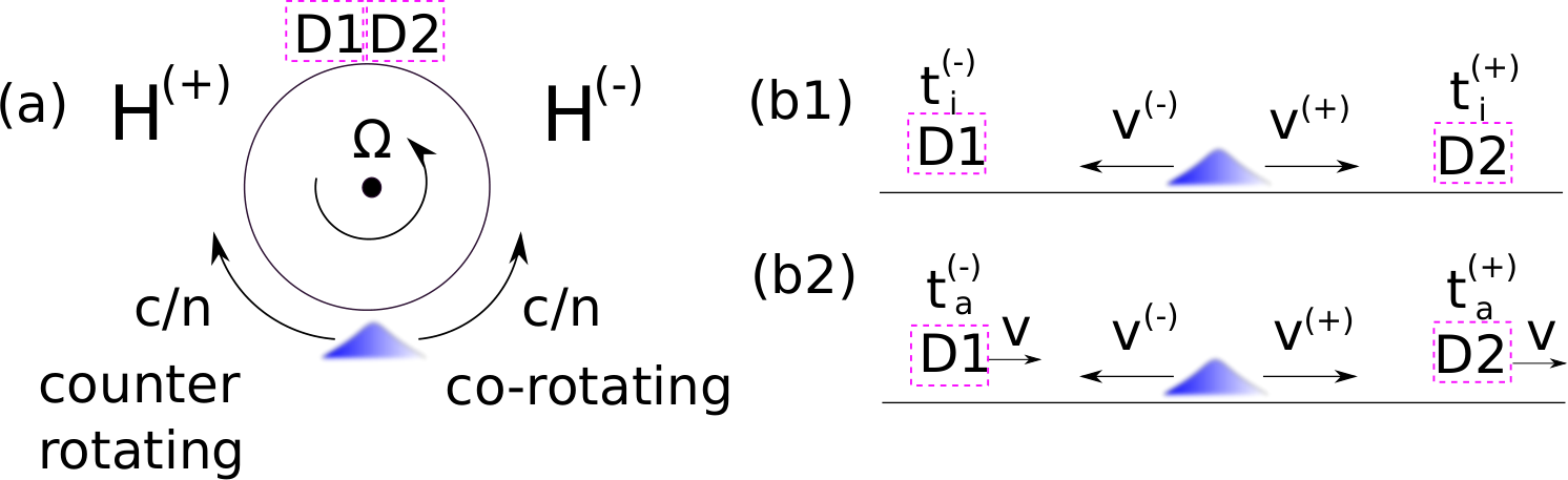
To describe quantum mechanically the evolution of the system we choose for convenience the viewpoint of the co-rotating observer (see Fig. 1(a)). To account for the non-inertial motion when we start from the Born chart and exploit the methods of symplectic Hamiltonian mechanics (4; 3). In particular, exploiting the so-called co-moment map from the generators of the Poincaré algebra to Hilbert space operators one finds the following Hamiltonian (see supplementary material):
| (1) |
where is the Lorentz factor. The term keeps track of the non-inertial motion of the detector, , which is the generator of translations, changes the relative distance between the detector and the system, e.g. in a time the relative distance changes by .
We now apply the Hamiltonian in Eq. (1) to photon-interferometry. We use the Abraham relation between kinetic momentum and energy (21; 22):
| (2) |
We combine Eqs. (1) and (2) to find:
| (3) |
where the positive (negative) superscript denotes the counter-rotating (co-rotating) motion to be measured by the detector D1 (D2), and . We note that Eq. (3) suggests a simple physical interpretation of the Hamiltonian as the relativistic Doppler-shifted energy of the system.
We can finally write the total Hamiltonian of the system:
| (4) |
where we have assumed that the photons moving in opposite directions do not interact, and denotes the identity operators. In summary, the total Hilbert space can be written as where () denotes the Hilbert space of the counter-rotating (co-rotating) modes.
The time parameter that keeps track of the dynamics through Schrödinger’s equation is ticking as a clock following the detectors’ motion; this is a direct consequence of the quantization procedure that leads to the Hamiltonian in Eq. (4). However, here we are mainly interested in the dominant effects where one can approximate the Lorentz factor as and the distances and times coincide to those measured by a ruler and a clock in the inertial laboratory frame.
Photon-interferometry experiments. We now further develop the model by adopting Glauber’s theory of photo-detection (23). Here we will focus on the experimental situation of photons with a coherence time that is short compared to the time resolution of the detectors, but temporal aspects could be easily taken into account (24; 25).
To analyze photon-interferometry experiments we will work in the Schrödinger picture (26), where we will denote the initial (final) state with the subscripts (). We consider the experimental situation where at time the photon is prepared in a state , and then constrained to move in a circular motion for a time resulting in a state , where is the traveled distance. Although one can always postulate a given initial state it is nonetheless instructive to compare the state , which is assumed to be generated by the apparatus co-rotating with the platform, with the state generated by the same apparatus when the platform is not rotating, i.e. when . In particular, it is reasonable to assume that the frequencies of the initial states generated in the two experimental situations differ by at most . However, such a difference in the initial state produces only sub-leading effects which are not amplified during time-evolution, as can be explicitly verified using the formulae we will develop. One can thus approximate the initial states generated on the rotating platform with the states that would be generated at .
The time-evolution is given by the usual Schrödinger equation with the Hamiltonian in Eq. (4), i.e.
| (5) |
where we have defined , and () is the counter (co-rotating) mode.
The state then interferes at a beam-splitter and one measures the outputs using two-detectors: the input modes are and and we denote the output modes by and . Here we consider the following relation between the input and output modes:
| (6) |
In particular, we are interested in the probability of detecting photons in the modes or . To this end, it is convenient to define the temporal modes (27):
| (7) |
where . In particular, we define the single-photon probability of detection as
| (8) |
with a similar definition for the probability for the output mode . In addition, we also define the the two-photon probability of detection
| (9) |
which gives the coincidence probability. For the case we speak of coalescence or HOM photon bunching and for we speak of photon anti-coalescence or anti-bunching. Classically, one is limited to values , making coincidence probabilities a valuable tool to assess the quantum nature of the electromagnetic field. Importantly, anti-symmetrization and photon anti-coalescence reveals hidden entanglement, as has already been demonstrated experimentally in a non-rotating setup (28).
We consider first the experimental situation with a generic single-photon input state:
| (10) |
where , are one-photon wavefunctions. From Eqs. (8) and (10), exploiting Eqs. (6) and (7), we find
| (11) |
where we have imposed the normalization of the state, i.e. . As an example let us consider the Quantum Sagnac experiment (8): a photon is prepared in a superposition of counter-propagating modes before interfering at the beam splitter (see supplementary material). Specifically, we consider the initial state in Eq. (10) with the one-photon wavefunctions , where is a Gaussian with mean frequency and bandwidth . After the time-evolution using Eq. (5) we have the state in Eq. (10) with and . Using Eq. (11), and making the further approximation , we find the single-photon detection probability:
| (12) |
where is the classical Sagnac delay, is the rotation frequency, is the encircled area, is the circle radius.
We next consider the two-photon state
| (13) |
where is the two-photon spectrum. From Eqs. (9) and (13), exploiting Eqs. (6), (7), we find
| (14) |
where we have imposed the normalization . As an example we consider the Hong-Ou-Mandel experiment on a rotating platform (9): two identical photons counter-propagate before interfering at a beam-splitter (see supplementary material). The experimentalist controls the initial time-delay of the mode ; the initial state is given by Eq. (13) with the two-photon spectrum . After the time-evolution we find the final state in Eq. (13) with
| (15) |
Using Eq. (14) we then immediately find the coincidence probability:
| (16) |
where is the classical Sagnac delay.
In the previous paragraph we have considered identical photons with a separable spectrum (7), but one could also consider identical frequency-entangled photons. For example, if we consider spontaneous parametric down conversion (SPDC) type I two-photon generation (29) we again find the coincidence probability in Eq. (16). It would thus seem that entanglement in combination with rotational motion leaves no trace on the photon coincidence rate, , measurement. We now further explore this question.
Manifestation of entanglement through rotation. Entanglement can manifest itself in a HOM coincidence rate measurement through anti-coalescence, i.e. . In particular, for a completely anti-symmetric spectrum, i.e. , one obtains perfect anti-coalescence, but even with a partially anti-symmetric spectrum one can have , thus witnessing entanglement. As we show below, this manifestation of entanglement may be susceptible to the motion of the interferometer.
We consider the experimental setup depicted in Fig. 2. As an initial state we consider a SPDC type I two-photon state (i.e. two photons with the same polarisation) with spectrum
| (17) |
where we have omitted the normalization. We note that the initial spectrum in Eq. (17) is completely symmetric, i.e. , and gives at .
We now consider the same setup with the interferometer in a constant rotational motion with frequency . The final spectrum of the two-photon state changes to
| (18) |
where the factor results from the interference of the mode ; by ‘final state’ we again mean the state that arrives at the last beam-splitter. Using Eq. (14) we then find the coincidence probability
| (19) |
We have plotted as a function of the angular frequency in Fig. 3 with the interferometer area (assuming the photons travel through a 100 m long fibre, wound 35 times along a 0.9 m diameter loop) and Hz, corresponding to a typical photon carrier wavelength of 800 nm. Two curves are shown for two different photon bandwidths, Hz (blue solid curve) and Hz (dashed red curve), corresponding to 5 nm and 40 nm, respectively. The shaded region corresponding to indicates the presence of entanglement that manifests as photon anti-coalescence. Short bandwidth, i.e. long coherence photons show a periodic series of revivals of entanglement with increasing rotation frequency. For larger photon bandwidths, i.e. shorter coherence lengths, increasing the relative photon delay by increasing the rotation speed leads to a reduction of the coincidence peak values and of the overall fringe visibility. This is a result of the loss of mutual coherence between the two interfering photons.
The anti-symmetrization of the photon spectrum, which leads to a modification of the coincidence probability, is a direct consequence of the non-inertial motion of platform. More generally, this shows that rotational motion can activate dormant asymmetries in the experimental setup leading to an anti-symmetric spectrum. It is also interesting to consider an initial anti-symmetric spectrum ; the proposed experiment shows that can become symmetrized during time-evolution, fully concealing the anti-coalescence signature of entanglement.
These effects can be traced to the impossibility of clock synchronization along a closed loop on the rotating platform. In particular, the Hamiltonian in Eq. (5) can be linked to the effect of clock desynchronization (2). It is important to note that this is a genuine relativistic effect, which is not expected to arise in a Newtonian theory, although it imprints a non-negligible experimental trace in the regime typically associated with the latter. This is different from the observer-dependent entanglement effect in non-inertial reference frames (30), expected to arise as a consequence of the Unruh radiation (31; 32) which vanishes at low accelerations.
Conclusions. We have developed a formalism for describing interferometry experiments on rotating platforms. We have first analyzed two recent photon-interferometry experiments, namely, the quantum Sagnac and the Hong-Ou-Mandel experiment on a rotating platform. We have then proposed a modified Hong-Ou-Mandel interferometer where entanglement can be revealed or concealed depending on the rotational frequency. These results indicate new directions for investigating the notions of space and time as well as its consequences in a quantum mechanical regime.
Acknowledgments. The authors acknowledge support from the EU H2020FET project TEQ (Grant No. 766900), from the EPSRC (UK, Grant No. EP/M009122/1) and from the European Union’s Horizon 2020 research and innovation programme under grant agreement No 820392.
References
- (1) Hermann Minkowski. Raum und zeit. Jahresbericht der Deutschen Mathematiker-Vereinigung, vol. 18, p. 75-88, 18:75–88, 1909.
- (2) Vesselin Petkov et al. Minkowski spacetime: A hundred years later, volume 11. Springer, 2010.
- (3) WA Von Ignatowsky. Einige allgemeine bemerkungen zum relativitätsprinzip. Verh. Deutsch. Phys. Ges, 12:788–796, 1910.
- (4) Stefano Liberati. Tests of lorentz invariance: a 2013 update. Classical and Quantum Gravity, 30(13):133001, 2013.
- (5) Howard P Robertson. Postulate versus observation in the special theory of relativity. Reviews of modern Physics, 21(3):378, 1949.
- (6) Albert A Michelson and Edward W Morley. On the relative motion of the earth and of the luminiferous ether. Sidereal Messenger, vol. 6, pp. 306-310, 6:306–310, 1887.
- (7) Chong-Ki Hong, Zhe-Yu Ou, and Leonard Mandel. Measurement of subpicosecond time intervals between two photons by interference. Physical review letters, 59(18):2044, 1987.
- (8) Leonard Mandel. Quantum effects in one-photon and two-photon interference. In More Things in Heaven and Earth, pages 460–473. Springer, 1999.
- (9) Ashley Lyons, George C Knee, Eliot Bolduc, Thomas Roger, Jonathan Leach, Erik M Gauger, and Daniele Faccio. Attosecond-resolution hong-ou-mandel interferometry. Science advances, 4(5):eaap9416, 2018.
- (10) Éric Gourgoulhon. Special relativity in general frames. Springer, 2016.
- (11) Georges Sagnac. L’éther lumineux démontré par l’effet du vent relatif d’éther dans un interféromètre en rotation uniforme. CR Acad. Sci., 157:708–710, 1913.
- (12) Georges Sagnac. Sur la preuve de la réalité de l’éther lumineux par l’expérience de l’interférographe tournant. CR Acad. Sci., 157:1410–1413, 1913.
- (13) Evert Jan Post. Sagnac effect. Reviews of Modern Physics, 39(2):475, 1967.
- (14) Matthias Fink, Ana Rodriguez-Aramendia, Johannes Handsteiner, Abdul Ziarkash, Fabian Steinlechner, Thomas Scheidl, Ivette Fuentes, Jacques Pienaar, Timothy C Ralph, and Rupert Ursin. Experimental test of photonic entanglement in accelerated reference frames. Nature communications, 8:15304, 2017.
- (15) Matthias Fink, Fabian Steinlechner, Johannes Handsteiner, Jonathan P Dowling, Thomas Scheidl, and Rupert Ursin. Entanglement-enhanced optical gyroscope. New Journal of Physics, 21(5):053010, 2019.
- (16) Sara Restuccia, Marko Toroš, Graham M. Gibson, Hendrik Ulbricht, Daniele Faccio, and Miles J. Padgett. Photon bunching in a rotating reference frame. Phys. Rev. Lett., 123:110401, Sep 2019.
- (17) Guillaume Bertocchi, Olivier Alibart, Daniel Barry Ostrowsky, Sébastien Tanzilli, and Pascal Baldi. Single-photon sagnac interferometer. Journal of Physics B: Atomic, Molecular and Optical Physics, 39(5):1011, 2006.
- (18) Angelo Tartaglia and Matteo Luca Ruggiero. The sagnac effect and pure geometry. American Journal of Physics, 83(5):427–432, 2015.
- (19) Ana Cannas Da Silva and A Cannas Da Salva. Lectures on symplectic geometry, volume 3575. Springer, 2001.
- (20) Peter Woit, Woit, and Bartolini. Quantum Theory, Groups and Representations. Springer, 2017.
- (21) Miles J Padgett. On diffraction within a dielectric medium as an example of the minkowski formulation of optical momentum. Optics express, 16(25):20864–20868, 2008.
- (22) Stephen M Barnett. Resolution of the abraham-minkowski dilemma. Physical review letters, 104(7):070401, 2010.
- (23) Roy J Glauber. The quantum theory of optical coherence. Physical Review, 130(6):2529, 1963.
- (24) Thomas Legero, Tatjana Wilk, Axel Kuhn, and Gerhard Rempe. Characterization of single photons using two-photon interference. Advances In Atomic, Molecular, and Optical Physics, 53:253–289, 2006.
- (25) Holger P Specht, Jörg Bochmann, Martin Mücke, Bernhard Weber, Eden Figueroa, David L Moehring, and Gerhard Rempe. Phase shaping of single-photon wave packets. Nature Photonics, 3(8):469, 2009.
- (26) Kaige Wang. Quantum theory of two-photon wavepacket interference in a beamsplitter. Journal of Physics B: Atomic, Molecular and Optical Physics, 39(18):R293, 2006.
- (27) KJ Blow, Rodney Loudon, Simon JD Phoenix, and TJ Shepherd. Continuum fields in quantum optics. Physical Review A, 42(7):4102, 1990.
- (28) Alessandro Fedrizzi, Thomas Herbst, Markus Aspelmeyer, Marco Barbieri, Thomas Jennewein, and Anton Zeilinger. Anti-symmetrization reveals hidden entanglement. New Journal of Physics, 11(10):103052, 2009.
- (29) Marco Barbieri, Emanuele Roccia, Luca Mancino, Marco Sbroscia, Ilaria Gianani, and Fabio Sciarrino. What hong-ou-mandel interference says on two-photon frequency entanglement. Scientific reports, 7(1):7247, 2017.
- (30) Ivette Fuentes-Schuller and Robert B Mann. Alice falls into a black hole: entanglement in noninertial frames. Physical review letters, 95(12):120404, 2005.
- (31) Paul CW Davies. Scalar production in schwarzschild and rindler metrics. Journal of Physics A: Mathematical and General, 8(4):609, 1975.
- (32) William G Unruh. Notes on black-hole evaporation. Physical Review D, 14(4):870, 1976.
Supplementary material to “Revealing and concealing entanglement with non-inertial motion”
S1: Laboratory reference frame
In this section we briefly discuss the relation between the co-rotating reference frame and the inertial laboratory reference frame, focusing on the classical effects. We start by noting that the speed of light in the co-rotating reference frame, where the co-rotating medium is stationary, is the same in the co-rotating and counter-rotating directions; specifically we have that the velocities are . Using the relativistic velocity addition formula we find the corresponding velocities in the inertial laboratory frame:
| (S1) |
where , and . The corresponding speeds are given by . See Fig. 1(b) for a graphical illustration of this light-dragging effect, which coincides with the Fizeau effect, but could in principle differ (1).
We assume an initial spatial-distance between the systems and the detectors. We can convert into a time-distance, i.e. the initial time-distance (see Fig. 1(b1)), which is given by . Furthermore, exploiting Eq. (S1), we find:
| (S2) |
However this is different from the actual time it takes the signals to reach the detectors (see Fig. 1 (b2)): we need to take into account also the motion of the detectors. In particular we have the condition which after some algebra readily gives
| (S3) |
In this way we immediately recover the classic Sagnac delay given by . Specifically, to find the usual expression of the Sagnac delay we set , where denotes the winding number, and define the encircled area as . Using we then immediately find (1; 2):
| (S4) |
From this discussion it is clear why the description in the co-rotating reference frame is slightly more convenient: there only the non-inertial motion of the detectors has to be taken into account (through the Hamiltonians). On the other hand, in the laboratory inertial reference frame, one has to account for the motion of the detectors as well as of the medium (again through the Hamiltonians). In short, the advantage of the co-rotating reference frame is the absence of the light-dragging effect.
The Sagnac delay can be obtained also from the perspective of the co-rotating observer where it arises from clock desynchronization (2).
S2: Derivation of the Hamiltonian
In this section we derive the Hamiltonian for the experiments depicted in Fig. 1(a): we consider a rotating platform, which spins at angular frequency , and we restrict to the dynamics on a circle of radius , centered on the symmetry axis of the rotating platform. Specifically, we will adopt the methods of representation theory (3) and symplectic Hamiltonian mechanics (4) to map the time-evolution generator of the Poincaré algebra to a Hilbert space operator. One could of course make an ad-hoc quantization in a non-inertial reference frame, and obtain a Hamiltonian, but the results might be inconsistent with basic symmetry requirements. Anyhow, we choose the former method which constructs the Hamiltonian starting from basic symmetry considerations of the Poincaré group. As argued in the supplemental material S1 we will for convenience describe the experiment in the co-rotating reference frame.
One typically starts describing the experiments by setting up a chart, e.g. a Cartesian chart. We note that the chosen spacetime coordinates critically reflect the motion of the observer which affects the resulting description of the dynamics. For example, two observers moving with different speeds or accelerations will use different charts, and hence ascribe different energies to the same system, and hence care must be taken with the choice of the coordinate system. In the following we will assume that the detectors are stationary in the observer’s chart: with this choice there is a simple relation between observables in the description and the quantities measured by the detectors.
We start by recalling the quantization procedure in an inertial reference frame, i.e. with . In our case, we will use the polar chart for the laboratory inertial reference frame. Specifically, the line-element in an inertial reference frame expressed in the polar chart is given by
| (S5) |
where is a constant in our case (we have restricted the analysis to a spacetime). From the line-element in Eq. (S5) it is then possible to immediately read the time-evolution Killing vector (5). The time-evolution Killing vector (more precisely a vector field) is the tangent vector to the flow lines of a system in free motion. Using the co-moment map we can then map the time-evolution Killing vector to the Hilbert space Hamiltonian (3; 4):
| (S6) |
where is the representation of the time-evolution generator on the considered Hilbert space. For example, for a single mode we would have , where is the frequency of the oscillator.
To apply the quantization procedure in a non-inertial reference frame, i.e. with , we have to make an additional step: we have to relate the co-rotating reference frame to the laboratory inertial reference frame. There reason is simple: we do not know how to directly quantize in a non-inertial reference frame, but only in the inertial reference frame. We denote the laboratory (polar) and the co-rotating (Born) coordinates by the unprimed () and primed () labels, respectively. In particular, we have the following relation (6):
| (S7) | ||||
| (S8) |
It is straightforward to find the corresponding transformation matrix
and to express the Minkowski metric in the two coordinates systems, i.e.
| (S11) | ||||
| (S12) |
From Eqs. (S11) and (S12) we can immediately find the relevant Killing vectors , , and . Using Eq. (S2: Derivation of the Hamiltonian) we can then express in the laboratory coordinates, i.e.
| (S13) |
which gives , and thus
| (S14) |
We have now expressed the time-evolution Killing vector , which generates the dynamics in the co-rotating reference frame, in terms of the Killing vectors and , which generate time-evolution and space-translation in the inertial laboratory reference frame, respectively. We can now map the latter Killing vectors to operators on a Hilbert space using the usual prescription
| (S17) |
which we name Born Hamiltonian. Note that Eq. (S17) captures the idea that the dynamics on a rotating platform can be fully explained in terms of the non-inertial motion of the detector (7): the term describes the non-inertial motion of the detector, i.e. at each instant of time the detector is translated with respect to the system which evolves freely on a circle.
We note that the transformation in Eq. (S7) leaves the time coordinate unchanged. This can be seen as a Galilean-type transformation on a circle, which we now generalize to a Lorentz-type transformation. In particular, we consider
| (S18) | ||||
| (S19) |
where . If we set and the transformation is formally equivalent to a Lorentz boost with speed , while if we set and we obtain the transformation considered by Post (1). We find that the Hamiltonian is insensitive to the value of , but depends on the chosen value of . In the following we set which leads to the Hamiltonian
We can also analyze non-uniform rotations using the above formalism by considering a time-dependent angular frequency (we remark that the time-evolution vector does not need to be generally a Killing vector). We repeat the derivation in this section with the formal replacements
| (S21) | ||||
| (S22) |
At the end we obtain in place of Eq. (S20) the following Hamiltonian:
| (S23) |
In this case one expects two physical effects, one related to the (geometrical) Sagnac phase, and a possible new contribution related to a dynamical phase, which typically emerges in situations where there is a time-dependence in the Hamiltonian.
S3: Notes on experimental setups
In this section we summarize the two experimental schemes that form the building blocks, conceptually as well as experimentally, for the new proposal to demonstrate how entanglement can be revealed or concealed with non-inertial motion. The Quantum Sagnac experiment is depicted in Fig. S1(a): a photon enters through the path 1, is directed into path 2 and then interferes for the first time with the beam splitter. After evolving in counter-progating directions, the photon then interferes again at the beam splitter, after which it is detected. The Hong-Ou-Mandel experiment on a rotating platform is depicted in Fig. S1(b): two identical photons counter-propagate before interfering at a beam-splitter. One detects the arrival of the photons and extracts the coincidence probability, . In both cases, the setups are placed on a rotating platform.
The proposal shown in Fig. 2 can be seen as a combination of the setups shown in Fig. S1, which can be exploited to gain an intuitive understanding of the results. For example, the asymptotic value for the coincidence probability in Fig. 3 can be intuitively understood in terms of Quantum Sagnac and the HOM setups. From Eq. (19) we find at high rotation frequency the value ; this is halfway between a full dip, , and the case without bunching or anti-bunching, . The paths denoted by the purple and blue arrows in Fig. 2 can be related to the Quantum Sagnac: at high rotation frequency the counter-propagating mode (blue arrow) no longer interferes with the co-rotating modes due to non-overlapping frequency spectra. Loosely speaking, the counter-propagating mode (blue arrow) can be heuristically associated to half of the initial mode , while the other half of the mode co-rotates (purple arrow) and interferes with the other co-rotating mode (green arrow). As the frequency spectrum of the two co-rotating modes is identical, i.e. no time-delay exists between them, they bunch together at the output ports of the beam-splitter. Hence the counter-rotating (co-rotating) part of the mode is associated with (). The coincidence probability at high rotation frequency can be thus seen as the average behaviour, i.e. .
References
- (1) Evert Jan Post. Sagnac effect. Reviews of Modern Physics, 39(2):475, 1967.
- (2) Éric Gourgoulhon. Special relativity in general frames. Springer, 2016.
- (3) Peter Woit, Woit, and Bartolini. Quantum Theory, Groups and Representations. Springer, 2017.
- (4) Ana Cannas Da Silva and A Cannas Da Salva. Lectures on symplectic geometry, volume 3575. Springer, 2001.
- (5) Eric Poisson. A relativist’s toolkit: the mathematics of black-hole mechanics. Cambridge university press, 2004.
- (6) Guido Rizzi and Matteo Luca Ruggiero. Space geometry of rotating platforms: an operational approach. Foundations of Physics, 32(10):1525–1556, 2002.
- (7) Angelo Tartaglia and Matteo Luca Ruggiero. The sagnac effect and pure geometry. American Journal of Physics, 83(5):427–432, 2015.
- (8) Guillaume Bertocchi, Olivier Alibart, Daniel Barry Ostrowsky, Sébastien Tanzilli, and Pascal Baldi. Single-photon sagnac interferometer. Journal of Physics B: Atomic, Molecular and Optical Physics, 39(5):1011, 2006.
- (9) Sara Restuccia, Marko Toroš, Graham M. Gibson, Hendrik Ulbricht, Daniele Faccio, and Miles J. Padgett. Photon bunching in a rotating reference frame. Phys. Rev. Lett., 123:110401, Sep 2019.