Multi-Antenna Aided Secrecy Beamforming Optimization for Wirelessly Powered HetNets

Shiqi Gong Shaodan Ma Chengwen Xing Yonghui Li Lajos Hanzo

Abstract

The new paradigm of wirelessly powered two-tier heterogeneous networks (HetNets) is considered in this paper. Specifically, the femtocell base station (FBS) is powered by a power beacon (PB) and transmits confidential information to a legitimate femtocell user (FU) in the presence of a potential eavesdropper (EVE) and a macro base station (MBS). In this scenario, we investigate the secrecy beamforming design under three different levels of FBS-EVE channel state information (CSI), namely, the perfect, imperfect and completely unknown FBS-EVE CSI. Firstly, given the perfect global CSI at the FBS, the PB energy covariance matrix, the FBS information covariance matrix and the time splitting factor are jointly optimized aiming for perfect secrecy rate maximization. Upon assuming the imperfect FBS-EVE CSI, the worst-case and outage-constrained SRM problems corresponding to deterministic and statistical CSI errors are investigated, respectively. Furthermore, considering the more realistic case of unknown FBS-EVE CSI , the artificial noise (AN) aided secrecy beamforming design is studied. Our analysis reveals that for all above cases both the optimal PB energy and FBS information secrecy beamformings are of rank-1. Moreover, for all considered cases of FBS-EVE CSI, the closed-form PB energy beamforming solutions are available when the cross-tier interference constraint is inactive. Numerical simulation results demonstrate the secrecy performance advantages of all proposed secrecy beamforming designs compared to the adopted baseline algorithms.

I Introduction

With the proliferation of smart devices and data-hungry applications, establishing ubiquitous, high-throughput and secure communications is gaining increased importance in next-generation systems [1, 2, 3]. The traditional macrocells generally have poor performance in terms of indoor coverage and cell edge rate. To tackle this issue, heterogenous networks (HetNets) have emerged as a promising next-generation architecture, which are generally supported by heterogenous base stations (BSs) having different service coverages [4, 5]. Specifically, the macrocell base station (MBS) can provide open access and wide coverage up to dozens of kilometers, while the low-power femtocell base station (FBS) and picocell base station (PBS) are typically deployed in indoor environments and near to femtocell users (FUs) and picocell users (PUs), respectively. As pointed out in [6], the ultra-dense deployment of femtocells is recognized as an effecient technique to realize 1000 times increase in wireless data rate for. However, due to the high spatial spectrum reuse in HetNets and the dense deployment of FBSs and PBSs, cross-tier interference is usually unavoidable in HetNets. Fortunately, according to [7, 8], the interference can be re-utilized as an effective radio-frequency (RF) energy source for wireless energy harvesting (WEH), which thus contributes to the green and self-sustainable communications. WEH has many advantages over conventional energy supply methods [9]. For example, WEH is more reliable than natural energy supply, such as solar, wind and tide, which are significantly affected by climate and terrain. Also, it is more cost-effective compared to the widely adopted batteries recharge/replacement technique. Generally, the densely deployed HetNets are favorable from the perspective of improving efficiency of WEH, since the distances from energy harvesters to energy stations are substantially shortened.

Recently, WEH-based HetNets have received extension attention, in which the power beacons (PBs) provide power for other nodes via wireless energy transfer [10, 11, 12, 13, 14, 15, 16]. In [10], H. Tabassum and E. Hossain studied the optimal deployment of PBs in wirelessly powered cellular networks. In [11], the downlink resource allocation problem was investigated by S. Lohani et al. under both time-switching and power-splitting based simultaneous wireless information and power transfer (SWIPT) strategies for two-tier HetNets. The comprehensive analysis of the outage probability and the average ergodic rate in both downlink and uplink stages of wirelessly powered HetNets with different cell associations were presented by S. Akbar et al. in [12]. Y. Zhu et al. in [13] further extended the above work into the Massive MIMO aided HetNets with WEH, where different user association schemes are investigated in terms of the achievable average uplink rate. From the view of green communications, the energy efficient beamforming designs for SWIPT HetNets was studied by M. Sheng et al. and H. Zhang et al. in [14] and [15], respectively. To increase energy harvesting efficiency multi-antenna PBs and users, J. Kim et al. in [16] considered sum throughput maximization under different cooperative protocols of two-tier wireless powered cognitive networks.

Furthermore, owing to the open network architectures of HetNets, the security issue faced by wireless powered HetNets has also drawn extensive attention [17]. As a mature technique to guarantee secure communications from the information-theoretical perspective, physical-layer security (PLS) has been widely researched in both academia and industry [18, 19]. There have been some works considering applying PLS techniques to HetNets with WEH. In [20] and [21], the artificial noise based secrecy rate maximization was studied for secure HetNets with SWIPT. The authors in [22] proposed the max-min secrecy energy efficiency optimization for wireless powered HetNets, and a distributed ADMM approach was applied to reduce the information exchange overhead. Considering the more practical scenarios where the transmitter only has imperfect eavesdropper’s CSI, a secrecy SWIPT strategy for two-tier cognitive radio networks was investigated in [23].

Most of the existing works on HetNets with WEH focus on SWIPT HetNets, it is still an open challenging issue on how to design the optimal harvest-then-transmit strategies for HetNets. In this paper, we investigate the secrecy beamforming design for a wirelessly powered HetNet, where the wirelessly powered FBS transmits the confidential information to a single-antenna FU in the presence of a multi-antenna eavesdropper (Eve). The FBS can harvest energy from the PB and the MBS. Moreover, there is no cooperation among the MBS, the PB and the FBS, thus the resultant cross-tier interference is taken into account. In this wirelessly powered HetNet, the energy and information covariance matrices as well as the time splitting factor are jointly optimized to maximize the secrecy rate under different levels of FBS-EVE CSI. Our main contribution is summarized as :

•

Firstly, we study secrecy rate maximization (SRM) of the wirelessly powered HetNet having perfect global CSI. In order to address this non-convex perfect SRM problem, a relaxed problem using the matrix trace inequality is studied and proved to be tight, since it always provides a rank-1 optimal solution. Considering the joint-convexity and quasi-convexity of the relaxed problem on different variables, a convexity-based linear search is proposed for optimally solving the perfect SRM problem. In particular, the closed-form solution of this problem is derived when the cross-tier interference at the MU is negligible.
•

Secondly, the imperfect FBS-EVE CSI with deterministic and Gaussian random CSI errors are considered, respectively. For the deterministic CSI error, the worst-case SRM problem is studied, which can be addressed similarly to the perfect SRM problem using the S-procedure. For the Gaussian random CSI error, the outage-constrained SRM problem subject to the probabilistic secrecy rate constraint is studied by applying the Bernstein-type inequality (BTI) [24] and then an alternating optimization procedure is proposed. For both the worst-case and the outage-constrained SRM problems, the rank-1 property of the optimal solutions is also validated.
•

Finally, we consider the realistic scenario with unknown FBS-EVE CSI, in which artificial noise (AN) is utilized for improving secrecy performance. We design AN aided secrecy beamforming by maximizing the average AN power subject to the legitimate rate requirement at the FU. This robust design can be reformulated as a concave one and its optimal rank-1 solution is demonstrated. Similarly, for the inactive cross-interference constraint, the closed-form solution to this AN aided secrecy beamforming design is available.

In fact, the studied SRM problems belong to the nonconvex difference of convex functions (DC) programming, which are more challenging than that in [16] focusing on the sum-throughput maximization of cognitive WPCNs. Compared to the SRM problem of [25] where the single-antenna PB and Eve are assumed, these SRM problems are also more intractable due to the additional energy and interference constraints. Fortunately, we validate that the optimal energy and information beamformings are of rank-1 in the secrecy wirelessly powered HetNet, regardless of the availability of eavesdropper’s CSI. This conclusion also provides important insights for practical engineering applications.

Notations: The bold-faced lower-case and upper-case letters stand for vectors and matrices, respectively. The operators $(\cdot)^{\rm T}$ , $(\cdot)^{\rm H}$ and $(\cdot)^{-1}$ denote the transpose, Hermitian and inverse of a matrix, respectively. $\text{Tr}(\bm{A})$ and $\det(\bm{A})$ represent the trace and determinant of $\bm{A}$ , respectively. $\|\cdot\|_{2}$ denotes the matrix spectral norm and $\bm{A}\!\succeq\!\bm{0}$ indicates that the square matrix $\bm{A}$ is positive semidefinite. $\text{rank}(\bm{A})$ and $\nu({\bf A})$ denote the rank of ${\bf A}$ and the unit-norm eigenvector associated with the maximum eigenvalue of ${\bf A}$ , respectively. Also, $(a)^{+}\!=\!\max\{a,0\}$ is defined. The words ‘independent and identically distributed’ and ‘with respect to’ are abbreviated as ‘i.i.d.’ and ‘w.r.t.’, respectively.

II System model and Problem Formulation

As shown in Fig. 1, we consider secure communications of the wirelessly powered HetNet, in which an $N_{M}$ -antenna MBS used for information transmission coexists with an $N_{P}$ -antenna PB deployed for wireless energy transfer and an $N_{F}$ -antenna FBS aiming for energy harvesting. Note that the FBS is

Refer to caption — Fig. 1: A secrecy wirelessly powered HetNet.

energy-limited and harvests energy for its communications from the RF signals transmitted by the PB and the MBS. The MBS and the PB transmit the information-bearing signal ${\bf s}_{M}\in\mathbb{C}^{N_{M}}$ and energy-bearing signal ${\bf{s}}_{P}\in\mathbb{C}^{N_{P}}$ to a single-antenna MU and an $N_{F}$ -antenna FBS, respectively. Then the FBS transmits the confidential signal ${\bf s}_{F}\in\mathbb{C}^{N_{F}}$ to a single-antenna FU, while a multi-antenna Eve aims for intercepting the signal of the FBS. We focus our attention on the security of FBS and there is no cooperation between the MBS and the FBS. Hence, the signals transmitted from the MBS and the FBS actually impose interference on the FU and the MU, respectively. All wireless channels are assumed to be quasi-static flat-fading and remain constant during a whole time slot $T$ .

In the initial $\tau T$ subslot, where $0<\tau<1$ denotes the time splitting factor, the FBS harvests energy from both the PB energy signal ${\bf s}_{P}$ and MBS interfering signal ${\bf s}_{M}$ . Let’s define ${\bf W}_{P}=\mathbb{E}[{\bf s}_{P}{\bf s}_{P}^{H}]\!\in\!\mathbb{C}^{N_{P}\times N_{P}}$ as the covariance matrix of the PB energy signal ${\bf s}_{P}$ subject to the maximum transmit power $P_{P}$ , i.e. $\text{tr}({\bf W}_{P})\leq P_{P}$ , and for simplicity $\mathbb{E}[{\bf s}_{M}{\bf s}_{M}^{H}]=\frac{P_{M}}{N_{M}}{\bf I}_{N_{M}}$ with $P_{M}$ being the MBS maximum transmit power. By neglecting the contribution of thermal noise to the total harvested energy at the FBS, the amount of energy harvested at the FBS is expressed as

\displaystyle E({\bf W}_{P})=\tau T\xi\big(\text{tr}({\bf H}_{F}{\bf W}_{P}{\bf H}_{F}^{H})+\frac{P_{M}}{N_{M}}\text{tr}({\bf G}_{F}{\bf G}_{F}^{H})\big)

(1)

where $0<\xi<1$ is the energy harvesting efficiency factor. ${\bf H}_{F}\in\mathbb{C}^{N_{F}\times N_{P}}$ and ${\bf G}_{F}\in\mathbb{C}^{N_{F}\times N_{M}}$ denote the PB-FBS channel and MBS-FBS channel, respectively.

Next, in the second $(1-\tau)T$ subslot, the FBS transmits the confidential signal ${\bf s}_{F}$ to the FU by utilizing the harvested energy in (1). The signals received at the FU and the Eve are then expressed as

		$\displaystyle{y}_{R}={\bf h}_{R}^{H}{\bf s}_{F}+{\bf g}_{R}^{H}{\bf s}_{M}+{n}_{R},$
		$\displaystyle{\bf y}_{E}={\bf H}_{E}{\bf s}_{F}+{\bf G}_{E}{\bf s}_{M}+{\bf n}_{E},$		(2)

where ${\bf h}_{R}\in\mathbb{C}^{N_{F}}$ and ${\bf g}_{R}\in\mathbb{C}^{N_{M}}$ denote the FBS-FU channel and the MBS-FU channel, respectively. ${\bf H}_{E}\in\mathbb{C}^{N_{E}\times N_{F}}$ and ${\bf G}_{E}\in\mathbb{C}^{N_{E}\times N_{M}}$ denote the FBS-EVE channel and the MBS-EVE channel, respectively. $n_{R}\sim\mathcal{CN}({0,\sigma_{n}^{2}})$ and ${\bf n}_{E}\sim\mathcal{CN}({\bf 0},\sigma_{n}^{2}{\bf I}_{N_{E}})$ are i.i.d circularly symmetric Gaussian noises at the FU and the EVE, respectively. Additionally, we define ${\bf P}_{F}=\mathbb{E}[{\bf s}_{F}{\bf s}_{F}^{H}]\!\in\!\mathbb{C}^{N_{F}\times N_{F}}$ as the covariance matrix of the FBS information signal ${\bf s}_{F}$ , the achievable rates (in bps/Hz) at the FU and the EVE are then given by

		$\displaystyle R_{I}=(1-\tau)\log_{2}\bigg(1+\frac{{\bf h}_{R}^{H}{\bf P}_{F}{\bf h}_{R}}{\sigma_{n}^{2}+\frac{P_{M}}{N_{M}}\\|{\bf g}_{R}\\|^{2}}\bigg),$
		$\displaystyle R_{E}=(1-\tau)\log_{2}\det\big({{\bf I}}_{N_{E}}\!+\!(\sigma_{n}^{2}{\bf I}_{N_{E}}+\frac{P_{M}}{N_{M}}{\bf G}_{E}{\bf G}_{E}^{H})^{-1}\!{\bf H}_{E}{\bf P}_{F}{\bf H}_{E}^{H}\big).$		(3)

According to [20], the achievable secrecy rate $R_{S}$ of the wirelessly powered HetNet is actually the data rate at which the desired information is correctly decoded by the FU, while no information is wiretapped by the EVE. Mathematically, we have

\displaystyle R_{S}=[R_{I}-R_{E}]^{+}.

(4)

In our work, we jointly optimize the PB and FBS transmit covariance matrices $\{{\bf W}_{P},{\bf P}_{F}\}$ and the time splitting factor $\tau$ for maximizing the achievable secrecy rate $R_{S}$ in (4). The resultant SRM problem for the wirelessly powered HetNet is then formulated as

		$\displaystyle{R}_{S}^{\star}=\underset{{{\tau},{\bf W}_{P}\succeq{\bf 0},{\bf P}_{F}\succeq{\bf 0}}}{\text{max}}~~R_{I}-R_{E}$
		$\displaystyle~{\rm{s.t.}}~~\text{CR1:}~0\leq\tau\leq 1,~\text{tr}({\bf W}_{P})\leq P_{P}$
		$\displaystyle~~~~~~~\text{CR2:}~(1\!-\!\tau)\text{tr}({\bf P}_{F})\!\leq\!\tau\xi\big[\text{tr}({\bf H}_{F}{\bf W}_{P}{\bf H}_{F}^{H})+\frac{P_{M}}{N_{M}}\text{tr}({\bf G}_{F}{\bf G}_{F}^{H})\big],$
		$\displaystyle~~~~~~~\text{CR3:}~\tau{\bf h}_{M}^{H}{\bf W}_{P}{\bf h}_{M}+(1\!-\!\tau){\bf g}_{p}^{H}{\bf P}_{F}{\bf g}_{p}\!\leq\!I_{th}.$		(5)

In problem (II), the constraint CR1 comes from the fact that the PB transmit power has a maximum threshold, and CR2 denotes the energy causality constraint of the wirelessly powered FBS. While CR3 models the average interference constraint of the secrecy wirelessly powered HetNet. Specifically, by defining ${\bf h}_{M}\in\mathbb{C}^{N_{P}}$ and ${\bf g}_{p}\in\mathbb{C}^{N_{F}}$ as the PB-MU channel and the FBS-MU channel, respectively, the terms ${\bf h}_{M}^{H}{\bf W}_{P}{\bf h}_{M}$ and ${\bf g}_{p}^{H}{\bf P}_{F}{\bf g}_{p}$ actually denote the total interference at the MU originating from the PB and the FBS, respectively. Since the PB energy transfer and the FBS information transfer are separated by the time splitting factor $\tau$ , we consider the average interference power constraint at the MU as shown in CR3, where $I_{th}$ denotes the minimum tolerable interference. It is readily inferred from CR3 that problem (II) is feasible for an arbitrary $I_{th}\geq 0$ . However, due to the highly coupled variables $\{{\tau},{\bf W}_{P},{\bf P}_{F}\}$ , the SRM problem (II) is generally non-convex and challenging to address.

In the sequel, we will investigate the SRM under three different levels of the FBS-EVE CSI. In the first case, the global CSI of the wirelessly powered HetNet is available at the FBS via channel feedback and high-SNR training techniques. In the second case, by assuming imperfect FBS-EVE CSI at the FBS, a pair of robust SRM problems are investigated under deterministic and Gaussian random CSI errors, respectively. In the third case, we consider the more practical scenario that the FBS is not aware of the existence of Eve. In other words, the FBS-EVE CSI is completely unknown to the FBS.

III Perfect SRM under global CSI of the wirelessly powered HetNet

In this section, a convexity-based one dimensional search is proposed for optimally solving the SRM problem (II) under the global CSI of the wirelessly powered HetNet.

III-A Transformation of Problem (II)

Firstly, by introducing an auxiliary variable $\eta$ , the SRM problem (II) can be reformulated as

		$\displaystyle{R}_{S}^{\star}=\underset{\begin{subarray}{c}{\tau},{\bf W}_{P}\succeq{\bf 0},{\bf P}_{F}\succeq{\bf 0},\eta\end{subarray}}{\text{max}}~(1-\tau)\log_{2}\bigg(1+{C_{1}{\bf h}_{R}^{H}{\bf P}_{F}{\bf h}_{R}}\bigg)\!-\!(1\!-\!\tau)\log_{2}\eta$
		$\displaystyle{\rm{s.t.}}~~\text{CR1}\sim\text{CR3},~~~\text{CR4:}~\det\big({{\bf I}}_{N_{E}}\!+\!{\bf R}_{E}{\bf H}_{E}{\bf P}_{F}{\bf H}_{E}^{H}\big)\leq\eta,$		(6)

where $C_{1}={(\sigma_{n}^{2}+\frac{P_{M}}{N_{M}}\|{\bf g}_{R}\|^{2})^{-1}}$ and ${\bf R}_{E}=(\sigma_{n}^{2}{\bf I}_{N_{E}}+\frac{P_{M}}{N_{M}}{\bf G}_{E}{\bf G}_{E}^{H})^{-1}$ . Unfortunately, problem (III-A) is still difficult to address because of the nonconvex constraint CR4. In order to tackle this issue, we firstly consider a relaxation of CR4 based on the following lemma.

Lemma 1.

[26] For any positive semi-definite matrix ${\bf A}\succeq{\bf 0}$ , we have $\det({\bf I}+{\bf A})\geq 1+\text{tr}({\bf A})$ , where the equality holds if and only if $\text{rank}({\bf A})=1$ .

By applying Lemma 1 to CR4, problem (III-A) is relaxed to

		$\displaystyle\tilde{R}_{S}^{\star}=\underset{\begin{subarray}{c}{\tau},{\bf W}_{P}\succeq{\bf 0},{\bf P}_{F}\succeq{\bf 0},\eta\end{subarray}}{\text{max}}~(1-\tau)\log_{2}\bigg(1+{C_{1}{\bf h}_{R}^{H}{\bf P}_{F}{\bf h}_{R}}\bigg)\!-\!(1\!-\!\tau)\log_{2}\eta$
		$\displaystyle~~~~~{\rm{s.t.}}~~~\text{CR1}\sim\text{CR3},~~\text{CR4:}~1\!+\!\text{tr}\big({\bf R}_{E}{\bf H}_{E}{\bf P}_{F}{\bf H}_{E}^{H}\big)\leq\eta,$		(7)

where $\tilde{R}_{S}^{\star}$ denotes the achievable maximum secrecy rate by solving problem (III-A). Based on Lemma 1, problem (III-A) clearly has a larger feasible region than problem (III-A), so that $\tilde{R}_{S}^{\star}\geq{R}_{S}^{\star}$ holds. We then introduce new variables $\widetilde{\bf W}_{P}=\tau{\bf W}_{P}$ and $\widetilde{\bf P}_{F}=(1\!-\!\tau){\bf P}_{F}$ to equivalently transform problem (III-A) into

		$\displaystyle\tilde{R}_{S}^{\star}=\underset{\begin{subarray}{c}{\tau},\widetilde{\bf W}_{P}\succeq{\bf 0},\widetilde{\bf P}_{F}\succeq{\bf 0},\eta\end{subarray}}{\text{max}}~(1-\tau)\log_{2}\bigg(\frac{1+\frac{C_{1}{\bf h}_{R}^{H}\widetilde{\bf P}_{F}{\bf h}_{R}}{1-\tau}}{\eta}\bigg)$
		$\displaystyle~~~{\rm{s.t.}}~~\widetilde{\text{CR1}}:~0\leq\!\tau\!\leq 1,~\text{tr}(\widetilde{\bf W}_{P})\!\leq\!\tau P_{P},~~\widetilde{\text{CR2}}:\text{tr}(\widetilde{\bf P}_{F})\!\leq\!\xi\text{tr}({\bf H}_{F}\widetilde{\bf W}_{P}{\bf H}_{F}^{H})\!+\!\xi\tau\frac{P_{M}}{N_{M}}\text{tr}({\bf G}_{F}{\bf G}_{F}^{H}),$
		$\displaystyle~~~~~~~~~\widetilde{\text{CR3}}:{\bf h}_{M}^{H}\widetilde{\bf W}_{P}{\bf h}_{M}\!+\!{\bf g}_{p}^{H}\widetilde{\bf P}_{F}{\bf g}_{p}\!\leq\!I_{th},~~\widetilde{\text{CR4}}:1\!-\!\tau\!+\!\text{tr}\big({\bf R}_{E}{\bf H}_{E}\widetilde{\bf P}_{F}{\bf H}_{E}^{H}\big)\leq\eta(1\!-\!\tau).$		(8)

It is concluded from problem (III-A) that for any fixed $\eta$ the objective function is the perspective of a strictly concave matrix function $f(\widetilde{\bf P}_{F})\!=\!\log_{2}\bigg(\frac{1+{C_{1}{\bf h}_{R}^{H}\widetilde{\bf P}_{F}{\bf h}_{R}}}{\eta}\bigg)$ , which is also strictly concave [27, p. 39]. Moreover, all constraints in problem (III-A) are convex. Therefore, it is inferred that problem (III-A) is jointly concave w.r.t. $\{{\tau},\widetilde{\bf W}_{P},\widetilde{\bf P}_{F}\}$ given any $\eta$ , and can be globally solved by the interior point method. To further investigate the tightness of the constraint $\widetilde{\text{CR3}}$ when varying $I_{th}$ , we firstly consider solving problem (III-A) without $\widetilde{\text{CR3}}$

\displaystyle\underset{\begin{subarray}{c}{\tau},\widetilde{\bf W}_{P}\succeq{\bf 0},\widetilde{\bf P}_{F}\succeq{\bf 0},\eta\end{subarray}}{\text{max}}~(1-\tau)\log_{2}\bigg(\frac{1+\frac{C_{1}{\bf h}_{R}^{H}\widetilde{\bf P}_{F}{\bf h}_{R}}{1-\tau}}{\eta}\bigg),~~~{\rm{s.t.}}~~\widetilde{\text{CR1}},~\widetilde{\text{CR2}},~\widetilde{\text{CR4}}.

(9)

Let’s define $\widetilde{\bf W}_{P,I_{th}}$ and $\widetilde{\bf P}_{F,I_{th}}$ as the optimal solution to problem (9). The corresponding interference level is then expressed as $\tilde{I}_{th}={\bf h}_{M}^{H}\widetilde{\bf W}_{P,I_{th}}{\bf h}_{M}+{\bf g}_{p}^{H}\widetilde{\bf P}_{F,I_{th}}{\bf g}_{p}$ . When ${I}_{th}>\tilde{I}_{th}$ , it is readily inferred that the constraint $\widetilde{\text{CR3}}$ in problem (III-A) will be automatically satisfied using the optimal solution $\{\widetilde{\bf W}_{P,I_{th}},\widetilde{\bf P}_{F,I_{th}}\}$ to problem (9), implying that in this context $\widetilde{\text{CR3}}$ has no effect on problem (III-A) and can be neglected without loss of optimality. While for the case of $0\leq I_{th}\leq\tilde{I}_{th}$ , we provide an interesting insight in the following Theorem.

Theorem 1.

When $0\leq I_{th}\leq\tilde{I}_{th}$ , the constraint $\widetilde{\text{CR3}}$ in problem (III-A) is tight, which implies that the optimal solution to problem (III-A) lies at the boundary of ${\bf h}_{M}^{H}\widetilde{\bf W}_{P}{\bf h}_{M}+{\bf g}_{p}^{H}\widetilde{\bf P}_{F}{\bf g}_{p}\!=\!I_{th}$ .

Proof.

Theorem 1 is proved by contradiction as follows. Firstly, we consider an interference threshold $I_{th}^{1}$ satisfying $0\leq I_{th}^{1}\leq\tilde{I}_{th}$ and denote the obtained $\tilde{R}_{S}^{\star}$ by solving problem (III-A) as $\tilde{R}_{S}^{\star}=f_{obj,I_{th}^{1}}^{\star}({\mathcal{Q}}_{1})$ , where ${\mathcal{Q}}_{1}=\{\widetilde{\bf P}_{F,1}^{\star},\widetilde{\bf W}_{P,1}^{\star},\tau_{1}^{\star},\eta_{1}^{\star}\}$ is the optimal solution to problem (III-A) with $I_{th}=I_{th}^{1}$ and ${\bf h}_{M}^{H}\widetilde{\bf W}_{P,1}^{\star}{\bf h}_{M}+{\bf g}_{p}^{H}\widetilde{\bf P}_{F,1}^{\star}{\bf g}_{p}\!<I_{th}^{1}$ is assumed. It is then easily found that there is another interference threshold $I_{th}^{2}$ satisfying $I_{th}^{2}={\bf h}_{M}^{H}\widetilde{\bf W}_{P,1}^{\star}{\bf h}_{M}+{\bf g}_{p}^{H}\widetilde{\bf P}_{F,1}^{\star}{\bf g}_{p}\!<I_{th}^{1}$ , based on which the optimal solution ${\mathcal{Q}}_{1}$ actually becomes a feasible solution to problem (III-A). In other words, we have $f_{obj,I_{th}^{1}}^{\star}({\mathcal{Q}}_{1})\!\leq\!f_{obj,I_{th}^{2}}^{\star}({\mathcal{Q}}_{2})$ , where ${\mathcal{Q}}_{2}\!=\!\{\widetilde{\bf P}_{F,2}^{\star},\widetilde{\bf W}_{P,2}^{\star},\tau_{2}^{\star},\eta_{2}^{\star}\}$ is the optimal solution to problem (III-A) with $I_{th}=I_{th}^{2}$ . On the other hand, since $I_{th}^{2}<I_{th}^{1}$ , a smaller feasible region is observed for problem (III-A) with $I_{th}=I_{th}^{2}$ , which thus yields $f_{obj,I_{th}^{1}}^{\star}({\mathcal{Q}}_{1})\!\geq\!f_{obj,I_{th}^{2}}^{\star}({\mathcal{Q}}_{2}).$ By combining the above two inequalities, it is concluded that $f_{obj,I_{th}^{1}}^{\star}({\mathcal{Q}}_{1})=f_{obj,I_{th}^{2}}^{\star}({\mathcal{Q}}_{2}).$ Similarly, for an arbitrary threshold $I_{th}\in[I_{th}^{2},I_{th}^{1}]$ , the same maximum objective value of problem (III-A) is observed. This phenomenon hints that the constraint $\widetilde{\text{CR3}}$ actually has no effect on problem (III-A) and thus can be ignored without loss of optimality. As discussed before, this happens only when ${I}_{th}>\tilde{I}_{th}$ , which contradicts to the original condition $0\leq I_{th}\leq\tilde{I}_{th}$ . Therefore, the initial assumption of ${\bf h}_{M}^{H}\widetilde{\bf W}_{P,1}^{\star}{\bf h}_{M}+{\bf g}_{p}^{H}\widetilde{\bf P}_{F,1}^{\star}{\bf g}_{p}\!<I_{th}^{1}$ is actually invalid, and we must have the optimal solution $\{\widetilde{\bf W}_{P,1}^{\star},\widetilde{\bf P}_{F,1}^{\star}\}$ at the boundary of ${\bf h}_{M}^{H}\widetilde{\bf W}_{P,1}^{\star}{\bf h}_{M}+{\bf g}_{p}^{H}\widetilde{\bf P}_{F,1}^{\star}{\bf g}_{p}\!=I_{th}^{1}$ for problem (III-A) when $0\leq I_{th}^{1}\leq\tilde{I}_{th}$ . ∎

Since the globally optimal solution $\{{\tau},\widetilde{\bf W}_{P},\widetilde{\bf P}_{F}\}$ to problem (III-A) for any fixed $\eta$ is available, our remaining task is to find the globally optimal $\eta$ , as presented in Theorem 2.

Theorem 2.

Problem (III-A) is quasi-concave w.r.t. $\eta$ , and the globally optimal $\eta$ can be computed by a one-dimensional search, i.e., Golden section search (GSS) [27].

Proof.

Let’s rewrite problem (III-A) by introducing an auxiliary variable $t$ as


		$\displaystyle\underset{\begin{subarray}{c}{\tau},\eta,t,\widetilde{\bf W}_{P}\succeq{\bf 0},\widetilde{\bf P}_{F}\succeq{\bf 0}\end{subarray}}{\text{max}}~(1-\tau)\log_{2}\bigg(1+\frac{C_{1}{\bf h}_{R}^{H}\widetilde{\bf P}_{F}{\bf h}_{R}}{1-\tau}\bigg)\!+\!t$		(10a)
		$\displaystyle~~~~~~{\rm{s.t.}}~~\widetilde{\text{CR1}}\sim\widetilde{\text{CR3}},$		(10b)
		$\displaystyle~~~~~~~~~~~~\widetilde{\text{CR4}}:~1\!-\!\tau\!+\!\text{tr}\big({\bf R}_{E}{\bf H}_{E}\widetilde{\bf P}_{F}{\bf H}_{E}^{H}\big)\leq\eta(1\!-\!\tau)$		(10c)
		$\displaystyle~~~~~~~~~~~~\widetilde{\text{CR5}}:t\leq(1\!-\!\tau)\log_{2}\frac{1}{\eta}.$		(10d)

Given any $\eta$ , problem (10) is jointly and strictly concave w.r.t. $\{{\tau},t,\widetilde{\bf W}_{P},\widetilde{\bf P}_{F}\}$ and thus the unqiue optimal solution exists. Based on this, it is readily inferred that the value of (10a) is continuous on $\eta$ . We observe that for a sufficiently small $\eta$ , the value of (10a) is strongly dominated by the active constraint (10c). Upon increasing $\eta$ , the feasible region specified by (10c) expands and thus the value of (10a) increases. However, when $\eta$ becomes large enough, the constraint (10d) with the small $\log_{2}\frac{1}{\eta}$ actually dominates the value of (10a). In this context, we find that the value of (10a) decreases with increasing $\eta$ . According to the above analysis, it can be inferred that there must exist a turning point $\hat{\eta}$ for problem (III-A). Specifically, with the increase of small $\eta$ , the value of (10a) firstly increases until $\eta$ reaches $\hat{\eta}$ , and then decreases. This property hints that problem (III-A) is unimodal (quasi-concave) w.r.t. $\eta$ , of which the globally optimal value can be found by GSS. ∎

According to Theorem 2, we firstly determine the one-dimensional search interval of $\eta$ as follows. For achieving a nonzero secrecy rate, the maximum value of $\eta$ actually corresponds to the maximum legitimate rate $R_{up}$ of the FU, which is derived by solving the following problem

\displaystyle R_{up}=\underset{\begin{subarray}{c}{\tau},\widetilde{\bf W}_{P}\succeq{\bf 0},\widetilde{\bf P}_{F}\succeq{\bf 0}\end{subarray}}{\text{max}}~(1-\tau)\log_{2}\bigg(1+\frac{C_{1}{\bf h}_{R}^{H}\widetilde{\bf P}_{F}{\bf h}_{R}}{1-\tau}\bigg),~~~{\rm{s.t.}}~~\widetilde{\text{CR1}}\sim\widetilde{\text{CR3}}.

(11)

It is clear that problem (11) is also jointly concave w.r.t. $\{{\tau},\widetilde{\bf W}_{P},$ $\widetilde{\bf P}_{F}\}$ . With the optimal solution $\{R_{up}^{\star},\tau_{1}^{\star}\}$ to problem (11), we readily infer that the value range of $\eta$ is $1\leq\eta\leq 2^{\frac{R_{up}^{\star}}{1-\tau_{1}^{\star}}}$ . Overall, given any $\eta$ , by combining the joint concavity of problem (III-A) with the GSS for finding the globally-optimal $\eta$ , the problem (III-A) can be optimally solved. More importantly, we further prove that ${R}_{S}^{\star}=\tilde{R}_{S}^{\star}$ holds for the PSRM problem (II) and the relaxed problem (III-A), as shown in Theorem 3.

Theorem 3.

Problem (III-A) is a tight relaxation of the perfect SRM problem (II). In other words, the optimal solution $\{{\tau}^{\star},\eta^{\star},\widetilde{\bf W}_{P}^{\star},\widetilde{\bf P}_{F}^{\star}\}$ to problem (III-A) satisfies $\text{rank}(\widetilde{\bf W}_{P}^{\star})\!\!=\!\!\text{rank}(\widetilde{\bf P}_{F}^{\star})\!\!=\!\!1$ and thus $\tilde{R}_{S}^{\star}\!=\!{R}_{S}^{\star}$ holds. By recalling $\widetilde{\bf W}_{P}=\tau{\bf W}_{P}$ and $\widetilde{\bf P}_{F}=(1\!-\!\tau){\bf P}_{F}$ , the corresponding $\{{\tau}^{\star},{\bf W}_{P}^{\star},{\bf P}_{F}^{\star}\}$ are also globally-optimal to problem (II).

Proof.

Please refer to Appendix A. ∎

Following the proof of Theorem 3, we propose a convexity-based linear search for globally solving the perfect SRM problem (II). To be specific, given any $\eta$ , the relaxed convex problem (III-A) is firstly addressed for obtaining the optimal solution $\{{\tau}^{\star},{\bf W}_{P}^{\star},{\bf P}_{F}^{\star}\}$ (via variable substitution) and the resultant achievable secrecy rate. Then the GSS is applied to find the globally-optimal $\eta^{\star}$ . Theorem 3 reveals that the optimal energy and information covariance matrices, i.e. ${\bf W}_{P}^{\star}$ and ${\bf P}_{F}^{\star}$ , to problem (II) satisfy $\text{rank}({\bf W}_{P}^{\star})\!=\!\text{rank}({\bf P}_{F}^{\star})\!=\!1$ . Physically, this property means that single-stream transmission of both PB and FBS are optimal for secrecy performance of the wirelessly powered HetNet.

IV Robust SRMs under Imperfect FBS-EVE CSI

In this section, two types of robust SRM problems are investigated in depth for the secrecy wirelessly powered HetNet. Specifically, one is the worst-case SRM associated with deterministic FBS-EVE CSI error. In this case, we propose a convexity-based linear search method for finding the optimal worst-case solution. The other is the outage-constrained SRM subject to Gaussian random FBS-EVE CSI error, for which the convex reformulation is realized by introducing an auxiliary variable.

IV-A The Proposed Worst-Case SRM

Recall the system model in Section II, when considering deterministically imperfect FBS-EVE channel, we have ${\bf H}_{E}=\widehat{\bf H}_{E}+\Delta{\bf H}_{E}$ , where $\widehat{{\bf H}}_{E_{k}}$ denotes the estimated FBS-EVE channel and $\Delta{\bf H}_{E}$ is the norm bounded CSI error, i.e, $\|\Delta{\bf H}_{E}\|_{F}\leq\xi_{f}$ . Based on this, the achievable worst-case secrecy rate of the wirelessly powered HetNet is given by $R_{S,Ro}=R_{I}-\underset{{\Delta}{\bf H}_{E}}{\max}~R_{E}$ , and the resultant worst-case SRM problem is formulated as

\displaystyle{R}_{S,Ro}^{\star}=

\displaystyle\underset{{{\tau},{\bf W}_{P}\succeq{\bf 0},{\bf P}_{F}\succeq{\bf 0}}}{\text{max}}~~\underset{{\Delta}{\bf H}_{E}}{\text{min}}~~R_{I}-R_{E},~~{\rm{s.t.}}~~\text{CR1}\sim\text{CR3}.

(12)

As with the reformulation of perfect SRM problem (II), we also introduce the auxiliary variable $\eta$ to reformulate problem (12) as

		$\displaystyle{R}_{S,Ro}^{\star}=\underset{{{\tau},{\bf W}_{P}\succeq{\bf 0},{\bf P}_{F}\succeq{\bf 0},\eta}}{\text{max}}~~(1-\tau)\log_{2}\bigg(1+{C_{1}{\bf h}_{R}^{H}{\bf P}_{F}{\bf h}_{R}}\bigg)\!-\!(1\!-\!\tau)\log_{2}\eta$
		$\displaystyle{\rm{s.t.}}~~\text{CR1}\sim\text{CR3},~~\text{CR5:}~\det\big({{\bf I}}_{N_{E}}\!+\!\bm{R}_{E}{\bf H}_{E}{\bf P}_{F}{\bf H}_{E}^{H}\big)\leq\eta,~\\|\Delta{\bf H}_{E}\\|_{F}\leq\xi_{f}.$		(13)

Compared to the perfect SRM problem (II), problem (IV-A) is more challenging since the semi-infinite norm bounded CSI error is included in CR5. To make problem (IV-A) tractable, we firstly relax it using the above Lemma 1 to

		$\displaystyle\tilde{R}_{S,Ro}^{\star}=\underset{{{\tau},{\bf W}_{P}\succeq{\bf 0},{\bf P}_{F}\succeq{\bf 0},\eta}}{\text{max}}~~(1-\tau)\log_{2}\bigg(1+{C_{1}{\bf h}_{R}^{H}{\bf P}_{F}{\bf h}_{R}}\bigg)\!-\!(1\!-\!\tau)\log_{2}\eta$
		$\displaystyle{\rm{s.t.}}~~\text{CR1}\sim\text{CR3},~~\text{CR5:}~1\!+\!\text{tr}\big({\bf R}_{E}{\bf H}_{E}{\bf P}_{F}{\bf H}_{E}^{H}\big)\leq\eta,~\\|\Delta{\bf H}_{E}\\|_{F}\leq\xi_{f},$		(14)

where $\tilde{R}_{S,Ro}^{\star}$ denotes the maximum achievable worst-case secrecy rate by solving problem (IV-A) and satisfies $\tilde{R}_{S,Ro}^{\star}\geq{R}_{S,Ro}^{\star}$ due to larger feasible region of problem (IV-A). For solving this non-convex problem effectively, both the equality ${\bf h}_{E}=\text{vec}((\widehat{{\bf H}}_{E}+{\Delta}{{\bf H}_{E}})^{H})=\hat{{\bf h}}_{E}+{\bf\Delta}{{\bf h}_{E}}$ and the identity $\text{Tr}({\bf A}^{H}{\bf B}{\bf C}{\bf D})=\text{vec}({\bf A})^{H}({\bf D}^{T}\otimes{\bf B})\text{vec}({\bf C})$ are utilized to rewrite the constraint CR5 as

\displaystyle 1+(\hat{{\bf h}}_{E}+{\Delta}{{\bf h}_{E}})^{H}({\bf R}_{E}\otimes{\bf P}_{F})(\hat{{\bf h}}_{E}+{\Delta}{{\bf h}_{E}})\leq\eta,~\|\Delta{\bf h}_{E}\|_{F}\leq\zeta_{f}.

(15)

Lemma 2.

(S-procedure) [28] For the equation $f({\bf x})={\bf x}^{H}{\bf A}{\bf x}+{\bf x}^{H}{\bf b}+{\bf b}^{H}{\bf x}+c$ , in which ${\bf x}\in\mathbb{C}^{N}$ , ${\bf A}\in\mathbb{H}^{N\times N}$ , ${\bf b}\in\mathbb{C}^{N}$ and $c$ is a constant, the following equality holds

\displaystyle f({\bf x})\!\leq\!0,\forall{\bf x}\!\in\!\{{\bf x}|\text{tr}({\bf x}{\bf x}^{H})\!\leq\!\!\epsilon_{e}\}\!\Leftrightarrow\!u\left[\begin{array}[]{cc}{\bf I}_{N}&{\bf 0}_{N\times 1}\\ {\bf 0}_{N\times 1}^{T}&\!\!-\!\!\epsilon_{e}\end{array}\right]\!\!-\!\!\left[\begin{array}[]{cc}{\bf A}&{\bf b}\\ {\bf b}^{H}&c\end{array}\right]\!\!\succeq\!\!{\bf 0},~\text{with some}~u\!\geq\!0.

We then take advantage of Lemma 2 and auxiliary variables $\widetilde{\bf W}_{P}=\tau{\bf W}_{P}$ , $\widetilde{\bf P}_{F}=(1\!-\!\tau){\bf P}_{F}$ to transform the nonlinear semi-infinite constraint (15) into a LMI. Then the relaxed WSRM problem (IV-A) is re-expressed as

		$\displaystyle\tilde{R}_{S,Ro}^{\star}=\underset{\begin{subarray}{c}{\tau},u,\eta,\\ \widetilde{\bf W}_{P}\succeq{\bf 0},\widetilde{\bf P}_{F}\succeq{\bf 0}\end{subarray}}{\text{max}}~~(1-\tau)\log_{2}\bigg(1+\frac{C_{1}{\bf h}_{R}^{H}\widetilde{\bf P}_{F}{\bf h}_{R}}{1-\tau}\bigg)\!-\!(1\!-\!\tau)\log_{2}\eta$		(20)
		$\displaystyle{\rm{s.t.}}~~\widetilde{\text{CR1}}\!\sim\!\widetilde{\text{CR3}},~\widetilde{\text{CR5}}:\!\left[\begin{array}[]{cc}u{\bf I}_{N}\!-\!({\bf R}_{E}^{T}\otimes\widetilde{\bf P}_{F})&-({\bf R}_{E}^{T}\!\otimes\!\widetilde{\bf P}_{F})\hat{\bf h}_{E}\\ -\hat{\bf h}_{E}^{H}({\bf R}_{E}^{T}\!\otimes\!\widetilde{\bf P}_{F})&(\eta\!-\!1)(1\!-\!\tau)-u\zeta_{f}^{2}-\hat{\bf h}_{E}^{H}({\bf R}_{E}^{T}\otimes\widetilde{\bf P}_{F})\hat{\bf h}_{E}\end{array}\right]\!\succeq\!{\bf 0},$

where a scalar variable $u>0$ is introduced. In contrast to problem (III-A), an additional SDP constraint $\widetilde{\text{CR5}}$ is included in problem (20). For any fixed $\eta$ , we easily find that $\widetilde{\text{CR5}}$ is a convex linear matrix inequality (LMI) w.r.t. $\{{\tau},u,\widetilde{\bf P}_{F}\}$ , so problem (20) becomes jointly concave w.r.t. $\{{\tau},u,\widetilde{\bf W}_{P},\widetilde{\bf P}_{F}\}$ . Similar to Theorem 2, we can also prove that problem (20) is quasi-concave w.r.t $\eta$ , since the semi-infinite CSI error ${\Delta}{{\bf h}_{E}}$ in the equivalent problem (IV-A) is independent of $\eta$ . Based on the above discussions, it is readily inferred that the proposed convexity-based linear search for problem (III-A) can be directly extended to problem (20). More importantly, an interesting insight is provided in the following Theorem, namely, problem (20) also admits the rank-1 optimal solution.

Theorem 4.

Problem (20) is a tight relaxation of the worst-case SRM problem (12), which means that its optimal solution $\{{\tau}^{\star},\eta^{\star},\widetilde{\bf W}_{P}^{\star},\widetilde{\bf P}_{F}^{\star}\}$ satisfies $\text{rank}(\widetilde{\bf W}_{P}^{\star})=\text{rank}(\widetilde{\bf P}_{F}^{\star})=1$ and $\tilde{R}_{S,Ro}^{\star}={R}_{S,Ro}^{\star}$ . Meanwhile, the corresponding original variables $\{{\tau}^{\star},{\bf W}_{P}^{\star},{\bf P}_{F}^{\star}\}$ are optimal for problem (12).

Proof.

Please refer to Appendix C. ∎

Generally, the proof of Theorem 4 subject to the complicated LMI constraint $\widetilde{\text{CR5}}$ is more difficult than that of Theorem 3. Based on Theorem 4, the globally optimal solution $\{\!{\tau}^{\star},{\bf W}_{P}^{\star},{\bf P}_{F}^{\star}\!\}$ to the worst-case SRM problem (12) can also be obtained by successively solving the relaxed problem (20), for which the proposed convexity-based linear search in Section III still works.

IV-B The Proposed Outage-Constrained SRM

It is widely recognized that the worst-case optimization is the most conservative robust design, which is only encountered in practical systems with a low probability. Hence, in this subsection, we consider the more general case of statistically imperfect CSI, in which the FBS-EVE CSI error is assumed to be complex Gaussian distributed, i.e., $\Delta{{\bf h}}_{E}=\text{vec}(\Delta{{\bf H}}_{E}^{H})\sim\mathcal{CN}({\bf 0},{{\bf C}}_{E})$ , where ${{\bf C}}_{E}\in\mathbb{C}^{N_{F}N_{E}\times N_{F}N_{E}}$ denotes the positive semi-definite error covariance matrix. Inspired by the fact that under the unbounded Gaussian error $\Delta{{\bf h}}_{E}$ , an absolutely safe beamforming design cannot be guaranteed, we instead consider the outage-constrained SRM to implement secure communications in the wirelessly powered HetNet. More specifically, by defining the maximum secrecy rate outage probability $p_{out}$ , a $100(1\!-\!p_{out})\%$ -safe design of our wirelessly powered HetNet is investigated. Mathematically, the outage-constrained SRM problem is formulated as

\displaystyle\underset{\begin{subarray}{c}{\tau}_{0},{\bf W}_{P}\succeq{\bf 0},{\bf P}_{F}\succeq{\bf 0}\end{subarray}}{\text{max}}~~~R_{S},~~~~{\rm{s.t.}}~\text{CR1}\sim\text{CR3},~~\text{CR6}:~\text{Pr}_{{\Delta}{{\bf H}_{E}}}\{R_{I}-R_{E}\geq R_{S}\}\geq 1-p_{out}.

(23)

Clearly, the secrecy outage constraint CR6 indicates that the probability of the achievable secrecy rate being over $R_{S}$ should be higher than $1-p_{out}$ , and problem (23) aims for maximizing this $100p_{out}\%$ -outage secrecy rate threshold $R_{S}$ . However, problem (23) is computationally intractable since the constraint CR6 does not have an explicit expression. Therefore, we consider replacing the function $R_{I}-R_{E}$ in CR6 by an easy-to-handle function via the following Lemmas.

Lemma 3.

[29] For an arbitrary positive-definite matrix ${\bf E}\in\mathbb{C}^{N\times N}$ , we have $-\ln\det({\bf E})=\underset{{\bf S}\succeq{\bf 0}}{\text{max}}~-\text{tr}({\bf S}{\bf E})+\ln\det({\bf S})+N$ , where the optimal ${\bf S}^{\star}$ is derived as ${\bf S}^{\star}={\bf E}^{-1}$ .

Lemma 4.

(Bernstein-type inequality (BTI) [24]) For an arbitrary vector ${\bf x}\in\mathcal{CN}({\bf 0},{\bf I})$ , we assume $f({\bf x})={\bf x}^{H}{\bf A}{\bf x}+2\text{Re}\{{\bf x}^{H}{\bf b}\}+c$ , where ${\bf A}\in\mathbb{H}^{N\times N}$ , ${\bf b}\in\mathbb{C}^{N}$ and $c$ is a constant. Then for any $p_{out}\in[0,1]$ , the following convex approximation holds, i.e.

\displaystyle\small\text{Pr}_{{\bf x}}\{f({\bf x})\!\leq\!0\}\!\geq\!1\!-\!p_{out}\Longleftarrow\left\{\!\begin{array}[]{c}\text{tr}({\bf A})+\sqrt{-2\ln p_{out}}t_{1}-t_{2}\ln p_{out}+c\leq 0\\ \left\|\left[\begin{array}[]{l}\text{vec}({\bf A})\\ \sqrt{2}{\bf u}\end{array}\right]\right\|_{2}\leq t_{1}\\ t_{2}{\bf I}_{n}-{\bf A}\succeq{\bf 0},~{t}_{2}\geq 0\end{array}\right.,

where $t_{1}$ and $t_{2}$ are a pair of slack variables.

Firstly, by invoking Lemma 3, the wiretap rate $R_{E}$ of the EVE can be rewritten as

\displaystyle-R_{E}

\displaystyle=\frac{(1-\tau)}{\ln 2}\underset{{\bf S}\succeq\bm{0}}{\max}-\text{tr}\big[{\bf S}({{\bf I}}_{N_{E}}\!+\!{\bf R}_{E}^{\frac{1}{2}}{\bf H}_{E}{\bf P}_{F}{\bf H}_{E}^{H}{\bf R}_{E}^{\frac{1}{2}})\big]+\ln\det({\bf S})+N_{E}.

(28)

We further substitute (28) into problem (23) to obtain the reformulated constraint CR6 as

\displaystyle\text{Pr}_{{\Delta}{{\bf H}_{E}}}\left\{\text{tr}({\bf S}{\bf R}_{E}^{\frac{1}{2}}{\bf H}_{E}{\bf P}_{F}{\bf H}_{E}^{H}{\bf R}_{E}^{\frac{1}{2}})-L\leq 0\right\}\geq 1-p_{out}

(29)

where $L=\ln\big(1+C_{1}{{\bf h}_{R}^{H}{\bf P}_{F}{\bf h}_{R}}\big)-\text{tr}({\bf S})+\ln\det{{\bf S}}+N_{E}-\frac{\ln 2R_{S}}{1-\tau}.$ Since $\Delta{{\bf h}}_{E}\sim\mathcal{CN}({\bf 0},{{\bf C}}_{E})$ , we can re-express $\Delta{{\bf h}}_{E}$ as $\Delta{{\bf h}}_{E}\!=\!{{\bf C}}_{E}^{\frac{1}{2}}{\bf x}_{e}$ with ${\bf x}_{e}\!\sim\!\mathcal{CN}({\bf 0},{\bf I}_{N_{F}N_{E}})$ . Furthermore, through the vectorization of (29), we have

\displaystyle\text{Pr}_{{\Delta}{{\bf x}_{e}}}\left\{\Delta{\bf x}_{e}^{H}{{\bf C}}_{E}^{\frac{1}{2}}{\bf P}_{S}{{\bf C}}_{E}^{\frac{1}{2}}\Delta{\bf x}_{e}+2\text{Re}\{\Delta{\bf x}_{e}^{H}{{\bf C}}_{E}^{\frac{1}{2}}{\bf P}_{S}\hat{{\bf h}}_{E}\}+\hat{{\bf h}}_{E}^{H}{\bf P}_{S}\hat{{\bf h}}_{E}-L\leq 0\right\}\geq 1-p_{out},

(30)

where ${\bf P}_{S}=({\bf R}_{E}^{\frac{1}{2}}{\bf S}{\bf R}_{E}^{\frac{1}{2}})^{T}\otimes{\bf P}_{F}$ . To make the probabilistic constraint (30) tractable, we adopt a popular conservative approximation, the so-called BTI in Lemma 4, for transforming it into a series of tractable convex constraints. Then the outage-constrained SRM problem (23) is reformulated as

\displaystyle\underset{\begin{subarray}{c}t_{1},t_{2},{\tau},{\bf W}_{P}\succeq{\bf 0},\\ {\bf P}_{F}\succeq{\bf 0},{\bf S}\succeq{\bf 0}\end{subarray}}{\text{max}}~R_{S},~{\rm{s.t.}}~\text{CR1}\!\sim\!\text{CR3},~\text{CR6}:{\small\left\{\!\begin{array}[]{l}\text{tr}(\widehat{{\bf H}}_{CE}{\bf P}_{S})\!+\!\sqrt{-2\ln p_{out}}t_{1}\!-\!t_{2}\ln p_{out}-\ln(1\!+\!C_{1}{{\bf h}_{R}^{H}{\bf P}_{F}{\bf h}_{R}})\\ +\text{tr}({\bf S})\!-\!\ln\det{\bf S}\!-\!N_{E}\!+\!\frac{\ln 2R_{S}}{1-\tau}\leq 0\\ \left\|\left[\begin{array}[]{l}\text{vec}({{\bf C}}_{E}^{\frac{1}{2}}{\bf P}_{S}{{\bf C}}_{E}^{\frac{1}{2}})\\ \sqrt{2}{{\bf C}}_{E}^{\frac{1}{2}}{\bf P}_{S}\hat{{\bf h}}_{E}\end{array}\right]\right\|_{2}\leq t_{1}\\ t_{2}{\bf I}_{N_{F}N_{E}}-{{\bf C}}_{E}^{\frac{1}{2}}{\bf P}_{S}{{\bf C}}_{E}^{\frac{1}{2}}\succeq{\bf 0},~t_{2}\geq 0\end{array}\right.,}

where $\widehat{{\bf H}}_{CE}\!=\!\hat{{\bf h}}_{E}\hat{{\bf h}}_{E}^{H}+{{\bf C}}_{E}$ . Although problem (IV-B) is still not jointly concave w.r.t $\{{\tau},{\bf W}_{P},{\bf P}_{F},$ ${\bf S}\}$ , it is more tractable than the outage-constrained SRM problem (23). Specifically, by utilizing $\widetilde{\bf W}_{P}\!=\!\tau{\bf W}_{P}$ , $\widetilde{\bf P}_{F}\!=\!(1\!-\!\tau){\bf P}_{F}$ and $\widetilde{\bf S}\!=\!\tau{\bf S}$ , we easily find that problem (IV-B) is jointly concave w.r.t. $\{\tau,\widetilde{\bf W}_{P},\widetilde{\bf P}_{F}\}$ when fixing ${\bf S}$ , which is similar to problems (III-A) and (20). In turn, problem (IV-B) is also concave w.r.t. ${\bf S}$ when fixing $\{\tau,{\bf W}_{P},{\bf P}_{F}\}$ . Interestingly, we also validate that problem (IV-B) admits the optimal rank-1 solution, as shown in the following Theorem.

Theorem 5.

The optimal solution $\{{\bf W}_{P}^{\star},{\bf P}_{F}^{\star}\}$ to problem (IV-B) satisfies $\text{rank}({\bf W}_{P}^{\star})\!=\!\text{rank}({\bf P}_{F}^{\star})\!=\!1$ , which is also a high-quality solution for the computationally intractable problem (23).

Proof.

Please refer to Appendix C. ∎

Based on the above analysis, we propose an alternating optimization procedure for efficiently solving problem (IV-B) in the sequel. The first subproblem for optimizing $\{\tilde{t}_{1},\tilde{t}_{2},\tau,\widetilde{\bf W}_{P},\widetilde{\bf P}_{F}\}$ given ${\bf S}$ is expressed as

		$\displaystyle\underset{\begin{subarray}{c}\tilde{t}_{1},\tilde{t}_{2},{\tau},\widetilde{\bf W}_{P}\succeq{\bf 0},\widetilde{\bf P}_{F}\succeq{\bf 0}\end{subarray}}{\text{max}}~~~~R_{S},$
		$\displaystyle~~~~{\rm{s.t.}}~~~\widetilde{\text{CR1}}\!\sim\!\widetilde{\text{CR3}},~\widetilde{\text{CR6}}:\!\!{\small\left\{\begin{array}[]{l}\widetilde{\text{CR6}}a:\text{tr}(\widehat{{\bf H}}_{CE}\widetilde{\bf P}_{S})+\sqrt{-2\ln p_{out}}\tilde{t}_{1}-\tilde{t}_{2}\ln p_{out}\!+\!(1\!-\!\tau)\text{tr}({\bf S})\\ \!-\!(1\!-\!\tau)\ln\det{\bf S}\!-\!(1\!-\!\tau)N_{E}\!+\!{\ln 2R_{S}}\!\leq\!(1\!-\!\tau)\ln(1\!+\!\frac{C_{1}{\bf h}_{R}^{H}\widetilde{\bf P}_{F}{\bf h}_{R}}{1\!-\!\tau})\\ \widetilde{\text{CR6}}b:\left\\|\left[\begin{array}[]{l}\text{vec}({{\bf C}}_{E}^{\frac{1}{2}}\widetilde{\bf P}_{S}{{\bf C}}_{E}^{\frac{1}{2}})\\ \sqrt{2}{{\bf C}}_{E}^{\frac{1}{2}}\widetilde{\bf P}_{S}\hat{{\bf h}}_{E}\end{array}\right]\right\\|_{2}\leq\tilde{t}_{1}\\ \widetilde{\text{CR6}}c:\tilde{t}_{2}{\bf I}_{N_{F}N_{E}}\!-\!{{\bf C}}_{E}^{\frac{1}{2}}\widetilde{\bf P}_{S}{{\bf C}}_{E}^{\frac{1}{2}}\succeq{\bf 0},~\tilde{t}_{2}\geq 0,\end{array}\right.},$

where $\widetilde{\bf P}_{S}\!=\!({\bf R}_{E}^{\frac{1}{2}}{\bf S}{\bf R}_{E}^{\frac{1}{2}})^{T}\otimes\widetilde{\bf P}_{F}$ . Due to the joint concavity of problem (IV-B), we can optimally recover a high-quality suboptimal solution $\{\tau,{\bf W}_{P},{\bf P}_{F}\}$ to problem (23) from the obtained optimal rank-1 solution of problem (IV-B). Then the second subproblem for optimizing ${\bf S}$ given $\{\tau,{\bf W}_{P},{\bf P}_{F}\}$ is formulated as

\displaystyle\underset{\begin{subarray}{c}\tilde{t}_{1},\tilde{t}_{2},{\bf S}\succeq{\bf 0}\end{subarray}}{\text{max}}~~~~R_{S},~~~~~{\rm{s.t.}}~~\text{CR1}\sim\text{CR3},~\widetilde{\text{CR6}}.

(41)

Since problem (41) is also jointly concave w.r.t. $\{\tilde{t}_{1},\tilde{t}_{2},{\bf S}\succeq{\bf 0}\}$ , it is concluded that the global optimality at each iteration is guaranteed and the achievable secrecy rate $R_{S}$ is nondecreasing within the whole iterative process. Moreover, considering the closed and finite feasible region of problem (IV-B), the proposed alternating optimization procedure for problem (IV-B) is guaranteed to converge to a locally optimal secrecy rate value.

V Secure Communications under Completely Unknown FBS-EVE CSI

In the previous two Sections, both full and partial FBS-EVE CSI are considered for jointly optimizing the PB energy covariance matrix, the FBS information covariance matrix and the time splitting factor. Nevertheless, in practice, the EVE may be passive and the FBS is unaware of the existence of the EVE. In this context, we accordingly propose artificial noise (AN) aided scheme for secrecy wirelessly powered HetNets. With this scheme, the FBS simultaneously transmits the confidential signal ${\bf s}_{F}$ and AN ${\bf z}_{F}$ to the FU, i.e., ${\bf x}_{F}\!=\!{\bf s}_{F}\!+\!{\bf z}_{F}$ , for sufficiently interfering the EVE without affecting the FU. Hence, the generated AN should be in the null-space of the FBS-FU channel, i.e., ${\bf h}_{R}{\bf z}_{F}\!=\!{\bf 0}$ . We then express the AN as ${\bf z}_{F}\!=\!{\bf H}_{R}^{\perp}{\bf n}_{F}$ , where ${\bf H}_{R}^{\perp}\!\in\!\mathbb{C}^{N_{F}\!\times\!(N_{F}\!-\!1)}$ denotes the orthogonal complement space of ${\bf h}_{R}$ and ${\bf n}_{F}\!\sim\!\mathcal{CN}({\bf 0},{\bf\Sigma}_{U})$ is a novel $(N_{F}\!-\!1)$ -dimensional AN vector with the positive semi-definite covariance matrix ${\bf\Sigma}_{U}\!\succeq\!{\bf 0}$ . Since the FBS-EVE CSI is unavailable at the FBS, the direct secrecy rate optimization of the considered wirelessly powered HetNet is infeasible. As an alternative, we consider maximizing the average AN power $(1\!-\!\tau)\text{tr}({{\bf\Sigma}}_{U})$ at the EVE subject to the minimum legitimate rate at the FU, so as to impose as much interference as possible on the potential EVE for reducing its wiretaping capability. The AN aided secrecy problem is ultimately formulated as

		$\displaystyle\underset{\begin{subarray}{c}{\tau},{\bf W}_{P}\succeq{\bf 0},{\bf P}_{F}\succeq{\bf 0},{\bf\Sigma}_{U}\succeq{\bf 0}\end{subarray}}{\text{max}}~~~(1\!-\!\tau)\text{tr}({{\bf\Sigma}}_{U})$
		$\displaystyle~~~~~~~~~{\rm{s.t.}}~~{\text{CR1}},{\text{CR3}},~{\text{AR2}}:(1-\tau)\log_{2}\bigg(1+\frac{{\bf h}_{R}^{H}{\bf P}_{F}{\bf h}_{R}}{\sigma_{n}^{2}+\frac{P_{M}}{N_{M}}\\|{\bf g}_{R}\\|^{2}}\bigg)\geq{R}_{th}$
		$\displaystyle~~~~~~~~~~~~~~~{\text{AR3}}:(1\!-\!\tau)\text{tr}({{\bf P}}_{F}\!+\!{\bf\Sigma}_{U})\!\leq\tau\xi\big[\text{tr}({\bf H}_{F}{\bf W}_{P}{\bf H}_{F}^{H})+\frac{P_{M}}{N_{M}}\text{tr}({\bf G}_{F}{\bf G}_{F}^{H})\big]$		(42)

Naturally, problem (V) with coupled variables is not jointly concave w.r.t $\{{\tau},{\bf W}_{P},{\bf P}_{F},{\bf\Sigma}_{U}\}$ . Based on the definitions $\widetilde{\bf W}_{P}=\tau{\bf W}_{P}$ , $\widetilde{\bf P}_{F}=(1-\tau){\bf P}_{F}$ and $\widetilde{\bf\Sigma}_{U}=(1-\tau){\bf\Sigma}_{U}$ , problem (V) can be rewritten as

		$\displaystyle\underset{\begin{subarray}{c}{\tau},\widetilde{\bf W}_{P}\succeq{\bf 0},\widetilde{\bf P}_{F}\succeq{\bf 0},\widetilde{\bf\Sigma}_{U}\succeq{\bf 0}\end{subarray}}{\text{max}}~~~\text{tr}(\widetilde{{\bf\Sigma}}_{U})$
		$\displaystyle~~~~~~~~~{\rm{s.t.}}~~\widetilde{\text{CR1}},\widetilde{\text{CR3}},~\widetilde{\text{AR2}}:(1-\tau)\log_{2}\bigg(1+\frac{C_{1}{\bf h}_{R}^{H}\widetilde{\bf P}_{F}{\bf h}_{R}}{1-\tau}\bigg)\geq{R}_{th}$
		$\displaystyle~~~~~~~~~~~~~~~\widetilde{\text{AR3}}:~\text{tr}(\widetilde{{\bf P}}_{F}\!+\!\widetilde{\bf\Sigma}_{U})\!\leq\xi\text{tr}({\bf H}_{F}\widetilde{\bf W}_{P}{\bf H}_{F}^{H})+\xi\tau\frac{P_{M}}{N_{M}}\text{tr}({\bf G}_{F}{\bf G}_{F}^{H}).$		(43)

Similar to problems (III-A) and (20), problem (V) composed of a linear objective function and concave constraints is also jointly concave w.r.t $\{{\tau},\widetilde{\bf W}_{P},\widetilde{\bf P}_{F},\widetilde{\bf\Sigma}_{U}\}$ , and thus can be optimally solved. Moreover, the optimal rank-1 solution $\{\widetilde{\bf W}_{P}^{\star},\widetilde{\bf P}_{F}^{\star},\widetilde{\bf\Sigma}_{U}^{\star}\}$ to problem (V) is revealed in the following Theorem.

Theorem 6.

There always exists an optimal solution $\{{\bf W}_{P}^{\star},{\bf P}_{F}^{\star},{\bf\Sigma}_{U}^{\star}\}$ with $\text{rank}({\bf W}_{P}^{\star})=\text{rank}({\bf P}_{F}^{\star})=\text{rank}({\bf\Sigma}_{U}^{\star})=1$ for the AN aided secrecy problem (V).

Proof.

Please refer to Appendix D. ∎

Theorem 7.

For all the above cases of FBS-EVE CSI, if the cross-interference constraint CR3 is inactive, a closed-form expression for the PB energy covariance matrix can be derived as ${\bf W}_{P}^{\star}=P_{P}{{\bf w}_{P}{\bf w}_{P}^{H}}$ with ${\bf w}_{P}=\nu_{\max}({\bf H}_{F}^{H}{\bf H}_{F})$ .

Proof.

Please refer to Appendix E. ∎

VI Simulation Results and Discussions

In this section, numerical simulation results are provided for quantifying the secrecy rate performance of the wirelessly powered HetNet. Unless otherwise stated, in the following simulations the MBS, the PB, the FBS and the EVE are equipped with $N_{M}=2$ , $N_{P}=4$ , $N_{F}=4$ and $N_{E}=3$ antennas, respectively. Furthermore, a single-antenna MU and a single-antenna FU are considered. The locations of the MBS, the MU and the PB are $(0,0)$ m, $(150,0)$ m and $(100,100)$ m, respectively. Since the FBS mainly harvests wireless energy from the PB, the FBS location is near the PB and thus set as $(105,105)$ m. Moreover, the FU and the EVE are located at $(105,200)$ m and $(155,105)$ m, respectively. For the perfect SRM (PSRM), we assume that all channel coefficients follow the i.i.d. Rayleigh distribution with zero mean and $10^{-3}d^{-\alpha}$ variance, where $d$ denotes the actual distance between two arbitrary terminals and $\alpha=2$ is the pathloss exponent. The Gaussian noise variance is set as $\sigma_{n}^{2}=-110$ dBm. The maximum transmit power of the MBS and PB are defined as $P_{M}=10$ dBm and $P_{P}=20$ dBm, respectively. The FBS energy harvesting efficiency is $\xi=0.8$ . Initially, we fix the interference threshold to be $I_{th}=-65$ dBm. For the worst-case SRM (WSRM), the bound of FBS-EVE CSI error is set as $\xi_{f}=0.2$ . By contrast, for the outage-constrained SRM (OSRM), the covariance matrix of FBS-EVE CSI error ${{\bf C}}_{E}$ and the outage probability $p_{out}$ are defined as ${{\bf C}}_{E}=\zeta^{2}{\bf I}_{N_{E}}$ with $\zeta=0.05$ and $p_{out}=0.1$ , respectively. Finally, for the proposed AN scheme, an legitimate rate threshold at the FU is chosen as $R_{th}=\frac{R_{\max}}{2}$ , where $R_{\max}$ denotes the maximum achievable rate of the wirelessly powered HetNet without the EVE and can be optimally derived according to [11]. Note that all simulation points are plotted by averaging over 200 Monte-Carlo experiments.

Additionally, we consider four benchmarks for the proposed secrecy beamforming designs under three different levels of FBS-EVE CSI. Specifically, for both the perfect and unknown FBS-EVE CSI cases, the equal power allocation schemes are adopted at the FBS ( also referred to as FBS-EPA) with the fixed and optimized time allocation, i.e. $\tau=\frac{1}{2}$ and $\tau=\tau^{\star}$ , respectively. Moreover, both the two benchmarks assume ${\bf W}_{P}=\frac{P_{P}}{N_{P}}{\bf I}_{N_{P}}$ . While for the imperfect FBS-EVE CSI, the nonrobust SRM scheme in [11] is adopted as a benchmark for the proposed WSRM, where the achievable secrecy rate is calculated by substituting the optimal solution $\{{\tau},{\bf W}_{P},{\bf P}_{F}\}$ derived when $\xi=0$ into the worst-case FBS-EVE channel. Furthermore, by referring to [10], the worst-case SRM with the error bound $\xi=\sqrt{\frac{\eta}{2}F_{\chi_{2N_{F}N_{E}}^{2}}^{-1}(1-p_{out})}$ is actually a conservative approximation for the proposed OSRM, where $F_{\chi_{2N_{F}N_{E}}^{2}}^{-1}(\cdot)$ denotes the inverse cumulative density function (CDF) of a Chisquare random variable with degrees of freedom $2N_{F}N_{E}$ . Therefore, we also consider it to be a benchmark for the proposed OSRM. ¹¹ 1 Notice that if the predefined interference level $I_{th}$ is not realized by the adopted benchmarks, the corresponding achievable secrecy rate is set to zero.

VI-A The Proposed Perfect and Worst-Case SRMs

In this subsection, we evaluate the achievable secrecy rates of the proposed PSRM and WSRM in Section III and Section IV-A corresponding to problem (III-A) and problem (20), respectively. Firstly, to validate Theorem 2, the achievable secrecy rates of the above two schemes over a feasible range of $\eta$ are shown in Fig. 2, where different PB transmit power $P_{P}=0,5$ dBm are considered. It is clearly observed from Fig. 2 that both the PSRM problem (III-A) and WSRM problem (20) are unimodal (quasi-concave) functions of $\eta$ , and thus the globally optimal $\eta$ can be determined via the GSS.

Next, Fig. 3 depicts the achievable secrecy rates of all schemes versus the PB transmit power $P_{P}$ with different numbers of EVE’s antennas $N_{E}$ . From Fig. 3 (a) with $N_{E}=3$ , we readily find that the achievable secrecy rates of all schemes increase with $P_{P}$ . The proposed PSRM realizes the highest secrecy rate among all schemes. While the proposed WSRM considering the influence of practical CSI error on the secrecy beamforming design naturally performs better than the nonrobust counterpart. By comparing the two adopted FBS-EPA benchmarks, we clearly see that time allocation plays an important role in improving secrecy rate performance of the wirelessly powered HetNet. Furthermore, in Fig. 3 (b) with $N_{E}=4$ , the same comparisons among all schemes as in Fig. 3 (a) can be observed. Moreover, each scheme achieves a lower secrecy rate than its counterpart in Fig. 3 (a) due to the increased EVE’s wiretap capability.

Fig. 4 investigates the achievable secrecy rates of all schemes versus the interference level $I_{th}$ . We clearly find from Fig. 4 that the secrecy rate value for each scheme firstly increases with $I_{th}$ until $I_{th}$ reaches a certain threshold $I_{th}^{mi}$ , then becomes saturated. Here, $I_{th}^{mi}$ represents the optimal solution of the PSRM problem (III-A) or the WSRM problem (20) with the interference constraint neglected. This is because that when a small $0<I_{th}\leq I_{th}^{mi}$ is adopted, it is easily inferred that the achievable secrecy rates of all schemes are dominated by the cross-interference constraint. In this context, since the feasible regions of both problems (III-A) and (20) expand with the increasing $I_{th}$ , the corresponding achievable secrecy rates also increase. However, when $I_{th}$ becomes sufficiently large, i.e $I_{th}>I_{th}^{mi}$ , the cross-interference constraint actually becomes inactive and thus has no effect on achievable secrecy rates. That is to say, the achievable secrecy rates become saturated regardless of the increasing $I_{th}$ when $I_{th}>I_{th}^{mi}$ . In particular, the saturated secrecy rate value can be derived from problem (III-A)((20)) by neglecting the cross-interference constraint. Additionally, the proposed PSRM still has the best secrecy rate performance among all schemes and the proposed WSRM provides much higher secrecy rate than the nonrobust SRM.

VI-B The Proposed Outage-Constrained SRM

In this subsection, we investigate the achievable secrecy rates of the proposed OSRM, i.e. problem (23) in Section IV. B. As mentioned before, the proposed WSRM with FBS-EVE’s CSI error bound $\xi_{f}=\sqrt{\frac{\eta}{2}F_{\chi_{2N_{F}N_{E}}^{2}}^{-1}(1-p_{out})}$ can be regarded as another conservation reformulation for the intractable outage probability constraint, so we also adopt it as a benchmark for fair comparisons hereafter.

Fig. 5 shows secrecy rate performance for all schemes versus PB transmit power $P_{P}$ under different outage probabilities $p_{out}\!=\!0.1,0.5$ . We firstly observe from Fig. 5 that for both considered $p_{out}$ , the achievable secrecy rates of the proposed PSRM, WSRM and OSRM all increase with $P_{P}$ . Meanwhile, the proposed OSRM has a better secrecy rate performance than the proposed WSRM, while the nonrobust SRM performs worst due to the ignorance of CSI error. Furthermore, we find that for each scheme the higher secrecy rate is realized with the outage probability $P_{out}\!=\!0.5$ . This is because that when the outage tolerance is relaxed, i.e. from $P_{out}\!=\!0.1$ to $P_{out}\!=\!0.5$ , the corresponding secrecy outage rate threshold also becomes higher.

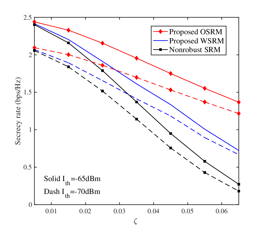
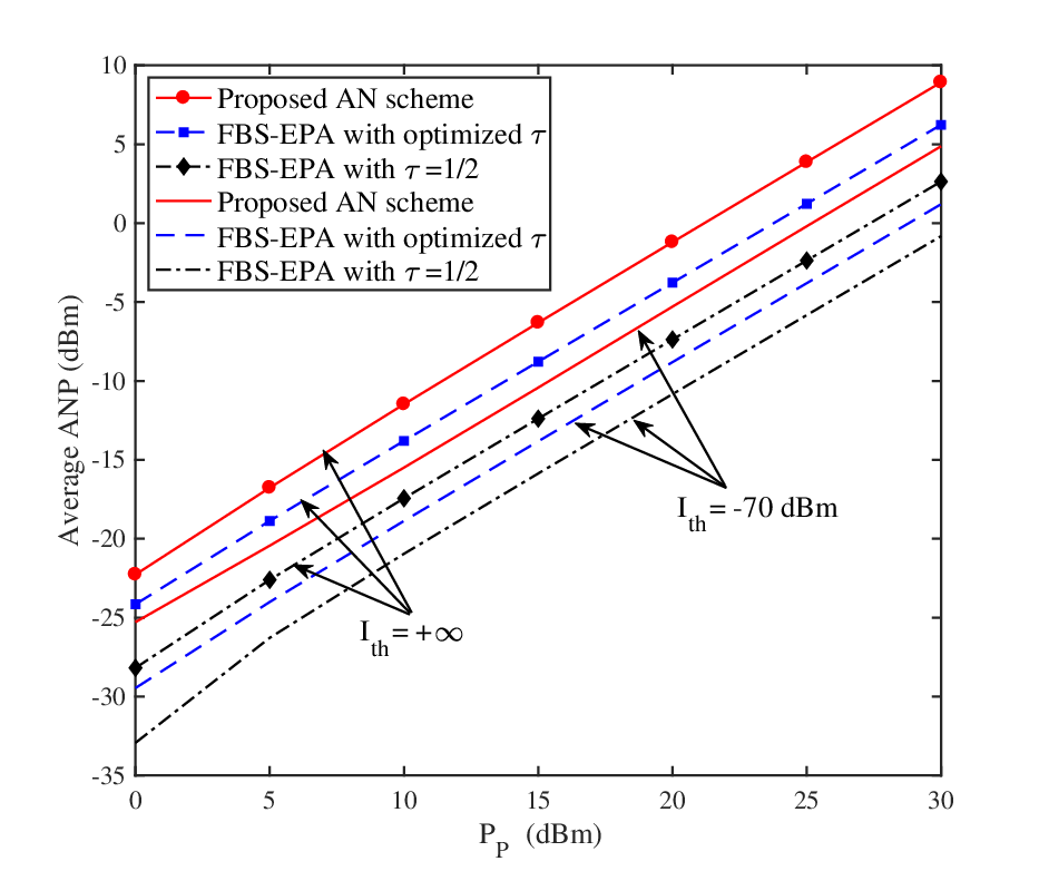
Fig. 6 illustrates secrecy rate performance of all schemes versus the CSI error variance $\zeta$ with different interference levels $I_{th}=-65,-70$ dBm. On the one hand, for each $I_{th}$ , we observe that the achievable secrecy rates of all schemes decrease with the increasing $\zeta$ . The proposed OSRM still has better secrecy rate performance than the proposed WSRM. While the nonrobust SRM performs the worst. Moreover, the performance gaps between the proposed OSRM and the other two schemes both become larger when $\zeta$ increases. On the other hand, the higher secrecy rates of all schemes are observed at the interference level $I_{th}\!=\!-65$ dBm due to the larger feasible region of our secrecy beamforming design.

VI-C The proposed AN scheme

In this subsection, our goal is to illustrate the optimal artificial noise power (ANP) of the proposed AN scheme in Section V. In Fig. 7, the optimized ANP for different schemes versus the PB transmit power $P_{P}$ with different interference thresholds $I_{th}=-70,+\infty$ is shown, where the legitimate rate threshold is set as $R_{th}=1.5$ (bps/Hz). ²² 2 Notice that for some small $P_{P}$ , by which the legitimate rate threshold $R_{th}$ is not supported, we correspondingly set the achievable secrecy rate to be zero. We firstly find from Fig. 7 the achieved ANP increases with $P_{P}$ for all three schemes. Moreover, the proposed AN scheme has the highest ANP compared to the other two schemes, implying that the strongest interference is imposed on the EVE to reduce its wiretapping capability.

Fig. 8 shows the optimal ANP for different schemes versus the legitimate rate threshold $R_{th}$ . It is clear from Fig. 8 that for each scheme, the optimized ANP decreases with the increasing $R_{th}$ since the more portion of PB transmit power $P_{P}$ is allocated for information transfer to the FU for achieving the rate threshold $R_{th}$ . Furthermore, the proposed AN scheme still realizes the highest ANP among all schemes, which promotes secure communications of the wirelessly powered HetNet via sufficiently interfering the malicious Eve.

VII Conclusions

In this paper, we investigated secure communications of the wirelessly powered HetNet from different perspectives of the FBS-EVE CSI. Firstly, in the case of perfect FBS-EVE CSI, the perfect and worst-case SRMs was studied by jointly optimizing the PB energy and FBS information covariance matrices as well as the time splitting factor, which can be globally addressed by the proposed convexity-based linear search. Secondly, considering deterministically and statistically imperfect cases of FBS-EVE CSI, we applied S-procedure and BTI to transform intractable CSI error related constraints into a series of tractable convex ones, respectively. Finally, for the completely unknown FBS-EVE CSI case, an AN aided secrecy beamforming design was proposed to interfere the EVE as much as possible. In particular, when the cross-interference constraint is negligible, the closed-form PB energy covariance matrix for all conisidred cases can be derived. More importantly, we also proved the rank-1 property of the optimal solutions for all studied SRM problems. Numerical experiments verified the excellent secrecy performance of all our proposed secrecy beamforming designs.

Appendix A

Firstly, assuming the fixed $\tau$ and $\eta$ , we can reexpress the relaxed SRM problem (III-A) as

\displaystyle\tilde{R}_{S}^{\star}=\underset{0\leq\tau\leq 1,\eta\geq 1}{\text{max}}\left\{\begin{array}[]{l}\underset{\begin{subarray}{c}\widetilde{\bf W}_{P}\succeq{\bf 0},\widetilde{\bf P}_{F}\succeq{\bf 0}\end{subarray}}{\text{max}}~{C_{1}{\bf h}_{R}^{H}\widetilde{\bf P}_{F}{\bf h}_{R}}\\ ~~~~~{\rm{s.t.}}~~~~~~\widetilde{\text{CR1}}\sim\widetilde{\text{CR4}}\end{array}\right..

Then the proof for Theorem 3 consists of two steps: In the first step, we prove that for any given $\tau$ and $\eta$ , the optimal solution $\{{\widetilde{\bf W}}_{P,1},\widetilde{\bf P}_{F,1}\}$ to the inner maximization problem in (47) is of rank-1. In the second step, we show that $\{{\widetilde{\bf W}}_{P,1},\widetilde{\bf P}_{F,1}\}$ is also optimal to problem (III-A) ( equivalent to the perfect SRM problem (II)), when the same $\tau$ and $\eta$ are adopted. As a result, the equivalence between problem (III-A) and the perfect SRM problem (II) is established.

Step 1: To prove that the optimal solution to the inner maximization problem in (47) is of rank-1, we firstly consider its equivalent counterpart, i.e. the following power minimization problem

\displaystyle\underset{\begin{subarray}{c}\widetilde{\bf W}_{P}\succeq{\bf 0},\widetilde{\bf P}_{F}\succeq{\bf 0}\end{subarray}}{\text{min}}~\text{tr}(\widetilde{\bf P}_{F}),~~~{\rm{s.t.}}~~~\widetilde{\text{CR1}}\sim\widetilde{\text{CR4}};~~\widetilde{\text{PR1}}:C_{1}{\bf h}_{R}^{H}\widetilde{\bf P}_{F}{\bf h}_{R}\geq f_{\eta,\tau}

(46)

where $f_{\eta,\tau}$ denotes the maximum objective value of the inner maximization problem in (47). Clearly, problem (46) is still convex with the linear objective function and convex constraints. In fact, the optimal solution of the inner maximization problem in (47) is the same as that of problem (46), which can be proved by contradiction. Firstly, by assuming that the optimal solution to the inner maximization problem in (47) and problem (46) are $\{\widetilde{\bf W}_{P,1},\widetilde{\bf P}_{F,1}\}$ and $\{\widetilde{\bf W}_{P,2},\widetilde{\bf P}_{F,2}\}$ , respectively, we readily find that $(\widetilde{\bf W}_{P,2},\widetilde{\bf P}_{F,2})$ is feasible for the inner maximization problem in (47) and thus we have ${C_{1}{\bf h}_{R}^{H}\widetilde{\bf P}_{F,2}{\bf h}_{R}}\leq{C_{1}{\bf h}_{R}^{H}\widetilde{\bf P}_{F,1}{\bf h}_{R}}=f_{\eta,\tau}$ . Furthermore, since $(\widetilde{\bf W}_{P,2},\widetilde{\bf P}_{F,2})$ also satisfies $\widetilde{\text{PR1}}$ , it is inferred that $C_{1}{\bf h}_{R}^{H}\widetilde{\bf P}_{F,2}{\bf h}_{R}=f_{\eta,\tau}$ . Clearly, the optimal solution $(\widetilde{\bf W}_{P,2},\widetilde{\bf P}_{F,2})$ to problem (46) is also optimal to the inner maximization problem in (47). In the sequel, we instead investigate the rank-1 property of the optimal solution to problem (46) through Karush-Kuhn-Tucker (KKT) conditions, which are shown in (47) at the top of this page.


		$\displaystyle(1+\beta^{\star}){\bf I}_{N_{F}}+\gamma^{\star}{\bf g}_{P}{\bf g}_{P}^{H}+\rho^{\star}{\bf H}_{E}^{H}{\bf R}_{E}{\bf H}_{E}-\psi^{\star}C_{1}{\bf h}_{R}{\bf h}_{R}^{H}-{\bf Z}_{F}^{\star}={\bf 0}$		(47a)
		$\displaystyle\lambda^{\star}{\bf I}_{N_{P}}+\gamma^{\star}{\bf h}_{M}{\bf h}_{M}^{H}-\beta^{\star}\xi{\bf H}_{F}^{H}{\bf H}_{F}-{\bf Z}_{P}^{\star}={\bf 0}$		(47b)
		$\displaystyle{\bf Z}_{F}^{\star}\widetilde{\bf P}_{F}^{\star}={\bf 0},~{\bf Z}_{P}^{\star}\widetilde{\bf W}_{P}^{\star}={\bf 0}$		(47c)
		$\displaystyle\lambda^{\star}(\text{tr}(\widetilde{\bf W}_{P}^{\star})-\tau P_{P})=0$		(47d)
		$\displaystyle\beta^{\star}(\text{tr}(\widetilde{\bf P}_{F}^{\star})\!-\!\xi\text{tr}({\bf H}_{F}\widetilde{\bf W}_{P}^{\star}{\bf H}_{F}^{H})-\xi\tau\frac{P_{M}}{N_{M}}\text{tr}({\bf G}_{F}{\bf G}_{F}^{H}))=0$		(47e)
		$\displaystyle\gamma^{\star}({\bf h}_{M}^{H}\widetilde{\bf W}_{P}^{\star}{\bf h}_{M}+{\bf g}_{p}^{H}\widetilde{\bf P}_{F}^{\star}{\bf g}_{p}-I_{th})=0$		(47f)
		$\displaystyle\rho^{\star}((1-\eta)(1-\tau)+\text{tr}\big({\bf R}_{E}{\bf H}_{E}\widetilde{\bf P}_{F}^{\star}{\bf H}_{E}^{H}\big))=0$		(47g)
		$\displaystyle\psi^{\star}(C_{1}{\bf h}_{R}^{H}\widetilde{\bf P}_{F}^{\star}{\bf h}_{R}-f_{\eta,\tau})=0$		(47h)

Here, $\{\lambda,\beta,\gamma,\rho,\psi\}$ denote non-negative lagrangian multipliers for constraints $\{\widetilde{\text{CR}}1$ , $\widetilde{\text{CR}}2$ , $\widetilde{\text{CR}}3$ , $\widetilde{\text{CR}}4,\widetilde{\text{PR}}1\}$ in problem (46), respectively. While $\bm{Z}_{P}\succeq\bm{0}$ and $\bm{Z}_{F}\succeq\bm{0}$ are the lagrangian multipliers corresponding to $\widetilde{\bm{W}}_{P}\succeq\bm{0}$ and $\widetilde{\bm{P}}_{F}\succeq\bm{0}$ , respectively. Based on (47a) and (47c), we have $\left((1\!+\!\beta^{\star}){\bf I}_{N_{F}}\!+\!\gamma^{\star}{\bf g}_{P}{\bf g}_{P}^{H}\!+\!\rho^{\star}{\bf H}_{E}^{H}{\bf R}_{E}{\bf H}_{E}\right)\widetilde{\bf P}_{F}^{\star}\!=\!\psi^{\star}C_{1}{\bf h}_{R}{\bf h}_{R}^{H}\widetilde{\bf P}_{F}^{\star},$ implying that

		$\displaystyle\text{rank}\big(\big((1+\beta^{\star}){\bf I}_{N_{F}}+\gamma^{\star}{\bf g}_{P}{\bf g}_{P}^{H}+\rho^{\star}{\bf H}_{E}^{H}{\bf R}_{E}{\bf H}_{E}\big)\widetilde{\bf P}_{F}^{\star}\big)=\text{rank}(\widetilde{\bf P}_{F}^{\star})$
		$\displaystyle=\text{rank}(\psi^{\star}C_{1}{\bf h}_{R}{\bf h}_{R}^{H}\widetilde{\bf P}_{F}^{\star})\leq 1$		(48)

where the first equality in (A) is due to $(1+\beta^{\star}){\bf I}_{N_{F}}+\gamma^{\star}{\bf g}_{P}{\bf g}_{P}^{H}+\rho^{\star}{\bf H}_{E}^{H}{\bf R}_{E}{\bf H}_{E}\succ{\bf 0}$ . According to (A), the rank-1 optimal $\widetilde{\bf P}_{F}^{\star}$ to problem (46) is proved.

As for the optimal $\widetilde{\bf W}_{P}^{\star}$ , we refer to (47b) and (47c) to obtain

\displaystyle\lambda^{\star}{\bf I}_{N_{P}}-\widetilde{\bf H}^{\star}={\bf Z}_{P}^{\star}\succeq{\bf 0},~(\lambda^{\star}{\bf I}_{N_{P}}-\widetilde{\bf H}^{\star})\widetilde{\bf W}_{P}^{\star}={\bf 0},

(49)

where $\widetilde{\bf H}^{\star}=\beta^{\star}\xi{\bf H}_{F}^{H}{\bf H}_{F}-\gamma^{\star}{\bf h}_{M}{\bf h}_{M}^{H}$ . Observing from (49), if $\lambda^{\star}=0$ , then we have $\beta^{\star}\xi{\bf H}_{F}^{H}{\bf H}_{F}\preceq\gamma^{\star}{\bf h}_{M}{\bf h}_{M}^{H}$ , for which $\beta^{\star}=0$ is derived since $\text{rank}(\xi{\bf H}_{F}^{H}{\bf H}_{F})>\text{rank}({\bf h}_{M}{\bf h}_{M}^{H})=1$ is implied by our system setting. The optimal $\widetilde{\bf W}_{P}^{\star}$ is then derived as ${\bf h}_{M}{\bf h}_{M}^{H}\widetilde{\bf W}_{P}^{\star}=0$ . Clearly, there must exist a rank-1 optimal $\widetilde{\bf W}_{P}^{\star}$ in the null space of ${\bf h}_{M}$ . However, if $\lambda^{\star}>0$ , then we have the eigenvalue decomposition (EVD) of $\widetilde{\bf H}^{\star}$ as $\widetilde{\bf H}^{\star}\!\!=\!\!\widetilde{\bf U}_{H}\widetilde{\bf\Lambda}_{H}\widetilde{\bf U}_{H}^{H}$ , where the maximum eigenvalue $\tilde{\lambda}_{{{H}},\max}$ in the diagonal matrix $\widetilde{\bf\Lambda}_{{{H}}}$ must be positive. Otherwise, $\beta^{\star}\xi{\bf H}_{F}^{H}{\bf H}_{F}\preceq\gamma^{\star}{\bf h}_{M}{\bf h}_{M}^{H}$ is implied and only obtained at $\beta^{\star}=0$ as mentioned above. Based on (49), we then have $\widetilde{\bf W}_{P}^{\star}={\bf 0}$ since $\lambda^{\star}>0$ , which contradicts with (47d). So $\lambda^{\star}>0$ yields $\tilde{\lambda}_{{{H}},\max}>0$ and thus we have $\lambda^{\star}{\bf I}_{N_{P}}-\widetilde{\bf H}^{\star}=\widetilde{\bf U}_{H}(\lambda^{\star}{\bf I}_{N_{P}}-\widetilde{\bf\Lambda}_{H})\widetilde{\bf U}_{H}^{H}\succeq{\bf 0}$ . Further, to ensure $\widetilde{\bf W}_{P}^{\star}\neq{\bf 0}$ in (49), it is easily inferred that $\lambda^{\star}=\tilde{\lambda}_{{{H}},\max}$ and thus $\widetilde{\bf W}_{P}^{\star}=c{\bf u}_{P}{\bf u}_{P}^{H}$ is obtained, where ${\bf u}_{P}$ is the unit-norm eigenvector of $\widetilde{\bf H}^{\star}$ corresponding to $\lambda_{{{H}},\max}$ . Moreover, since $\lambda^{\star}=\tilde{\lambda}_{{{H}},\max}>0$ , it yields that $\text{tr}(\widetilde{\bf W}_{P}^{\star})=\tau P_{P}$ and thus $\widetilde{\bf W}_{P}^{\star}=\tau P_{P}{\bf u}_{P}{\bf u}_{P}^{H}$ can be obtained from (47d).

Both cases of $\lambda^{\star}$ demonstrate that the optimal $\widetilde{\bf W}_{P}^{\star}$ to problem (46) is of rank-1. Overall, the rank-1 optimal solution $\{\widetilde{\bf W}_{P},\widetilde{\bf P}_{F}\}$ of the inner maximization problem in (47) is proved.

Step 2: Firstly, we assume that the optimal solution of the inner maximization problem in (47) (equivalent to problem ) and problem (III-A) with the same $\{\eta,\tau\}$ are $\{\widetilde{\bf W}_{P,1},\widetilde{\bf P}_{F,1}\}$ and $\{\widetilde{\bf W}_{P,0},\widetilde{\bf P}_{F,0}\}$ , respectively. The corresponding objective function is defined as $f(\widetilde{\bf W}_{P},\widetilde{\bf P}_{F})$ . Based on Lemma 1, for any given $\eta$ and $\tau$ , the relaxed SRM problem (III-A) actually has a larger feasible solution region than problem (III-A), hence, we have $f(\widetilde{\bf W}_{P,1},\widetilde{\bf P}_{F,1})\geq f(\widetilde{\bf W}_{P,0},\widetilde{\bf P}_{F,0})$ . Furthermore, since both $\widetilde{\bf W}_{P,1},$ and $\widetilde{\bf P}_{F,1}$ are of rank-1 as proved in Step 1, we also find that $\{\widetilde{\bf W}_{P,1},\widetilde{\bf P}_{F,1}\}$ is feasible to problem (III-A), which implies that $f(\widetilde{\bf W}_{P,1},\widetilde{\bf P}_{F,1})\leq f(\widetilde{\bf W}_{P,0},\widetilde{\bf P}_{F,0})$ . Combining the above two inequalities, we finally have $f(\widetilde{\bf W}_{P,1},\widetilde{\bf P}_{F,1})=f(\widetilde{\bf W}_{P,0},\widetilde{\bf P}_{F,0})$ .

Given any $\tau$ and $\eta$ , it is concluded that such a two-tupple $\{{\widetilde{\bf W}}_{P,1},\widetilde{\bf P}_{F,1}\}$ from the relaxed SRM problem (III-A) (inner maximization problem in (47)) is optimal to problem (III-A). Notice that problem (III-A) with the optimal $\tau^{\star}$ and $\eta^{\star}$ is equivalent to the original SRM problem (II), Therefore, the equivalence between problem (III-A) and the PSRM problem (II) is established as that in Theorem 3.

Appendix B

Notice that this proof follows the same logic as that provided for Theorem 3. Firstly, assuming the fixed $\tau$ and $\eta$ , we can reexpress the relaxed robust SRM problem (20) as

\displaystyle\tilde{R}_{S,Ro}^{\star}=\underset{0\leq\tau\leq 1,\eta\geq 1}{\text{max}}\left\{\begin{array}[]{l}\underset{\widetilde{\bf W}_{P}\succeq{\bf 0},\widetilde{\bf P}_{F}\succeq{\bf 0}}{\text{max}}~~{C_{1}{\bf h}_{R}^{H}\widetilde{\bf P}_{F}{\bf h}_{R}}\\ {\rm{s.t.}}~\widetilde{\text{CR1}}\sim\widetilde{\text{CR3}}\\ ~~~~~\widetilde{\text{CR5}}:~\widetilde{\bf I}_{E}-\widetilde{\bf R}_{E}({\bf I}_{N}\otimes\widetilde{\bf P}_{F})\widetilde{\bf R}_{E}^{H}\succeq{\bf 0}\end{array}\right.

where $\widetilde{\bf I}_{E}=\left[\begin{array}[]{cc}u{\bf I}_{N}&{\bf 0}\\ {\bf 0}&\eta-1-\mu\xi_{f}^{2}\end{array}\right]$ and $\widetilde{\bf R}_{E}=\left[\begin{array}[]{c}{\bf R}_{E}^{\frac{1}{2}T}\otimes{\bf I}_{N}\\ \hat{\bf h}_{E}^{H}({\bf R}_{E}^{\frac{1}{2}T}\otimes{\bf I}_{N})\end{array}\right].$ The proof of Theorem 4 is similar to that of Theorem 3 and also consists of the following two steps.

In the first step, we prove that for any given $\tau$ and $\eta$ , the rank-1 optimal solution $\{{\widetilde{\bf W}}_{P},\widetilde{\bf P}_{F}\}$ of the inner maximization problem in (B) is obtained. In the second step, we show that such an $\{{\widetilde{\bf W}}_{P},\widetilde{\bf P}_{F}\}$ is also optimal to the WSRM problem (12). As a result, the equivalence between the relaxed WSRM problem (20) and the original WSRM problem (12) are established.

Similarly, for proving the rank-1 nature of the optimal solution to the inner maximization problem in (B), we consider the corresponding power minimization problem given $\tau$ and $\eta$ as

\displaystyle\underset{\begin{subarray}{c}\widetilde{\bf W}_{P}\succeq{\bf 0},\widetilde{\bf P}_{F}\succeq{\bf 0}\end{subarray}}{\text{min}}~\text{tr}(\widetilde{\bf P}_{F}),~~~{\rm{s.t.}}~~~\widetilde{\text{CR1}}\sim\widetilde{\text{CR3}};~~\widetilde{\text{CR5}};~~\widetilde{\text{PR}}1:C_{1}{\bf h}_{R}^{H}\widetilde{\bf P}_{F}{\bf h}_{R}\geq\hat{f}_{\eta,\tau}.,

(53)

where $\hat{f}_{\eta,\tau}$ denotes the optimal objective value of the inner maximization problem in (B) given any $\tau$ and $\eta$ . It is readily observed that problem (53) is also convex. Following the same philosophy in Step 1 of Appendix A, we readily verify that the optimal solution of problem (53) is also optimal to the inner maximization problem in (B). In the sequel, we aim to show that the optimal solution $\{\widetilde{\bf W}_{P},\widetilde{\bf P}_{F}\}$ of problem (53) for any fixed $\tau$ and $\eta$ are of rank-1 through KKT conditions, which are


		$\displaystyle(1+\beta^{\star}){\bf I}_{N_{F}}+\gamma^{\star}{\bf g}_{P}{\bf g}_{P}^{H}+\rho^{\star}{\bf H}_{E}^{H}{\bf R}_{E}{\bf H}_{E}+\sum\limits_{i=1}^{N_{E}}\widetilde{\bf R}_{E,i}^{H}{\bf Z}_{R}\widetilde{\bf R}_{E,i}-\psi^{\star}C_{1}{\bf h}_{R}{\bf h}_{R}^{H}-{\bf Z}_{F}^{\star}={\bf 0}$		(54a)
		$\displaystyle{\bf Z}_{R}^{\star}(\widetilde{\bf I}_{E}-\widetilde{\bf R}_{E}({\bf I}_{N}\otimes\widetilde{\bf P}_{F})\widetilde{\bf R}_{E}^{H})={\bf 0}$		(54b)
		$\displaystyle\eqref{A2}\sim\eqref{A6},~\eqref{A8}$		(54c)

where $\bm{Z}_{R}\succeq\bm{0}$ is lagrangian multiplier for $\widetilde{\text{CR5}}$ . Based on (54a) and (47c), we have

		$\displaystyle\text{rank}\big(\big((1+\beta^{\star}){\bf I}_{N_{F}}+\gamma^{\star}{\bf g}_{P}{\bf g}_{P}^{H}+\rho^{\star}{\bf H}_{E}^{H}{\bf R}_{E}{\bf H}_{E}+\sum\limits_{i=1}^{N_{E}}\widetilde{\bf R}_{E,i}^{H}{\bf Z}_{R}\widetilde{\bf R}_{E,i}\big)\widetilde{\bf P}_{F}^{\star}\big)=\text{rank}(\widetilde{\bf P}_{F}^{\star})$
		$\displaystyle=\text{rank}(\psi^{\star}C_{1}{\bf h}_{R}{\bf h}_{R}^{H}\widetilde{\bf P}_{F}^{\star})\leq 1.$		(55)

It is clear from (B) that the optimal $\widetilde{\bf P}_{F}^{\star}$ to problem (53) is of rank-1. In addition, since the $\widetilde{\bf W}_{P}$ related KKT conditions of problem (53) are the same as that of problem (46). Let’s refer to Step 1 of Appendix C to prove the rank-1 optimal $\widetilde{\bf W}_{P}^{\star}$ to problem (53). As such, the rank-1 optimal solution $\{\widetilde{\bf P}_{F}^{\star},\widetilde{\bf W}_{P}^{\star}\}$ to problem (53) are finally verified.

Appendix C

According to [30] and following the same argument as Step 1 of Appendix A, the outage-constrained SRM problem (IV-B) given any $\{\tau,{\bf S}\}$ is equivalent to the following power minimization problem

\displaystyle\underset{\begin{subarray}{c}\widetilde{\bf W}_{P}\succeq{\bf 0},\widetilde{\bf P}_{F}\succeq{\bf 0}\end{subarray}}{\text{min}}~~~~~\text{tr}(\widetilde{\bf P}_{F}),~~{\rm{s.t.}}~~\widetilde{\text{CR1}}\sim\widetilde{\text{CR3}},~\widetilde{\text{CR6}}|_{R_{S}=R_{S}^{1}},

(56)

where $R_{S}^{1}$ denotes the optimal objective value of the problem (IV-B) with fixed $\tau$ and ${\bf S}$ . In other words, the optimal solution $\{\widetilde{\bf P}_{F}^{\star},\widetilde{\bf W}_{P}^{\star}\}$ to problem (56) is also optimal to problem (IV-B) given the same $\tau$ and ${\bf S}$ . In the sequel, we firstly prove the rank-1 optimal $\widetilde{\bf P}_{F}^{\star}$ to problem (56). First of all, we define the projection matrix ${\bf T}$ of the vector $\widetilde{\bf P}_{F}^{\frac{1}{2}\star}{\bf h}_{R}$ as ${\bf T}=\frac{\widetilde{\bf P}_{F}^{\frac{1}{2}\star}{\bf h}_{R}{\bf h}_{R}^{H}\widetilde{\bf P}_{F}^{\frac{1}{2}\star}}{\|{\bf h}_{R}^{H}\widetilde{\bf P}_{F}^{\frac{1}{2}\star}\|^{2}}$ , then a novel rank-1 solution $\widehat{\bf P}_{F}^{\star}=\widetilde{\bf P}_{F}^{\frac{1}{2}\star}{\bf T}\widetilde{\bf P}_{F}^{\frac{1}{2}\star}$ is available and satisfies

\displaystyle\text{tr}(\widehat{\bf P}_{F}^{\star})-\text{tr}(\widetilde{\bf P}_{F}^{\star})=\text{tr}(\widetilde{\bf P}_{F}^{\frac{1}{2}\star}({\bf T}-{\bf I})\widetilde{\bf P}_{F}^{\frac{1}{2}\star})\leq 0.

(57)

The formulation (57) yields $\text{tr}(\widehat{\bf P}_{F}^{\star})\leq\text{tr}(\widetilde{\bf P}_{F}^{\star})$ , which hints that the objective value of problem (IV-B) is non-increasing while still satisfying constraints $\widetilde{\text{CR1}}\sim\widetilde{\text{CR2}}$ . Moreover, observing from $\widetilde{\text{CR6}}$ , we have

\displaystyle\log_{2}\big(1+\frac{C_{1}{\bf h}_{R}^{H}\widehat{\bf P}_{F}^{\star}{\bf h}_{R}}{1-\tau}\big)=\log_{2}\bigg(1+\frac{C_{1}|{\bf h}_{R}^{H}\widetilde{\bf P}_{F}^{\star}{\bf h}_{R}|^{2}}{(1-\tau)\|\widetilde{\bf P}_{F}^{\frac{1}{2}\star}{\bf h}_{R}\|^{2}}\bigg)=\log_{2}\big(1+\frac{C_{1}{\bf h}_{R}^{H}\widetilde{\bf P}_{F}^{\star}{\bf h}_{R}}{1-\tau}\bigg)

(58)

as well as

		$\displaystyle\log_{2}\det\bigg({{\bf I}}_{N_{E}}\!+\!\frac{{\bf R}_{E}{\bf H}_{E}\widehat{\bf P}_{F}^{\star}{\bf H}_{E}^{H}}{1-\tau}\bigg)=\log_{2}\bigg({{\bf I}}_{N_{E}}\!+\!\frac{{\bf R}_{E}{\bf H}_{E}\widetilde{\bf P}_{F}^{\frac{1}{2}\star}{\bf T}\widetilde{\bf P}_{F}^{\frac{1}{2}\star}{\bf H}_{E}^{H}}{(1-\tau)}\bigg)$
		$\displaystyle=\log_{2}\bigg(1\!+\!\frac{{\bf h}_{R}^{H}\widetilde{\bf P}_{F}^{\frac{1}{2}\star}(\widetilde{\bf P}_{F}^{\frac{1}{2}\star}{\bf H}_{E}^{H}{\bf R}_{E}{\bf H}_{E}\widetilde{\bf P}_{F}^{\frac{1}{2}\star})\widetilde{\bf P}_{F}^{\frac{1}{2}\star}{\bf h}_{R}}{(1-\tau)\\|{\bf h}_{R}^{H}\widetilde{\bf P}_{F}^{\frac{1}{2}\star}\\|^{2}}\bigg)\leq\log_{2}\big(1\!+\frac{\lambda_{\max}(\widetilde{\bf P}_{F}^{\frac{1}{2}\star}{\bf H}_{E}^{H}{\bf R}_{E}{\bf H}_{E}\widetilde{\bf P}_{F}^{\frac{1}{2}\star})}{1-\tau}\big)$
		$\displaystyle\leq\log_{2}\det({\bf I}_{N_{F}}+\frac{\widetilde{\bf P}_{F}^{\frac{1}{2}\star}{\bf H}_{E}^{H}{\bf R}_{E}{\bf H}_{E}\widetilde{\bf P}_{F}^{\frac{1}{2}\star}}{1-\tau})=\log_{2}\det({\bf I}_{N_{E}}+\frac{{\bf R}_{E}{\bf H}_{E}\widetilde{\bf P}_{F}^{\star}{\bf H}_{E}^{H}}{1-\tau}).$		(59)

Based on (58) and (C), it yields

		$\displaystyle\log_{2}\big(1+\frac{C_{1}{\bf h}_{R}^{H}\widehat{\bf P}_{F}^{\star}{\bf h}_{R}}{1-\tau}\big)-\log_{2}\det\bigg({{\bf I}}_{N_{E}}\!+\!\frac{{\bf R}_{E}{\bf H}_{E}\widehat{\bf P}_{F}^{\star}{\bf H}_{E}^{H}}{1-\tau}\bigg)$
		$\displaystyle\geq\log_{2}\big(1+\frac{C_{1}{\bf h}_{R}^{H}\widetilde{\bf P}_{F}^{\star}{\bf h}_{R}}{1-\tau}\big)-\log_{2}\det\bigg({{\bf I}}_{N_{E}}\!+\!\frac{{\bf R}_{E}{\bf H}_{E}\widetilde{\bf P}_{F}^{\star}{\bf H}_{E}^{H}}{1-\tau}\bigg),$		(60)

which means that the constraint $\widetilde{\text{CR6}}$ still holds by using the novel solution $\widehat{\bf P}_{F}^{\star}$ . Similarly, by referring to (57) and the following inequality

\displaystyle{\bf g}_{p}^{H}\widehat{\bf P}_{F}^{\star}{\bf g}_{p}={\bf g}_{p}^{H}\widetilde{\bf P}_{F}^{\frac{1}{2}\star}{\bf T}\widetilde{\bf P}_{F}^{\frac{1}{2}\star}{\bf g}_{p}=\frac{|{\bf g}_{p}^{H}\widetilde{\bf P}_{F}^{\frac{1}{2}\star}\widetilde{\bf P}_{F}^{\frac{1}{2}\star}{\bf h}_{R}|^{2}}{\|\widetilde{\bf P}_{F}^{\frac{1}{2}\star}{\bf h}_{R}\|^{2}}\leq{\bf g}_{p}^{H}\widetilde{\bf P}_{F}^{\star}{\bf g}_{p},

(61)

the constraint $\widetilde{\text{CR3}}$ can also be satisfied with $\{\widehat{\bf P}_{F}^{\star},\widetilde{\bf W}_{P}^{\star}\}$ . This phenomenon indicates that the novel solution $\{\widehat{\bf P}_{F}^{\star},\widetilde{\bf W}_{P}^{\star}\}$ is also feasible to problem (56) and may even realize a lower objective value than $\{\widetilde{\bf P}_{F}^{\star},\widetilde{\bf W}_{P}^{\star}\}$ . As a result, we conclude that the optimal ${\bf P}_{F}^{\star}$ to problem (56) (equivalent to the outage-constrained SRM problem (IV-B)) must be of rank-1. Since the $\widetilde{\bf W}_{P}$ related KKT conditions of problem (IV-B) are also the same as that of problem (46), the proof for the rank-1 optimal $\widetilde{\bf W}_{P}$ to problem (46) in Appendix A can still be applied to problem (IV-B). Due to space limitation, the detailed proof is omitted here. Overall, the rank-1 optimal solution $\widetilde{\bf P}_{F}^{\star},\widetilde{\bf W}_{P}^{\star}$ to the outage-constrained SRM problem (IV-B) is proved.

Appendix D

Recalling the proof in Step 1 of Appendix A, for any fixed $\tau$ , we readily infer that the AN aided problem (V) is equivalent to the following power minimization problem

		$\displaystyle\underset{\begin{subarray}{c}{\tau},\widetilde{\bf W}_{P}\succeq{\bf 0},\widetilde{\bf P}_{F}\succeq{\bf 0},\widetilde{\bf\Sigma}_{U}\succeq{\bf 0}\end{subarray}}{\text{min}}~~\text{tr}(\widetilde{{\bf P}}_{F})$
		$\displaystyle~~~~~~~~~{\rm{s.t.}}~\widetilde{\text{AR1}}:\text{tr}(\widetilde{\bf\Sigma}_{U})\geq f_{A},~\widetilde{\text{AR2}}:\text{tr}(C_{1}{\bf h}_{R}^{H}\widetilde{\bf P}_{F}{\bf h}_{R})\geq C_{2},~\widetilde{\text{CR1}},~\widetilde{\text{AR3}},~\widetilde{\text{CR3}},$		(62)

where $f_{A}$ denotes the optimal objective value of problem (V) and $C_{2}=(1-\tau)(2^{\frac{R_{th}}{(1-\tau)}}-1)$ . To demonstrate the rank-1 optimal solution $\{\widetilde{\bf W}_{P},\widetilde{\bf P}_{F},\widetilde{\bf\Sigma}_{U}\}$ to problem (D), we formulate the corresponding KKT conditions as


		$\displaystyle(1+\beta^{\star}){\bf I}_{N_{F}}+\gamma^{\star}{\bf g}_{p}{\bf g}_{p}^{H}-\psi^{\star}C_{1}{\bf h}_{R}{\bf h}_{R}^{H}-{\bf Z}_{F}^{\star}={\bf 0},$		(63a)
		$\displaystyle(\beta^{\star}-\rho^{\star}){\bf I}_{N_{F}}+\gamma^{\star}{\bf g}_{p}{\bf g}_{p}^{H}-{\bf Z}_{U}^{\star}={\bf 0},$		(63b)
		$\displaystyle{\bf Z}_{U}^{\star}\widetilde{\bf\Sigma}_{U}^{\star}={\bf 0},~\eqref{A2}\sim\eqref{A6},~\eqref{A8}\|_{f_{\eta,\tau}=C_{2}},$		(63c)

where $\{\rho^{\star},\psi^{\star},\beta^{\star}\}$ , $\lambda^{\star}$ and $\gamma^{\star}$ are the optimal lagrangian multipliers associated with constraints $\widetilde{\text{AR1}}\sim\widetilde{\text{AR3}}$ , $\widetilde{\text{CR1}}$ and $\widetilde{\text{CR3}}$ , respectively, while ${\bf Z}_{U}^{\star}\succeq{\bf 0}$ is the optimal lagrangian multiplier for $\widetilde{\bf\Sigma}_{U}\succeq{\bf 0}$ . It is readily observed from (63a) and (47c) that

\displaystyle\text{rank}\big(\big[(1+\beta^{\star}){\bf I}_{N_{F}}+\gamma^{\star}{\bf g}_{P}{\bf g}_{P}^{H}\big]\widetilde{\bf P}_{F}^{\star}\big)=\text{rank}(\widetilde{\bf P}_{F}^{\star})=\text{rank}(\psi^{\star}C_{1}{\bf h}_{R}{\bf h}_{R}^{H}\widetilde{\bf P}_{F}^{\star})\leq 1,

(64)

which implies that the optimal $\widetilde{\bf P}_{F}^{\star}$ to problem (D) is of rank-1. Additionally, based on (63b) and (63c), we also find that $\beta^{\star}-\rho^{\star}\geq 0$ for guaranteeing ${\bf Z}_{U}^{\star}\succeq{\bf 0}$ . To be specific, when $\beta^{\star}-\rho^{\star}=0$ , we have $\gamma^{\star}{\bf g}_{p}{\bf g}_{p}^{H}\widetilde{\bf\Sigma}_{U}^{\star}={\bf 0}$ . Clearly, there must exist a rank-1 optimal $\widetilde{\bf\Sigma}_{U}^{\star}$ within the null space of ${\bf g}_{p}^{H}$ . While for $\beta^{\star}-\rho^{\star}>0$ , ${\bf Z}_{U}^{\star}\succ{\bf 0}$ and $\widetilde{\bf\Sigma}_{U}^{\star}={\bf 0}$ are obtained according to (63c). Based on above discussion, the rank-1 optimal $\widetilde{\bf\Sigma}_{U}^{\star}$ to problem (D) can be proved. Without loss of generality, the $\widetilde{\bf W}_{P}$ related constraints of problem (D) are also identical to that of problem (46). Therefore, the rank-1 nature of the optimal $\widetilde{\bf W}_{P}^{\star}$ to problem (D) can be verified. Considering the equivalence between problems (D) and (V), we finally conclude that the optimal solution $\{\widetilde{\bf W}_{P},\widetilde{\bf P}_{F},\widetilde{\bf\Sigma}_{U}\}$ of problem (V) is also of rank-1.

Appendix E

Since it has been proved that the globally optimal or high-quality suboptimal FBS information covariance matrices ${\bf P}_{F}$ for all studied problems, namely (II), (12), (23) and (V), are all of rank-1, accordingly, we can define the optimal ${\bf P}_{F}^{\star}=\lambda_{P}{\bf p}_{F}{\bf p}_{F}^{H}$ with $\|{\bf p}_{F}\|_{F}=1$ and $\lambda_{P}>0$ for all these problems. Furthermore, by substituting ${\bf P}_{F}^{\star}=\lambda_{P}{\bf p}_{F}{\bf p}_{F}^{H}$ into the secrecy rate expression in (4), it yields

	$\displaystyle R_{S}$	$\displaystyle=(1-\tau)\log_{2}\big(1+C_{1}\lambda_{P}{{\bf h}_{R}^{H}\bm{p}_{F}\bm{p}_{F}^{H}{\bf h}_{R}}\big)-(1-\tau)\log_{2}\det\big({{\bf I}}_{N_{E}}\!+\!{\bf R}_{E}{\bf H}_{E}{\bf P}_{F}{\bf H}_{E}^{H}\big)$
		$\displaystyle=(1-\tau)\log_{2}\bigg(1+\frac{C_{1}\|{\bf h}_{R}^{H}\bm{p}_{F}\|^{2}-\\|{\bf R}_{E}^{\frac{1}{2}}{\bf H}_{E}{\bf p}_{F}\\|_{F}^{2}}{\frac{1}{\lambda_{P}}+\\|{\bf R}_{E}^{\frac{1}{2}}{\bf H}_{E}{\bf p}_{F}\\|_{F}^{2}}\bigg).$		(65)

Notice that our work aims to optimize $\bm{P}_{F}$ for achieving the maximum non-negative secrecy rate $R_{S}$ , so we must have $C_{1}|{\bf h}_{R}^{H}\bm{p}_{F}|^{2}\geq\|{\bf R}_{E}^{\frac{1}{2}}{\bf H}_{E}{\bf p}_{F}\|_{F}^{2}$ at the optimal ${\bf P}_{F}^{\star}=\lambda_{P}{\bf p}_{F}{\bf p}_{F}^{H}$ . Based on this, it can be found from (E) that $R_{S}$ is a monotonically non-decreasing function of $\lambda_{P}$ . Additionally, when the cross-interference constraint CR3 is inactive for each problem, it is clear that $\lambda_{P}$ is only subject to the constraint CR2 for problems (II), (12), (23), or constraints AR2 and AR3 for problem (V). Based on (E) and problem (V), we readily infer that both CR2 and AR3 are active at the optimal ${\bf P}_{F}^{\star}$ for maximizing secrecy rate $R_{S}$ and artificial noise power, respectively. Inspired by this conclusion, we further formulate the common subproblem for optimizing PB energy covariance matrices ${\bf W}_{P}$ in different cases of FBS-EVE CSI with the inactive CR3 as

\displaystyle\underset{\tau,{\bf W}_{P}\succeq{\bf 0}}{\text{max}}~~~\tau\xi\text{tr}({\bf H}_{F}{\bf W}_{P}{\bf H}_{F}^{H}),~~~{\rm{s.t.}}~~\text{CR1:}~0\leq\tau\leq 1,~\text{tr}({\bf W}_{P})\leq P_{P}.

(66)

According to [31, Lemma H.1.h], we readily derive the closed-form solution ${\bf W}_{P}^{\star}$ to problem (66) as ${\bf W}_{P}^{\star}=P_{P}{{\bf w}_{P}{\bf w}_{P}^{H}}$ with ${\bf w}_{P}=\nu_{\max}({\bf H}_{F}^{H}{\bf H}_{F})$ .

References

[1] M. Shafi et al.,“5G: A tutorial overview of standards, trials, challenges, deployment, and practice,” IEEE J. Select. Areas Commun., vol. 35, no. 6, pp. 1201–1221, Jun. 2017.
[2] F. Boccardi, R. Heath, A. Lozano, T. Marzetta, and P. Popovski, “Five disruptive technology directions for 5G,” IEEE Commun. Mag., vol. 52, no. 2, pp. 74–80, Feb. 2014.
[3] E. Hossain, M. Rasti, H. Tabassum, and A. Abdelnasser, “Evolution toward 5G multi-tier cellular wireless networks: An interference management perspective,” IEEE Wireless Commun., vol. 21, no. 3, pp. 118-127, Jun. 2014.
[4] G. Zhao, S. Chen, L. Zhao and L. Hanzo,“Energy-spectral-efficiency analysis and optimization of heterogeneous cellular networks: A large-scale user-behavior perspective,” IEEE Trans. Veh. Techno., vol. 67, no. 5, pp. 4098-4112, May 2018.
[5] H. S. Jo, Y. J. Sang, P. Xia, and J. G. Andrews, “Heterogeneous cellular networks with flexible cell association: A comprehensive downlink SINR analysis,” IEEE Trans. Wireless Commun., vol. 11, no. 10, pp. 3484–3495, Oct. 2012.
[6] A. Damnjanovic et al.,“A survey on 3GPP heterogeneous networks,” IEEE Wireless Commun., vol. 18, no. 3, pp. 10–21, Jun. 2011.
[7] S. Gong, S. Ma, C. Xing and G. Yang,“Optimal beamforming and time allocation for partially wireless powered sensor networks with downlink SWIPT,” IEEE Trans. Signal Process., vol. 67, no. 12, pp. 3197-3212, Jun. 2019.
[8] J. Hu, K. Yang, G. Wen and L. Hanzo,“Integrated data and energy communication network: A comprehensive survey,” IEEE Commun. Surveys Tuts., vol. 20, no. 4, pp. 3169–3219, Fourthquarter 2018.
[9] R. Zhang, R. G. Maunder and L. Hanzo, “Wireless information and power transfer: from scientific hypothesis to engineering practice,” IEEE Commun. Mag., vol. 53, no. 8, pp. 99-105, Aug. 2015.
[10] H. Tabassum and E. Hossain, “On the deployment of energy sources in wireless-powered cellular networks,” IEEE Trans. Commun., vol. 63, no. 9, pp. 3391–3404, Sept. 2015.
[11] S. Lohani, E. Hossain, and V. K. Bhargava, “On downlink resource allocation for SWIPT in small cells in a two-tier hetnet,” IEEE Trans. Wireless Commun., vol. 15, no. 11, pp. 7709–7724, Nov. 2016.
[12] S. Akbar, Y. Deng, A. Nallanathan, M. Elkashlan, and A. H. Aghvami, “Simultaneous wireless information and power transfer in K-tier heterogeneous cellular networks,” IEEE Trans. Wireless Commun., vol. 15, no. 8, pp. 5804–5818, Aug. 2016.
[13] Y. Zhu, L. Wang, K.-K. Wong, S. Jin, and Z. Zheng, “Wireless power transfer in massive MIMO aided HetNets with user association,” IEEE Trans. Commun., vol. 64, no. 10, pp. 4181–4195, Oct. 2016.
[14] M. Sheng, L. Wang, X. Wang, Y. Zhang, C. Xu, and J. Li, “Energy efficient beamforming in MISO heterogeneous cellular networks with wireless information and power transfer,” IEEE J. Select. Areas Commun., vol. 34, no. 4, pp. 954–968, Apr. 2016.
[15] H. Zhang, S. Huang, C. Jiang, K. Long, V. C. M. Leung, and H. V. Poor, “Energy efficient user association and power allocation in millimeter-wave-based ultra dense networks with energy harvesting base stations,” IEEE J. Select. Areas Commun., vol. 35, no. 9, pp. 1936–1947, Sept. 2017.
[16] J. Kim, H. Lee, C. Song, T. Oh, and I. Lee, “Sum throughput maximization for multi-user MIMO cognitive wireless powered communication networks,” IEEE Trans. Wireless Commun., vol. 16, no. 2, pp. 913–923, Feb. 2017.
[17] T. Lv, H. Gao, and S. Yang, “Secrecy transmit beamforming for heterogeneous networks,” IEEE J. Select. Areas Commun., vol. 33, no. 6, pp. 1154–1170, Jun. 2015.
[18] E. Tekin and A. Yener, “The Gaussian multiple access wire-tap channel,” IEEE Trans. Inform. Theory, vol. 54, no. 12, pp. 5747–5755, Dec. 2008.
[19] Y. S. Shiu, S. Y. Chang, H. C. Wu, S. C. H. Huang, and H. H. Chen, “Physical layer security in wireless networks: A tutorial,” IEEE Wireless Commun., vol. 18, no. 2, pp. 66–74, Apr. 2011.
[20] Y. Ren, T. Lv, H. G. 0001, and Y. Li, “Secure wireless information and power transfer in heterogeneous networks,” IEEE Access, vol. 5, pp. 4967–4979, 2017.
[21] B. Li, Z. Fei, Z. Chu, and Y. Zhang, “Secure transmission for heterogeneous cellular networks with wireless information and power transfer,” IEEE Systems Journal, vol. 12, no. 4, pp. 3755–3766, Dec. 2018.
[22] X. Hu, Li, K. Huang, Z. Fei, and K. K. Wong, “Secrecy energy efficiency in wireless powered heterogeneous networks: A distributed ADMM approach,” IEEE Access, vol. 6, pp. 20609-20624, 2018.
[23] D. W. K. Ng, E. S. Lo, and R. Schober, “Multiobjective resource allocation for secure communication in cognitive radio networks with wireless information and power transfer,” IEEE Trans. Veh. Techno., vol. 65, no. 5, pp. 3166–3184, May 2016.
[24] Y. Yuan and Z. Ding, “Outage constrained secrecy rate maximization design with SWIPT in MIMO-CR systems,” IEEE Trans. Veh. Techno., vol. 67, no. 6, pp. 5475–5480, Jun. 2018.
[25] Y. Wu, X. Chen, C. Yuen, and C. Zhong, “Robust resource allocation for secrecy wireless powered communication networks,” IEEE Commun. Letters, vol. 20, no. 12, pp. 2430–2433, Dec. 2016.
[26] Q. Li and W. K. Ma, “Optimal and robust transmit designs for MISO channel secrecy by semidefinite programming,” IEEE Trans. Signal Process., vol. 59, no. 8, pp. 3799–3812, Aug. 2011.
[27] S. Boyd and L. Vandenberghe, Convex Optimization. Cambridge, U.K.: Cambridge Univ. Press, 2004.
[28] Z. Q. Luo, J. F. Sturm, and S. Z. Zhang, “Multivariate nonnegative quadratic mappings,” SIAM J. Optim., vol. 14, no. 4, pp. 1140–1162, 2004.
[29] S. S. Christensen, R. Agarwal, E. de Carvalho, and J. M. Cioffi, “Weighted sum-rate maximization using weighted MMSE for MIMO-BC beamforming design,” IEEE Trans. Wireless Commun., vol. 7, no. 12, pp. 4792–4799, 2008.
[30] S. Ma, M. Hong, E. Song, X. Wang, and D. Sun, “Outage constrained robust secure transmission for MISO wiretap channels,” IEEE Trans. Wireless Commun., vol. 13, no. 10, pp. 5558–5570, Oct. 2014.
[31] A. Marshall and I. Olkin, Inequalities: theory of majorization and its applications. Academic Press New York, 1979.