A Nonlinear Hyperbolic Model for Radiative Transfer Equation in Slab Geometry

Yuwei Fan Thanks: Department of Mathematics, Stanford University, Stanford, CA 94305, email: ywfan@stanford.edu Ruo Li Thanks: HEDPS & CAPT, LMAM & School of Mathematical Sciences, Peking University, Beijing, China, email: rli@math.pku.edu.cn and Lingchao Zheng Thanks: School of Mathematical Sciences, Peking University, Beijing, China, email: lczheng@pku.edu.cn

Abstract

Linear models for the radiative transfer equation have been well developed, while nonlinear models are seldom investigated even for slab geometry due to some essential difficulties. We have proposed a moment model in [24] for slab geometry, which combines the ideas of the classical $P_{N}$ and $M_{N}$ model. Though the model is far from perfect, it was demonstrated to be quite efficient in numerically approximating the solution of the radiative transfer equation, that we are motivated to improve this model further. Consequently, we propose in this paper a new model following the chartmap in [24] with some significant theoretic progresses. The new model is derived with global hyperbolicity, and meanwhile some necessary physical properties are preserved. We give a complete analysis of the characteristic structure and propose a numerical scheme for the new model. Numerical examples are presented to demonstrate the numerical performance of the new model.

Keywords: Radiative transfer equation; slab geometry; nonlinear model; global hyperbolicity.

1 Introduction

In kinetic theory, the radiative transfer equation (RTE), which is the evolution equation of the specific intensity, describes the motion of photons and their interaction with the background medium. In the past decades, it has many applications in different fields, for instance, radiation astronomy [43], reactor physics [46, 21], atmospheric radiative transfer [38], and optical imaging [32, 51]. The RTE is a high-dimensional integro-differential kinetic equation, so how to develop effective numerical methods for RTE is an important issue. The common numerical methods can be classified into two categories: the probabilistic methods like the direct simulation Monte Carlo (DSMC) methods [3, 29, 18], and the deterministic schemes [4, 36, 48, 31, 17, 20, 44, 2, 22, 24], such as the discrete ordinates method ( $S_{N}$ ) [4, 36, 48], the moment methods [31, 17, 20, 2, 24] and etc.

The DSMC method, introduced by Bird in [3], follows a representative set of photons as they interact with background and move in physical space. So far, this method has made remarkable successes in solving the RTE, but the statistical scatter (or statistical noise) is the main issue for its accuracy. In order to improve accuracy, one needs to increase the number of photons, which significantly increases both the computational and memory requirements.

The discrete ordinates method ( $S_{N}$ ), which is one of the most popular deterministic methods, solves the transport equation along with a discrete set of angular directions from a given quadrature set. However, the $S_{N}$ model is based on the assumption that the particles can only move along the directions in the quadrature set, which results in numerical artifacts, known as ray effects [36].

The moment method studies the evolution of a finite number of moments of the specific intensity. Typically, the evolution equation of a lower order moment depends on higher order moments. Hence one has to introduce the called moment closure to close the moment model. A common method for the moment closure is to construct an ansatz to approximate the specific intensity and the two most popular moment methods are the spherical harmonics method ( $P_{N}$ ) [46] and the maximum entropy method ( $M_{N}$ ) [37, 20, 44]. The $P_{N}$ model constructs the ansatz by expanding the specific intensity around the equilibrium in terms of spherical harmonics in the velocity direction. However, the resulting model may lead to nonphysical oscillations, or even worse, negative particle concentration [6, 7, 42]. The $M_{N}$ model constructs the ansatz based on the principle of maximum entropy [37, 20]. However, no algebraic expression of the moment closure is known for the case $N\geq 2$ , and one has to solve an ill-conditioned optimization problem to obtain the moment closure in the implementation, which strongly limits the application of the $M_{N}$ model.

Recently, a nonlinear moment model (called the ${M\!P}_{\!N}$ model) was proposed in [24]. This model takes the ansatz of the $M_{1}$ model (the first order of the $M_{N}$ model) as the weight function, then constructs the ansatz by expanding the specific intensity around the weight function in terms of orthogonal polynomials in the velocity direction. The ${M\!P}_{\!N}$ model is a nonlinear model since the weight function contains the energy flux of the intensity. Numerical tests in [24] demonstrate its numerical efficiency and show that the ${M\!P}_{\!N}$ model produces an improved approximation of the intensity in comparison of the $P_{N}$ model in [24]. Moreover, it was proved that the ${M\!P}_{\!N}$ model with $N=2$ is globally hyperbolic in the realizable domain.

In spite of its numerous progress, the ${M\!P}_{\!N}$ model is, however, far from perfect. The theoretical investigation shows that the ${M\!P}_{\!N}$ model with $N\geq 3$ loses its hyperbolicity when the specific intensity is far away from the equilibrium. For the case $N=2$ , the ${M\!P}_{\!N}$ model might give unphysical characteristic speeds. Precisely, the characteristic speeds could be faster than the speed of light. Detailed discussion is presented in section 2.3. These defects limit the application of the ${M\!P}_{\!N}$ model on the strong non-equilibrium problems and time-dependent problems. Encouraged by the improved numerical performance of the ${M\!P}_{\!N}$ model, we are motivated to study further following this spirit to get rid of these limits. The top object is to study how to gain hyperbolicity of the ${M\!P}_{\!N}$ model.

Although the hyperbolicity is a critical issue for the moment model, there are not too many works on the hyperbolic regularization till now. The well-known entropy-based $M_{N}$ model [37] is globally hyperbolic because its ansatz is an exponential function, which makes the model symmetric hyperbolic. However, it does not provide clues for other models to gain hyperbolicity. The first globally hyperbolic regularization was proposed in [8, 9], where the authors study the regularization by investigating the coefficient matrix of the reduced model. This work was extended to a general framework on deriving a hyperbolic reduced model for generic kinetic equations in [10, 23] based on the operator projection (or truncation). Many follow-up works were proposed after that, for instance [11, 12, 34, 19, 35]. We refer readers to [33] and references therein for more details. Hence, a natural idea is to apply the hyperbolic regularization framework in [10, 23] on the ${M\!P}_{\!N}$ model to yield a globally hyperbolic model. However, though being hyperbolic, the resulting model is not satisfied since it changes the model even for $N=1$ , in which case the ${M\!P}_{\!N}$ model is precisely the $M_{1}$ model. This indicates the resulting model may not able to yield a correct high-order Eddington approximation. We are obliged to develop additional techniques to attain a satisfied model.

In this paper, we first discuss some natural criteria to improve the ${M\!P}_{\!N}$ model by hyperbolic regularization:

1.

the regularized model is globally hyperbolic;
2.

the characteristic speeds of the regularized model cannot be faster than the speed of light;
3.

the regularization vanishes for the case $N=1$ ;
4.

only the evolution equations that are closed by the moment closure can be changed.

The first criterion is our goal, and the second one is a natural physical constraint. The third one is to guarantee the correctness of the high-order Eddington approximation, and the last one is to attain high efficiency. More discussion is presented in 1, 2, 3 and 4.

Taking these criteria into account, we notice that the key idea of the framework in [10, 23] is that in the convection term, the spatial derivative operator $\dfrac{\partial{\cdot}}{\partial{z}}$ and the multiplying velocity operator $\mu\cdot$ are not coupled in the space defined by the specific intensity but they are coupled in the linear space defined by the ansatz, and then the authors decoupled these two operators to gain the hyperbolicity. Keeping such an idea in mind, we are inspired to propose a modified hyperbolic regularization. Making use of the weight function and the ansatz of the ${M\!P}_{\!N}$ model, we introduce a new space that is defined by the derivative of the weight function with respect to the parameter in the weight function. This makes us decouple the spatial derivative operator and the multiplying velocity operator in this new space. Consequently, the resulting moment model satisfies all the criteria, saying that the new model is not only globally hyperbolic but also retains some physical properties of the RTE. The characteristic structure of the new model is well studied. Moreover, the new hyperbolic regularization generalizes the framework in [10, 23], extends its application range and also takes properties of the kinetic equation into account of the regularization.

To develop a numerical scheme for the new model, we adopt the DLM theory [39] to deal with the non-conservative part by introducing a generalized Rankine-Hugoniot condition. Then the numerical scheme in [47], which can be treated as a non-conservative version of the HLL, is applied to discretize the non-conservative system. Numerical simulations are performed to demonstrate the numerical efficiency of the new model. Thanks to the hyperbolic regularization, the new model works well for the case the ${M\!P}_{\!N}$ model fails. The simulations on benchmark problems show that the new model has good agreement with the reference solution.

The rest of this paper is arranged as follows. Section 2 briefly introduces the RTE and the ${M\!P}_{\!N}$ model. Particularly, we try to discuss the defects of the ${M\!P}_{\!N}$ model in detail to clarify the improvements in the new model. In section 3, we point out the failure of the hyperbolic regularization framework in [10, 23] and propose the generalized hyperbolic regularization method for the ${M\!P}_{\!N}$ model to yield the new model. Numerical scheme and numerical results for the new model are presented in section 4. The paper ends with a conclusion in section 5.

2 ${M\!P}_{\!N}$ Model for Radiative Transfer Equation

The time-dependent radiative transfer equation (RTE) for a grey medium in the slab geometry has the form

\frac{1}{c}\dfrac{\partial{I}}{\partial{t}}+\mu\dfrac{\partial{I}}{\partial{z}}={\mathcal{S}}(I),

(2.1)

where $I=I(z,t,\mu)$ is the specific intensity of radiation and $c$ is the speed of light. The variable $\mu\in[-1,1]$ is the cosine of the angle between the photon velocity and the positive $z$ -axis. The right hand side ${\mathcal{S}}(I)$ denotes the actions by the background medium on the photons, and it usually contains a scattering term, an absorption term, and an emission term.

2.1 Moment method

Denote the $k$ -th moment of the specific intensity by

{\langle I\rangle}_{k}\triangleq\int_{-1}^{1}\mu^{k}I(\mu)\,\mathrm{d}\mu,\quad k\in\mathbb{N},

(2.2)

then multiplying (2.1) by $\mu^{k}$ and integrating it with respect to $\mu$ over $[-1,1]$ yields the moment equations

\frac{1}{c}\dfrac{\partial{{\langle I\rangle}_{k}}}{\partial{t}}+\dfrac{\partial{{\langle I\rangle}_{k+1}}}{\partial{z}}={\langle{\mathcal{S}}(I)\rangle}_{k},\quad k\in\mathbb{N}.

(2.3)

Notice that the governing equation of ${\langle I\rangle}_{k}$ depends on the $(k+1)$ -th moment ${\langle I\rangle}_{k+1}$ , which indicates that the full system contains infinite number of equations. Thus, in order to derive a reduced model for (2.1), we choose a positive integer $N$ and discard all the governing equation of ${\langle I\rangle}_{k}$ , $k>N$ . Clearly, the truncated system is not closed due to its dependence on ${\langle I\rangle}_{N+1}$ , so we need to provide a so-called moment closure for the model. A common strategy of the moment closure is to construct an ansatz for the specific intensity. Precisely, let $E_{k}$ , $k=0,\dots,N$ , be the $k$ -th known moments for a certain unknown specific intensity $I$ . One can propose an approximation, also called ansatz, $\hat{I}(E_{0},\dots,E_{N};\mu)$ such that

{\langle\hat{I}(E_{0},\dots,E_{N};\cdot)\rangle}_{k}=E_{k},\quad k=0,\dots,N,

(2.4)

and $\hat{I}$ is uniquely determined by (2.4). Then the moment closure is given by

E_{N+1}={\langle\hat{I}(E_{0},\dots,E_{N};\cdot)\rangle}_{N+1},

(2.5)

and the moment model is proposed to be the system

\frac{1}{c}\dfrac{\partial{E_{k}}}{\partial{t}}+\dfrac{\partial{E_{k+1}}}{\partial{z}}={\langle{\mathcal{S}}(\hat{I}(E_{0},\dots,E_{N};\mu))\rangle}_{k},\quad k=0,\dots,N.

(2.6)

Based on the moment closure strategy, many existing models are developed in the literature, for example, the $P_{N}$ model [31], the $M_{N}$ model [37, 20], the positive $P_{N}$ model [26], the $B_{2}$ model [2], and the ${M\!P}_{\!N}$ model [24]. The ${M\!P}_{\!N}$ model proposed in [24] shows good numerical results for some standard benchmarks. In this paper, we will restudy this model and point out its defects in both theoretical analysis and limitation on numerical simulations, and then propose a novel regularization for this model.

2.2 ${M\!P}_{\!N}$ model

The ${M\!P}_{\!N}$ model starts from introducing the weight function

\omega^{[\alpha]}(\mu)=\frac{1}{(1+\alpha\mu)^{4}},\quad\alpha\in(-1,1).

(2.7)

Using the Gram-Schmidt orthogonalization, one can directly define a series of monic orthogonal polynomials in the interval $[-1,1]$ with respect to the weight function $\omega^{[\alpha]}(\mu)$ recursively as

\displaystyle\phi^{[\alpha]}_{0}(\mu)=1,\quad\phi^{[\alpha]}_{j}(\mu)=\mu^{j}-\sum_{k=0}^{j-1}\frac{{\mathcal{K}}_{j,k}}{{\mathcal{K}}_{k,k}}\phi^{[\alpha]}_{k}(\mu),\quad j\geq 1,

(2.8)

where the coefficients ${\mathcal{K}}_{j,k}$ is given by

\displaystyle{\mathcal{K}}_{j,k}=\int_{-1}^{1}\mu^{j}\phi^{[\alpha]}_{k}(\mu)\omega^{[\alpha]}(\mu)\,\mathrm{d}\mu.

(2.9)

The orthogonality of $\phi^{[\alpha]}_{k}$ yields

{\mathcal{K}}_{j,k}=0,\text{ if }j<k,\quad{\mathcal{K}}_{k,k}=\int_{-1}^{1}(\phi^{[\alpha]}_{k}(\mu))^{2}\omega^{[\alpha]}\,\mathrm{d}\mu>0.

(2.10)

The ansatz of the ${M\!P}_{\!N}$ model is defined as

\hat{I}(E_{0},\dots,E_{N};\mu)\triangleq\sum_{i=0}^{N}f_{i}\Phi^{[\alpha]}_{i}(\mu),

(2.11)

where $\Phi^{[\alpha]}_{i}(\mu)=\phi^{[\alpha]}_{i}(\mu)\omega^{[\alpha]}(\mu),i=0,1,\dots,N$ are the basis functions, and $f_{i}$ are the expansion coefficients to be determined by the moment constraints (2.4). Thanks to the orthogonality of $\phi^{[\alpha]}_{i}$ , we have

f_{i}=\frac{1}{{\mathcal{K}}_{i,i}}\int_{-1}^{1}\phi^{[\alpha]}_{i}(\mu)\hat{I}(\mu)\,\mathrm{d}\mu,\quad i=0,\dots,N.

Substituting the recursive relationship (2.8) into the upper equation yields the following recursive formulation for $f_{i}$ , which are functions dependent on $E_{i}$ ,

f_{i}=\frac{1}{{\mathcal{K}}_{i,i}}\left(E_{i}-\sum_{j=0}^{i-1}{\mathcal{K}}_{i,j}f_{j}\right),\quad 0\leq i\leq N.

(2.12)

The moment closure is then given by

E_{N+1}=\sum_{k=0}^{N}{\mathcal{K}}_{N+1,k}f_{k}.

(2.13)

For the ${M\!P}_{\!N}$ model, the parameter $\alpha$ is set as $\alpha=-\frac{3E_{1}/E_{0}}{2+\sqrt{4-3(E_{1}/E_{0})^{2}}}$ . In this case, direct calculations yield

f_{1}=0.

(2.14)

2.3 Defects of the ${M\!P}_{\!N}$ model

The ${M\!P}_{\!N}$ model has been well studied in [24]. It was shown that the ansatz (2.11) had a better approximation to the specific intensity than the $P_{N}$ model, and the ${M\!P}_{\!N}$ model was numerically demonstrated to be effective in approximating the RTE. As a particular case, the ${M\!P}_{2}$ model was well studied, including its hyperbolicity and characteristic field for the Riemann problem. Nevertheless, the ${M\!P}_{\!N}$ model is far from perfect, and it has some defects in the theoretical analysis, which limits its application in numerical simulations.

There are a lot of criteria to judge a reduced model. Among them, the following criteria are basic conditions for a physical model:

Criterion 1.

The reduced model is globally hyperbolic.

Criterion 2.

The characteristic speeds of the reduced model lie in $[-c,c]$ .

The 1 uses the following definition.

Definition 1 (Global hyperbolicity).

A system of first order quasi-linear partial differential equations

\dfrac{\partial{\boldsymbol{w}}}{\partial{t}}+{\bf A}(\boldsymbol{w})\dfrac{\partial{\boldsymbol{w}}}{\partial{z}}=0,\quad\boldsymbol{w}\in\Omega

is called hyperbolic at the point $\boldsymbol{w}_{0}\in\Omega$ if the matrix ${\bf A}(\boldsymbol{w}_{0})$ is diagonalizable with real eigenvalues. The system is called globally hyperbolic if it is hyperbolic at each point $\boldsymbol{w}\in\Omega$ .

Since the left hand side of the RTE (2.1) is an advection part, the 1 is the necessary condition for the existence of the solution. Thus, the hyperbolicity is a critical mathematical constraint on the reduced model. The 2 is a basic physical property of the reduced model, which can be interpreted as that the information can not travel faster than the speed of light. However, as will be shown, the ${M\!P}_{\!N}$ model fails to satisfy these criteria.

2.3.1 Loss of global hyperbolicity

In [24], the ${M\!P}_{2}$ model was proved to be globally hyperbolic in its realizability domain. However, the global hyperbolicity fails to be preserved by the ${M\!P}_{\!N}$ model with $N>2$ . In the following, we take the ${M\!P}_{3}$ model as an example to show that the ${M\!P}_{\!N}$ model fails to satisfy the 1.

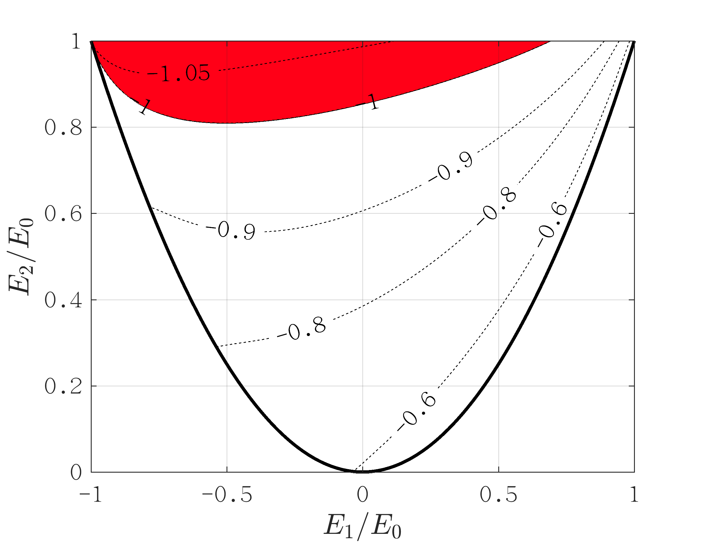
Denote the characteristic polynomial of the ${M\!P}_{3}$ model as $p_{3}(\lambda)$ , then it depends on $E_{k}/E_{0}$ , $k=1,2,3$ , i.e., $p_{3}(\lambda)=p_{3}(E_{1}/E_{0},E_{2}/E_{0},E_{3}/E_{0};\lambda)$ . That all the zeros of $p_{3}(\lambda)$ are real is a necessary condition for the hyperbolicity. Figure 1 plots the real region (the region that all the zeros of $p_{3}(\lambda)$ are real) of $p_{3}(\lambda)$ with some given $E_{3}/E_{0}$ . Clearly, the zeros of $p_{3}(\lambda)$ are not always real; thus the ${M\!P}_{3}$ model is not globally hyperbolic.

2.3.2 Unphysical characteristic speed

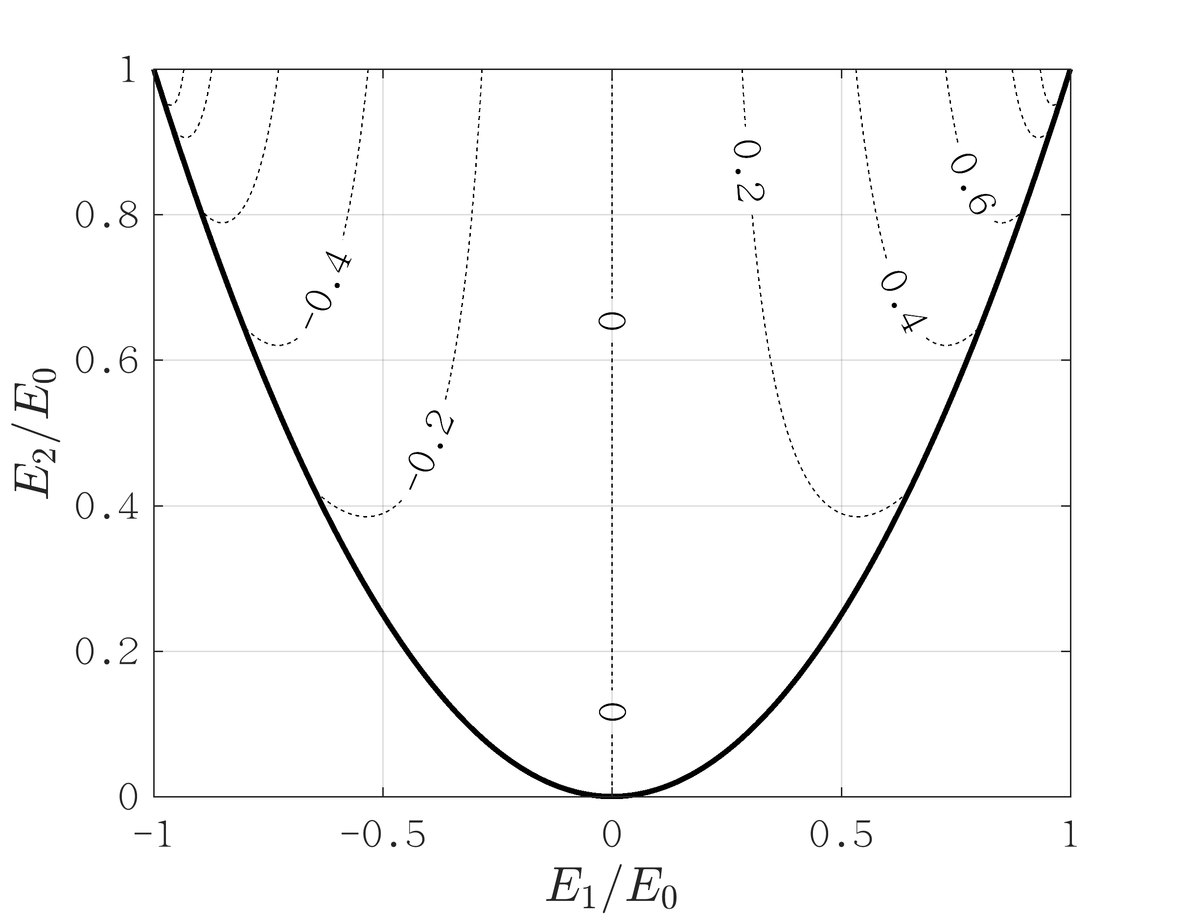
We take the ${M\!P}_{2}$ model as an example to show that the ${M\!P}_{\!N}$ model fails to satisfy the 2. Denote the characteristic polynomial of the ${M\!P}_{2}$ model by $p_{2}(\lambda)$ . Since the ${M\!P}_{2}$ model is strictly hyperbolic [24], all the zeros of $p_{2}(\lambda)$ are real and distinct. We denote the zeros of $p_{2}(\lambda)$ by $\lambda_{k}$ , $k=1,2,3$ with $\lambda_{1}<\lambda_{2}<\lambda_{3}$ . Clearly, the characteristic speeds $\lambda_{k}$ are determined by $E_{1}/E_{0}$ and $E_{2}/E_{0}$ , i.e., $\lambda_{k}=\lambda_{k}(E_{1}/E_{0},E_{2}/E_{0})$ . Figure 2 presents the profile of $\lambda_{k}$ . One can observe that there is a region for $\lambda_{1}$ and $\lambda_{3}$ where the characteristic speed does not lie in $[-c,c]$ .

3 Hyperbolic Regularization

In section 2.3, it is pointed out that the ${M\!P}_{\!N}$ model is not globally hyperbolic and its characteristic speeds can be faster than the speed of light. This motivates us to explore a regularization for the ${M\!P}_{\!N}$ model to eliminate such defects. As is discussed in the introduction, even though the hyperbolicity is a critical property for the reduced model, only a few works on the hyperbolic regularization are proposed. The candidate is the moment model reduction method in [10, 23], which provides a general framework on deriving hyperbolic reduced models from kinetic equations.

On the other hand, one must follow some criteria in the regularization. As is discussed in [24], when $N=1$ , the ${M\!P}_{\!N}$ model is the classical $M_{1}$ model, which satisfies the 1 and 2. It is nature to require that the regularization does not change the ${M\!P}_{1}$ model, i.e.,

Criterion 3.

The regularization vanishes for the case $N=1$ .

Remark 1.

Basically, we should require that the local linearization of the regularized reduced model around the weight function is the same as that of the ${M\!P}_{\!N}$ model. Precisely, we assume $\hat{I}=\omega^{[\alpha]}+\epsilon g$ , where $\epsilon$ is a small quantity, then we use this decomposition to linearize the ${M\!P}_{\!N}$ model and the regularized reduced model by discarding high order terms. The resulting two models should be the same. This constraint is a critical condition for the regularization. Otherwise, even $\hat{I}-\omega^{[\alpha]}$ is quite small, the solution of the ${M\!P}_{\!N}$ model and the regularized reduced model can be qualitatively different. Moreover, if one applies the Chapman-Enskog expansion [16] on the regularized reduced model with $N=2$ to derive the high-order Eddington approximation, the resulting approximation may be not correct (Ref. [19] presents an example for the quantum gas). Although the 3 is a necessary but not sufficient condition for such constraint, this criterion is easy to check and is enough for verifying the regularization in this paper.

In the derivation of the reduced model (2.6), the governing equation of $E_{N}$ is the only unclosed equation. Thus it is the only equation one can modify in the regularization. Precisely, we have the following criterion.

Criterion 4.

To regularize the reduced model (2.6), the governing equation of $E_{k}$ , $k=0,\dots,N-1$ can not be changed.

In this section, we first show that the regularization framework in [10, 23] to regularize the ${M\!P}_{\!N}$ model to be globally hyperbolic can not fulfill all the constraints of 1, 2, 3 and 4. This investigation inspires us to propose a novel regularization by using the special structure of the weight function and the RTE. Then the novel regularization is proposed, and the regularized reduced model is well studied.

3.1 Hyperbolic regularization framework

We first try to apply the regularization framework in [10, 23] on the ${M\!P}_{\!N}$ model and show that the resulting model dissatisfies the 1, 2, 3 and 4. It indicates that a globally hyperbolic regularization on the ${M\!P}_{\!N}$ model is not trivial.

3.1.1 Reformulation of reduced model

In order to apply the regularization framework in [10, 23], we introduce some notations and reformulate the reduced model. Denote $\mathbb{H}$ by the space of all the admissible specific intensity for the RTE and define the Hilbert space

\mathbb{H}^{[\alpha]}_{N}:=\mathrm{span}\left\{\Phi^{[\alpha]}_{i},i=0,\dots,N\right\}

(3.1)

with the inner product

\left\langle{\Phi},{\Psi}\right\rangle_{\mathbb{H}^{[\alpha]}_{N}}=\int_{-1}^{1}\Phi(\mu)\Psi(\mu)/\omega^{[\alpha]}(\mu)\,\mathrm{d}\mu.

(3.2)

Then for each intensity $I\in\mathbb{H}$ , the corresponding ansatz $\hat{I}$ (2.11) for the ${M\!P}_{\!N}$ model is in the space $\mathbb{H}^{[\alpha]}_{N}$ . We define a projection from the space $\mathbb{H}$ to the space $\mathbb{H}^{[\alpha]}_{N}$ as

\displaystyle\mathcal{P}:I

\displaystyle\rightarrow\hat{I}=\sum_{i=0}^{N}f_{i}\Phi^{[\alpha]}_{i},\quad f_{i}=\frac{\left\langle{I},{\Phi^{[\alpha]}_{i}}\right\rangle_{\mathbb{H}^{[\alpha]}_{N}}}{\left\langle{\Phi^{[\alpha]}_{i}},{\Phi^{[\alpha]}_{i}}\right\rangle_{\mathbb{H}^{[\alpha]}_{N}}}=\frac{\int_{-1}^{1}I\phi^{[\alpha]}_{i}\,\mathrm{d}\mu}{{\mathcal{K}}_{i,i}},

(3.3)

where ${\mathcal{K}}_{i,i}$ is defined in (2.8). Since the basis function is the product of the weight function and the orthogonal polynomial, the projection $\mathcal{P}$ is an orthogonal projection.

With the upper notations, the reduced model (2.6) can be equivalently expressed as

\left\langle{\mu^{k}\omega^{[\alpha]}},{\frac{1}{c}\dfrac{\partial{\mathcal{P}I}}{\partial{t}}+\mu\dfrac{\partial{\mathcal{P}I}}{\partial{z}}}\right\rangle_{\mathbb{H}^{[\alpha]}_{N}}=\left\langle{\mu^{k}\omega^{[\alpha]}},{{\mathcal{S}}(\mathcal{P}I)}\right\rangle_{\mathbb{H}^{[\alpha]}_{N}},\quad k=0,\dots,N.

(3.4)

Since the projection $\mathcal{P}$ is an orthogonal projection, we have

\left\langle{\mu^{k}\omega^{[\alpha]}},{\frac{1}{c}\mathcal{P}\dfrac{\partial{\mathcal{P}I}}{\partial{t}}+\mathcal{P}\mu\dfrac{\partial{\mathcal{P}I}}{\partial{z}}}\right\rangle_{\mathbb{H}^{[\alpha]}_{N}}=\left\langle{\mu^{k}\omega^{[\alpha]}},{\mathcal{P}{\mathcal{S}}(\mathcal{P}I)}\right\rangle_{\mathbb{H}^{[\alpha]}_{N}},\quad k=0,\dots,N.

(3.5)

For the simplicity of notations, we write the ${M\!P}_{\!N}$ model (3.5) formally as

\frac{1}{c}\mathcal{P}\dfrac{\partial{\mathcal{P}I}}{\partial{t}}+\mathcal{P}\mu\dfrac{\partial{\mathcal{P}I}}{\partial{z}}=\mathcal{P}{\mathcal{S}}(\mathcal{P}I).

(3.6)

Moreover, noticing that $\{\mu^{k}\omega^{[\alpha]},k=0,\dots,N\}$ and $\{\Phi^{[\alpha]}_{k},k=0,\dots,N\}$ are two sets of basis function of $\mathbb{H}^{[\alpha]}$ , we can also rewrite the reduced model (3.5) equivalently as

\left\langle{\Phi^{[\alpha]}_{k}},{\frac{1}{c}\dfrac{\partial{\mathcal{P}I}}{\partial{t}}+\mu\dfrac{\partial{\mathcal{P}I}}{\partial{z}}}\right\rangle_{\mathbb{H}^{[\alpha]}_{N}}=\left\langle{\Phi^{[\alpha]}_{k}},{{\mathcal{S}}(\mathcal{P}I)}\right\rangle_{\mathbb{H}^{[\alpha]}_{N}},\quad k=0,\dots,N.

(3.7)

We note that all of (3.4), (3.6) and (3.7) are different forms of a same model. The form (3.6) is an abbreviation of (3.5) and is convenient to investigate the hyperbolicity regularization and the differences between models, the form (3.4) is beneficial to analysis the reduced model in the form (2.6), and the form (3.7) is good to study the hyperbolicity of the model.

Next, we derive the reduced model in the quasi-linear form based on (3.7). In the ansatz of the ${M\!P}_{\!N}$ model (2.11), there are many variables, including $f_{i}$ , $i=0,\dots,N$ and $\alpha$ . Noticing (2.14), the unknown variables are $f_{0},\alpha,f_{2},\dots,f_{N}$ . We arrange them into a vector and denote it by $\boldsymbol{w}=(f_{0},\alpha,f_{2},\dots,f_{N})^{T}$ . Since the basis $\Phi^{[\alpha]}_{i}$ , $i=0,\dots,N$ only depend on the variables $\alpha$ , we let

\Psi^{[\alpha]}_{i}(\mu):=\dfrac{\,\mathrm{d}{\Phi^{[\alpha]}_{i}(\mu)}}{\,\mathrm{d}{\alpha}}.

Here we do not care about the concrete form of $\Psi^{[\alpha]}_{i}$ , so its expression is omitted. The derivation part can be written as

\dfrac{\partial{\mathcal{P}I}}{\partial{s}}=\sum_{i=0}^{N}\left(\dfrac{\partial{f_{i}}}{\partial{s}}\Phi^{[\alpha]}_{i}+f_{i}\dfrac{\partial{\Phi^{[\alpha]}_{i}}}{\partial{s}}\right)=\sum_{i=0}^{N}\left(\dfrac{\partial{f_{i}}}{\partial{s}}\Phi^{[\alpha]}_{i}+f_{i}\dfrac{\partial{\alpha}}{\partial{s}}\Psi^{[\alpha]}_{i}\right),\quad s=t,z.

(3.8)

Direct calculations yield

\mathcal{P}\dfrac{\partial{\mathcal{P}I}}{\partial{t}}=(\boldsymbol{\Phi^{[\alpha]}})^{T}{\bf D}\dfrac{\partial{\boldsymbol{w}}}{\partial{t}},\quad\mathcal{P}\mu\dfrac{\partial{\mathcal{P}I}}{\partial{z}}=(\boldsymbol{\Phi^{[\alpha]}})^{T}{\bf B}\dfrac{\partial{\boldsymbol{w}}}{\partial{z}},

(3.9)

where $\boldsymbol{\Phi^{[\alpha]}}=(\Phi^{[\alpha]}_{0},\dots,\Phi^{[\alpha]}_{N})^{T}$ and the matrices ${\bf D}=(D_{i,j})_{i,j=0,\dots,N}\in\mathbb{R}^{(N+1)\times(N+1)}$ and ${\bf B}=(B_{i,j})_{i,j=0,\dots,N}\in\mathbb{R}^{(N+1)\times(N+1)}$ are defined by

	$\displaystyle D_{i,j}$	$\displaystyle=\begin{cases}\delta_{ij},&j\neq 1,\\ \sum_{k=0}^{N}\left\langle{\Phi^{[\alpha]}_{i}},{\Psi^{[\alpha]}_{k}}\right\rangle_{\mathbb{H}^{[\alpha]}_{N}}f_{k}/{\mathcal{K}}_{i,i},&j=1,\end{cases}$		(3.10)
	$\displaystyle B_{i,j}$	$\displaystyle=\begin{cases}\left\langle{\Phi^{[\alpha]}_{i}},{\mu\Phi^{[\alpha]}_{j}}\right\rangle_{\mathbb{H}^{[\alpha]}_{N}}/{\mathcal{K}}_{i,i},&j\neq 1,\\ \sum_{k=0}^{N}\left\langle{\Phi^{[\alpha]}_{i}},{\mu\Psi^{[\alpha]}_{k}}\right\rangle_{\mathbb{H}^{[\alpha]}_{N}}f_{k}/{\mathcal{K}}_{i,i},&j=1.\end{cases}$		(3.11)

Let ${\boldsymbol{S}}=\left(\left\langle{\Phi^{[\alpha]}_{i}},{{\mathcal{S}}(\mathcal{P}I)}\right\rangle_{\mathbb{H}^{[\alpha]}_{N}}/{\mathcal{K}}_{i,i}\right)_{i=0,\dots,N}$ , then the reduced model (3.7) can be reformulated as

\frac{1}{c}{\bf D}\dfrac{\partial{\boldsymbol{w}}}{\partial{t}}+{\bf B}\dfrac{\partial{\boldsymbol{w}}}{\partial{z}}={\boldsymbol{S}}.

(3.12)

Clearly, (3.12) is the quasi-linear form of (2.6). The variables vector $\boldsymbol{w}$ can be uniquely determined by the ansatz (3.3) and vice versa. Thus we can treat $\boldsymbol{w}$ as the vector representation of $\mathcal{P}I$ in the space $\mathbb{H}^{[\alpha]}_{N}$ . By noticing (3.9), ${\bf D}\dfrac{\partial{\cdot}}{\partial{t}}$ and ${\bf B}\dfrac{\partial{\cdot}}{\partial{z}}$ are the matrix representation of the operators $\mathcal{P}\dfrac{\partial{\cdot}}{\partial{t}}$ and $\mathcal{P}\mu\dfrac{\partial{\cdot}}{\partial{z}}$ in (3.6) in the space $\mathbb{H}^{[\alpha]}_{N}$ with the basis $\Phi^{[\alpha]}_{k}$ . We emphasis these relationships using the following formula

\boldsymbol{w}\leftrightarrow\mathcal{P}I,\quad{\bf D}\dfrac{\partial{\cdot}}{\partial{t}}\leftrightarrow\mathcal{P}\dfrac{\partial{\cdot}}{\partial{t}},\quad{\bf B}\dfrac{\partial{\cdot}}{\partial{z}}\leftrightarrow\mathcal{P}\mu\dfrac{\partial{\cdot}}{\partial{z}},\quad\text{in }\mathbb{H}^{[\alpha]}_{N}\text{ with basis }\Phi^{[\alpha]}_{k}.

(3.13)

3.1.2 Hyperbolic model reduction framework

The hyperbolic model reduction framework in [10, 23] suggests to add a more projection between the operators $\mu\cdot$ and $\dfrac{\partial{\cdot}}{\partial{z}}$ to regularize the ${M\!P}_{\!N}$ model to be globally hyperbolic, and the resulting model is

\frac{1}{c}\mathcal{P}\dfrac{\partial{\mathcal{P}I}}{\partial{t}}+\mathcal{P}\mu\mathcal{P}\dfrac{\partial{\mathcal{P}I}}{\partial{z}}=\mathcal{P}{\mathcal{S}}(\mathcal{P}I).

(3.14)

Noticing (3.9), we can obtain that

	$\displaystyle\left\langle{\boldsymbol{\Phi^{[\alpha]}}},{\mathcal{P}\dfrac{\partial{\mathcal{P}I}}{\partial{t}}}\right\rangle_{\mathbb{H}^{[\alpha]}_{N}}$	$\displaystyle=\left\langle{\boldsymbol{\Phi^{[\alpha]}}},{(\boldsymbol{\Phi^{[\alpha]}})^{T}}\right\rangle_{\mathbb{H}^{[\alpha]}_{N}}{\bf D}\dfrac{\partial{\boldsymbol{w}}}{\partial{t}},$
	$\displaystyle\left\langle{\boldsymbol{\Phi^{[\alpha]}}},{\mu\mathcal{P}\dfrac{\partial{\mathcal{P}I}}{\partial{z}}}\right\rangle_{\mathbb{H}^{[\alpha]}_{N}}$	$\displaystyle=\left\langle{\mu\boldsymbol{\Phi^{[\alpha]}}},{(\boldsymbol{\Phi^{[\alpha]}})^{T}{\bf D}\dfrac{\partial{\boldsymbol{w}}}{\partial{z}}}\right\rangle_{\mathbb{H}^{[\alpha]}_{N}}=\left\langle{\mu\boldsymbol{\Phi^{[\alpha]}}},{(\boldsymbol{\Phi^{[\alpha]}})^{T}}\right\rangle_{\mathbb{H}^{[\alpha]}_{N}}{\bf D}\dfrac{\partial{\boldsymbol{w}}}{\partial{z}}.$

Let ${\bf\Lambda}=\mathrm{diag}({\mathcal{K}}_{0,0},\dots,{\mathcal{K}}_{N,N})\in\mathbb{R}^{(N+1)\times(N+1)}$ and ${\bf M}={\bf\Lambda}^{-1}\left\langle{\mu\boldsymbol{\Phi^{[\alpha]}}},{(\boldsymbol{\Phi^{[\alpha]}})^{T}}\right\rangle_{\mathbb{H}^{[\alpha]}_{N}}$ , then the regularized reduced model corresponding to (3.14) can be written as

\frac{1}{c}{\bf D}\dfrac{\partial{\boldsymbol{w}}}{\partial{t}}+{\bf M}{\bf D}\dfrac{\partial{\boldsymbol{w}}}{\partial{z}}={\boldsymbol{S}}.

(3.15)

Similarly as (3.13), ${\bf M}$ is the matrix representation of the operator $\mathcal{P}\mu\cdot$ in the space $\mathbb{H}^{[\alpha]}_{N}$ with the basis $\Phi^{[\alpha]}_{k}$ , i.e.,

{\bf M}\leftrightarrow\mathcal{P}\mu\cdot,\quad\text{in }\mathbb{H}^{[\alpha]}_{N}\text{ with basis }\Phi^{[\alpha]}_{k}.

(3.16)

Since the matrix $\left\langle{\mu\boldsymbol{\Phi^{[\alpha]}}},{(\boldsymbol{\Phi^{[\alpha]}})^{T}}\right\rangle_{\mathbb{H}^{[\alpha]}_{N}}$ is symmetric and the matrix ${\bf\Lambda}$ is symmetric positive definite, the matrix ${\bf M}$ is real diagonalizable. Hence, the model (3.15) is globally hyperbolic, i.e., satisfying the 1. We also claim that the model satisfies the 2. Actually, since $\Phi^{[\alpha]}_{i}=\omega^{[\alpha]}\phi^{[\alpha]}_{i}$ and $\phi^{[\alpha]}_{i}$ is orthogonal polynomials, one can obtain that the characteristic polynomial of ${\bf M}$ is $\phi^{[\alpha]}_{N+1}$ , whose zeros lie in $[-1,1]$ . We leave more details in section 3.2.2.

The hyperbolic reduced model reduction framework in [10, 23] indeed regularizes the ${M\!P}_{\!N}$ model to be hyperbolic, however, it fails to satisfy the 3. For exampe, $N=1$ , we have $\mathcal{P}I=f_{0}\omega^{[\alpha]}$ , then one only need to check whether

\left\langle{\omega^{[\alpha]}\mu^{k}},{\mathcal{P}\mu\mathcal{P}\dfrac{\partial{\mathcal{P}I}}{\partial{z}}-\mathcal{P}\mu\dfrac{\partial{\mathcal{P}I}}{\partial{z}}}\right\rangle_{\mathbb{H}^{[\alpha]}_{N}}=\int_{-1}^{1}\mu^{k+1}\left(\mathcal{P}\dfrac{\partial{\mathcal{P}I}}{\partial{z}}-\dfrac{\partial{\mathcal{P}I}}{\partial{z}}\right)\,\mathrm{d}\mu,\quad k=0,1

(3.17)

are both zero for any $\alpha\in(-1,1)$ . Unfortunately, direct calculations yield

\int_{-1}^{1}\mu^{2}\left(\mathcal{P}\dfrac{\partial{\omega^{[\alpha]}}}{\partial{z}}-\dfrac{\partial{\omega^{[\alpha]}}}{\partial{z}}\right)\,\mathrm{d}\mu=\frac{(4\alpha^{2}-12)\ln\left(\frac{1+\alpha}{1-\alpha}\right)+24\alpha}{3\alpha^{4}(1-\alpha^{2})^{2}}\dfrac{\partial{\alpha}}{\partial{z}}\neq 0.

(3.18)

3.2 Novel hyperbolic regularization

The failure of the existing regularization methods indicates that it is not trivial to regularize the ${M\!P}_{\!N}$ model to be globally hyperbolic in the constraints of the 1, 2, 3 and 4. In the following, we aim to construct a novel hyperbolic regularization for the ${M\!P}_{\!N}$ model.

3.2.1 Reformulation of the reduced model

Note that the derivation of the weight function (2.7) with respect to $\alpha$ is

\dfrac{\partial{\omega^{[\alpha]}}}{\partial{\alpha}}=\frac{-4\mu}{(1+\alpha\mu)^{5}}.

We introduce a new weight function

\tilde{\omega}^{[\alpha]}=\frac{1}{(1+\alpha\mu)^{5}}

(3.19)

and define a series of monic orthogonal polynomials in the interval $[-1,1]$ with respect to the weight function $\tilde{\omega}^{[\alpha]}(\mu)$ recursively as

\displaystyle\tilde{\phi}^{[\alpha]}_{0}(\mu)=1,\quad\tilde{\phi}^{[\alpha]}_{j}(\mu)=\mu^{j}-\sum_{k=0}^{j-1}\frac{{\tilde{{\mathcal{K}}}}_{j,k}}{{\tilde{{\mathcal{K}}}}_{k,k}}\tilde{\phi}^{[\alpha]}_{k}(\mu),\quad j\geq 1,\quad{\tilde{{\mathcal{K}}}}_{j,k}=\int_{-1}^{1}\mu^{j}\tilde{\phi}^{[\alpha]}_{k}(\mu)\omega^{[\alpha]}(\mu)\,\mathrm{d}\mu.

Hereafter all the analogous notations with respect to the weight $\tilde{\omega}^{[\alpha]}$ will be marked by $\tilde{\cdot}$ . Let $\tilde{\Phi}^{[\alpha]}_{i}(\mu)=\tilde{\omega}^{[\alpha]}(\mu)\tilde{\phi}^{[\alpha]}_{i}(\mu)$ and define the Hilbert space

\tilde{\mathbb{H}}^{[\alpha]}_{N}:=\mathrm{span}\left\{\tilde{\Phi}^{[\alpha]}_{i},i=0,\dots,N\right\}

(3.20)

with the inner product

\left\langle{\Phi},{\Psi}\right\rangle_{\tilde{\mathbb{H}}^{[\alpha]}_{N}}=\int_{-1}^{1}\Phi(\mu)\Psi(\mu)/\tilde{\omega}^{[\alpha]}(\mu)\,\mathrm{d}\mu.

(3.21)

The two spaces $\mathbb{H}^{[\alpha]}_{N}$ and $\tilde{\mathbb{H}}^{[\alpha]}_{N}$ have the following relationship.

Lemma 2.

For any $\Phi\in\mathbb{H}^{[\alpha]}_{N}$ , we have

\Phi\in\tilde{\mathbb{H}}^{[\alpha]}_{N+1}~\text{ and }~\dfrac{\partial{\Phi}}{\partial{\alpha}}\in\tilde{\mathbb{H}}^{[\alpha]}_{N+1}.

(3.22)

Proof.

We only need to check that (3.22) holds for $\Phi^{[\alpha]}_{i}$ , $i=0,\dots,N$ . Note that

\omega^{[\alpha]}=(1+\alpha\mu)\tilde{\omega}^{[\alpha]},\quad\dfrac{\partial{\omega^{[\alpha]}}}{\partial{\alpha}}=-4\mu\tilde{\omega}^{[\alpha]}.

We have

	$\displaystyle\Phi^{[\alpha]}_{i}$	$\displaystyle=\omega^{[\alpha]}\phi^{[\alpha]}_{i}=(1+\alpha\mu)\phi^{[\alpha]}_{i}\tilde{\omega}^{[\alpha]}\in\tilde{\mathbb{H}}^{[\alpha]}_{N+1},\quad i=0,\dots,N,$		(3.23)
	$\displaystyle\dfrac{\partial{\Phi^{[\alpha]}_{i}}}{\partial{\alpha}}$	$\displaystyle=\phi^{[\alpha]}_{i}\dfrac{\partial{\omega^{[\alpha]}}}{\partial{\alpha}}+\dfrac{\partial{\phi^{[\alpha]}_{i}}}{\partial{\alpha}}\omega^{[\alpha]}=-4\mu\phi^{[\alpha]}_{i}\tilde{\omega}^{[\alpha]}+(1+\alpha\mu)\dfrac{\partial{\phi^{[\alpha]}_{i}}}{\partial{\alpha}}\tilde{\omega}^{[\alpha]},\quad i=0,\dots,N.$		(3.24)

Since $\phi^{[\alpha]}_{i}$ is a monic polynomial of degree $i$ with its coefficient dependent on $\alpha$ , $\dfrac{\partial{\phi^{[\alpha]}_{i}}}{\partial{\alpha}}$ is a polynomial whose degree is no more than $i-1$ . Thus we have $\dfrac{\partial{\Phi^{[\alpha]}_{i}}}{\partial{\alpha}}\in\tilde{\mathbb{H}}^{[\alpha]}_{N+1}$ , $i=0,\dots,N$ . This completes the proof. ∎

By noticing (3.8), lemma 2 indicates that $\dfrac{\partial{\mathcal{P}I}}{\partial{t}}\in\tilde{\mathbb{H}}^{[\alpha]}_{N+1}$ . This is an important property of the space $\tilde{\mathbb{H}}^{[\alpha]}_{N}$ . In the later of this section, we will show that this property is essential for the 4 for the our regularization. We define a projection from the space $\mathbb{H}$ to the space $\tilde{\mathbb{H}}^{[\alpha]}_{N}$ as

\displaystyle\tilde{\mathcal{P}}:I

\displaystyle\rightarrow\sum_{i=0}^{N}g_{i}\tilde{\Phi}^{[\alpha]}_{i},\quad g_{i}=\frac{\left\langle{I},{\tilde{\Phi}^{[\alpha]}_{i}}\right\rangle_{\tilde{\mathbb{H}}^{[\alpha]}_{N}}}{\left\langle{\tilde{\Phi}^{[\alpha]}_{i}},{\tilde{\Phi}^{[\alpha]}_{i}}\right\rangle_{\tilde{\mathbb{H}}^{[\alpha]}_{N}}}=\frac{\int_{-1}^{1}I\tilde{\phi}^{[\alpha]}_{i}\,\mathrm{d}\mu}{{\tilde{{\mathcal{K}}}}_{i,i}}.

(3.25)

Analogously as the projection $\mathcal{P}$ , the projection $\tilde{\mathcal{P}}$ is also an orthogonal projection. We point out that the inner products of the spaces $\mathbb{H}^{[\alpha]}_{N}$ and $\tilde{\mathbb{H}}^{[\alpha]}_{N}$ satisfy the relationship

\left\langle{\omega^{[\alpha]}\mu^{k}},{I}\right\rangle_{\mathbb{H}^{[\alpha]}_{N}}=\int_{-1}^{1}\mu^{k}I\,\mathrm{d}\mu=\left\langle{\tilde{\omega}^{[\alpha]}\mu^{k}},{I}\right\rangle_{\tilde{\mathbb{H}}^{[\alpha]}_{N}},\quad k=0,\dots,N,~\forall I\in\mathbb{H}.

(3.26)

This relationship is fundamental to study the reduced model (3.4). Actually, we can rewrite (3.4) as

\left\langle{\mu^{k}\tilde{\omega}^{[\alpha]}},{\frac{1}{c}\dfrac{\partial{\mathcal{P}I}}{\partial{t}}+\mu\dfrac{\partial{\mathcal{P}I}}{\partial{z}}}\right\rangle_{\tilde{\mathbb{H}}^{[\alpha]}_{N}}=\left\langle{\mu^{k}\tilde{\omega}^{[\alpha]}},{{\mathcal{S}}(\mathcal{P}I)}\right\rangle_{\tilde{\mathbb{H}}^{[\alpha]}_{N}},\quad k=0,\dots,N,

(3.27)

which can further be written as the following form by noticing $\tilde{\mathcal{P}}$ is an orthogonal projection

\left\langle{\mu^{k}\tilde{\omega}^{[\alpha]}},{\frac{1}{c}\tilde{\mathcal{P}}\dfrac{\partial{\mathcal{P}I}}{\partial{t}}+\tilde{\mathcal{P}}\mu\dfrac{\partial{\mathcal{P}I}}{\partial{z}}}\right\rangle_{\tilde{\mathbb{H}}^{[\alpha]}_{N}}=\left\langle{\mu^{k}\tilde{\omega}^{[\alpha]}},{\tilde{\mathcal{P}}{\mathcal{S}}(\mathcal{P}I)}\right\rangle_{\tilde{\mathbb{H}}^{[\alpha]}_{N}},\quad k=0,\dots,N,

(3.28)

We abbreviate (3.28) as

\frac{1}{c}\tilde{\mathcal{P}}\dfrac{\partial{\mathcal{P}I}}{\partial{t}}+\tilde{\mathcal{P}}\mu\dfrac{\partial{\mathcal{P}I}}{\partial{z}}=\tilde{\mathcal{P}}{\mathcal{S}}(\mathcal{P}I).

(3.29)

Remark 2.

It is worth to point out again that the system (3.6) and the system (3.29) are exactly same. This can be understood in the viewpoint of the Galerkin method. For the system (3.6), both the trial and test function spaces are $\mathbb{H}^{[\alpha]}_{N}$ with the inner product $\left\langle{\cdot},{\cdot}\right\rangle_{\mathbb{H}^{[\alpha]}_{N}}$ ; while for the system (3.29), the trial function space is $\mathbb{H}^{[\alpha]}_{N}$ and the test function space is $\tilde{\mathbb{H}}^{[\alpha]}_{N}$ with the inner product $\left\langle{\cdot},{\cdot}\right\rangle_{\tilde{\mathbb{H}}^{[\alpha]}_{N}}$ . The two systems are same due to the relationship (3.26). Both these two methods are natural and clear. The advantage of the space $\tilde{\mathbb{H}}^{[\alpha]}_{N}$ is its good property lemma 2.

3.2.2 Hyperbolic regularization

In section 3.1.2, a direct application of the framework in [10, 23] fails to regularize the ${M\!P}_{\!N}$ model to be hyperbolic in the constraints of 1, 2, 3 and 4. Here we restudy the system in the space $\tilde{\mathbb{H}}^{[\alpha]}_{N}$ . By adding a more projection between the operators $\mu\cdot$ and $\dfrac{\partial{\cdot}}{\partial{z}}$ in (3.29), we obtain

\frac{1}{c}\tilde{\mathcal{P}}\dfrac{\partial{\mathcal{P}I}}{\partial{t}}+\tilde{\mathcal{P}}\mu\tilde{\mathcal{P}}\dfrac{\partial{\mathcal{P}I}}{\partial{z}}=\tilde{\mathcal{P}}{\mathcal{S}}(\mathcal{P}I).

(3.30)

Next we study the regularized system (3.30) and check the 1, 2, 3 and 4 one by one. Firstly, we present the relationship between the two set of functions $\Phi^{[\alpha]}_{k}$ and $\tilde{\Phi}^{[\alpha]}_{k}$ in the following lemma.

Lemma 3.

The functions $\Phi^{[\alpha]}_{k}$ can be represented by the function $\tilde{\Phi}^{[\alpha]}_{k}$ by the following relationships

	$\displaystyle\Phi^{[\alpha]}_{k}$	$\displaystyle=\alpha\tilde{\Phi}^{[\alpha]}_{k+1}+\beta_{k}\tilde{\Phi}^{[\alpha]}_{k},\quad k\in\mathbb{N},$		(3.31)
	$\displaystyle\dfrac{\partial{\Phi^{[\alpha]}_{k}}}{\partial{\alpha}}$	$\displaystyle=-4\tilde{\Phi}^{[\alpha]}_{k+1}+\gamma_{k}\tilde{\Phi}^{[\alpha]}_{k},\quad k\in\mathbb{N},$		(3.32)

where $\beta_{k}=\dfrac{{\mathcal{K}}_{k,k}}{{\tilde{{\mathcal{K}}}}_{k,k}}$ and $\gamma_{k}=\dfrac{1}{{\tilde{{\mathcal{K}}}}_{k,k}}\dfrac{\partial{{\mathcal{K}}_{k,k}}}{\partial{\alpha}}$ .

Proof.

The orthogonality of $\Phi^{[\alpha]}_{k}$ and $\tilde{\Phi}^{[\alpha]}_{k}$ indicates that

\int_{-1}^{1}\Phi^{[\alpha]}_{k}\mu^{j}\,\mathrm{d}\mu=\int_{-1}^{1}\tilde{\Phi}^{[\alpha]}_{k}\mu^{j}\,\mathrm{d}\mu=0,\quad j<k.

(3.33)

Lemma 2 tells that $\Phi^{[\alpha]}_{k}\in\tilde{\mathbb{H}}^{[\alpha]}_{k+1}$ , thus there exists a set of coefficients $c_{j}$ such that

\Phi^{[\alpha]}_{k}=\sum_{j=0}^{k+1}c_{j}\tilde{\Phi}^{[\alpha]}_{j}.

Using (3.33), we can directly obtain $c_{j}=0$ , $j=0,\dots,k-1$ and $c_{k}=\dfrac{{\mathcal{K}}_{k,k}}{{\tilde{{\mathcal{K}}}}_{k,k}}$ . Since both $\phi^{[\alpha]}_{k}$ and $\tilde{\phi}^{[\alpha]}_{k}$ are monic polynomials, (3.23) indicates that $c_{k+1}=\alpha$ . Hence (3.31) holds.

Equation 3.33 indicates

\int_{-1}^{1}\dfrac{\partial{\Phi^{[\alpha]}_{k}}}{\partial{\alpha}}\mu^{j}\,\mathrm{d}\mu=0,\quad j<k.

Then using the same technique in the proof of (3.31), one can directly prove (3.32). ∎

Calculations using (3.31) and (3.32) yield

	$\displaystyle\dfrac{\partial{\mathcal{P}I}}{\partial{t}}$	$\displaystyle=\sum_{i=0}^{N}\left(\dfrac{\partial{f_{i}}}{\partial{t}}\Phi^{[\alpha]}_{i}+f_{i}\dfrac{\partial{\Phi^{[\alpha]}_{i}}}{\partial{t}}\right)=\sum_{i=0}^{N}\left(\dfrac{\partial{f_{i}}}{\partial{t}}(\alpha\tilde{\Phi}^{[\alpha]}_{i+1}+\beta_{i}\tilde{\Phi}^{[\alpha]}_{i})+f_{i}\dfrac{\partial{\alpha}}{\partial{t}}(-4\tilde{\Phi}^{[\alpha]}_{i+1}+\gamma_{i}\tilde{\Phi}^{[\alpha]}_{i})\right)$		(3.34)
		$\displaystyle=\sum_{i=0}^{N}\left(\dfrac{\partial{f_{i}}}{\partial{t}}\beta_{i}+\dfrac{\partial{f_{i-1}}}{\partial{t}}\alpha+f_{i}\dfrac{\partial{\alpha}}{\partial{t}}\gamma_{i}-4f_{i-1}\dfrac{\partial{\alpha}}{\partial{t}}\right)\tilde{\Phi}^{[\alpha]}_{i}+\left(\dfrac{\partial{f_{N}}}{\partial{t}}\alpha-4f_{N}\dfrac{\partial{\alpha}}{\partial{t}}\right)\tilde{\Phi}^{[\alpha]}_{N+1},$		(3.34)

where $f_{-1}\equiv 0$ . Then we have

\tilde{\mathcal{P}}\dfrac{\partial{\mathcal{P}I}}{\partial{t}}=\sum_{i=0}^{N}\left(\dfrac{\partial{f_{i}}}{\partial{t}}\beta_{i}+\dfrac{\partial{f_{i-1}}}{\partial{t}}\alpha+f_{i}\dfrac{\partial{\alpha}}{\partial{t}}\gamma_{i}-4f_{i-1}\dfrac{\partial{\alpha}}{\partial{t}}\right)\tilde{\Phi}^{[\alpha]}_{i},

(3.35)

and the time derivative part can be written as

\tilde{\mathcal{P}}\dfrac{\partial{\mathcal{P}I}}{\partial{t}}=(\boldsymbol{\tilde{\Phi}^{[\alpha]}})^{T}{\tilde{{\bf D}}}\dfrac{\partial{\boldsymbol{w}}}{\partial{t}},

(3.36)

where $\boldsymbol{\tilde{\Phi}^{[\alpha]}}=(\tilde{\Phi}^{[\alpha]}_{0},\dots,\tilde{\Phi}^{[\alpha]}_{N})^{T}$ and

{\tilde{{\bf D}}}=\begin{pmatrix}\beta_{0}&\gamma_{0}f_{0}&0&0&0&\cdots&0&0\\ \alpha&-4f_{0}&0&0&0&\cdots&0&0\\ 0&\gamma_{2}f_{2}&\beta_{2}&0&0&\cdots&0&0\\ 0&\gamma_{3}f_{3}-4f_{2}&\alpha&\beta_{3}&0&\cdots&0&0\\ 0&\gamma_{4}f_{4}-4f_{3}&0&\alpha&\beta_{4}&\cdots&0&0\\ \vdots&\vdots&\vdots&\vdots&\vdots&\ddots&\vdots&\vdots\\ 0&\gamma_{N-1}f_{N-1}-4f_{N-2}&0&0&0&\cdots&\beta_{N-1}&0\\ 0&\gamma_{N}f_{N}-4f_{N-1}&0&0&0&\cdots&\alpha&\beta_{N}\end{pmatrix}\in\mathbb{R}^{(N+1)\times(N+1)}.

(3.37)

Then we have

	$\displaystyle\left\langle{\boldsymbol{\tilde{\Phi}^{[\alpha]}}},{\tilde{\mathcal{P}}\dfrac{\partial{\mathcal{P}I}}{\partial{t}}}\right\rangle_{\tilde{\mathbb{H}}^{[\alpha]}_{N}}$	$\displaystyle=\left\langle{\boldsymbol{\tilde{\Phi}^{[\alpha]}}},{(\boldsymbol{\tilde{\Phi}^{[\alpha]}})^{T}{\tilde{{\bf D}}}\dfrac{\partial{\boldsymbol{w}}}{\partial{t}}}\right\rangle_{\tilde{\mathbb{H}}^{[\alpha]}_{N}}=\left\langle{\boldsymbol{\tilde{\Phi}^{[\alpha]}}},{(\boldsymbol{\tilde{\Phi}^{[\alpha]}})^{T}}\right\rangle_{\tilde{\mathbb{H}}^{[\alpha]}_{N}}{\tilde{{\bf D}}}\dfrac{\partial{\boldsymbol{w}}}{\partial{t}},$
	$\displaystyle\left\langle{\boldsymbol{\tilde{\Phi}^{[\alpha]}}},{\mu\tilde{\mathcal{P}}\dfrac{\partial{\mathcal{P}I}}{\partial{z}}}\right\rangle_{\tilde{\mathbb{H}}^{[\alpha]}_{N}}$	$\displaystyle=\left\langle{\mu\boldsymbol{\tilde{\Phi}^{[\alpha]}}},{(\boldsymbol{\tilde{\Phi}^{[\alpha]}})^{T}{\tilde{{\bf D}}}\dfrac{\partial{\boldsymbol{w}}}{\partial{z}}}\right\rangle_{\tilde{\mathbb{H}}^{[\alpha]}_{N}}=\left\langle{\mu\boldsymbol{\tilde{\Phi}^{[\alpha]}}},{(\boldsymbol{\tilde{\Phi}^{[\alpha]}})^{T}}\right\rangle_{\tilde{\mathbb{H}}^{[\alpha]}_{N}}{\tilde{{\bf D}}}\dfrac{\partial{\boldsymbol{w}}}{\partial{z}}.$

Let ${\tilde{{\bf\Lambda}}}=\mathrm{diag}({\tilde{{\mathcal{K}}}}_{0,0},\dots,{\tilde{{\mathcal{K}}}}_{N,N})\in\mathbb{R}^{(N+1)\times(N+1)}$ and ${\tilde{{\bf M}}}={\tilde{{\bf\Lambda}}}^{-1}\left\langle{\mu\boldsymbol{\tilde{\Phi}^{[\alpha]}}},{(\boldsymbol{\tilde{\Phi}^{[\alpha]}})^{T}}\right\rangle_{\tilde{\mathbb{H}}^{[\alpha]}_{N}}$ , then the regularized reduecd model corresponding to (3.28) can be written as

\frac{1}{c}{\tilde{{\bf D}}}\dfrac{\partial{\boldsymbol{w}}}{\partial{t}}+{\tilde{{\bf M}}}{\tilde{{\bf D}}}\dfrac{\partial{\boldsymbol{w}}}{\partial{z}}={\tilde{{\boldsymbol{S}}}},

(3.38)

where ${\tilde{{\boldsymbol{S}}}}=\left(\left\langle{\tilde{\Phi}^{[\alpha]}_{i}},{{\mathcal{S}}(\mathcal{P}I)}\right\rangle_{\tilde{\mathbb{H}}^{[\alpha]}_{N}}/{\tilde{{\mathcal{K}}}}_{i,i}\right)_{i=0,\dots,N}$ . Similarly as (3.13), ${\tilde{{\bf D}}}\dfrac{\partial{\cdot}}{\partial{t}}$ and ${\tilde{{\bf M}}}$ are the matrix representation of the operators $\tilde{\mathcal{P}}\dfrac{\partial{\cdot}}{\partial{t}}$ and $\tilde{\mathcal{P}}\mu\cdot$ respectively in the space $\tilde{\mathbb{H}}^{[\alpha]}_{N}$ with the basis $\tilde{\Phi}^{[\alpha]}_{k}$ , i.e.,

\boldsymbol{w}\leftrightarrow\mathcal{P}I,\quad\text{ in }\mathbb{H}^{[\alpha]}_{N},\quad{\tilde{{\bf D}}}\dfrac{\partial{\cdot}}{\partial{t}}\leftrightarrow\tilde{\mathcal{P}}\dfrac{\partial{\cdot}}{\partial{t}},\quad{\tilde{{\bf M}}}\leftrightarrow\tilde{\mathcal{P}}\mu\cdot,\quad\text{in }\tilde{\mathbb{H}}^{[\alpha]}_{N}\text{ with basis }\tilde{\Phi}^{[\alpha]}_{k}.

(3.39)

For the regularized reduced model (3.38), we claim that it is not only globally hyperbolic, but is also strictly hyperbolic and symmetric hyperbolic.

Theorem 4.

The regularized reduced model (3.38) is strictly symmetric hyperbolic for any $\boldsymbol{w}$ with $\alpha\in(-1,1)$ .

Before the proof of the theorem 4, we list some useful properties of the orthogonal polynomials. Its proof can be found in textbook on the orthogonal polynomials, for example [50, 25].

Lemma 5.

Given an interval $[x_{l},x_{r}]$ and a weight function $\omega$ such that $\omega(x)>0$ and $\omega\in L^{1}(x_{l},x_{r})$ , let $\{p_{n}\}$ is a sequence of monic orthogonal polynomial with respect to the inner product $\langle g,h\rangle=\int_{x_{l}}^{x_{r}}\omega gh\,\mathrm{d}x$ , then we have

1.

the orthogonal polynomials can be generated by the three term recurrence:

$p_{n+1}=(x-a_{n+1})p_{n}-b_{n+1}p_{n-1},n\in\mathbb{N},\quad p_{-1}=0,\quad p_{0}=1;$
2.

the polynomial $p_{n}$ has $n$ real and simple zeros, and they all lie in $[x_{l},x_{r}]$ ;
3.

let $x_{j}$ , $j=1,\dots,n+1$ be zeros of $p_{n+1}$ , then there exists one and only one zero of $p_{n}$ in $(x_{j},x_{j+1})$ , $j=1,\dots,n$ ;
4.

let the Jacobian matrix be ${\bf J}=(J_{i,j})_{i,j=0,\dots,N}$ with $J_{i,j}=\frac{\int_{x_{l}}^{x_{r}}\omega xp_{i}p_{j}\,\mathrm{d}x}{\int_{x_{l}}^{x_{r}}\omega p_{i}^{2}\,\mathrm{d}x}$ , then the characteristic polynomial of ${\bf J}$ is $p_{n+1}$ .

Proof of theorem 4.

Since ${\tilde{{\bf\Lambda}}}$ is symmetric positive definite and ${\tilde{{\bf\Lambda}}}{\tilde{{\bf M}}}=\left\langle{\mu\boldsymbol{\tilde{\Phi}^{[\alpha]}}},{(\boldsymbol{\tilde{\Phi}^{[\alpha]}})^{T}}\right\rangle_{\tilde{\mathbb{H}}^{[\alpha]}_{N}}$ is symmetric, we multiply (3.38) by ${\tilde{{\bf D}}}^{T}{\tilde{{\bf\Lambda}}}$ and obtain

\frac{1}{c}{\tilde{{\bf D}}}^{T}{\tilde{{\bf\Lambda}}}{\tilde{{\bf D}}}\dfrac{\partial{\boldsymbol{w}}}{\partial{t}}+{\tilde{{\bf D}}}^{T}{\tilde{{\bf\Lambda}}}{\tilde{{\bf M}}}{\tilde{{\bf D}}}\dfrac{\partial{\boldsymbol{w}}}{\partial{z}}={\tilde{{\bf D}}}^{T}{\tilde{{\bf\Lambda}}}{\tilde{{\boldsymbol{S}}}},

where ${\tilde{{\bf D}}}^{T}{\tilde{{\bf\Lambda}}}{\tilde{{\bf D}}}$ is symmetric positive definite and ${\tilde{{\bf D}}}^{T}{\tilde{{\bf\Lambda}}}{\tilde{{\bf M}}}{\tilde{{\bf D}}}$ is symmetric. Thus the system (3.38) is symmetric hyperbolic.

Lemma 5 item 4 indicates that the characteristic polynomial of ${\bf M}$ is $\tilde{\phi}^{[\alpha]}_{N+1}$ , whose zeros are all real and simple due to lemma 5 item 2, thus the system (3.38) is strictly hyperbolic. This completes the proof. ∎

In the proof of theorem 4, we show that the characteristic polynomial of ${\bf M}$ is $\tilde{\phi}^{[\alpha]}_{N+1}$ . Using lemma 5 item 2, one can directly obtain the following corollary.

Corollary 6.

For any $1\leq N\in\mathbb{N}$ , all the characteristic speeds are not faster than the speed of light.

Theorem 4 and corollary 6 prove that the regularized reduced model (3.38) fulfils the 1 and 2. Now we check the 3 and 4. Equations 3.34 and 3.35 show that

\dfrac{\partial{\mathcal{P}I}}{\partial{z}}-\tilde{\mathcal{P}}\dfrac{\partial{\mathcal{P}I}}{\partial{z}}=\left(\dfrac{\partial{f_{N}}}{\partial{z}}\alpha-4f_{N}\dfrac{\partial{\alpha}}{\partial{z}}\right)\tilde{\Phi}^{[\alpha]}_{N+1}.

(3.40)

Let

{\mathcal{R}}_{k}=\left\langle{\tilde{\omega}^{[\alpha]}\mu^{k+1}},{\left(\dfrac{\partial{f_{N}}}{\partial{z}}\alpha-4f_{N}\dfrac{\partial{\alpha}}{\partial{z}}\right)\tilde{\Phi}^{[\alpha]}_{N+1}}\right\rangle_{\tilde{\mathbb{H}}^{[\alpha]}_{N}}=\begin{cases}0,&k<N,\\ {\tilde{{\mathcal{K}}}}_{N+1,N+1}\left(\dfrac{\partial{f_{N}}}{\partial{z}}\alpha-4f_{N}\dfrac{\partial{\alpha}}{\partial{z}}\right),&k=N.\end{cases}

(3.41)

Since the convection part of the ${M\!P}_{\!N}$ model is

\frac{1}{c}\left\langle{\tilde{\omega}^{[\alpha]}\mu^{k}},{\dfrac{\partial{\mathcal{P}I}}{\partial{t}}}\right\rangle_{\tilde{\mathbb{H}}^{[\alpha]}_{N}}+\left\langle{\tilde{\omega}^{[\alpha]}\mu^{k}},{\mu\dfrac{\partial{\mathcal{P}I}}{\partial{z}}}\right\rangle_{\tilde{\mathbb{H}}^{[\alpha]}_{N}}=\frac{1}{c}\dfrac{\partial{E_{k}}}{\partial{t}}+\dfrac{\partial{E_{k+1}}}{\partial{z}},\quad k=0,\dots,N,

the convection part of the regularized reduced model is

\frac{1}{c}\left\langle{\tilde{\omega}^{[\alpha]}\mu^{k}},{\dfrac{\partial{\mathcal{P}I}}{\partial{t}}}\right\rangle_{\tilde{\mathbb{H}}^{[\alpha]}_{N}}+\left\langle{\tilde{\omega}^{[\alpha]}\mu^{k}},{\mu\tilde{\mathcal{P}}\dfrac{\partial{\mathcal{P}I}}{\partial{z}}}\right\rangle_{\tilde{\mathbb{H}}^{[\alpha]}_{N}}=\frac{1}{c}\dfrac{\partial{E_{k}}}{\partial{t}}+\dfrac{\partial{E_{k+1}}}{\partial{z}}-{\mathcal{R}}_{k}.

Thus the regularized reduced model is

\frac{1}{c}\dfrac{\partial{E_{k}}}{\partial{t}}+\dfrac{\partial{E_{k+1}}}{\partial{z}}-{\mathcal{R}}_{k}=C_{k},

(3.42)

where $C_{k}=\int_{-1}^{1}\mu^{k}{\mathcal{S}}(\mathcal{P}I)\,\mathrm{d}\mu$ . Since ${\mathcal{R}}_{k}=0$ , $k=0,\dots,N-1$ , the only difference of (3.42) from (2.6) is the last equation, i.e., the 4 holds.

Particularly, when $N=1$ , (2.14) shows that $f_{1}=0$ . Thus the regularized term ${\mathcal{R}}_{k}=0$ , $k=0,1$ , i.e., the regularization vanishes, which indicates the 3 holds.

Remark 3.

The hyperbolic model reduction framework in [10, 23] suggests that adding a more projection between the operators $\mu\cdot$ and $\dfrac{\partial{\cdot}}{\partial{z}}$ is able to regularize the reduced model to be hyperbolic. However, in that framework, all the procedures are done in the same space, which limits the freedom on the resulting system. The regularization in this subsection studies the moments in two spaces, where one is for the ansatz and the other one is for the operator. As discussed in remark 2, in the viewpoint of the Galerkin method, the trial and test function spaces are different. Hence, the key point of the regularization proposed in this subsection is the specific choice of the space $\tilde{\mathbb{H}}^{[\alpha]}_{N}$ . Notice that

\dfrac{\partial{\mathcal{P}I}}{\partial{z}}=\sum_{i=0}^{N}\left(\dfrac{\partial{f_{i}}}{\partial{z}}\Phi^{[\alpha]}_{i}+f_{i}\dfrac{\partial{\Phi^{[\alpha]}_{i}}}{\partial{z}}\right).

It would be a good choice to select a subspace of

\mathrm{span}\left\{\Phi^{[\alpha]}_{i},\dfrac{\partial{\Phi^{[\alpha]}_{i}}}{\partial{\alpha}},i=0,\dots,N\right\}.

For the ${M\!P}_{\!N}$ model, lemma 2 shows that the upper space is $\tilde{\mathbb{H}}^{[\alpha]}_{N+1}$ , which is the motivation of the novel regularization.

Till now, we proposed a novel hyperbolic regularization for the ${M\!P}_{\!N}$ model, and the resulting model (3.42) satisfies all the 1, 2, 3 and 4. Next, we investigate the characteristic structure of the regularized reduced model.

3.2.3 Characteristic structure

Denote the eigenvalues of ${\tilde{{\bf M}}}$ by ${\lambda^{(N)}_{k}}$ , $k=0,\dots,N$ , which are zeros of $\tilde{\phi}^{[\alpha]}_{N+1}$ and ${\lambda^{(N)}_{0}}<{\lambda^{(N)}_{1}}<\dots<{\lambda^{(N)}_{N}}$ . We have the following properties for the characteristic speed ${\lambda^{(N)}_{k}}$ , $k=0,\dots,N$ .

Property 7.

The characteristic speeds ${\lambda^{(N)}_{k}}={\lambda^{(N)}_{k}}(\alpha)$ , $k=0,\dots,N$ satisfy the following properties:

1.

${\lambda^{(N)}_{k}}$ , $k=0,\dots,N$ is strictly decreasing with respect to $\alpha$ , i.e., $\dfrac{\partial{{\lambda^{(N)}_{k}}(\alpha)}}{\partial{\alpha}}<0$ , $\alpha\in(-1,1)$ ;
2.

${\lambda^{(N)}_{k}}<{\lambda^{(N-1)}_{k}}<{\lambda^{(N)}_{k+1}}$ , $k=0,\dots,N-1$ ;
3.

${\lambda^{(N)}_{0}}<\frac{E_{1}}{E_{0}}<{\lambda^{(N)}_{N}}$ , for any $N\geq 1$ .

To prove the 7, we list the follow lemma, whose proof can be found in [30, Section 3].

Lemma 8.

Let $\{p^{[\alpha]}_{n}(x)\}$ be orthogonal polynomials with respect to weight function $\omega^{[\alpha]}(x)$ on the interval $[x_{l},x_{r}]$ and assume $\omega^{[\alpha]}(x)$ is positive and has a continuous first derivative with respect to $\alpha$ for $x\in[x_{l},x_{r}]$ with $\alpha\in(\alpha_{l},\alpha_{r})$ . Furthermore assume that

\int_{x_{l}}^{x_{r}}x^{j}\dfrac{\partial{\omega^{[\alpha]}(x)}}{\partial{\alpha}}\,\mathrm{d}x,\quad j=1,2,\dots,2n-1,

converge uniformly for $\alpha$ in every compact subinterval of $(\alpha_{l},\alpha_{r})$ . Then the zeros of $p^{[\alpha]}_{n}$ are strictly increasing (decreasing) functions of $\alpha\in(\alpha_{l},\alpha_{r})$ , if $\dfrac{\partial{\ln(\omega^{[\alpha]})}}{\partial{\alpha}}$ is a strictly increasing (decreasing) function of $x\in[x_{l},x_{r}]$ .

Proof of 7.

We prove the conclusion one by one.

Notice that

\dfrac{\partial{\ln(\tilde{\omega}^{[\alpha]}(\mu))}}{\partial{\alpha}}=-5\dfrac{\partial{\ln(1+\alpha\mu)}}{\partial{\alpha}}=\frac{-5\mu}{1+\alpha\mu}

is a decreasing function of $\mu\in(-1,1)$ for any $\alpha\in(-1,1)$ . For any $\alpha\in[\alpha_{l},\alpha_{r}]\subset(-1,1)$ , the weight function $\tilde{\omega}^{[\alpha]}$ is bounded, so

\int_{\mu_{l}}^{\mu_{r}}\mu^{j}\dfrac{\partial{\tilde{\omega}^{[\alpha]}(\mu)}}{\partial{\alpha}}\,\mathrm{d}\mu,\quad j=1,2,\dots,2n-1

converge uniformly. According to lemma 8, we have that $\dfrac{\partial{{\lambda^{(N)}_{k}}}}{\partial{\alpha}}<0$ for any $\alpha\in(-1,1)$ and $k=0,\dots,N$ .

2.

It is a direct corollary of lemma 5 item 3.
3.

Direct calculation yields $\tilde{\phi}^{[\alpha]}_{1}(\mu)=\mu-\frac{E_{1}}{E_{0}}$ , thus $\lambda_{1,0}=\frac{E_{1}}{E_{0}}$ . Using the lemma 5 item 2, we complete the proof.

∎

Riemann problem is of fundamental importance for the hyperbolic reduced model. The solution structure of the Riemann problem is instructional for studying the approximate Riemann solver, which is the basis of the numerical methods using Godunov type schemes. We study the characteristic structure of the regularized reduced model (3.38) and have the following conclusion.

Theorem 9.

The characteristic fields corresponding to ${\lambda^{(N)}_{0}}$ and ${\lambda^{(N)}_{N}}$ are genuinely nonlinear.

Proof.

Denote the eigenvectors of $({\tilde{{\bf D}}})^{-1}{\tilde{{\bf M}}}{\tilde{{\bf D}}}$ corresponding to the eigenvalue ${\lambda^{(N)}_{k}}$ by ${\bf R}_{k}=(R_{k,0},\dots,R_{k,N})^{T}$ and let

\Delta^{(N)}_{k}:=\nabla_{\boldsymbol{w}}{\lambda^{(N)}_{k}}\cdot{\bf R}_{k},\quad k=0,\dots,N.

We only check whether $\Delta^{(N)}_{k}$ with $k=0$ and $N$ change their sign. Since the eigenvalues only depend on $\alpha$ , we have

\nabla_{\boldsymbol{w}}{\lambda^{(N)}_{k}}=\left(0,\dfrac{\partial{{\lambda^{(N)}_{k}}}}{\partial{\alpha}},0,0,\dots,0\right)^{T}.

The 7 shows that $\dfrac{\partial{{\lambda^{(N)}_{k}}}}{\partial{\alpha}}<0$ for any $\alpha\in(-1,1)$ , so we only need to check whether $R_{k,1}$ with $k=0,N$ change their sign.

Since ${\tilde{{\bf M}}}$ is the Jacobian matrix of the orthogonal polynomial $\tilde{\phi}^{[\alpha]}_{k}$ , we denote the eigenvectors of ${\tilde{{\bf M}}}$ with respect to ${\lambda^{(N)}_{k}}$ by $\boldsymbol{r}_{k}=(r_{k,0},\dots,r_{k,N})^{T}$ , then direct calculation yields

r_{k,0}=\frac{{\tilde{{\mathcal{K}}}}_{1,1}}{{\tilde{{\mathcal{K}}}}_{0,0}},\quad r_{k,1}={\lambda^{(N)}_{k}}-\frac{{\tilde{{\mathcal{K}}}}_{1,0}}{{\tilde{{\mathcal{K}}}}_{0,0}}.

Notice that ${\bf R}_{k}=({\tilde{{\bf D}}})^{-1}\boldsymbol{r}_{k}$ and the matrix ${\tilde{{\bf D}}}$ (3.37) is a block lower triangle matrix, whose top-left block is $\begin{pmatrix}\beta_{0}&\gamma_{0}f_{0}\\ \alpha&-4f_{0}\end{pmatrix}$ . Thus we can obtain after some calculations

R_{k,1}=\frac{1}{-4\beta_{0}f_{0}-\alpha\gamma_{0}f_{0}}(-\alpha r_{k,0}+\beta_{0}r_{k,1})=\frac{\beta_{0}}{\text{det}({\bf D}_{11})}\left(\lambda^{(N)}_{k}-\frac{E_{1}}{E_{0}}\right).

7 shows that $R_{k,1}$ with $k=0,N$ do not change their sign. This completes the proof. ∎

Remark 4.

In theorem 9, we only study the characteristic fields corresponding to ${\lambda^{(N)}_{0}}$ and ${\lambda^{(N)}_{N}}$ . For other fields, we conjecture that each of other characteristic fields is neither genuinely nonlinear nor linearly degenerate. In the proof of theorem 9, we have shown that we only need to check the sign of ${\lambda^{(N)}_{k}}-\frac{E_{1}}{E_{0}}$ . fig. 3 presents the profile of ${\lambda^{(N)}_{k}}$ with $N=3,4$ and $\frac{E_{1}}{E_{0}}$ . One can observe that all the eigenvalues expect ${\lambda^{(N)}_{0}}$ and ${\lambda^{(N)}_{N}}$ have an intersection point with $\frac{E_{1}}{E_{0}}$ , so these characteristic fields are neither genuinely nonlinear nor linearly degenerate. But a rigorous proof is not easy. We numerically verify it for $N$ ranging from $2$ to $200$ with the help of high performance computing and obtain a positive result.

\begin{overpic}[lambdaN3-eps-converted-to.pdf] \put(15.0,25.0){${\lambda^{(3)}_{0}}$} \put(16.0,20.0){$\downarrow$} \put(18.0,35.0){${\lambda^{(3)}_{1}}\rightarrow$} \put(35.0,45.0){$\frac{E_{1}}{E_{0}}\rightarrow$} \put(60.0,56.0){${\lambda^{(3)}_{2}}$} \put(61.0,52.0){$\downarrow$} \put(80.0,57.0){${\lambda^{(3)}_{3}}$} \put(81.0,63.0){$\uparrow$} \put(60.0,-1.0){$\alpha$} \end{overpic}

\begin{overpic}[lambdaN4-eps-converted-to.pdf] \put(13.0,20.0){${\lambda^{(4)}_{0}}$} \put(14.0,15.0){$\downarrow$} \put(35.0,16.0){${\lambda^{(4)}_{1}}$} \put(36.0,21.0){$\uparrow$} \put(23.0,42.0){${\lambda^{(4)}_{2}}$} \put(24.0,47.0){$\uparrow$} \put(48.0,30.0){$\frac{E_{1}}{E_{0}}\rightarrow$} \put(60.0,64.0){${\lambda^{(4)}_{3}}$} \put(61.0,60.0){$\downarrow$} \put(83.0,62.0){${\lambda^{(4)}_{4}}$} \put(84.0,67.0){$\uparrow$} \put(60.0,-1.0){$\alpha$} \end{overpic}

Figure 3: Profile of

{\lambda^{(N)}_{k}}

k=0,\dots,N

with

N=3

and

4

and

\frac{E_{1}}{E_{0}}

with respect to

\alpha\in(-1,1)

4 Numerical Simulation

The regularized reduced model (3.42) proposed in section 3 can be reformulated as

\dfrac{1}{c}\dfrac{\partial{{\boldsymbol{U}}}}{\partial{t}}+\dfrac{\partial{{\boldsymbol{F}}({\boldsymbol{U}})}}{\partial{z}}+{\bf R}({\boldsymbol{U}})\dfrac{\partial{{\boldsymbol{U}}}}{\partial{z}}={\boldsymbol{C}},

(4.1)

where ${\boldsymbol{U}}=(E_{0},E_{1},\cdots,E_{N})^{T}$ , ${\boldsymbol{F}}({\boldsymbol{U}})=(E_{1},E_{2},\cdots,E_{N+1})^{T}$ , ${\bf R}\dfrac{\partial{{\boldsymbol{U}}}}{\partial{z}}=(0,0,\cdots,-{\mathcal{R}}_{N})^{T}$ , and $C_{k}=\int_{-1}^{1}\mu^{k}{\mathcal{S}}(\mathcal{P}I)\,\mathrm{d}\mu$ . Here $E_{N+1}$ is given by the moment closure of the ${M\!P}_{\!N}$ model in (2.13) and ${\mathcal{R}}_{k}$ is defined as (3.41). In this section, we investigate the numerical scheme for the regularized reduced model (4.1), and perform numerical simulations on some typical examples to demonstrate its numerical efficiency.

4.1 Numerical scheme

Denote the computational domain by $[z_{l},z_{r}]$ , which is discretized uniformly by $N_{\mathrm{cell}}$ cells. The $i$ -th mesh cell is $[z_{i-1/2},z_{i+1/2}]$ , $i=1,\dots,N_{\mathrm{cell}}$ with $z_{i+1/2}=z_{l}+i\Delta z$ and $\Delta z=\frac{z_{r}-z_{l}}{N_{\mathrm{cell}}}$ . Let ${\boldsymbol{U}}_{i}^{n}$ be the approximation of the solution ${\boldsymbol{U}}$ on the $i$ -th mesh cell at the $n$ -th time step $t_{n}$ .

To construct the numerical scheme for (4.1), we split it into two parts: convection part and the source part as

	convection part:	$\displaystyle\frac{1}{c}\dfrac{\partial{{\boldsymbol{U}}}}{\partial{t}}+\dfrac{\partial{{\boldsymbol{F}}({\boldsymbol{U}})}}{\partial{z}}+{\bf R}({\boldsymbol{U}})\dfrac{\partial{{\boldsymbol{U}}}}{\partial{z}}=0,$		(4.2)
	source part:	$\displaystyle\frac{1}{c}\dfrac{\partial{{\boldsymbol{U}}}}{\partial{t}}={\boldsymbol{C}}.$		(4.3)

Next we study the numerical scheme for the both parts.

4.1.1 Source term

The right hand side ${\mathcal{S}}(I)$ denotes the actions by the background medium on the photons. Generally, it contains a scattering term, an absorption term, and an emission term, and has the form [5, 41]

{\mathcal{S}}(I)=\dfrac{1}{2}\sigma_{s}\int_{-1}^{1}I\,\mathrm{d}\mu-\sigma_{t}I+\dfrac{1}{2}ac\sigma_{a}T^{4}+\dfrac{s}{2},

(4.4)

where $a$ is the radiation constant; $T(z,t)$ is the material temperature; $\sigma_{a}(z,T)$ , $\sigma_{s}(z,T)$ and $\sigma_{t}=\sigma_{a}+\sigma_{s}$ are the absorption, scattering, and total opacity coefficients, respectively; and $s(z)$ is an isotropic external source. The temperature is related to the internal energy $e$ , whose evolution equation is

\dfrac{\partial{e}}{\partial{t}}=\sigma_{a}\left(\int_{-1}^{1}I\,\mathrm{d}\mu-acT^{4}\right).

(4.5)

The relationship between $T$ and $e$ is problem dependent, and we will assign it in the numerical examples when necessary.

Noticing the quartic term $ac\sigma_{a}T^{4}$ in ${\mathcal{S}}(I)$ and the evolution equation of $e$ (4.5), we adopt the implicit Euler scheme on them as

\frac{{\boldsymbol{U}}_{i}^{n+1}-{\boldsymbol{U}}_{i}^{n}}{c\Delta t}={\boldsymbol{C}}^{n+1}_{i},\quad\dfrac{e_{i}^{n+1}-e_{i}^{n}}{\Delta t}=\sigma_{a,i}^{n+1}\left(E_{0,i}^{n+1}-ac(T_{i}^{n+1})^{4}\right).

(4.6)

One can directly check that in the absence of any external source of radiation, i.e., $s=0$ , this discretization satisfies the conservation of total energy as

\frac{e^{n+1}_{i}-e^{n}_{i}}{\Delta t}+\frac{E^{n+1}_{0,i}-E^{n}_{0,i}}{c\Delta t}=0.

(4.7)

4.1.2 Convection part

The hyperbolic regularization in section 3 modifies the governing equation of $E_{N}$ such that this equation may not be written into the conservative form. Thus, the classical Riemann solvers for hyperbolic conservation laws can not be directly applied to solve (4.2). Here we adopt the DLM theory [39] to deal with the non-conservative terms. The key idea of the DLM theory is introducing a path $\Gamma(\tau;\cdot,\cdot)$ , $\tau\in[0,1]$ to connect two states ${\boldsymbol{U}}^{L}$ and ${\boldsymbol{U}}^{R}$ beside the Riemann problem such that

\Gamma(0;{\boldsymbol{U}}^{L},{\boldsymbol{U}}^{R})={\boldsymbol{U}}^{L},\quad\Gamma(1;{\boldsymbol{U}}^{L},{\boldsymbol{U}}^{R})={\boldsymbol{U}}^{R}.

(4.8)

The path allows a generalization of the Rankine-Hugoniot condition to the non-conservative system as

{\boldsymbol{F}}({\boldsymbol{U}}^{L})-{\boldsymbol{F}}({\boldsymbol{U}}^{R})+\int_{0}^{1}[v_{s}{\bf I}-{\bf R}(\Gamma(\tau;{\boldsymbol{U}}^{L},{\boldsymbol{U}}^{R}))]\dfrac{\partial{\Gamma}}{\partial{\tau}}(\tau;{\boldsymbol{U}}^{L},{\boldsymbol{U}}^{R})\,\mathrm{d}\tau=0,

(4.9)

if the two states ${\boldsymbol{U}}^{L}$ and ${\boldsymbol{U}}^{R}$ are connected by a shock with shock speed $v_{s}$ . Then the weak solution of the non-conservative system can be defined. Readers can find more details of the constrained of path and the theory results in [39]. We then introduce the finite volume scheme in [47] to discretize the non-conservative system (4.2). This scheme can be treated as a non-conservative version of the HLL scheme and has been successfully applied on the non-conservative models [14, 13].

Applying the finite volume scheme in [47] yields

\dfrac{{\boldsymbol{U}}^{n+1}_{i}-{\boldsymbol{U}}_{i}^{n}}{c\Delta t}+\dfrac{\hat{{\boldsymbol{F}}}_{i+1/2}^{n}-\hat{{\boldsymbol{F}}}_{i-1/2}^{n}}{\Delta z}+\dfrac{\hat{{\bf R}}_{i+1/2}^{n-}-\hat{{\bf R}}_{i-1/2}^{n+}}{\Delta z}=0.

(4.10)

Here the flux $\hat{{\boldsymbol{F}}}^{n}_{i+1/2}$ is the HLL numerical flux for the conservative term $\dfrac{\partial{{\boldsymbol{F}}({\boldsymbol{U}})}}{\partial{z}}$ , given by

\hat{{\boldsymbol{F}}}_{i+1/2}^{n}=\begin{cases}{\boldsymbol{F}}({\boldsymbol{U}}_{i}^{n}),&\lambda^{L}_{i+1/2}\geq 0,\\ \dfrac{\lambda^{R}_{i+1/2}{\boldsymbol{F}}({\boldsymbol{U}}_{i}^{n})-\lambda^{L}_{i+1/2}{\boldsymbol{F}}({\boldsymbol{U}}_{i+1}^{n})+\lambda^{L}_{i+1/2}\lambda^{R}_{i+1/2}({\boldsymbol{U}}^{n}_{i+1}-{\boldsymbol{U}}^{n}_{i})}{\lambda^{R}_{i+1/2}-\lambda^{L}_{i+1/2}},&\lambda^{L}_{i+1/2}<0<\lambda^{R}_{i+1/2},\\ {\boldsymbol{F}}({\boldsymbol{U}}_{i+1}^{n}),&\lambda^{R}_{i+1/2}\leq 0,\\ \end{cases}

(4.11)

where $\lambda^{L}_{i+1/2}$ and $\lambda^{R}_{i+1/2}$ are defined as

\lambda^{L}_{i+1/2}=\min(\lambda^{L}_{i},\lambda^{L}_{i+1}),\quad\lambda^{R}_{i+1/2}=\max(\lambda^{R}_{i},\lambda^{R}_{i+1}).

Here $\lambda^{L}_{i}$ and $\lambda^{R}_{i}$ are the minimum and maximum characteristic speeds of ${\boldsymbol{U}}_{i}^{n}$ , respectively. The flux $\hat{{\bf R}}_{i+1/2}^{n\pm}$ is the special treatment of the finite volume scheme in [47] for the non-conservative term ${\bf R}({\boldsymbol{U}})\dfrac{\partial{{\boldsymbol{U}}}}{\partial{z}}$ , given by

\hat{{\bf R}}_{i+1/2}^{n-}=\begin{cases}0,&\lambda^{L}_{i+1/2}\geq 0,\\ -\dfrac{\lambda^{L}_{i+1/2}\boldsymbol{g}_{i+1/2}^{n}}{\lambda^{R}_{i+1/2}-\lambda^{L}_{i+1/2}},&\lambda^{L}_{i+1/2}<0<\lambda^{R}_{i+1/2},\\ \boldsymbol{g}_{i+1/2}^{n},&\lambda^{R}_{i+1/2}\leq 0,\\ \end{cases}

(4.12)

and

\hat{{\bf R}}_{i+1/2}^{n+}=\begin{cases}-\boldsymbol{g}^{n}_{i+1/2},&\lambda^{L}_{i+1/2}\geq 0,\\ -\dfrac{\lambda^{R}_{i+1/2}\boldsymbol{g}_{i+1/2}^{n}}{\lambda^{R}_{i+1/2}-\lambda^{L}_{i+1/2}},&\lambda^{L}_{i+1/2}<0<\lambda^{R}_{i+1/2},\\ 0,&\lambda^{R}_{i+1/2}\leq 0,\\ \end{cases}

(4.13)

where

\boldsymbol{g}_{i+1/2}^{n}=\int_{0}^{1}{\bf R}(\Gamma(\tau;{\boldsymbol{U}}_{i}^{n},{\boldsymbol{U}}_{i+1}^{n}))\dfrac{\partial{\Gamma}}{\partial{\tau}}(\tau;{\boldsymbol{U}}_{i}^{n},{\boldsymbol{U}}_{i+1}^{n})\,\mathrm{d}\tau.

(4.14)

Since the implicit scheme is adopted in the discretization of the source term, one can easily check that the discretization is unconditionally stable. Thus the time step is constrained by the convection term and complies with the CFL condition

\text{CFL}:=\max_{i,k}|{\lambda^{(N)}_{k}}({\boldsymbol{U}}_{i}^{n})|\frac{\Delta t}{\Delta z}<1.

(4.15)

In all the tests in this paper, we set $\text{CFL}=0.95$ . The corollary 6 indicates that the maximum speed is less than $1$ , i.e.,

\max_{k}|\lambda_{k}({\boldsymbol{U}}_{i}^{n})|\leq 1.

(4.16)

While for the ${M\!P}_{\!N}$ model, as shown in section 2.3.2, the inequality (4.16) does not hold, which limits the time step $\Delta t$ .

4.1.3 Path selection

The remaining issue is the selection of the path $\Gamma(\tau;\cdot,\cdot)$ in (4.8). As is pointed out in [1], for a given hyperbolic non-conservative system, different path $\Gamma(\tau;\cdot,\cdot)$ would give different numerical results. Nevertheless, many numerical tests have shown that for the non-conservative system reduced from kinetic equation, the selection of the path is not so critical [8, 14, 13, 15]. This motivates us to study the reason behind.

Note that the smooth solution does not depend on the path, and the path only affects the way in which the waves are damped and show no affects on the intrinsic constituent of the solution. For the RTE, due to the existence of the source term, which may contain a scattering term, an absorption term, and an emission term, its solution is usually smooth. Hence, the choice of the path is not essential if the solution approaches to the solution of the RTE and is also smooth except for two cases, where the solution might not be smooth. The first case is that subshocks appear in the solution. The choice of the path does make sense. However, in such case, the reduced model is inadequate to describe the physical process and the moment order $N$ has to be increased. The other case is that the end time $c\,t_{\mathrm{end}}$ is small. However, this solution has no physical significance. The reduced model is designed to approximate the distribution, which is close enough to the smooth functions, and thus it shows its ability to describe physics after the initial layer. To sum up, the choice of the path is not essential in solving the reduced model (4.1).

4.1.4 Boundary condition

We adopt the method in [24] to deal with the boundary condition. The ansatz of the ${M\!P}_{\!N}$ model provides an injective function from the moments $E_{0},E_{1},\cdots,E_{N}$ to the distribution function $\hat{I}$ , which is stated in section 2.2, thus we can construct the boundary condition of the reduced model based on the boundary condition of the RTE. Without loss of generality, we take the left boundary as an example.

On the left boundary ( $z=z_{l}$ ), the specific intensity is given by

I^{B}(t,\mu)=\left\{\begin{aligned} &I(z=z_{l},t,\mu),\quad&\mu<0,\\ &I_{\text{out}}(t,\mu),\quad&\mu>0,\end{aligned}\right.

(4.17)

where $I_{\text{out}}$ is the specific intensity outside of the domain, which depends on the specific problem and the intensity inside the domain on the boundary $I(z=z_{l},t,\mu)$ . Here we list some of the common used boundary conditions and the choices of the intensity $I_{\text{out}}$ , for later use.

•

Infinite boundary condition:

$I_{\text{out}}(t,\mu)=I(z=z_{l},t,\mu),\quad 0<\mu\leq 1.$ (4.18)
•

Reflective boundary condition:

$I_{\text{out}}(t,\mu)=I(z=z_{l},t,-\mu),\quad 0<\mu\leq 1.$ (4.19)
•

Vacuum boundary condition:

$I_{\text{out}}(t,\mu)=0,\quad 0<\mu\leq 1.$ (4.20)
•

Inflow boundary condition:

$I_{\text{out}}(t,\mu)=I_{\text{inflow}}(t,\mu),\quad 0<\mu\leq 1,$ (4.21)

where $I_{\text{inflow}}$ is the specific intensity of the external inflow.

Furthermore, we replace the intensity $I(z=z_{l},t,\mu)$ by the specific intensity constructed by the moments in the cell near the left boundary. Precisely,

I(z=z_{l},t,\mu)=\hat{I}\left({\boldsymbol{U}}(z=z_{l},t);\mu\right),

(4.22)

where ${\boldsymbol{U}}(z=z_{l},t)$ is the moments in the 1-st cell $[z_{1/2},z_{3/2}]=[z_{l},z_{l}+\Delta z]$ at time $t$ . Then one can directly obtain the flux across the left boundary. Precisely, the $k$ -th flux is given by

F^{B}_{k}=\int_{-1}^{1}I^{B}(t,\mu)\,\mathrm{d}\mu=\int_{-1}^{0}\mu^{k+1}\hat{I}(\mu;{\boldsymbol{U}}(z=z_{l},t))\,\mathrm{d}\mu+\int_{0}^{1}\mu^{k+1}I_{\text{out}}(t,\mu)\,\mathrm{d}\mu.

(4.23)

4.2 Numerical results

In this subsection, we perform simulations to validate the correctness of the numerical scheme in section 4.1, and also to demonstrate the utility and numerical efficiency of the reduced model (4.1) by comparing with the ${M\!P}_{\!N}$ model and the $P_{N}$ model. Since the proposed model is the hyperbolic version of the ${M\!P}_{\!N}$ model, we call it the ${H\!M\!P}_{\!N}$ model hereafter.

4.2.1 Verification on the path selection

As is discussed in section 4.1.3, the solution of the ${H\!M\!P}_{\!N}$ model should not be sensitive to the path selection $\Gamma(\tau;\cdot,\cdot)$ in dealing with the non-conservative terms. Here we further verify it numerically.

Noticing the formula of the regularization term ${\mathcal{R}}_{k}$ in (3.41) is depicted by $f_{N}$ and $\alpha$ , we define the path $\gamma(\tau;\boldsymbol{w}^{L},\boldsymbol{w}^{R})$ instead of $\Gamma(\tau;{\boldsymbol{U}}^{L},{\boldsymbol{U}}^{R})$ , where $\boldsymbol{w}$ and ${\boldsymbol{U}}$ are uniquely determined by each other. For the path $\gamma$ , we select it in the form

\gamma(\tau;\boldsymbol{w}^{L},\boldsymbol{w}^{R})=\boldsymbol{w}^{L}+\tau^{k}(\boldsymbol{w}^{R}-\boldsymbol{w}^{L}),\quad 0\leq\tau\leq 1.

(4.24)

The following numerical experiment will show that the ${H\!M\!P}_{\!N}$ model is not sensitive to the choice of the parameter $k$ . Moreover, the compound Simpson formula with $N_{\mathrm{intvl}}$ intervals is used to evaluate the integral in (4.14).

We consider the Riemann problem with the initial value

I=\begin{cases}2I_{0},&x\leq 0,\\ I_{0},&x>0,\end{cases}

(4.25)

where $I_{0}$ is given by

I_{0}(\mu)=ac\dfrac{w_{0}}{(1-0.08\mu-0.85\mu^{2})^{4}},\quad-1\leq\mu\leq 1,

(4.26)

with $w_{0}$ to be a constant such that $\frac{1}{ac}\int_{-1}^{1}I_{0}(\mu)\,\mathrm{d}\mu=1$ . The computational domain is set as $[-0.5,0.5]$ with $N_{\mathrm{cell}}=10000$ discretization cells, and the end time is $c\,t_{\mathrm{end}}=0.1$ .

(a)

E_{0}

for

N=2

(b)

E_{0}

for for

N=7

(c)

E_{0}

for

N=12

	2	7	12
2	1.31e-8	2.32e-8	2.87e-6
5	5.30e-7	1.03e-7	2.93e-6
10	1.37e-5	1.55e-6	3.15e-6

(d) Relative

L_{2}

error of

E_{0}

with respect to the solution of

k=1

Figure 4: Profiles of

E_{0}

with

N_{\mathrm{intvl}}=10

for different integral paths of the

{H\!M\!P}_{\!N}

model and the relative

L_{2}

error with respect to the solution of

k=1

(a)

E_{0}

for

N=2

(b)

E_{0}

for for

N=7

(c)

E_{0}

for

N=12

	2	7	12
1	3.73e-7	2.33e-8	2.85e-6
2	7.39e-8	3.28e-8	2.74e-6
5	1.54e-8	2.32e-6	2.87e-6

(d) Relative

L_{2}

error of

E_{0}

with respect to the solution of

N_{\mathrm{intvl}}=10

Figure 5: Profiles of

E_{0}

with

k=1

for different number of intervals in the compound Simpson formula of the

{H\!M\!P}_{\!N}

model and the relative

L_{2}

error with respect to the solution of

N_{\mathrm{intvl}}=10

Figure 4 presents the profiles of $E_{0}$ of the ${H\!M\!P}_{\!N}$ model with $N_{\mathrm{intvl}}=10$ for different integral paths parameter $k=1$ , $2$ , $5$ and $10$ , and the relative $L_{2}$ error with respect to the solution of $k=1$ . Here the relative $L_{2}$ error is defined as

\mathrm{err}=\frac{\|E_{0}-E_{0}^{\mathrm{ref}}\|_{L^{2}([-0.5,0.5])}}{\|E_{0}^{\mathrm{ref}}\|_{L^{2}([-0.5,0.5])}}.

(4.27)

Clearly, it is hard to distinguish the solutions for different $k$ due to the negligible relative error. This indicates that the path selection for this problem is indeed not sensitive. Moreover, we would like to point out that the number of intervals $N_{\mathrm{intvl}}$ in the compound Simpson formula is sufficient large. Figure 5 gives the results for different $N_{\mathrm{intvl}}$ with $k=1$ . The relative errors for different cases are all negligible. Hence, in the following simulations, we always choose the path with $k=1$ and set $N_{\mathrm{intvl}}=1$ .

4.2.2 Hyperbolicity validity

We have theoretically showed that the ${M\!P}_{\!N}$ model with $N\geq 3$ is not globally hyperbolic while the ${H\!M\!P}_{\!N}$ model fixes the hyperbolic issue. Now we construct examples to validate it. The first example is a Riemann problem and the second one has a continuous initial value. In order to avoid the disturbance of the interaction between photons and background, we consider the case that the right hand side vanishes, i.e., ${\mathcal{S}}=0$ , then the RTE can be written as

\dfrac{1}{c}\dfrac{\partial{I}}{\partial{t}}+\mu\dfrac{\partial{I}}{\partial{z}}=0.

(4.28)

A Riemann problem

(a)

E_{0}

c\,t_{\mathrm{end}}=0.0287

for

N=4

(b)

E_{0}

c\,t_{\mathrm{end}}=0.051

for

N=6

(c)

E_{0}

c\,t_{\mathrm{end}}=0.169

for

N=8

(d)

\frac{E_{1}}{E_{0}}

c\,t_{\mathrm{end}}=0.0287

for

N=4

(e)

\frac{E_{1}}{E_{0}}

c\,t_{\mathrm{end}}=0.051

for

N=6

(f)

\frac{E_{1}}{E_{0}}

c\,t_{\mathrm{end}}=0.169

for

N=8

Figure 6: Profiles of

E_{0}

and

\frac{E_{1}}{E_{0}}

for the

{M\!P}_{\!N}

model, the

{H\!M\!P}_{\!N}

model and the analytical solution at specific end times for the Riemann problem.

(a)

E_{0}

{H\!M\!P}_{\!N}

(b)

\frac{E_{1}}{E_{0}}

{H\!M\!P}_{\!N}

(c)

E_{0}

P_{N}

(d)

\frac{E_{1}}{E_{0}}

P_{N}

Figure 7: Profiles of

E_{0}

and

\frac{E_{1}}{E_{0}}

for the

{H\!M\!P}_{\!N}

model and the

P_{N}

model at the end time

c\,t_{\mathrm{end}}=0.1

for the Riemann problem.

We first use the Riemann problem in (4.25) to test the hyperbolicity. The computational domain is set as $[-0.5,0.5]$ and the number of cells is $N_{\text{cell}}=10000$ . Figure 6 presents the profiles of $E_{0}$ and $\dfrac{E_{1}}{E_{0}}$ for the ${M\!P}_{\!N}$ model, the ${H\!M\!P}_{\!N}$ model, and the analytical solution (reference solution). The end time is determined by the ${M\!P}_{\!N}$ model when it blows up. Due to the loss of hyperbolicity, the ${M\!P}_{\!N}$ model blows up in a short time. The ${H\!M\!P}_{\!N}$ does not suffer such an issue and gives reliable solutions thanks to the hyperbolic regularization.

We also present the results of the ${H\!M\!P}_{\!N}$ model and the $P_{N}$ model at $c\,t_{\mathrm{end}}=0.1$ for different $N$ in Figure 7. Clearly, as $N$ increases, the profiles of $E_{0}$ and $\dfrac{E_{1}}{E_{0}}$ approach to the analytical solutions, and the ${H\!M\!P}_{\!N}$ model gets a better approximation than the $P_{N}$ model.

Continuous initial value

We consider the problem with a continuous initial value as

I=\begin{cases}6I_{0},&x\leq-\frac{1}{10},\\ (10-10x)I_{0},&-\frac{1}{10}<x\leq\frac{1}{10},\\ 4I_{0},&x>\frac{1}{10}.\end{cases}

(4.29)

where $I_{0}$ is given by

I_{0}(\mu)=\dfrac{1}{2}ac\left(\frac{1}{10}\delta(\mu)+\frac{9}{10}\delta(\mu-1)\right),\quad-1\leq\mu\leq 1.

(4.30)

(a)

E_{0}

c\,t_{\mathrm{end}}=0.07

with

N=4

(b)

E_{0}

c\,t_{\mathrm{end}}=0.08

with

N=6

(c)

E_{0}

c\,t_{\mathrm{end}}=0.13

with

N=8

(d)

\frac{E_{1}}{E_{0}}

c\,t_{\mathrm{end}}=0.07

with

N=4

(e)

\frac{E_{1}}{E_{0}}

c\,t_{\mathrm{end}}=0.08

with

N=6

(f)

\frac{E_{1}}{E_{0}}

c\,t_{\mathrm{end}}=0.13

with

N=8

Figure 8: Profiles of

E_{0}

and

\frac{E_{1}}{E_{0}}

for the

{M\!P}_{\!N}

model, the

{H\!M\!P}_{\!N}

model and the reference solution for the continuous initial value problem.

The computational domain is also set as $[-0.5,0.5]$ and $N_{\mathrm{cell}}=10000$ . Figure 8 presents the profiles of $E_{0}$ and $\frac{E_{1}}{E_{0}}$ of the ${M\!P}_{\!N}$ model, the ${H\!M\!P}_{\!N}$ model and the reference solution at specific end time. The reference solution is calculated by the $P_{N}$ model with $N=100$ . The end time is determined by the ${M\!P}_{\!N}$ model when it blows up. The results for the ${H\!M\!P}_{\!N}$ model and the $P_{N}$ model at $c\,t_{\mathrm{end}}=0.1$ with different $N$ are presented in fig. 9. One can see that the conclusions for the Riemann problem are also valid for the continuous initial value, and similarly, the approximation of the ${H\!M\!P}_{\!N}$ model is more accurate than the $P_{N}$ model.

4.2.3 Two-beam instability problem

The two-beam instability problem is designed to test a closure’s ability to handle multi-modal distributions [52]. The maximum entropy model ( $M_{N}$ ) yields unphysical shocks [6, 27] in this problem. The computational domain is $[0,1]$ ; the absorption and scattering coefficients are $2$ and $0$ , respectively; the external source term $s=0$ ; and the coupling term with the background medium is neglected. The inflow boundary condition are prescribed at the both boundaries, with $I_{\text{inflow}}=\frac{1}{2}ac$ , and the initial state is set as $I\big|_{t=0}=10^{-8}ac$ . We use $N_{\text{cell}}=10000$ cells to simulate this problem until the solution reaches the steady state. The results of the $P_{N}$ model, the ${M\!P}_{\!N}$ model and the ${H\!M\!P}_{\!N}$ model are presented in fig. 10.

(a)

N=2

(b)

N=4

(c)

N=6

Figure 10: Profiles of

E_{0}

for the

P_{N}

model, the

{M\!P}_{\!N}

model and the

{H\!M\!P}_{\!N}

model for the two-beam instability problem.

For the case $N=2$ , the ${M\!P}_{\!N}$ model seems to give a result with unphysical shock while the profile of $E_{0}$ of the ${H\!M\!P}_{\!N}$ model is smooth. When $N$ gets larger, the results of both models are close to each other and approach to the reference solution. It is worth to point out that the characteristic speed of the ${M\!P}_{\!N}$ model is greater than $1$ , so in the numerical simulation, the time step is smaller, thus its simulation is slower.

4.2.4 Gaussian source problem

This example simulates particles with an initial specific intensity that is a Gaussian distribution in space [28, 24]:

I_{0}(z,\mu)=\dfrac{ac}{\sqrt{2\pi\theta}}e^{-\frac{z^{2}}{2\theta}},\quad\theta=\dfrac{1}{100},\quad z\in(-L,L).

(4.31)

Here $L$ is adopted as $c\,t_{\mathrm{end}}+1$ such that no energy reaches the boundaries and we can set vacuum boundary conditions at both boundaries. The external source term is zero, i.e., $s=0$ , and the absorption and scattering coefficients are $\sigma_{a}=0$ and $\sigma_{s}=1$ , respectively, so the material coupling term vanishes.

(a)

N=2

(b)

N=6

(c)

N=10

Figure 11: Profiles of

E_{0}

for the

P_{N}

model, the

{M\!P}_{\!N}

model and the

{H\!M\!P}_{\!N}

model for the Gaussian source problem.

We simulate this problem until $c\,t_{\mathrm{end}}=1$ using $N_{\mathrm{cell}}=10000$ cells. Figure 11 presents the results of the $P_{N}$ model, the ${M\!P}_{\!N}$ model, and the ${H\!M\!P}_{\!N}$ model with $N=2$ , 6 and 10, and the reference solution, which is calculated by the $P_{N}$ model with $N=100$ .

For such problem, both the ${M\!P}_{\!N}$ model and the ${H\!M\!P}_{\!N}$ model work well and their results are very close. As the number of moments $N$ increases, the results of both models approach to the reference solution. Particularly, if $N$ is large enough, for instance $N=10$ , the results of the two models almost coincide. For the problems where the ${M\!P}_{\!N}$ model works, the ${H\!M\!P}_{\!N}$ model also works well.

4.2.5 Su-Olson problem

The Su-Olson problem [45] is a non-equilibrium radiative transfer problem with a material coupling term. The computation domain is $[0,30]$ , and the absorption and scattering coefficients are $\sigma_{a}=1$ and $\sigma_{s}=0$ , respectively. The external source term $s(z)$ is given by

s(z)=\begin{cases}ac,&0\leq z\leq\frac{1}{2},\\ 0,&\text{otherwise}.\end{cases}

(4.32)

In this problem, the material coupling term plays an important role and the relationship between the temperature $T$ and the internal energy $e$ is

e(T)=aT^{4}.

(4.33)

(a)

N=2

(b)

N=4

(c)

N=6

Figure 12: Profiles of

E_{0}

for the

{H\!M\!P}_{\!N}

model for the Su-Olson problem. The three groups of lines correspond to the end time

c\,t_{\mathrm{end}}

= 1, 3.16, and 10 (from bottom to top), respectively.

The reflective boundary condition is prescribed at the left boundary while the vacuum boundary condition is prescribed at the right boundary. We use $N_{\text{cell}}=60000$ cells to simulate this problem till $c\,t_{\mathrm{end}}=1$ , 3.16, and 10. The results of the ${H\!M\!P}_{\!N}$ model and the semi-analytic solution taken form [49] are presented in fig. 12. The ${H\!M\!P}_{\!N}$ model has a good agreement with the reference solution even when $N=2$ and gives a better approximation of the reference solution as $N$ increases.

4.2.6 Anti-diffusive radiation flow

The anti-diffusive flow [40] is usually used to study the behaviour of radiative shocks. The material consists of three parts and each part has its temperature. Precisely, the material temperature is given by

T^{4}=\begin{cases}a,&z<0,\\ 1,&0\leq z\leq z_{0},\\ b,&z>z_{0}.\end{cases}

(4.34)

In this problem, the parameters are set as $a=0.275$ , $b=0.1$ , $z_{0}=0.1$ . The absorption and scattering coefficients are $\sigma_{a}=1$ and $\sigma_{s}=0$ , respectively, and the problem domain is the whole space. The relationship between the temperature $T$ and the internal energy $e$ is depicted by (4.33). Then the analytical solution can be directly obtained as

•

When $0\leq z\leq z_{0}$ ,

\displaystyle I(z,\mu)=\left\{\begin{aligned} &ae^{-z/\mu}+(1-e^{-z/\mu}),\quad&\mu>0,\\ &be^{-(z_{0}-z)/|\mu|}+(1-e^{-(z_{0}-z)/|\mu|}),\quad&\mu<0.\end{aligned}\right.

(4.35)

•

When $z<0$ ,

$\displaystyle I(z,\mu)=\left\{\begin{aligned} &a,\quad&\mu>0,\\ &I(0,\mu)e^{z/|\mu|}+a(1-e^{z/|\mu|}),\quad&\mu<0.\end{aligned}\right.$ (4.36)

•

When $z>z_{0}$ ,

\displaystyle I(z,\mu)=\left\{\begin{aligned} &I(z_{0},\mu)e^{-(z-z_{0})/\mu}+b(1-e^{-(z-z_{0})/\mu}),\quad&\mu>0,\\ &b,\quad&\mu<0.\end{aligned}\right.

(4.37)

We simulate this problem with space step $h=1/200$ until steady state. Figure 13 presents the profiles of $E_{0}$ and $\frac{E_{1}}{E_{0}}$ of the ${H\!M\!P}_{\!N}$ model and the analytical solution. Clearly, as $N$ increases, the solution of the ${H\!M\!P}_{\!N}$ model convergents to reference solution very fast, and when $N=8$ , the ${H\!M\!P}_{\!N}$ model is good enough to resolve the reference solution.

(a)

E_{0}

(b)

\dfrac{E_{1}}{E_{0}}

Figure 13: Profiles of

E_{0}

and

\dfrac{E_{1}}{E_{0}}

for the

{H\!M\!P}_{\!N}

model for the anti-diffusive radiation flow.

5 Conclusion

We derived a new nonlinear model for RTE, which is a significant progress than the ${M\!P}_{\!N}$ model in [24]. For the new model, not only it is globally hyperbolic, but also some necessary physical properties are preserved. Particularly, the regularization method in this work was novel, and it extended the hyperbolic regularization method in [10].

The current work focuses on the globally hyperbolic moment system for the frequency-independent RTE in slab geometry. Future work in this research area certainly contained: 1) an extension to the three-dimensional case; 2) an extension to the frequency-dependent case; 3) the existence and uniqueness of the solution of the new moment model. Moreover, the regularization method in this work is worth further investigation. The novel regularization method generalizes the regularization method in [8, 9] and takes more properties of the kinetic equation into account. It is also a future work to extend the novel regularization method to a general framework, which reduces the kinetic equation to a globally hyperbolic moment system by moment model reduction with maintaining physical properties of the kinetic equation.

Acknowledgements

The authors thank Dr. Weiming Li and Dr. Julian Koellermeier for valuable discussions. The work of Y.F. is partially supported by the U.S. Department of Energy, Office of Science, Office of Advanced Scientific Computing Research, Scientific Discovery through Advanced Computing (SciDAC) program and the National Science Foundation under award DMS-1818449. The work of R.L. and L.Z. is partially supported by Science Challenge Project, No. TZ2016002 and the National Natural Science Foundation of China (Grant No. 91630310 and 11421110001, 11421101).

References

[1] R. Abgrall and S. Karni. A comment on the computation of non-conservative products. Journal of Computational Physics, 229(8):2759–2763, 2010.
[2] G. W. Alldredge, R. Li, and W. Li. Approximating the $M_{2}$ method by the extended quadrature method of moments for radiative transfer in slab geometry. Kinetic & Related Models, 9(2), 2016.
[3] G. Bird. Molecular Gas Dynamics and the Direct Simulation of Gas Flows. Oxford: Clarendon Press, 1994.
[4] J. E. Broadwell. Study of rarefied shear flow by the discrete velocity method. Journal of Fluid Mechanics, 19(03):401–414, 1964.
[5] T. A. Brunner. Forms of approximate radiation transport. Tech. Rep SAND2002-1778, 2002.
[6] T. A. Brunner and J. P. Holloway. One-dimensional Riemann solvers and the maximum entropy closure. Journal of Quantitative Spectroscopy and Radiative Transfer, 69(5):543–566, 2001.
[7] T. A. Brunner and J. P. Holloway. Two-dimensional time dependent Riemann solvers for neutron transport. Journal of Computational Physics, 210:386–399, 2005.
[8] Z. Cai, Y. Fan, and R. Li. Globally hyperbolic regularization of Grad’s moment system in one dimensional space. Comm. Math. Sci., 11(2):547–571, 2013.
[9] Z. Cai, Y. Fan, and R. Li. Globally hyperbolic regularization of Grad’s moment system. Comm. Pure Appl. Math., 67(3):464–518, 2014.
[10] Z. Cai, Y. Fan, and R. Li. A framework on moment model reduction for kinetic equation. SIAM J. Appl. Math., 75(5):2001–2023, 2015.
[11] Z. Cai, Y. Fan, R. Li, T. Lu, and Y. Wang. Quantum hydrodynamic model by moment closure of wigner equation. J. Math. Phys., 53(10):103503, 2012.
[12] Z. Cai, Y. Fan, R. Li, T. Lu, and W. Yao. Quantum hydrodynamic model of density functional theory. Journal of Mathematical Chemistry, 51(7):1747–1771, 2013.
[13] Z. Cai, Y. Fan, R. Li, and Z. Qiao. Dimension-reduced hyperbolic moment method for the Boltzmann equation with BGK-type collision. Commun. Comput. Phys., 15(5):1368–1406, 2014.
[14] Z. Cai, R. Li, and Z. Qiao. Globally hyperbolic regularized moment method with applications to microflow simulation. Computers and Fluids, 81:95–109, 2013.
[15] Z. Cai and M. Torrilhon. Numerical simulation of microflows using moment methods with linearized collision operator. J. Sci. Comput., 74(1):336–374, 2018.
[16] S. Chapman and T. G. Cowling. The Mathematical Theory of Non-uniform Gases, Third Edition. Cambridge University Press, 1990.
[17] B. Davison. On the rate of convergence of the spherical harmonics method for the plane case, isotropic scattering. Canadian Journal of Physics, 38(11):1526–1545, 1960.
[18] J. D. Densmore, K. G. Thompson, and T. J. Urbatsch. A hybrid transport-diffusion Monte Carlo method for frequency-dependent radiative-transfer simulations. Journal of Computational Physics, 231(20):6924–6934, 2012.
[19] Y. Di, Y. Fan, and R. Li. 13-moment system with global hyperbolicity for quantum gas. Journal of Statistical Physics, 167(5):1280–1302, 2017.
[20] B. Dubroca and J. Feugeas. Theoretical and numerical study on a moment closure hierarchy for the radiative transfer equation. Comptes Rendus de l’Academie des Sciences Series I Mathematics, 329(10):915–920, 1999.
[21] J. J. Duderstadt and W. R. Martin. Transport theory. Wiley, New York, 1979.
[22] Y. Fan, J. An, and L. Ying. Fast algorithms for integral formulations of steady-state radiative transfer equation. Journal of Computational Physics, 380:191–211, 2019.
[23] Y. Fan, J. Koellermeier, J. Li, R. Li, and M. Torrilhon. Model reduction of kinetic equations by operator projection. Journal of Statistical Physics, 162(2):457–486, 2016.
[24] Y. Fan, R. Li, and L. Zheng. A nonlinear moment model for radiative transfer equation in slab geometry. Journal of Computational Physics, 404:109128, 2020.
[25] W. Gautschi. Orthogonal polynomials: computation and approximation. Oxford University Press on Demand, 2004.
[26] C. Hauck and R. McClarren. Positive $P_{N}$ closures. SIAM Journal on Scientific Computing, 32(5):2603–2626, 2010.
[27] C. D. Hauck. High-order entropy-based closures for linear transport in slab geometries. Communications in Mathematical Sciences, 9(1):187–205, 1 2011.
[28] C. D. Hauck, M. Frank, and E. Olbrant. Perturbed, entropy-based closure for radiative transfer. SIAM Journal on Applied Mathematics, 6(3):557–587, 2013.
[29] C. K. Hayakawa, J. Spanier, and V. Venugopalan. Coupled forward-adjoint Monte Carlo simulations of radiative transport for the study of optical probe design in heterogeneous tissues. SIAM Journal on Applied Mathematics, 68(1):253–270, 2007.
[30] M. E. Ismail. Monotonicity of zeros of orthogonal polynomials. In q-Series and Partitions, pages 177–190. Springer, 1989.
[31] J. H. Jeans. Stars, gaseous, radiative transfer of energy. Monthly Notices of the Royal Astronomical Society, 78:28–36, 1917.
[32] A. D. Klose, U. Netz, J. Beuthan, and A. H. Hielscher. Optical tomography using the time-independent equation of radiative transfer—part 1: forward model. Journal of Quantitative Spectroscopy and Radiative Transfer, 72(5):691–713, 2002.
[33] J. Koellermeier and Y. Fan. Diagram notation for the derivation of hyperbolic moment systems. Communications in Mathematical Sciences, in press.
[34] J. Koellermeier, R. Schaerer, and M. Torrilhon. A framework for hyperbolic approximation of kinetic equations using quadrature-based projection methods. Kinet. Relat. Mod., 7(3):531–549, 2014.
[35] Y. Kuang and H. Tang. Globally hyperbolic moment model of arbitrary order for one-dimensional special relativistic Boltzmann equation. Journal of Statistical Physics, 167(5):1303–1353, 2017.
[36] E. W. Larsen and J. E. Morel. Advances in discrete-ordinates methodology. In Nuclear Computational Science, pages 1–84. Springer, 2010.
[37] C. D. Levermore. Moment closure hierarchies for kinetic theories. Journal of Statistical Physics, 83(5-6):1021–1065, 1996.
[38] A. Marshak and A. Davis. 3D radiative transfer in cloudy atmospheres. Springer Science & Business Media, 2005.
[39] G. D. Maso, P. G. LeFloch, and F. Murat. Definition and weak stability of nonconservative products. J. Math. Pures Appl., 74(6):483–548, 1995.
[40] R. G. McClarren and R. P. Drake. Anti-diffusive radiation flow in the cooling layer of a radiating shock. Journal of Quantitative Spectroscopy and Radiative Transfer, 111(14):2095–2105, 2010.
[41] R. G. McClarren, T. M. Evans, R. B. Lowrie, and J. D. Densmore. Semi-implicit time integration for $P_{N}$ thermal radiative transfer. Journal of Computational Physics, 227(16):7561–7586, 2008.
[42] R. G. McClarren, J. P. Holloway, and T. A. Brunner. On solutions to the $P_{n}$ equations for thermal radiative transfer. Journal of Computational Physics, 227(5):2864–2885, 2008.
[43] D. Mihalas. Stellar Atmospheres. San Francisco, WH Freeman and Co., 650p, 1978.
[44] G. N. Minerbo. Maximum entropy eddington factors. Journal of Quantitative Spectroscopy and Radiative Transfer, 20(6):541–545, 1978.
[45] G. L. Olson, L. H. Auer, and M. L. Hall. Diffusion $P_{1}$ and other approximatioe forms of radiation transport. Journal of Quantitative Spectroscopy and Radiative Transfer, 64(6):619–634, 2000.
[46] G. Pomraning. The equations of radiation hydrodynamics. Pergamon Press, 1973.
[47] S. Rhebergen, O. Bokhove, and J. J. W. van der Vegt. Discontinuous Galerkin finite element methods for hyperbolic nonconservative partial differential equations. J. Comput. Phys., 227(3):1887–1922, 2008.
[48] K. Stamnes, S.-C. Tsay, W. Wiscombe, and K. Jayaweera. Numerically stable algorithm for discrete-ordinate-method radiative transfer in multiple scattering and emitting layered media. Appl. Opt., 27(12):2502–2509, Jun 1988.
[49] B. Su and G. L. Olson. An analytical benchmark for non-equilibrium radiative transfer in an isotropically scattering medium. Annals of Nuclear Energy, 24(13):1035–1055, 1997.
[50] G. Szegö. Orthogonal polynomials, volume 23. American Mathematical Soc., 1939.
[51] T. Tarvainen, M. Vauhkonen, V. Kolehmainen, and J. P. Kaipio. Hybrid radiative-transfer–diffusion model for optical tomography. Applied optics, 44(6):876–886, 2005.
[52] V. Vikas, C. Hauck, Z. Wang, and R. O. Fox. Radiation transport modeling using extended quadrature method of moments. Journal of Computational Physics, 246:221–241, 2013.

A Nonlinear Hyperbolic Model for Radiative Transfer Equation in Slab Geometry

Abstract

1 Introduction

2 M​PN{M\!P}_{\!N} Model for Radiative Transfer Equation

2.1 Moment method

2.2 M​PN{M\!P}_{\!N} model

2.3 Defects of the M​PN{M\!P}_{\!N} model

Criterion 1.

Criterion 2.

Definition 1 (Global hyperbolicity).

2.3.1 Loss of global hyperbolicity

2.3.2 Unphysical characteristic speed

3 Hyperbolic Regularization

Criterion 3.

Remark 1.

Criterion 4.

3.1 Hyperbolic regularization framework

3.1.1 Reformulation of reduced model

3.1.2 Hyperbolic model reduction framework

3.2 Novel hyperbolic regularization

3.2.1 Reformulation of the reduced model

Lemma 2.

Proof.

Remark 2.

3.2.2 Hyperbolic regularization

Lemma 3.

Proof.

Theorem 4.

Lemma 5.

Proof of theorem 4.

Corollary 6.

Remark 3.

3.2.3 Characteristic structure

Property 7.

Lemma 8.

Proof of 7.

Theorem 9.

Proof.

Remark 4.

4 Numerical Simulation

4.1 Numerical scheme

4.1.1 Source term

4.1.2 Convection part

4.1.3 Path selection

4.1.4 Boundary condition

4.2 Numerical results

4.2.1 Verification on the path selection

4.2.2 Hyperbolicity validity

A Riemann problem

Continuous initial value

4.2.3 Two-beam instability problem

4.2.4 Gaussian source problem

4.2.5 Su-Olson problem

4.2.6 Anti-diffusive radiation flow

5 Conclusion

Acknowledgements

References

2 ${M\!P}_{\!N}$ Model for Radiative Transfer Equation

2.2 ${M\!P}_{\!N}$ model

2.3 Defects of the ${M\!P}_{\!N}$ model