Oblivious Permutations on the PlaneThanks: JAIST, Nomi City, Japan. johnny@jaist.ac.jpThanks: Kyushu University, Fukuoka, Japan. masafumi.ymashita@gmail.com
Abstract
We consider a distributed system of identical mobile robots operating in the two dimensional Euclidian plane. As in the previous studies, we consider the robots to be anonymous, oblivious, dis-oriented, and without any communication capabilities, operating based on the Look-Compute-Move model where the next location of a robot depends only on its view of the current configuration. Even in this seemingly weak model, most formation problems which require constructing specific configurations, can be solved quite easily when the robots are fully synchronized with each other. In this paper we introduce and study a new class of problems which, unlike the formation problems so far, cannot always be solved even in the fully synchronous model with atomic and rigid moves. This class of problems requires the robots to permute their locations in the plane. In particular, we are interested in implementing two special types of permutations – permutations without any fixed points and permutations of order . The former (called Move-All) requires each robot to visit at least two of the initial locations, while the latter (called Visit-All) requires every robot to visit each of the initial locations in a periodic manner. We provide a characterization of the solvability of these problems, showing the main challenges in solving this class of problems for mobile robots. We also provide algorithms for the feasible cases, in particular distinguishing between one-step algorithms (where each configuration must be a permutation of the original configuration) and multi-step algorithms (which allow intermediate configurations). These results open a new research direction in mobile distributed robotics which has not been investigated before.
1 Introduction
The investigation of the computational and complexity issues arising in distributed systems of autonomous mobile robots is an important research topic in distributed computing. This has several applications, teams of robots could be sent to regions inaccessible to humans to perform a variety of tasks such as exploration and data-collection, monitoring, sensing or patrolling. Once deployed, the team of robots must coordinate with each other and perform the tasks autonomously without human intervention; this has motivated the design of distributed algorithms for coordination among the robots to enable them to perform the required tasks.
As a theoretical abstraction, the robots are usually viewed as computational entities modelled as points in a metric space, typically , in which they can move. The robots, identical and outwardly indistinguishable, have the same capabilities and execute the same (deterministic) algorithm. They can see each other, but cannot explicitly communicate with one another. This lack of direct communication capabilities means that the only means of interaction between robots are observations and movements: that is, communication is stigmergic. Each robot operates in “Look-Compute-Move” (LCM) cycles: during a cycle, it observes its surroundings, computes a destination point, and moves to it. Typically, the robots are assumed to have constant-size persistent memory or, more commonly, to be oblivious having no persistent memory: This paper assumes the latter model where robots in each cycle act only based on the current observation and have no memory of their activities from previous cycles. Further the robots do not have any means of orienting themselves; Each robot observes the location of other robots relative to its own position in the plane and the robots do not share any common coordinate system. If the robots agree on a common notion of clockwise direction, then we say the system has chirality.
Some typical problems that have been studied in this model include: gathering of robots (e.g., [8, 9]), uniform dispersal, filling a region with robots, flocking, etc. (for a review, see [12]). A generalization of some of these problems is that of pattern formation, where the robots need to move from any initial configuration to a predefined pattern of points in the plane. This class has been extensively studied (e.g., [1, 2, 6, 13, 16, 18, 19, 20, 21]). A major issue in such formation problems is the amount of symmetry (quantified by the notion of symmetricity [19]) in the starting configuration of robots and in the points of the pattern. In the arbitrary pattern formation problem, the points where the pattern is formed are relative, i.e. subject to rotation, translation and scaling of the input pattern. A different line of research is when the points of the pattern are fixed, a setting called embedded pattern and studied in [3, 15].
In some applications, forming a pattern may be the first step of a more complex task requiring coordination between robots. Consider, for example, robots that contain instrumentation for monitoring a site once there, as well as sensors for measurement (e.g., detecting traces of oil or precious metals, radioactivity, etc). If each robot has different sensors, the same site might need to be visited by all robots, and this must be done while still keeping all the sites monitored. A more relaxed version of this task is where each site must be visited by (at least) two robots. This task may be useful even in situations where all the robots contain the same sensors, e.g., if there are faulty sensors and we want to replicate the measurements.
These tasks are instances of a new class of problems quite different from the formation problems as the robots need to rotate among the given points of interests, forming permutations of a given pattern of points. We assume that each robot is initially occupying a point of interest (thus marking that location) and the objective is to permute the robots among these locations periodically. The question is which permutations can be implemented starting from which patterns. We show a big difference between these classes of permutation problems compared to the formation problems studied previously. In particular, we show that even in the fully synchronous () model, some of the permutation problems are not solvable, even when starting from configurations that admit a leader. In contrast, any formation problem (including gathering) is easily solvable in when the starting configuration admits a leader.
Note that the permutation problems considered in this paper are perpetual tasks requiring continuous visits to the sites by the robots. Unlike the multiple pattern formation problem where robots continuously move from a pattern to the next [6], here the robots perpetually move but only exchanging locations in the same pattern. In particular, we focus on two interesting types of permutations — permutations without fixed points, and permutations of order (i.e. -cycles). These give rise to two specific problems (i) Move-All: every site must be visited by at least two robots and every robot has to visit at least two points, and, (ii) Visit-All: every robot must visit each of the points of interest. We provide a characterization of the solvability of these problems showing which patterns make it feasible to solve these problems and under what conditions. To the best of our knowledge, this is the first investigation on these class of problems.
Our Contributions
We distinguish between -step and multi-step algorithms; In the former case, we must form the permutations without passing through intermediate configurations, while in the latter case, a fixed number of intermediate configurations are allowed (see definitions in Section 2). We study -step and -step algorithms for Visit-All and Move-All, distinguishing the case when the robots share a common chirality from the case when they do not. We identify a special class of configurations denoted by , that are rotationally symmetric with exactly one robot in the center of symmetry. Such configurations do not always allow permutations without fixed points, thus making it difficult to solve the above problems.
We show that when there is chirality, the sets of initial configurations from which Visit-All and Move-All can be solved, using -step algorithms, are the same: that is, all configurations except those in (Section 3). We then show that the characterization remains the same when we consider -step algorithms. Moreover, in the case of Visit-All, the solvability does not change even for -step algorithms for any constant .
On the other hand, when there is no chirality, we observe a difference between the solvability of Visit-All and Move-All. Configurations in are clearly still non feasible for both problems. However, for the Move-All problem the class of unsolvable configurations also includes the ones where there exists a symmetry axis with a unique robot on it. On the other hand, the set of initial configurations from which Visit-All is solvable is different: the problem can be solved if and only if in the initial configuration there are no axes of symmetry or if there is a unique symmetry axis that does not contain any robots. Interestingly, also in this case, allowing -step algorithms does not change the set of solvable instances.
We then show that, when there is chirality and the coordinate systems of robots are visible (that is, a robot can sense the local coordinate system of the others), then Visit-All (and thus Move-All) is solvable from arbitrary initial configurations, and we provide a universal algorithm for solving the problems. Finally, we show that allowing a single bit of persistent memory per robot and assuming chirality, it is possible to solve the problems for all initial configurations (Section 6).
2 Model, Definitions and Preliminaries
Robots and scheduler. We consider a set of dimensionless computational entities: the robots. These robots are modelled as points in the metric space ; they are able to sense the environment detecting the presence of other robots, they can perform computations, and are able to move to any other point in the space. Each robot has its own local coordinate system centred in its own position (which may differ in orientation and unit distance from the coordinate system of other robots). For simplicity of description, we will use a global coordinate system for analyzing the moves of the robots (robots themselves are unaware of this global system). Robots are oblivious: they do not have any persistent memory and thus, they cannot recall any information from previous computations. We indicate the set of robots with , however the robots themselves are not aware of the numbering assigned to them. All robots are identical and follow the same algorithm. We assume the so-called Fully-Synchronous Scheduler (). Under this scheduler, time can be seen as divided in discrete fixed length slots called rounds. In each round, each robot synchronously performs a Look-Compute-Move cycle [12]. During the Look phase, a robot takes an instantaneous snapshot of the environment, the snapshot is an entire map of the plane containing positions of all the other robots with respect to the local coordinate system of . During the Compute phase, robot performs some local computation to decide its new destination point as a function of the aforementioned snapshot as input. Finally, in the Move phase, the robot moves to the computed destination point (which may be the same as current location).
Chirality. Robots may or may not share the same handedness: in the former case, they all agree on the clockwise direction and we say the system has chirality [12], in the latter case, robots do not have such an agreement and we say there is no chirality.
Configurations. A configuration is an ordered tuple of points , where is the position of robot in terms of the global coordinate system . We denote by the ordered tuple of coordinate systems where is the system used by robot . Given a robot located at , we denote with (or sometimes ), the configuration obtained by removing robot from . We indicate with the initial configuration in which the robots start. We denote by the smallest circle that encloses all points in the configuration .
Symmetricity. Given any configuration with robots having coordinate systems , the symmetricity is the largest integer such that the robots can be partitioned into classes of size at most where robots in the same class have the same view (snapshot) in (See [19, 20]). Alternatively, we can define the symmetricity (irrespective of ) of a configuration as where is largest integer such that . For any configuration , we have , the configurations with are considered to be asymmetric (these are the only configurations that allow to elect a leader among robots). For symmetric configurations with , may have rotational symmetry with respect to the center of , which coincides with the centroid of in this case, or may have mirror symmetry with respect to a line, called the axis of symmetry. See Figure 1 for an example of symmetry classes.
We define a special class of configurations denoted by . A configuration is in , if and only if , and there exists a unique robot (the central robot) located at the center of such that ; In other words, has a rotational symmetry around such that can be rotated around centre by an angle to obtain a permutation of . Figure 3 is an example of a configuration in ).
Permutations and runs. For a permutation of , define . We denote: (1) the set of permutations with no fixed points as and (2) the set of cyclic permutations of order as for some where indicates that we apply permutation times. Let be the set of all permutations of .
Given an algorithm and an initial configuration we denote any execution of algorithm A, starting with configuration as the run , the infinite ordered sequence of configurations, where is produced during round of the execution.
Problem Definitions
We will study the following two problems:
- •
Move-All: An algorithm is a -step solution algorithm for the Move-All problem, if every possible run of the algorithm is such that: for some . Intuitively, every configuration is a permutation of and in any two consecutive configurations, the position of each robot is different. As an extension for any , a -step solution requires that where . (There is no constraint on the intermediate configurations where does not divide .)
- •
Visit-All: An algorithm is a -step solution algorithm for the Visit-All problem, if every possible run of the algorithm is such that: for some . Intuitively, every configuration is a permutation of and in every consecutive configurations, every robot visit every location . We can similarly define a -step solution for the problem where for some .
Since , it follows that any solution for Visit-All is also a solution to the Move-All problem.
Oblivious Permutations
Note that -step solutions of Move-All and Visit-All specify that we must have a permutation of the initial configuration every rounds. However, no constraint is given on the other intermediate configurations. Interestingly, when robots are oblivious the previous definitions imply a stronger version of the problem in which each configuration has to be the permutation of configuration that appeared rounds ago.
Lemma 1.
Let be a -step algorithm solving Move-All (or Visit-All), and let be any run of starting from . For each we have that for some .
Proof.
We prove the lemma for Move-All, the extension to Visit-All is analogous and immediate. If for some then the lemma follows from the problem definition. Thus let us consider a configuration such that for all . We observe that (that is a run of starting from ) is equal to the suffix of starting from . This is due to the obliviousness of the robot, the fact that the algorithm is deterministic and the synchronous scheduler: starting from a certain configuration and an assignment of local coordinate systems, the algorithm will generate a fixed sequence of configurations. However in we must have that for some , otherwise is not a correct algorithm for Move-All. ∎
3 Oblivious Robots with Chirality
In this section we consider robots having chirality (i.e., they agree on the same clockwise orientation).
3.1 -Step Algorithms
We first consider -step algorithms, and show that Move-All and Visit-All are solvable if the initial configuration is not in .
Intuition behind the solution algorithms. The underlining idea of our solution algorithms is to first make robots agree on a cyclic ordering of the robots, and then permute their positions according to this ordering. This algorithm is shown in Algorithm 1 and the ordering procedure is shown in Algorithm 2. When the centroid of configuration does not contain any robot, we compute a cyclic ordering on the robots by taking the half-line passing through and one of the robots closest to and rotating it w.r.t. point ; the robots are listed in the order the line hits them. We can show that the ordering computed by any robot is a rotation of that computed by another robot (See Figure 2 for example). The only issue is when there is a robot positioned in the centroid. In this case, the robots compute a unique total order on the robots; this is always possible since , which implies that is asymmetric and admits a total ordering.
From the above observations, It is immediate that the algorithm solves Visit-All, take a robot , w.l.o.g. in position , during activations, the robot moves through all the robot positions in the computed cyclic order, returning back to ; thus, it has visited every point in .
Theorem 1.
In systems with chirality, there exists a -step algorithm that solves Visit-All from any initial configuration .
Proof.
The proof is constructive; in fact, we show a -step algorithm that solves Visit-All. Each robot obtains a cyclic order by executing Algorithm 2. To prove that Visit-All can be solved, it is sufficient to show that the cyclic orders are the same for all robots.
The order is decided by Procedure Order. We distinguish two cases, when the centroid of is not in , and when it is in .
- •
Case of : Let us consider by contradiction that for two different robots, w.l.o.g. , there are two different cyclic orderings. Let be the list given by Order of robot and let be the list given by Order of robot . Being and different, then there exist two indices such that and . However, this implies that , such that Next() gives two different results according to the coordinate system of the callee, that is impossible: the centroid is the same for each one of them, moreover robots agree on the same handedness therefore the angles grows counterclockwise for all of them.
- •
Case of : First of all, note that the argument of the previous case implies that the obtained before executing Line 26 of Algorithm 2 represents a common cyclic order on shared by all robots. It remains to show that, when executing Line 26, all robots insert the centroid before the same position in . We have by assumption that , thus if then there exists a total order on which all robots agree: by definition we either have (and the total order is trivially enforced) or that there is an unique symmetry axis of ; in the latter case the presence of chirality ensures such total order. It is easy to see that from this total order we can obtain a total order on which is the last element, and on which all robots agree, let it be . Therefore, being common to all robots, it is immediate that everyone inserts before the same position when executing Line 26.
∎
We now show that, when Move-All (and thus Visit-All) is unsolvable:
Theorem 2.
If there exists no -step algorithm that solves Move-All, even when the robots have chirality.
Proof.
In any configuration in , the adversary can assign coordinate systems in such a way that each robot, except the central robot , has at least one analogous with a symmetric view. This derives directly from the definition of . It is immediate to see that it is impossible to elect a unique robot to move to the center of , taking the position of . An example is given in Figure 3, where if one robot moves to the centroid of , then every robot except would do the same. This implies that, in the next round, it is impossible to form any with a different central robot.∎
Note that Theorem 1 implies that Move-All is solvable under the same assumptions of the theorem (recall that if we satisfy the Visit-All specification, we satisfy also Move-All specification). Moreover, for the same reason, Theorem 2 implies that Visit-All is unsolvable.
We can summarize the results of this section as follows:
Theorem 3.
In systems with chirality, Move-All and Visit-All can be solved in 1-step if and only if .
3.2 -step Algorithms
In light of Theorem 3, one may wonder what happens when multiple steps are allowed. In this section we show that allowing an intermediate step to reach the goal does not bring any advantages. We first introduce a technical lemma. Intuitively, the result is based on the observation that it is impossible to replace the central robot by another robot in -step. Thus the intermediate configuration must be a configuration .
Lemma 2.
Let be a -step algorithm that solves Move-All. Starting from configuration , algorithm cannot generate a run where .
Proof.
Being a -step algorithm we have for some , and being a solution for Move-All we have that the central robot, let it be , in has to be different from the central robot in . The proof is by contradiction. Let us assume , we will show that is also the central robot in . Let us suppose the contrary, and let be the central robot in . Note that, by definition of , robot is the only robot that has a view different from all the others in configuration . This is equivalent to say that, in a configuration obtained by removing from , robot may move to a position in such a way to make its view unique and breaking the symmetry of the configuration. This directly contradicts the fact that , in the only robot with a unique view is and it is the only robot that can break the symmetry by moving. Therefore, the central robot in has to be . By using the same argument, we have that also the central robot of has to be , which contradicts the correctness of . ∎
Based on the above result, we can show that is impossible to solve Move-All from a configuration , even if the system has chirality. The informal idea here is that the central robot in configuration needs to move away from the center to form the intermediate configuration . However, in any -step algorithm, must be a permutation of , with a different robot in the center. Now, following the same algorithm, robot would move away from the center to form the next configuration . By choosing the coordinate systems of robots and in an appropriate way, the adversary can ensure that would not be a permutation of , thus violating the conditions in Lemma 1. The above reasoning is formalised in the following theorem:
Theorem 4.
There exist no -step algorithm that solves Move-All from a configuration , even if the system has chirality.
Proof.
Consider a configuration where all robots but the central are vertices of a regular polygon, as a reference see Figure 4. Let us assume that there exists a -step algorithm that solves Move-All starting from . Let be the central robot in , with coordinate system , and let be the set of the other robots. There are two possible behaviours of according to which a robot moves when starts from configuration :
-
Figure 4: Case in which algorithm A makes only (and all) robots in move: the resulting configuration will be still in . - •
Robot moves, and possibly also robots in . Being a -step algorithm, starting from configuration , algorithm generates a run where when is even, and when is odd (see Lemma 2). Let us now assume that the coordinate system of any is obtained by rotating the coordinate system of robot by . Since must solve Move-All, we have that in the robot in the center of symmetry cannot be , let it be . Note that will move to a destination point that is different from the one moved starting from , which means that configuration . However, this leads to a contradiction, see Lemma 1.
- •
Only robots in move. First note that all robots in have symmetric views. Therefore, it is not possible to make only one of them move, everyone has to move. With this is mind is easy to see that, for any possible movement option of robots in , there exists an initial arrangement of local coordinate systems such that the resulting configuration will be a rotation and a scaling of the initial configuration, see Figure 4 for an example. Therefore, configuration is still in , by Lemma 2 this implies that is not correct.
Since is not correct in any of the previous cases, we have that the existence of is impossible. ∎
Interestingly, when we consider Visit-All we can prove a stronger impossibility result that includes algorithms that could depend on the number of robots . We can show that such algorithms cannot solve Visit-All as long as the number of steps is .
Theorem 5.
There exists no -step algorithm for Visit-All, starting from any configuration , where . This result holds even if the system has chirality
Proof.
Let us consider a starting configuration such that robot is central, and all the robots {} that are not central are positioned in the vertices of a regular -gon. Moreover, let us assume that the coordinate systems of robots are pairwise different. The proof is by contradiction. Let be a Visit-All algorithm that uses -step. The first observation is that any algorithm solving Visit-All has to ensure that, for any robot , there exists a configuration that will be reached by the algorithm and such that occupies the central position in , let this position be . The second observation is that from a configuration in , algorithm has to reach a configuration where the robot in position moved (see Lemma 2).
The two above observations imply that the run of that starts from configuration contains at least different configurations not in , one for each different robot in . This is immediate observing that from each the successive configuration in the run will be a specific different from the others : starting from robot occupying has to move in a position different from the one where in configuration moved, this is ensured by the fact that the coordinate system of is different from the ones of other robots.
It is also easy to see that each could be a starting configuration for algorithm , thus algorithm starting from generates a run where permutations of appear at most every -steps (this property is due to the fact that is a -step algorithm). Let call this fact (F1).
Being the algorithm for oblivious robots, if appears in at round , then, from on, we have for any . Let this be fact (F2). Let the first round when, in every , with , appeared. Let us consider the set of configurations that appears in between round and , clearly we have . At the same time, all configurations appearing before have to appear at least once in the interval , this comes directly from (F1) and (F2). By the pigeonhole principle, this is impossible: there are at least such configurations and . This contradicts the existence of . ∎
4 Oblivious Robots without Chirality
In this section we consider robots that do not share the same handedness. Interestingly, the absence of chirality changes the condition for solvability of Move-All and Visit-All, showing the difference between these two problems. This is due to the fact that in systems without chirality, the configuration of robots may have mirror symmetry, in addition to rotational symmetry as in the previous section.
4.1 Move-All
The following theorem illustrates the configurations for which the Move-All problem is unsolvable.
Theorem 6.
In systems without chirality Move-All is unsolvable in -step starting from any configuration , as well as from any configuration that has a symmetry axis containing exactly one robot.
Proof.
Unsolvability from follows from Theorem 2. Consider then an initial configuration such that in there exists a symmetry axis containing only one robot , and let be a solution algorithm for Move-All for this scenario.
In order to satisfy the Move-All specification, there must be a configuration following , and in a robot must be in the position of robot in ; notice that if is not the case then or did not move, in both cases Move-All specification has been violated. However, in there exists a robot , symmetric to with respect to the axis containing robot , that has the same view of , this comes directly from the definition of symmetry axis. Now, if in robot decides as destination the position of , also does the same, this implies that . See the example of Figure 5. This contradiction disproves the correctness of .∎
We now consider the solutions to the Move-All problem for the feasible instances. If the configuration has a central symmetry (i.e., a rotational symmetry with ), each robot can be paired to its counterpart on the opposite end of the center, and the paired robots can swap positions. (see Figure 6).
When the initial configuration has no rotational symmetry nor any symmetry axes, then the robots can agree on a common chirality and the algorithms from the previous section can be applied (see Figure 7).
Thus the only remaining configurations are those with an axis of symmetry. For such configurations, it is possible to partition the robots in three disjoint subsets, and it make them move as follows: (see also Figure 8)
- (i)
For the robots located on a symmetry axis, there exists a unique cyclic order on these robots. Robots on the axis are permuted according to this ordering.
- (ii)
The second subset contains robots that are closer to one symmetry axis compared to other axes. These robots swap positions pairwise, each robot switching with its symmetric robot w.r.t. the closest axis.
- (iii)
The last subset consists of robots that are equidistant from two distinct symmetry axes. Also in this case robots switch positions pairwise, and each one switches position with its symmetric robot w.r.t. the centroid of configuration .
For all the configurations excluded by Theorem 6, Move-All can be solved using the above approach. This algorithm is formally presented in Algorithm 3.
Theorem 7.
If and does not have a symmetry axis containing exactly one robot, then Move-All is solvable in -step even when the system does not have chirality.
Proof.
The pseudocode is in Algorithm 3. Let us consider an execution starting from a configuration that respects the assumptions of the theorem.
- •
If in there is a central symmetry (see Figure 6) then Lines 1-2 are executed. By definition of central symmetric it is easy to see that the next configuration belongs to and that everyone has moved (e.g., see the arrows in Figure 6).
Figure 6: Central symmetric configuration that does not have a symmetry axis: each robot swaps position with the symmetric obtained by a rotation of radians with respect to the center. Recall that a configuration has a central symmetry if once rotated around the centroid of radians we get a permutation of . Figure 7: Configuration that has no central symmetry, no symmetry axis and where . Notice that robots can agree on a clockwise direction, see arrows. - •
If has no central symmetry and there are no axes of symmetry (see an example in Figure 7), then the branch at line 3 is executed. If there exists a total order among robots, thus it is possible to apply the algorithms of Section 3. So let us examine the case when . The absence of a symmetry axis implies that robots can agree on a common notion of clockwise direction using configuration . Once they have a common clockwise notion they solve Move-All using the algorithms of Section 3. An example when is shown in Figure 7.
Figure 8: Configuration having 3 axes of symmetry. The arrows indicate three types of robot swaps: (1) Robots on the axis agree on a cyclic order (white robots); (2) Robots that are closer to one axis of symmetry swap positions w.r.t this axis (stripped robots); (3) Robots that are equidistant from two axes, swap position with symmetric robots w.r.t. the center (black robots). - •
If there is no central symmetry in and each symmetry axis contains no robots or at least (see Figure 8), then we have 3 possible behaviours according to the position of the robots.
- –
If a robot is on a symmetry axis , it executes the branch at line 7. Robots on are able to agree on a cyclic order between them. Let us suppose the contrary, then there must exists a second symmetry axis that is perpendicular to , which contradicts the fact that has no central symmetry. Thus robots on can be cyclically ordered. It is immediate that if robots on permute according to this order, then the Move-All problem, restricted to the subset of robots on , is correctly solved.
- –
If there exists a unique axis closest to a robot , then the robot symmetric to with respect to is unique and properly defined, and these two robots are able to swap position. Thus Move-All it is also solved correctly for this subset.
- –
If it does not exist a unique axis closest to and is not on a symmetry axis, then we will show that exists a unique robot symmetric to with respect to the center of configuration . Let and be the two axes from which is equidistant. First, we observe that is on the bisector segment of the angle between two axes of symmetry. Let be this segment. Second, we observe that due to the fact that and are symmetry axes of , we have that is divided by , let us say times, and that there are rotations of around the center of . This implies that there exists a unique robot (see Figure 8 as an example where ). Thus and can swap position safely. Therefore, Move-All it is solved correctly for this last subset.
Since Move-All is correctly solved for all three cases, and each robot in belongs to one of the sets considered in the above cases, then Move-All is correctly solved.
- –
∎
To summarize, we have the following characterization for solvability of Move-All without chirality:
Theorem 8.
In systems without chirality, Move-All is solvable in -step if and only if and does not have a symmetry axis containing exactly one robot.
4.2 Visit-All
The Visit-All problem differs from Move-All only when , so we will assume in this section that . We will show that Visit-All is solvable without chirality if (i) and (ii) does not have symmetry axes, or there is a unique axis of symmetry that does not intersect any point of . The main idea of the algorithm is the following. When does not have a symmetry axis: then it is possible to agree on a common notion of clockwise direction. Once this is done Algorithm 2 can be used. So we consider the case when has a unique axis of symmetry that does not intersect any point of : we partition in two sets and , containing robots from the two sides of the axis of symmetry. In each of these sets it is possible to agree on a total order of the points (recall that the symmetry axis is unique). Let be the order on and be the analogous for . We obtain a cyclic order on by having element following , and, in a symmetric way, following (see Figure 9).
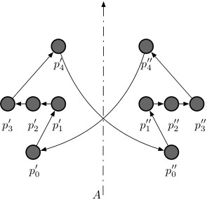
The corresponding ordering pseudocode is defined in Algorithm 4.
The correctness of Algorithm 4 is shown in the following theorem.
Theorem 9.
When and robots do not have chirality, Visit-All is solvable in -step if the initial configuration and one of the following holds:
- 1.
There are no symmetry axes in , or,
- 2.
There exists a unique symmetry axis of and no point of intersects the axis.
Proof.
Algorithm 4 solves the problem. We show its correctness case by case:
- •
There are no symmetry axes in : If , then it is obvious that the robots can agree on a common notion of clockwise direction, and in such a case the order returned at Line 4 is correct by Lemma 1. In case it is possible to agree on a common notion of clockwise direction (Line 3) as follows. Since there exist an ordering among the classes constituting , let be the “highest” class in this order (see red points in Figure 7 as reference). Take a line passing through the centroid of and a point in . Since is not an axis of symmetry, we have that the half-planes defined by are different and not symmetric w.r.t. to . Specifically, it is possible to order them using by scanning the plane starting from in the local clockwise and counter-clockwise directions using as center and stopping at the first asymmetry. Therefore, the half-planes can be used to define a common clockwise direction, e.g., the one going from the lowest half-plane to the highest. Note that this procedure gives the same order for any choice of . Once there is an agreement on clockwise direction the correctness derives from the one of Algorithm 2 (see Lemma 1).
- •
There exists a unique symmetry axis of and no point of intersects : this case starts at Line 5. Let and be partitions of such that is the symmetric of w.r.t. . First of all, we show that robots can agree on a total order on points in : given the axis they can agree on an orientation of the axis (suppose the contrary, then there should exists a second axis intersecting , that is excluded by hypothesis). We order the robots using the coordinates on from lowest to highest (robots with the same coordinate are ordered by their distance from the axis). Let this order be . The analogous can be done for , let this order be . An example is in Figure 9. We merge these two orders by taking the first point in , let it be , the last point in , let it be , and by creating a common cyclic order on which follows . Symmetrically, the first point in follows the last point in .
∎
Interestingly, without chirality, Visit-All is not solvable if the assumptions of Th. 9 do not hold:
Theorem 10.
When and there is no chirality, there exists no algorithm that solves Visit-All in -step from an initial configuration if one of the following holds:
- •
- •
There exists a symmetry axis of intersecting a proper non-empty subset of .
- •
There are at least two symmetry axes of .
Proof.

We prove the impossibility case by case:
- •
: this case derives directly from Theorem 2.
- •
There exists a symmetry axis in and intersects a proper non-empty subset of : to solve Visit-All we must have that a robot outside of axis eventually moves to a position on the axis, let such a position be . However, being a symmetry axis, we must have a robot symmetric to w.r.t. . Robot also moves to position . Since both robots move to point we reach a configuration that is not in .
- •
There are at least two symmetry axes in : let and be these axes. Let be the portions of the plane defined by the axes, see Figure 10. We can assume that no point in intersects the axis (otherwise we are in the previous case). Let be a robot in , and let be the symmetric robots with respect to axis , and both axes (see always Figure 10 for a reference), and let be their respective positions in . Let us suppose, by contradiction, that there exists an algorithm solving Visit-All on , and let be the corresponding run. We examine the path of robot among the points in in the run . Let us suppose, w.l.o.g., that in robot moves to a point in (see the blue dotted path in the Figure 10). It is obvious that the local coordinate systems of the robots could be such that: robot will do a symmetric move to a point in , robot a symmetric move to (see the red path in Figure 10), and so on. Let be the first round at which moves to a location in . Since solves Visit-All such a round must exist, and w.l.o.g let us suppose that visits first the location . By symmetry considerations we have that, at round , also robot has to move to location (recall that is the location occupied by in ). Therefore, from round to robots and have walked on a closed path, let it be , between some locations of that includes and but which does not include (this comes directly from the definition of ). The path is represented in Figure 10 as the union of the red path, the blue paths and the clouds; clouds represent the move made by and between rounds and . Since is an algorithm for oblivious robot, this implies that robots and will only visit points in also in future rounds. Therefore, cannot be correct.
∎
To summarize, we have the following:
Theorem 11.
In systems without chirality, Visit-All is solvable in -step if and only if and either there are no symmetry axes in , or there exists a unique symmetry axis that does not intersect any point of .
4.3 -step Algorithms
In this section we show that using -step algorithms does not help in enlarging the class of solvable configurations.
4.3.1 Move-All
Obviously, Theorem 4 holds also when there is no chirality. One may wonder whether is possible to solve Move-All with a -step algorithm when has a symmetry axis with a unique robot on it. However, the argument used in Theorem 4 can be adapted also for this case showing that this is impossible.
Theorem 12.
When there exists an axis of symmetry in containing a single robot and there is no chirality, then there exists no -steps algorithm that solves Move-All.
Proof.
Consider a configuration and let be an axis with a single robot on it. Let us assume that algorithm is a correct -step algorithm that solves Move-All starting from , and let . Let be the robot in and let be its position. In configuration robot has to move to break the symmetry in such a way that in configuration another robot could substitute on . Suppose the contrary, if remains on the axis in the all the other robots will be symmetric. Therefore, in is not possible for a single robot, different than , to reach position . Therefore let be the position of in .
Let be the robot that exchanges position with in configuration . It is clear that if has a different local coordinate system than , then in configuration it will move to a position . Therefore, we have , violating the Move-All specification (see Lemma 1). ∎
From the previous theorem and Theorem 4, we have:
Theorem 13.
When the system has no chirality, Move-All is not solvable in -steps, from an initial configuration , if , or if there exists an axis of symmetry in containing a single robot.
4.3.2 Visit-All
Theorem 14.
When and there is no chirality, Visit-All is not solvable in -steps, from an initial configuration , if one of the following holds:
- •
- •
There exists a symmetry axis of intersecting a proper non-empty subset of .
- •
There are at least two symmetry axes of .
Proof.
We prove the theorem case by case:
- 1.
: this case derives directly from Theorem 4.
- 2.
There exists a symmetry axis in and it intersects a proper non-empty subset of .
Let us assume that algorithm is a correct -step algorithm that solves Visit-All starting from , and let . It is clear that, to break the symmetry, in each configuration , with odd, the symmetry has to be broken by moving one of the robots located on the symmetry axis. Let be the position of this robot in , note that such a position is the always the same: the decision on which robot has to move is taken always on configurations that are permutations of , thus it will always move a robot to the same specific position. Let and be two robots with different local references systems. Since solves Visit-All there must exist a configuration where robot is in position ; analogously, there must exist a where robot is in position . In configuration robot has to move outside of the axis. The same happens to in configuration . However, the coordinate systems could be such that , and by Lemma 1, this violate the specification of Visit-All: and decides where to move by looking at exactly the same snapshot; therefore, they will move on opposite locations of the axis if their local coordinate systems have opposite chirality. - 3.
There are at least two symmetry axes of : first of all we can assume that it does not exist an axis of containing robots, otherwise we boil down to previous case. For any possible movements of robots, they have to keep the same symmetry. This implies that the argument of Thm. 10 still applies.
∎
5 Oblivious Robots with Visible Coordinate Systems and Chirality
In this section, we assume that each robot can see the coordinate system of all robots and the system has chirality. As we have seen in Section 3, with chirality, the only configurations in which Visit-All cannot be solved are the ones in . We now present a Voting algorithm that solves Visit-All also starting from these configurations, provided that robots have this extra knowledge of the coordinate systems of other robots. The algorithm (see Algorithm 5) uses Procedure innerPolygon, which takes a configuration and returns only the points on the smallest non degenerate circle having the same center as and passing through at least one point of (e.g. see the white points in Figure 11(a)).
When , the algorithm uses the Order procedure from Section 3. In case the initial configuration is in , the algorithm implements a voting procedure to elect a unique vertex of the innermost non-degenerate polygon computed by Procedure innerPolygon. (see, an example in Figure 16). The vote of a robot is computed by translating its coordinate system to the center of . The vote of will be given to the point of that forms the smallest counter-clockwise angle with the -axis of the translated system. Since the number of robots is co-prime to the size of , a unique vertex (robot) can be elected and the elected point is used to break the symmetry and compute a total order among the robots. As before, the robots use this total order to move cyclically solving Visit-All.
Theorem 15.
If each robot can see the axes of the others and there is chirality, then there exists a -step algorithm solving Visit-All for any initial configuration .
Proof.
We have to prove the correctness of Algorithm 5 only for configurations in . Let be the symmetricity of the initial configuration without the central robot, and let be the innermost non degenerate -gon in with .
The key observation is that for some . We now show that no matter which robot calls procedure Voting, the procedure returns always the same point in . Voting iterates over all robots, and computes the vote of each robot . The vote is computed by first translating the coordinate system of to the center of configuration and then taking as voted robot , the one that makes the smallest counter-clockwise angle with the -axis of the translated coordinate system. An example of the voting procedure is in Figure 11. First of all note that the result of the Voting procedure is independent from the robot that is executing it, and it always returns the same distribution of votes for points in , even if we permute the robots in .
We now show that the distribution of votes cannot be symmetric, and one robot in can be elected.
The proof is by contradiction. Let us assume that there exists an axial symmetry on the distribution of votes. The symmetry axis may cross two robots, one robot, or none. In case it crosses only one robot, then we elect that robot as leader. If the axis crosses two robots or none, then the number of votes must be even and so the number of points in , that is ; but this is obviously impossible since and are co-prime.
Let us assume that there exists a rotational symmetry on the votes. Then, there exists a proper divisor of and an ordering of the robots in such that , where is the number of votes for a point of in position of the aforementioned ordering. Notice that this would imply that and are not co-prime, which is a contradiction.
It follows that it is always possible to elect a leader in using the votes.
Therefore, procedure Voting returns the same leader robot for any permutation of the robots in . It is obvious that the presence of breaks the symmetry of the configuration and it allows to compute a total order among positions in shared by all robots. Once this total order is given the solution is immediate. ∎
6 Robots with one bit of Persistent Memory
Motivated by the impossibility result of Theorem 4, we investigate robots with some persistent memory. Interestingly, we show that a single bit of memory is sufficient to overcome the impossibility, and solve Visit-All using a -step algorithm. Note that we cannot overcome the impossibility using -step algorithms, as Theorem 2 holds even if the robots are equipped with an infinite amount of memory.
We present the -step algorithm below (Algorithm 6) for robots.
Intuitive description of the algorithm. The general idea is to use alternate rounds of communication and formation of the actual permutation. In the communication round, the robots create a special intermediate configuration that provides a total order on the robots; In the subsequent round they reconstruct the initial pattern forming the permutation of the initial configuration. The memory bit is crucial to distinguish the intermediate configuration from the initial configuration. If the initial configuration then the robots follow the 1-step algorithm described in Section 3 and we will show that this does not conflict with the rest of the algorithm designed for the case when , as described below.
Initially every robot has the bit set to . When a robot observes that the configuration is in and bit is , it sets the bit to to remember that the initial configuration . The central robot in takes the role of and performs a special move to create the intermediate configuration that is not in but from , it is possible to reconstruct the initial configuration or any permutation of it (This move is determined by procedure ComputeMovementCentral described in the next paragraph).
A key point of the algorithm is that the robot remains invariant. At the next activation, the robots observe a configuration that is not in and they have bit ; this indicates that this is an intermediate configuration and the robots move to reconstruct a configuration . With the exception of the Leader whose memory bit is always set to , all the other robots will now reset their bit to 0.
In the next round, the robots are in configuration , where the central robot is not (the robots have performed one cyclic permutation). At this point, the robot is the unique robot whose bit . All other robots have and they behave similarly as in the first round, including robot which moves like the central robot moved in . However, the leader robot also moves at the same time, in a special way (as described in procedure ComputeMovementNotCentral presented in the next paragraph). The combination of moves of the leader robot and the central robot allows the robots not only to reconstruct the initial configuration, but also to uniquely identify a “pivot” point in the pattern (see Figure 14), which is kept invariant during the algorithm. The reconstruction is executed by procedure Reconstruct whose details are discussed below. The recognition of the pivot point allows the robots agree on the same cyclic ordering of the points in the initial pattern, thus allowing cyclic permutations of the robots.
A pictorial representation of the algorithm is presented in Figure 12.
Movements of and . This paragraph discusses the implementation details of functions ComputeMovementCentral and ComputeMovementNotCentral used in Algorithm 6. In particular, special care has to be taken to design the movements of the robot leader and of the central robot , if different from . Such movements have to be done in such a way to break the symmetry of the configuration by electing always the same pivot position , and to make the central configuration reconstructable. Let be a generic central configuration in . Let be a decomposition of in concentric circles, where each is a circle, is the degenerate circle constituted by the only central robot, and is the innermost non-degenerate polygon on which resides (see Figure 13).
The function ComputeMovementCentral, called by robot , executes the following movements according to the number of robots :
- •
(Case C1): In such a case, since , the robots are on a single line. Let be the segment containing all robots. Robot moves perpendicularly to of a distance . The direction is chosen such that the pivot position will be the one of the first robot encountered travelling along the arcs that connect the endpoints of and in the clockwise direction (see Figure 16(a)).
Figure 14: Movement of the central robot : it moves towards position of a distance that is much smaller than the radius of . The pivot point is on - •
(Case C2): Robot chooses a robot position on as pivot. It moves on the segment connecting and of a small distance (much smaller then the radius of ). See Figure 14.
Robot , when different from , executes the following movements according to (such movements are computed by the function ComputeMovementNotCentral):
- •
. (Case L1): (Robots on a single line): Robot moves on by a small distance, creating a new segment . The pivot position will be indicated by the direction that goes from the old center of to the new center of (see Figure 16(b)).
- •
(case L2): We have three sub-cases depending on which robot is positioned, and on the number of other robots on . Note that (otherwise it would be central). Remember that is the outermost circle, and it coincides with the SEC of . We treat each as a set, e.g. indicates the number of robots/positions in . Let be the difference between the radii of and , and let be the segment connecting and robot . Let be the position of the first robot on encountered by walking in clockwise direction starting from the intersection between and . Let be the number of positions between and the robot that wants to indicate. Recall that is the robot that will move towards if was in .
- –
Sub-case (L2.1). When or and : Robot moves on towards by a quantity . Where is an appropriate function from to . See Figure 15(a) for an example.
- –
Sub-case (L2.2). When and : Note that has to be rotationally symmetric; therefore it contains robots each of them forming an angle of with its adjacent neighbours. Robot moves to a point of that creates with its counter-clockwise neighbour an angle that is , where is an appropriate function from to . See Figure 15(b) for an example.
- –
Sub-case (L2.3). When and : let be the segment connecting the two robots on . Robot moves on , expanding in such a way that the new diameter is , where is an appropriate function from to . See Figure 15(c) for an example.
Note that is not possible to have , since is rotationally symmetric.
- –
It is easy to see that when (or and ) move, the resulting configuration is not in .
Reconstruction of the initial configuration. When the current configuration is not in and the robots have bit , the robots know that they are in an intermediate configuration and they have to (1) reconstruct the original configuration , (2) determine the pivot point in , and (3) identify the leader robot . The reconstruction is performed by procedure Reconstruct, which again, depends on the value of .
- •
In case : the robots are forming a triangle. The base of the triangle is its largest edge . The algorithm uses the height of the triangle, w.r.t. the base to understand if was or not (see Figure 16(c)).
- –
If the height of the triangle is exactly half of , the algorithm infers that and that the two other robots are the endpoints of , case (C1). The pivot is the point of the first clockwise robots encountered following the arc that includes robot and the other two. The original configuration is easily reconstructed: the endpoints of are in the same position, and the central robot will be in the intersection of the perpendicular segment that goes through and .
- –
If the height is slightly less, or slightly more, than the largest edge . Then the algorithm infers that was one of the endpoint; we are in case (L1.1). The reconstruction of is simple: take the intersection of the perpendicular segment that goes through and , the position of the endpoints in is reconstructed using the fact that the hight of the triangle is exactly half of the original segment, and that was the center of the original segment. Robot is the endpoint that moved, and the position is decided evaluating if moved towards or away from the old center.
- –
- •
In case : The algorithm starts by examining , in order to understand if was on the SEC and executed the sub-case (L2.2) or (L2.3). If the test is negative it proceeds using an ‘‘onion peeling” approach, in which the algorithm, starting from the outermost , progressively examines each until it finds an asymmetry or it reaches . The onion peeling proceeds by first computing the SEC, that is , and then computing each by finding progressively smaller concentric circles.
- –
Test for case (L2.3): This test case is done only on . If the center of is not contained in SEC, then the algorithm detects case (L2.3). is adjusted to a new one that has the diameter equal to the distance between the two furthest robots on . Robot will be the robot on that is farthest from robots in . The reconstruction of the last layer is done by knowing that it will be a circle with the same center of SEC that passes through and finally will be indicated by decoding the information encoded in the diameter of .
- –
Test for case (L2.2): This test case is done only on . If and it is not rotationally symmetric, and ( or ), then the algorithm detects case (L2.2). Robot is one that is not forming an angle of radians with any of it adjacent neighbours, position is encoded in the smallest angle that is forming. The original position of can be easily reconstructed: it is the one that forms an angle of with each of its adjacent robots.
- –
Test for case (L2.1): This test case is done on layers different than . If then the algorithm detects case (L2.1). Robot is the only robot in the reconstruction and the detection of are trivial.
If the algorithm reaches not finding an asymmetry then we have that , case (C2). The decoding is trivial: the original position of is the center of , position is the one it moved towards. Note that the algorithm uses always robot to get robot , in case also moves. However, the original position of is always trivial to reconstruct (the center of any with ).
- –
Theorem 16.
There exists an universal algorithm to solve Visit-All for robots with bit of persistent memory.
Proof.
We analyse the correctness of the proposed solution considering three cases:
- •
- •
When the robots start in a configuration and . In this case, for any central configuration reached we may alternate between two different scenario: (S1) only the central robot moves; (S2) two robots move. Scenario (S1) happens in the first configuration, and each time robot goes back to the central position. Scenario (S2) happens each time we are in a central configuration, but is not the central robot. We now prove the correctness for each of the aforementioned possibilities, and this is done by showing that robots start from a configuration , they reach a configuration , and then again a configuration that is a cyclic permutation of .
- –
Scenario (S1), only the central robot moves. At the beginning, the robots have bit and the configuration is , this implies that only the central robot move, see line 12 of Algorithm 6, all the robots set their bit . The central robot moves of a small distance towards a robot . At the next round, the robots will se a , but since they know that they started from a central configuration, see line 18. Notice that, if moved of a small distance still being inside the circle formed by the innermost robots (see as reference Figure 12) then it is simple for all robots to reconstruct the proper by seeing and executing the Reconstruct procedure. Therefore, they can understand that is the only robot that moved and everyone appoints as leader, it also simple to identify the pivot robot in the innermost circle of .
- –
Scenario (S2), only two robots move. Robots that change position are the central robot (line 12 of Figure 6), and the only one that started the round with bit that is robot (line 15 of Figure 6). Before ending the round, all the robots set their bit (line 11). The movement of robot is different depending on its position. The purpose of this move is to indicate the pivot robot , that would have chosen if it was the central robot. After and moved, we are in a configuration and all robot have bit set, so they can remember they were starting from a central configuration. The only item left to show is that they can all reconstruct the central configuration and they can all agree on robot being the leader. We now show that the robots do reconstruct starting from and thus agree on the same cyclic order. The reconstruction is done by the procedure Reconstruct. We have to show that for each possible case the reconstruction is correct.
- *
Reconstruction from a configuration created with move (L2.1). First of all the algorithm cannot mistake it for cases (L2.2) and (L2.3). The correct reconstruction is immediate.
- *
Reconstruction from a configuration created with move (L2.2). The case cannot be mistaken for (L2.3): the SEC is concentric with the other . It cannot be mistaken for case L2.1: or . The reconstruction is immediate.
- *
Reconstruction from a configuration created with move (L2.3). This case is detected by observing that the centre of SEC is not contained in SEC. This happens only when moved according to rule (L2.3). The Reconstruct adjusts the SEC, that contains three robots, to a new sec that has as diameter the two furthest robots on the old SEC. Let and be the two robots on the new . We argue that the distance of this two robots is encoding the position . Refer to Figure 15(c): robot moves from the other robots up to a distance . By doing so, it is becoming the robot that is furthest from all the others in . It is also clear that the by removing and we get (neglecting for now the central robot). The diameter can be recovered by taking the circle with center in SEC and passing through . With this information the decoding is simple, and the reconstruction of is immediate.
- *
- –
When the robots start in a configuration and : In this case when the configuration is in the movements of the central robot and of the leader robot follow special rules. Notice that all three robots lie on a segment . Robot moves following case (L2.1) if is not central. The central robot moves according to case (C2). It easy to see that the robots reconstruct the central configuration and they correctly elect the leader, which is either the central robot (if it is the only robot that moved) or the external robot (if two robots moved). It is also immediate that Visit-All is solved, since robots execute continuously the same cyclic permutation.
Once are known the robots agree on the same cyclic order and reach a new configuration . An immediate induction shows that starting from the initial configuration we alternate either in scenario S1 or S2 solving Visit-All.
- –
∎
7 Concluding Remarks
To the best of our knowledge, this is the first investigation of the problems of permuting the positions of a set of mobile robots in the plane. Surprisingly this class of problems seems to be more difficult than the previously studied problems such as gathering and pattern formation, which have easy solutions for the strongest model of fully synchronous robots with rigid movements. Thus the characterization of solvable instances for permutation problems is quite different as shown in this paper. Moreover we also showed that being non-oblivious is helpful for permuting robots, unlike the formation problems where the solvability is unaffected by obliviousness [20].
The paper opens several research directions that are worth investigating: an interesting direction would be to discover other class of problems which cannot be solved even when it is easy to elect a leader (as the class of problems considered here). The difficulty in solving the permutation problems seems to be unrelated to agreement problems such as leader election. In particular we may try to study the differences between leader election and permutation problems and determine if the latter is strictly more difficult than the former. We may also consider other interesting assumptions that can help in overcoming the challenges for permuting robots without orientation. One possibility is the investigation of robots with the additional capability of communicating using visible lights [5, 7, 10].
Acknowledgements: This work has been partially funded by the University of Rome “La Sapienza” with the Calypso project. Some of the authors were supported in part by NSERC Canada through the Discovery Grants program and by Prof. Flocchini’s University Research Chair.
References
- [1] H. Ando, I. Suzuki, and M. Yamashita. Formation and agreement problems for synchronous mobile robots with limited visibility. In Proc. of the 10th IEEE Symp. on Intelligent Control, pages 453–460, 1995.
- [2] Q. Bramas and S. Tixeuil. Brief announcement: Probabilistic asynchronous arbitrary pattern formation. In Proc. of the 34th ACM Symposium on Principles of Distributed Computing (PODC), pages 443–445, 2016.
- [3] S. Cicerone, G. Di Stefano, and A. Navarra. Asynchronous embedded pattern formation without orientation. In Proc. of the 30th International Symposium on Distributed Computing (DISC), pages 85–98, 2016.
- [4] S. Cicerone, G. Di Stefano, and A. Navarra. Gathering of robots on meeting-points: feasibility and optimal resolution algorithms. Distributed Computing 31(1): 1–50, 2018.
- [5] S. Das, P. Flocchini, G. Prencipe, N. Santoro, and M. Yamashita. Autonomous mobile robots with lights. Theoretical Computer Science, 609(P1):171–184, January 2016.
- [6] S. Das, P. Flocchini, N. Santoro, and M. Yamashita. Forming sequences of geometric patterns with oblivious mobile robots. Distributed Computing, 28(2):131–145, April 2015.
- [7] G.A. Di Luna, P. Flocchini, S. Gan Chaudhuri, F. Poloni, N. Santoro, G. Viglietta, Mutual visibility by luminous robots without collisions, In Information and Computation 254(3) 392–418, 2017.
- [8] G. Di Luna, P. Flocchini, N. Santoro, G. Viglietta. TuringMobile: A turing machine of oblivious mobile robots with limited visibility and its applications. In Proc. of the 32nd International Symposium on Distributed Computing (DISC), pages 19:1-19:15, 2018.
- [9] G. Di Luna, P. Flocchini, N. Santoro, G. Viglietta, and M. Yamashita. Meeting in a polygon by anonymous oblivious robots. In Proc. of the 31st International Symposium on Distributed Computing (DISC), pages 14:1-14:15, 2017.
- [10] G. Di Luna, G. Viglietta. Robots with lights. In Distributed Computing by Mobile Entities: Current Research in Moving and Computing, pages 252-277, 2019.
- [11] M. Erdelj, T. Razafindralambo, and D. Simplot-Ryl. Covering points of interest with mobile sensors. IEEE Transactions on Parallel and Distributed Systems 24(1):32–43, 2013.
- [12] P. Flocchini, G. Prencipe, and N. Santoro. Distributed Computing by Oblivious Mobile Robots. Morgan & Claypool, 2012.
- [13] P. Flocchini, G. Prencipe, N. Santoro, and P. Widmayer. Arbitrary pattern formation by asynchronous oblivious robots. Theoretical Computer Science, 407(1-3):412–447, 2008.
- [14] P. Flocchini, N. Santoro, G. Viglietta, and M. Yamashita. Rendezvous with constant memory. Theoretical Computer Science, 621:57–72, 2016.
- [15] N. Fujinaga, Y. Yamauchi, H. Ono, S. Kijima, and M. Yamashita. Pattern formation by oblivious asynchronous mobile robots. SIAM Journal on Computing, 44(3):740–785, 2015.
- [16] N. Fujinaga, Y. Yamauchi, S. Kijima, and M. Yamashita. Asynchronous pattern formation by anonymous oblivious mobile robots. In Proc. of the 26th International Symposium on Distributed Computing (DISC), pages 312–325, 2012.
- [17] G. Sharma, C. Busch, and S. Mukhopadhyay. Mutual visibility with an optimal number of colors. In 11th International Symposium on Algorithms and Experiments for Wireless Sensor Networks (Algosensors), pages 196–201, 2015.
- [18] K. Sugihara and I. Suzuki. Distributed algorithms for formation of geometric patterns with many mobile robots. Journal of Robotics Systems, 13:127–139, 1996.
- [19] I. Suzuki and M. Yamashita. Distributed anonymous mobile robots: Formation of geometric patterns. SIAM Journal on Computing, 28(4):1347–1363, 1999.
- [20] M. Yamashita and I. Suzuki. Characterizing geometric patterns formable by oblivious anonymous mobile robots. Theoretical Computer Science, 411(26-28):2433–2453, 2010.
- [21] Y. Yamauchi and M. Yamashita. Randomized pattern formation algorithm for asynchronous oblivious mobile robots. In Proc. of the 28th International Symposium on Distributed Computing (DISC), pages 137–151, 2014.