Experience-Embedded Visual Foresight
Abstract
Visual foresight gives an agent a window into the future, which it can use to anticipate events before they happen and plan strategic behavior. Although impressive results have been achieved on video prediction in constrained settings, these models fail to generalize when confronted with unfamiliar real-world objects. In this paper, we tackle the generalization problem via fast adaptation, where we train a prediction model to quickly adapt to the observed visual dynamics of a novel object. Our method, Experience-embedded Visual Foresight (EVF), jointly learns a fast adaptation module, which encodes observed trajectories of the new object into a vector embedding, and a visual prediction model, which conditions on this embedding to generate physically plausible predictions. For evaluation, we compare our method against baselines on video prediction and benchmark its utility on two real world control tasks. We show that our method is able to quickly adapt to new visual dynamics and achieves lower error than the baselines when manipulating novel objects.
Keywords: Video Prediction, Model-based Reinforcement Learning, Deep Learning
1 Introduction
The ability to visualize possible futures allows an agent to consider the consequences of its actions before making costly decisions. When visual prediction is coupled with a planner, the resulting framework, visual model-predictive control (visual MPC), can perform a multitude of tasks – such as object relocation and the folding of clothes – all with the same unified model [1, 2].
Like any learned model, visual MPC works very well when predicting the dynamics of an object it has encountered many times in the past, e.g., during training. But when shown a new object, its predictions are often physically implausible and fail to be useful for planning.
This failure contrasts with the ability of humans to quickly adapt to new scenarios. When we encounter a novel object, we may initially have little idea how it will behave – is it soft or hard, heavy or light? However, just by playing with it a bit, we can quickly estimate its basic physical properties and begin to make accurate predictions about how it will react under our control.
Our goal in this paper is to develop an algorithm that learns to quickly adapt in a similar way. We consider the problem of few-shot visual dynamics adaptation, where a visual prediction model aims to better predict the future given a few videos of previous interactions with an object.
To that end, we propose Experience-embedded Visual Foresight (EVF), where adaptation is performed via an experience encoder that takes as input a set of previous experiences with the object, in the format of videos, and outputs a low-dimensional vector embedding, which we term a “context”. This embedding is then used as side information for a recurrent frame prediction module. Our method is centered on the idea that there is an embedding space of objects’ properties, where similar objects (in terms of visual dynamics) are close together while different objects are far apart. Having such a space allows for few-shot visual dynamics adaptation and opens the possibility of inferring information from new and unfamiliar objects in a zero-shot fashion.
Our approach can further be formalized as a hierarchical Bayes model in which object properties are latent variables that can be inferred from a few prior experiences with the object. The full system, as shown in Figure 1, is trained end-to-end and therefore can be understood as a form of meta-learning: under this view, the experience encoder is a fast learner, embodied in a feedforward network that modulates predictions based on just a few example videos. The weights of this fast learner are themselves also learned, but by the slower process of stochastic gradient descent over many meta-batches of examples and predictions.
EVF can be categorized as “learning from observations” [3, 4], rather than “learning from demonstrations, as it does not require that observed trajectories contain actions. This means it can utilize experiences when actions are unknown or generated by an agent with a different action-space.
To evaluate our approach, we compare EVF against baselines which apply gradient-based meta-learning [5] to video prediction, and validate that our method improves visual MPC’s performance on two real-world control tasks in which a robot manipulates novel objects.
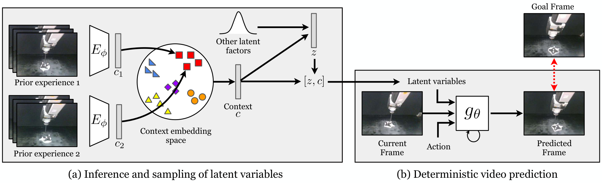
Our contributions include:
- 1.
A hierarchical Bayes model for few-shot visual dynamics adaptation.
- 2.
Improved performance on both video prediction and model-based control.
- 3.
A learned video representation that captures properties related to object dynamics.
2 Related Work
Embedding-based Meta Learning.
Learning an embedding function to summarize information from a few samples has shown promising results for few-shot learning tasks. For image classification, Matching Networks [6] learns an embedding space to compare a few labeled examples with testing data, and builds a classifier based on weighted nearest neighbor. Similarly, Prototypical Networks learns an embedding space but instead represents each class by the mean of its examples (a prototype). Then, a classifier is built using squared Euclidean distances between testing data’s embedding and different classes’ prototypes. For visuomotor control, TecNets [7] learns an embedding space of demo trajectories. During test time, it feeds the trajectory embeddings into a control network to perform one-shot imitation learning. We adopt a similar approach but apply it to visual MPC rather than to imitation learning. For generative modelling, Neural Statistician [8] extends the variational autoencoder (VAE) [9] to model datasets instead of individual datapoints, where the learned embedding for each dataset is used for the decoder to reconstruct samples from that dataset. Our method extends Neural Statistician [8] to model visual dynamics of diverse objects. The learned model is also used for model-based control.
Model-based Reinforcement Learning.
Algorithms which learn a dynamics model to predict the future and use it to improve decision making belong to the category of model-based reinforcement learning (RL). Lately, visual model-based RL has been applied to real world robotic manipulation problems [1, 2, 10, 11]. However, these methods do not focus on adaptation of the visual prediction model. A few recent works have explored combining meta-learning with model-based RL in order to adapt to different environments in low-dimensional state space [12, 13]. In this work, we tackle the problem of adapting high-dimensional visual dynamics by learning a latent space for object properties, inspired by previous works on metric-based meta learning [6, 7].
Video Prediction.
The breakthrough of deep generative models [14, 9, 15] has lead to impressive results on deterministic video prediction [16, 17, 18, 19, 20]. Specifically, action-conditioned video prediction has been shown to be useful in video games [21, 22] and robotic manipulation [1, 2, 23, 24]. Our work is most similar to approaches which perform deterministic next frame generation based on stochastic latent variables [25, 26, 27, 28]. The main difference between these works and ours is shown in Figure 2. Rather than learning a generative model for all the videos in a single dataset, we construct a hierarchical Bayes model to learn from many small yet related datasets [8, 29]. Our goal is to robustify visual MPC’s performance by adapting to unseen objects.
3 Preliminaries
In visual MPC (or visual foresight), the robot first collects a dataset which contains trajectories. Each trajectory can further be represented as a sequence of images and actions . Then, the dataset is used to learn an action-conditioned video prediction model that approximates the stochastic visual dynamics . Once the model is learned, it can be coupled with a planner to find actions that minimize an objective specified by user. In this work, we adopt the cross entropy method (CEM) as our planner and assume the objective is specified as a goal image. At the planning stage, CEM aims to find a sequence of actions that minimizes the difference between the predicted future frames and the goal image. Then, the robot executes the first action in the planned action sequence and performs replanning.
4 Method
Our goal is to robustify visual MPC’s performance when manipulating unseen objects through rapid adaptation of visual dynamics. Inspired by previous works, we hypothesize that humans’ capability of rapid adaptation is powered by their ability to infer latent properties that can facilitate prediction. To endow our agent the same capability, we consider a setting different from prior work where we are given datasets for . Each dataset contains trajectories of the robot interacting with a specific environment. We assume there is a common underlying generative process such that the stochastic visual dynamics for dataset can be written as for drawn from some distribution , where is a “context” embedding. Intuitively, the context shared by all trajectories in a dataset captures environmental information that generates the dataset, e.g., an object’s mass and shape.
Our task can thus be split into generation and inference components. The generation component consists of learning a model that approximates the underlying generative process . To model stochasticity, we introduce latent variables at each time step to carry stochastic information about the next frame in a video. The inference component learns an approximate posterior over the context . Since encoding the whole dataset is computationally prohibitive, we construct a support set which contains trajectories sub-sampled from and learn a function to estimate from . In our experiments, is a small number, . We denote a trajectory, image, and action in the support set as , and . The rightmost subfigure of Figure 2 shows the graphical model of our method. Overall, our learning approach is an extension of VAE, and we detail this formalism in Section 4.2.

4.1 Overview
Before detailing the training procedure, we explain how our method performs adaptation and generates predictions for unseen objects. To adapt the video prediction model, we first use the inference component, i.e., an experience encoder with parameters , to encode videos in the support set into an approximate posterior over context. Then, we sample a context from this posterior and feed it into our generation component to produce predictions. Our generation component is an action-conditioned video prediction model parameterized by , that generates the next frame , based on previous frames , action , stochastic latent variables , and context .
The two components are trained end-to-end jointly with the aid of a separate frame encoder (not used at test time). To train our model, we again first sample from the approximate posterior constructed by the experience encoder. Then, the frame encoder encodes , i.e., the target of the prediction model, along with previous frames and to compute another distribution from which we sample . By assuming the prior of the context and the latent variable to be normally distributed, we force and to be close to the corresponding prior distribution and using KL-divergence terms. These two terms constrain the information that and can carry, forcing them to capture useful information for prediction. In addition, we have another term in our loss to penalize the reconstruction error between and .
4.2 Variational Auto-encoders Over Sets
To further explain our model, we adopt the formalism of variational auto-encoders over sets [8, 29]. For each trajecory , the likelihood given a context can be written as:
| (1) |
However, this likelihood cannot be directly optimized as it involves marginalizing over the latent variables , which is generally intractable. Therefore, the frame encoder is used to approximate the posterior with a conditional Gaussian distribution . Then, the likelihood of each trajectory in a dataset can be approximated by the variational lower bound:
| (2) |
Note that although Eq. (2) can be used to maximize the likelihood of trajectories in a single dataset [25, 26, 27], our goal is to approximate the commonly shared generative process through maximizing the likelihood of many datasets. Based on the graphical model plotted on the right in Figure 2, the likelihood of a single dataset can be written as:
| (3) |
In order to solve the intractability of marginalizing over the context , we introduce an experience encoder which takes as input the whole dataset to construct an approximate posterior over context. By applying variational inference, we can lower bound the likelihood of a dataset with:
| (4) |
The hyper-parameters and represent the trade-off between minimizing frame prediction error and fitting the prior. Taking smaller and increases the representative power of the frame encoder and the experience encoder. Nonetheless, both may learn to simply copy the target frame if or are too small, resulting in low training error but struggling to generalize at test time.
4.3 Stochastic Lower Bound
Note that in Eq. (4), calculating the variational lower bound for each dataset requires passing the whole dataset through both inference and generation components for each gradient update. This can become computationally prohibitive when a dataset contains hundreds of samples. In practice, since we only pass a support set subsampled from , the loss is re-scaled as follows:
| (5) |
In this work, we sample 5 trajectories without replacement to construct the support set .
4.4 Model Architectures
We use SAVP [27] as our backbone architecture for the generation component. Our model is a convolutional LSTM which predicts the transformations of pixels between the current and next frame. Skip connections with the first frame are added as done in SNA [23]. Note that at every time step , the generation component only receives , , , and as input. The dependencies on all previous and stem from the recurrent nature of the model. To implement the conditioning on action, latent variables, and context, we concatenate them along the channel dimension to the inputs of all the convolutional layers of the LSTM. The experience encoder is a feed-forward convolutional network which encodes the image at every time step and an LSTM which takes as input the encoded images sequentially. We apply the experience encoder to trajectories in the support set to collect LSTM final states. Sample mean is used as a pooling operation to collapse these states into the mean of our approximate posterior . The frame encoder is a feed-forward convolutional network which encodes and at every time step. We train the model using the re-parameterization trick and estimate the expectation over with a single sample.
5 Experiments
In this section, we aim to answer the following questions: (i) Can we learn a context embedding that facilitates visual dynamics adaptation? (ii) Does the context embedding improve the performance of downstream visual MPC tasks? (iii) Can the context embedding be used to infer similarity between objects?
First we present video prediction results on Omnipush and KTH Action to answer questions (i) and (iii) from section 5.1 to 5.2. Then, we report results on two real world control tasks to answer question (ii) in section 5.3. In our experiments, we compare our method to the following baselines:
- •
- •
SAVP-F. SAVP finetuned with 5 videos in the support set with learning rate 5e-4 for 50 steps.
- •
SAVP-MAML. SAVP trained with MAML [5] and finetuned the same way as in SAVP-F.
We also tried implementing an RNN-based meta-learner [30], where SAVP’s hidden states are not reset after encoding videos from the support set. However, we were not able to achieve improved performance using this method.
5.1 Omnipush Dataset
Our first experiment use Omnipush dataset [31] which contains RGBD videos of an ABB IRB 120 industrial arm pushing 250 objects, each pushed 250 times. For each push, the robot selects a random direction and makes a 5cm straight push for 1s. Using modular meta-learning [32] on ground truth pose data (rather than raw RGBD), the authors showed that Omnipush is suitable for evaluating adaptation because it provides systematic variability, making it easy to study, e.g., the effects of mass distribution vs. shape on the dynamics of pushing.
We use the first split of the dataset (i.e., 70 objects without extra weight) to conduct the experiments. We condition on the first 2 frames and train to predict the next 10. To benchmark the adaptability of our approach, we train on 50 objects and test on the remaining 20 novel objects. Figure 3 shows qualitative results of video prediction. Following previous works [26, 27], we provide quantitative comparisons by computing the learned perceptual image patch similarity (LPIPS) [33], the structural similarity (SSIM) [34], and the peak signal-to-noise ratio (PSNR) between ground truth and generated video sequences. Quantitative results are shown in Figure 4. Our method predicts more physically plausible videos compared to baselines, and especially captures the shape of the pushed object better. We further show that this improves the performance of visual MPC in section 5.3.

Visualization of context embedding.
In Figure 7, we use t-SNE [35] to visualize the context embedding of the 20 novel objects we tested. Despite never seeing these object during training, our model is able to produce a discriminative embedding where objects with similar properties, such as mass and shape, are close together, and those with different properties are far apart.

5.2 KTH Action Dataset
The KTH Action dataset [36] consists of real-world videos of people performing different actions, where each person performs the same action in 4 different settings. We split the dataset into many small datasets according to person and action. Therefore, the support set consists of the other 3 videos belonging to the same small dataset. Following the setting of previous work [27], our models are trained to predict 10 future frames conditioned on 10 initial frames. During test time, it is tested to predict 30 frames into the future. We show qualitative results in Figure 5 and quantitative results in Figure 6.
5.3 Real World Pushing
We perform two types of real-world robotic experiments to verify that predictions generated by our method are more physically plausible, and that this benefits visual MPC. In the first experiment, we ask the robot to perform re-location, where the robot should push an object to a designated pose. In the second experiment, the robot has to imitate the pushing trajectory presented in a 10-second video. In both tasks we use pixel-wise loss, with the robot arm masked, to measure the distance between the predicted image and the goal image. At each iteration of planning, our CEM planner samples 200 candidates and refits to the best 10 samples. The results of this experiment can be found in Table 1. Note that several more advanced loss functions have been recently proposed for visual MPC [24, 23, 2], but we opted for simple to isolate the contribution of our method in terms of improved visual predictions, rather than improved planning.
| Re-positioning | |||
|---|---|---|---|
| Method | Type | Seen | Unseen |
| No motion | mean | 90.4 | 91.9 |
| median | 87.4 | 90.4 | |
| SAVP | mean | 26.2 | 48.4 |
| median | 27.1 | 48.5 | |
| EVF (ours) | mean | 21.8 | 36.2 |
| median | 20.1 | 29.1 | |
| Trajectory-tracking | |||||
|---|---|---|---|---|---|
| Method | Type | Traj 1 | Traj 2 | Traj 3 | Traj 4 |
| No motion | mean | 112 | 93.6 | 91.1 | 97.7 |
| final | 154 | 127 | 137 | 141 | |
| SAVP | mean | 33.5 | 42.7 | 29.5 | 41.2 |
| final | 79.8 | 60.8 | 49 | 59.5 | |
| EVF (ours) | mean | 31.6 | 25.2 | 21.6 | 27.5 |
| final | 59.9 | 47.7 | 48.7 | 48.6 | |
6 Conclusion
In this work, we considered the problem of visual dynamics adaptation in order to robustify visual MPC’s performance when manipulating novel objects. We proposed a hierarchical Bayes model and showed improved results on both video prediction and model-based control. In the future, it would be interesting to investigate how to acticely collect useful data for few-shot adaptation.

Acknowledgments
We thank Alberto Rodriguez, Shuran Song, and Wei-Chiu Ma for helpful discussions. This research was supported in part by the MIT Quest for Intelligence and by iFlytek.
References
- Finn and Levine [2017] C. Finn and S. Levine. Deep visual foresight for planning robot motion. In 2017 IEEE International Conference on Robotics and Automation (ICRA), pages 2786–2793. IEEE, 2017.
- Ebert et al. [2018] F. Ebert, C. Finn, S. Dasari, A. Xie, A. Lee, and S. Levine. Visual foresight: Model-based deep reinforcement learning for vision-based robotic control. arXiv preprint arXiv:1812.00568, 2018.
- Kroemer et al. [2019] O. Kroemer, S. Niekum, and G. Konidaris. A review of robot learning for manipulation: Challenges, representations, and algorithms. CoRR, abs/1907.03146, 2019. URL http://arxiv.org/abs/1907.03146.
- Pathak et al. [2018] D. Pathak, P. Mahmoudieh, G. Luo, P. Agrawal, D. Chen, Y. Shentu, E. Shelhamer, J. Malik, A. A. Efros, and T. Darrell. Zero-shot visual imitation. In Proceedings of the IEEE Conference on Computer Vision and Pattern Recognition Workshops, pages 2050–2053, 2018.
- Finn et al. [2017] C. Finn, P. Abbeel, and S. Levine. Model-agnostic meta-learning for fast adaptation of deep networks. In Proceedings of the 34th International Conference on Machine Learning-Volume 70, pages 1126–1135. JMLR. org, 2017.
- Vinyals et al. [2016] O. Vinyals, C. Blundell, T. Lillicrap, D. Wierstra, et al. Matching networks for one shot learning. In Advances in neural information processing systems, pages 3630–3638, 2016.
- James et al. [2018] S. James, M. Bloesch, and A. J. Davison. Task-embedded control networks for few-shot imitation learning. arXiv preprint arXiv:1810.03237, 2018.
- Edwards and Storkey [2016] H. Edwards and A. Storkey. Towards a neural statistician. arXiv preprint arXiv:1606.02185, 2016.
- Kingma and Welling [2013] D. P. Kingma and M. Welling. Auto-encoding variational bayes. arXiv preprint arXiv:1312.6114, 2013.
- Byravan and Fox [2017] A. Byravan and D. Fox. Se3-nets: Learning rigid body motion using deep neural networks. In 2017 IEEE International Conference on Robotics and Automation (ICRA), pages 173–180. IEEE, 2017.
- Zhang et al. [2018] M. Zhang, S. Vikram, L. Smith, P. Abbeel, M. Johnson, and S. Levine. Solar: deep structured representations for model-based reinforcement learning. 2018.
- Nagabandi et al. [2018a] A. Nagabandi, I. Clavera, S. Liu, R. S. Fearing, P. Abbeel, S. Levine, and C. Finn. Learning to adapt in dynamic, real-world environments through meta-reinforcement learning. arXiv preprint arXiv:1803.11347, 2018a.
- Nagabandi et al. [2018b] A. Nagabandi, C. Finn, and S. Levine. Deep online learning via meta-learning: Continual adaptation for model-based rl. arXiv preprint arXiv:1812.07671, 2018b.
- Goodfellow et al. [2014] I. Goodfellow, J. Pouget-Abadie, M. Mirza, B. Xu, D. Warde-Farley, S. Ozair, A. Courville, and Y. Bengio. Generative adversarial nets. In Advances in neural information processing systems, pages 2672–2680, 2014.
- Oord et al. [2016] A. v. d. Oord, N. Kalchbrenner, and K. Kavukcuoglu. Pixel recurrent neural networks. arXiv preprint arXiv:1601.06759, 2016.
- Mathieu et al. [2015] M. Mathieu, C. Couprie, and Y. LeCun. Deep multi-scale video prediction beyond mean square error. arXiv preprint arXiv:1511.05440, 2015.
- Villegas et al. [2017] R. Villegas, J. Yang, Y. Zou, S. Sohn, X. Lin, and H. Lee. Learning to generate long-term future via hierarchical prediction. In Proceedings of the 34th International Conference on Machine Learning-Volume 70, pages 3560–3569. JMLR. org, 2017.
- Wichers et al. [2018] N. Wichers, R. Villegas, D. Erhan, and H. Lee. Hierarchical long-term video prediction without supervision. arXiv preprint arXiv:1806.04768, 2018.
- Kalchbrenner et al. [2017] N. Kalchbrenner, A. van den Oord, K. Simonyan, I. Danihelka, O. Vinyals, A. Graves, and K. Kavukcuoglu. Video pixel networks. In Proceedings of the 34th International Conference on Machine Learning-Volume 70, pages 1771–1779. JMLR. org, 2017.
- Finn et al. [2016] C. Finn, I. Goodfellow, and S. Levine. Unsupervised learning for physical interaction through video prediction. In Advances in neural information processing systems, pages 64–72, 2016.
- Oh et al. [2015] J. Oh, X. Guo, H. Lee, R. L. Lewis, and S. Singh. Action-conditional video prediction using deep networks in atari games. In Advances in neural information processing systems, pages 2863–2871, 2015.
- Ha and Schmidhuber [2018] D. Ha and J. Schmidhuber. World models. arXiv preprint arXiv:1803.10122, 2018.
- Ebert et al. [2017] F. Ebert, C. Finn, A. X. Lee, and S. Levine. Self-supervised visual planning with temporal skip connections. arXiv preprint arXiv:1710.05268, 2017.
- Xie et al. [2018] A. Xie, A. Singh, S. Levine, and C. Finn. Few-shot goal inference for visuomotor learning and planning. In Conference on Robot Learning, pages 40–52, 2018.
- Babaeizadeh et al. [2017] M. Babaeizadeh, C. Finn, D. Erhan, R. H. Campbell, and S. Levine. Stochastic variational video prediction. arXiv preprint arXiv:1710.11252, 2017.
- Denton and Fergus [2018] E. Denton and R. Fergus. Stochastic video generation with a learned prior. arXiv preprint arXiv:1802.07687, 2018.
- Lee et al. [2018] A. X. Lee, R. Zhang, F. Ebert, P. Abbeel, C. Finn, and S. Levine. Stochastic adversarial video prediction. arXiv preprint arXiv:1804.01523, 2018.
- Kumar et al. [2019] M. Kumar, M. Babaeizadeh, D. Erhan, C. Finn, S. Levine, L. Dinh, and D. Kingma. Videoflow: A flow-based generative model for video. arXiv preprint arXiv:1903.01434, 2019.
- Hewitt et al. [2018] L. B. Hewitt, M. I. Nye, A. Gane, T. Jaakkola, and J. B. Tenenbaum. The variational homoencoder: Learning to learn high capacity generative models from few examples. arXiv preprint arXiv:1807.08919, 2018.
- Duan et al. [2016] Y. Duan, J. Schulman, X. Chen, P. L. Bartlett, I. Sutskever, and P. Abbeel. Rl2: Fast reinforcement learning via slow reinforcement learning. arXiv preprint arXiv:1611.02779, 2016.
- Bauza et al. [2019] M. Bauza, F. Alet, Y. Lin, T. Lozano-Perez, L. Kaelbling, P. Isola, and A. Rodriguez. Omnipush: accurate, diverse, real-world dataset of pushing dynamics with rgb-d video. In IEEE/RSJ International Conference on Intelligent Robots and Systems, 2019.
- Alet et al. [2018] F. Alet, T. Lozano-Pérez, and L. P. Kaelbling. Modular meta-learning. arXiv preprint arXiv:1806.10166, 2018.
- Zhang et al. [2018] R. Zhang, P. Isola, A. A. Efros, E. Shechtman, and O. Wang. The unreasonable effectiveness of deep features as a perceptual metric. In Proceedings of the IEEE Conference on Computer Vision and Pattern Recognition, pages 586–595, 2018.
- Wang et al. [2004] Z. Wang, A. C. Bovik, H. R. Sheikh, E. P. Simoncelli, et al. Image quality assessment: from error visibility to structural similarity. IEEE transactions on image processing, 13(4):600–612, 2004.
- Maaten and Hinton [2008] L. v. d. Maaten and G. Hinton. Visualizing data using t-sne. Journal of machine learning research, 9(Nov):2579–2605, 2008.
- Schüldt et al. [2004] C. Schüldt, I. Laptev, and B. Caputo. Recognizing human actions: a local SVM approach. In Proc. Int. Conf. Pattern Recognition (ICPR’04), Cambridge, U.K, 2004.