Machine Intelligence at the Edge
with Learning Centric Power Allocation
Abstract
While machine-type communication (MTC) devices generate considerable amounts of data, they often cannot process the data due to limited energy and computational power. To empower MTC with intelligence, edge machine learning has been proposed. However, power allocation in this paradigm requires maximizing the learning performance instead of the communication throughput, for which the celebrated water-filling and max-min fairness algorithms become inefficient. To this end, this paper proposes learning centric power allocation (LCPA), which provides a new perspective on radio resource allocation in learning driven scenarios. By employing 1) an empirical classification error model that is supported by learning theory and 2) an uncertainty sampling method that accounts for different distributions at users, LCPA is formulated as a nonconvex nonsmooth optimization problem, and is solved using a majorization minimization (MM) framework. To get deeper insights into LCPA, asymptotic analysis shows that the transmit powers are inversely proportional to the channel gains, and scale exponentially with the learning parameters. This is in contrast to traditional power allocations where quality of wireless channels is the only consideration. Last but not least, a large-scale optimization algorithm termed mirror-prox LCPA is further proposed to enable LCPA in large-scale settings. Extensive numerical results demonstrate that the proposed LCPA algorithms outperform traditional power allocation algorithms, and the large-scale optimization algorithm reduces the computation time by orders of magnitude compared with MM-based LCPA but still achieves competing learning performance.
Index Terms:
Empirical classification error model, edge machine learning, learning centric communication, multiple-input multiple-output, resource allocation.I Introduction
MACHINE intelligence is revolutionizing every branch of science and technology [1, 2]. If a machine wants to learn, it requires at least two ingredients: information and computation, which are usually separated from each other in machine-type communication (MTC) systems [3]. Nonetheless, sending vast volumes of data from MTC devices to the cloud not only leads to a heavy communication burden but also increases the transmission latency. To address this challenge brought by MTC, a promising solution is the edge machine learning technique [4, 5, 6, 7, 8, 9, 10, 11] that trains a machine learning model or fine-tunes a pre-trained model at the edge, i.e., at a nearby radio access point with computation resources.
In general, there are two ways to implement edge machine learning: data sharing and model sharing. Data sharing uses the edge to collect data generated from MTC devices for machine learning [4, 5, 6, 7], while model sharing uses federated learning [8, 9, 10, 11] to exchange model parameters (instead of data) between the edge and users. Both approaches are recognized as key paradigms in the sixth generation (6G) wireless communications [12, 13, 14]. However, since the MTC devices often cannot process the data due to limited computational power, this paper focuses on data sharing.
I-A Motivation and Related Work
In contrast to conventional communication systems, edge machine learning systems aim to maximize the learning performance instead of the communication throughput. Therefore, edge resource allocation becomes very different from traditional resource allocation schemes that merely consider the wireless channel state information [15, 16, 17, 18]. For instance, the celebrated water-filling scheme allocates more resources to better channels for throughput maximization [15], and the max-min fairness scheme allocates more resources to cell-edge users to maintain certain quality of service [16]. While these two schemes have proven to be very efficient in traditional wireless communication systems, they could lead to poor learning performance in edge learning systems because they do not account for the machine learning factors such as model and dataset complexities. Imagine training a deep neural network (DNN) and a support vector machine (SVM) at the edge. Due to much larger number of parameters in DNN, the edge should allocate more resources to MTC devices that upload data for the DNN than those for the SVM.
Nonetheless, in order to maximize the learning performance, we need a mathematical expression of the learning performance with respect to the number of samples, which does not exist to the best of the authors’ knowledge. While the sample complexity of a learning task can be related to the Vapnik-Chervonenkis (VC) dimension [1], this theory only provides a vague estimate that is independent of the specific learning algorithm or data distribution. To better understand the learning performance, it has been proved in [19, 20] that the generalization error can be upper bounded by the summation of the bias between the model’s prediction and the optimal prediction, the variance due to training datasets, and the noise of the target example. With the bound being tight for certain loss functions (e.g., squared loss and zero-one loss), the bias-variance decomposition theory gives rise to an empirical nonlinear classification error model [21, 22, 23] that is also theoretically supported by the inverse power law derived via statistical mechanics [24].
I-B Summary of Results
In this paper, we adopt the above nonlinear model to approximate the learning performance, and a learning centric power allocation (LCPA) problem is formulated with the aim of minimizing classification error subject to the total power budget constraint. When the data is non-independent-and-identically-distributed (non-IID) among users, the LCPA problem can also be flexibly integrated with uncertainty sampling. Since the formulated machine learning resource allocation problem is nonconvex and nonsmooth, it is nontrivial to solve. By leveraging the majorization minimization (MM) framework from optimization, an MM-based LCPA algorithm that obtains a Karush-Kuhn-Tucker (KKT) solution is proposed. To get deeper insights into LCPA, asymptotic analysis with the number of antennas at the edge going to infinity is provided. The asymptotic optimal solution discloses that the transmit powers are inversely proportional to the channel gain, and scale exponentially with the classification error model parameters. This result reveals that machine learning has a stronger impact than wireless channels in LCPA. To enable affordable computational complexity when the number of MTC devices is large, a variant of LCPA, called mirror-prox LCPA, is proposed. The algorithm is a first-order method (FOM), implying that its complexity is linear with respect to the number of users. Extensive experimental results based on public datasets show that the proposed LCPA scheme is able to achieve a higher classification accuracy than that of the sum-rate maximization and max-min fairness power allocation schemes. For the first time, the benefit brought by joint communication and learning design is quantitatively demonstrated in edge machine learning systems. Our results also show that the mirror-prox LCPA reduces the computation time by orders of magnitude compared to the MM-based LCPA but still achieves satisfactory performance.
To sum up, the contributions of this paper are listed as follows.
- •
The LCPA scheme is developed for the edge machine learning problem, which maximizes the learning accuracy instead of the communication throughput.
- •
To understand how LCPA works, an asymptotic optimal solution to the edge machine learning problem is derived, which, for the first time, discloses that the transmit power obtained from LCPA grows linearly with the path-loss and grows exponentially with the learning parameters.
- •
To reduce the computation time of LCPA in the massive multiple-input multiple-output (MIMO) setting, a variant of LCPA based on FOM is proposed, which enables the edge machine learning system to scale up the number of MTC users.
- •
Extensive experimental results based on public datasets (e.g., MNIST, CIFAR-10, ModelNet40) show that the proposed LCPA is able to achieve a higher accuracy than that of the sum-rate maximization and max-min fairness schemes.
I-C Outline
The rest of this paper is organized as follows. System model and problem formulation are described in Section II. Classification error modeling is presented in Section III. The MM-based LCPA algorithm, the asymptotic analysis, and the large-scale optimization method are derived in Sections IV, V, and VI, respectively. Finally, experimental results are presented in Section VII, and conclusions are drawn in Section VIII.
Notation: Italic letters, lowercase and uppercase bold letters represent scalars, vectors, and matrices, respectively. Curlicue letters stand for sets and is the cardinality of a set. The operators , and take the transpose, Hermitian and inverse of a matrix, respectively. We use to represent a sequence, to represent a column vector, and to represent the -norm of a vector. The symbol indicates the identity matrix, indicates the vector with all entries being unity, and stands for complex Gaussian distribution with zero mean and unit variance. The function , while and denote the exponential function and the natural logarithm function, respectively. The function . Finally, means the expectation of a random variable, if and zero otherwise, and means the order of arithmetic operations. For ease of retrieval, important variables and parameters to be used in this paper are listed in Table I.
| Symbol | Type | Description |
| Variable | Transmit power (in ) at user . | |
| Variable | Number of training samples for task . | |
| Parameter | Total transmit power budget (in ). | |
| Parameter | Communication bandwidth (in ). | |
| Parameter | Transmission time (in ). | |
| Parameter | The factor accounting for packet loss and network overhead. | |
| Parameter | Noise power (in ). | |
| Parameter | Data size (in ) per sample for task | |
| Parameter | Number of historical samples at the edge for task . | |
| Parameter | The composite channel gain from user to the edge when decoding data of user . | |
| Dataset | The full dataset, historical dataset, training dataset, validation dataset of user . | |
| Function | Classification error of the learning model when the sample size is . | |
| Function | Empirical classification error model for task with parameters . | |
| Function | Prediction confidence of sample . |
II System Model and Problem Formulation
We consider an edge machine learning system shown in Fig. 1, which consists of an intelligent edge with antennas and users with datasets . The goal of the edge is to train classification models by collecting data from user groups (e.g., UAVs with camera sensors) , with the group containing all users having data for training the model . In case where some data from a particular user is used to train both model and model , we can allow and to include a common user, i.e., for . For the classification models, without loss of generality, Fig. 1 depicts a convolutional neural network (CNN) and a support vector machine (SVM) (i.e., ), but more user groups and other classification models are equally valid. It is assumed that the data are labeled at the edge. This can be supplemented by the recent self-labeled techniques [25, 26], where a classifier is trained with an initial small number of labeled examples, and then the model is retrained with its own most confident predictions, thus enlarging its labeled training set. After training the classifiers, the edge can feedback the trained models to users for subsequent use (e.g., object detection). Notice that if the classifiers are pre-trained at the cloud and deployed at the edge, the task of edge machine learning is to fine-tune the pre-trained models at the edge, using local data generated from MTC users.

More specifically, the user transmits a signal with power . Accordingly, the received signal at the edge is , where is the channel vector from the user to the edge, and . By applying the maximal ratio combining (MRC) receiver to , the data-rate of user is
| (1) |
where represents the composite channel gain (including channel fading and MIMO processing) from user to the edge when decoding data of user :
| (2) |
With the expression of in (1), the amount of data in received from user is , where constant is the bandwidth in that is assigned to the system (e.g., a standard MTC system would have bandwidth [27]), and is the total number of transmission time in second. As a result, the total number of training samples that are collected at the edge for training the model is
| (3) |
where is the number of historical samples for task residing at the edge, is the number of bits for each data sample, and is a factor accounting for the reduced number of samples due to packet loss and network overhead. The approximation is due to when .
For example, in real-world edge/cloud machine learning applications, the data needs to be uploaded multiple times [28, 29] (e.g., twice a day). If the historical dataset of user at the edge is , then . For , if we consider the MNIST dataset [30], since the handwritten digit images are gray scale with pixels (each pixel has bits), in this case ( bits are reserved for the labels of classes [30] in case the users also transmit labels). Lastly, if the system reserves of the resource blocks for network overhead [31], and the probability of packet error rate is [32], then can be estimated as .
In the considered system, the design variables that can be controlled are the transmit powers of different users and the sample sizes of different models . Since the power costs at users should not exceed the total budget , the variable needs to satisfy . Since a larger always improves the learning performance, we can rewrite as . Having the transmit power satisfied, it is then crucial to minimize the classification errors (i.e., the number of incorrect predictions divided by the number of total predictions), which leads to the following learning centric power allocation (LCPA) problem:
| (4a) | ||||
| (4b) | ||||
where is the classification error of the learning model when the sample size is , and the min-max operation at the objective function is to guarantee the worst-case learning performance. The key challenge to solve is that functions represent generalization errors, and to the best of the authors’ knowledge, currently there is no exact expression of . To address this issue, Section III will adopt an empirical classification error model to approximate .
The problem formulation has assumed that the data is IID among different users (i.e., different users have identical distributions). However, practical applications may involve non-IID data distributions. For example, user has samples but they are exactly the same (e.g., repeating the first sample in the MNIST dataset); and user has different samples (e.g., randomly drawn from the MNIST dataset). In this case, upper bound and lower bound data-rate constraints should be imposed depending on the quality of users’ data (i.e., whether their data improves the learning performance and how much the improvement could be):
- •
If the data transmitted from user does not help to improve the learning performance, a maximum amount of transmitted data should be imposed. This is the case of user , since the well-understood data should not be transmitted to the edge over and over again.
- •
On the other hand, if the data transmitted from user helps to improve the learning performance, a minimum amount of data should be imposed on this user. This is the case of user , since more data from this user would reduce the learning error.
Notice that both the lower and upper bounds can be imposed on the same user simultaneously. Therefore, we can add the following constraint to problem :
| (5) |
Of course, the remaining question is how to determine whether the data from a particular user is useful or not. To this end, the uncertainty sampling method [33] can be adopted. In particular, let the function denote the probability of the label being given sample and the model parameter vector (e.g., is a one-hot vector containing elements if the learning problem is a -classes classification; for the MNIST dataset, we have ; and in the considered CNN model, contains the convolution matrices and the bias vectors). The confidence of the predicted label is
| (6) |
Therefore, we can compute the for all the historical samples from user . If the average (or median, minimum) value of is large (e.g., ) for the historical data from user , then user should have its data-rate upper bounded. On the other hand, if the average (or median, minimum) value of is small (e.g., ), then user should have its data-rate lower bounded. The entire LCPA scheme with uncertainty sampling is summarized in Fig. 2.

Remark 1 (Practical Power Control Procedure): The LCPA problem will be solved at the edge, which can then inform the users about their transmit powers through downlink control channels. For example, the 3GPP standard reserves some resource blocks for Physical Downlink Control Channel (PDCCH) [31], which are used for sending control signals such as users’ transmit powers and modulation orders.
III Modeling of Classification Error
III-A Classification Error Rate Function
In general, the classification error is a nonlinear function of [21, 22, 19, 20, 23, 24]. Particularly, this nonlinear function should satisfy the following properties:
- (i)
As is a percentage, it satisfies ;
- (ii)
Since more data would provide more information, is a monotonically decreasing function of [21];
- (iii)
As increases, the magnitude of the partial derivative would gradually decrease and become zero when is sufficiently large [22], meaning that increasing sample size no longer helps machine learning.
Based on the properties (i)–(iii), the following nonlinear model [21, 22, 23] can be used to capture the shape of :
| (7) |
where are tuning parameters. It can be seen that satisfies all the above properties. Moreover, if , meaning that the error is with infinite data.11 1 We assume the model is powerful enough such that given infinite amount of data, the error rate can be driven to zero.
Interpretation from Learning Theory. Apart from (i)–(iii), the model (7) corroborates the inverse power relationship between learning performance and the amount of training data from the perspective of statistical mechanics [24]. In particular, according to [24], the training procedure can be modeled as a Gibbs distribution of networks characterized by a temperature parameter . The asymptotic generalization error as the number of samples goes to infinity is expressed as [24, Eq. (3.12)]
| (8) |
where is the minimum error for all possible learning models and is the number of parameters. The matrices contain the second-order and first-order derivatives of the generalization error function with respect to the parameters of model . By comparing (III-A) with (7), we can see that and in the asymptotic case. Therefore, as the number of samples goes to infinity, the weighting factor in (7) accounts for the model complexity of the classifier . Moreover, in the finite sample size regime, the slopes of learning curves may be different for different datasets even for the same machine learning model. This means that is not always suitable in practice. Therefore, is introduced as a tuning parameter accounting for the correlation in a dataset.
III-B Parameter Fitting of CNN and SVM Classifiers
We use the public MNIST dataset [30] as the input images, and train the -layer CCN (shown in Fig. 1) with training sample size ranging from to . In particular, the input image is sequentially fed into a convolution layer (with ReLu activation, 32 channels, and SAME padding), a max pooling layer, then another convolution layer (with ReLu activation, 64 channels, and SAME padding), a max pooling layer, a fully connected layer with units (with ReLu activation), and a final softmax output layer (with ouputs). The training procedure is implemented via Adam optimizer with a learning rate of and a mini-batch size of . After training for iterations, we test the trained model on a dataset with unseen samples, and compute the corresponding classification error. By varying the sample size as , we can obtain the classification error for each sample size , where , and is the number of points to be fitted. With , the parameters in can be found via the following nonlinear least squares fitting:
| (9) |
The above problem can be solved by two-dimensional brute-force search, or gradient descent method. Since the parameters for different tasks are obtained independently, the total complexity is linear in terms of the number of tasks. The fitted classification error versus the sample size is shown in Fig. 3a. It is observed from Fig. 3a that with the parameters , the nonlinear classification error model in (7) matches the experimental data of CNN very well.
To demonstrate the versatility of the model, we also fit the nonlinear model to the classification error of a support vector machine (SVM) classifier. The SVM uses penalty coefficient and Gaussian kernel function with [34]. Moreover, the SVM classifier is trained on the digits dataset in the Scikit-learn Python machine learning tookbox, and the dataset contains images of size from classes, with bits (corresponding to integers to ) for each pixel [34]. Therefore, each image needs . Out of all images, we train the SVM using the first samples with sample size , and use the latter samples for testing. The parameters for the SVM are obtained following a similar procedure in (9). It is observed from Fig. 3a that with , the model in (7) fits the experimental data of SVM.


III-C Practical Implementation
One may wonder how could one obtain the fitted classification error model before the actual machine learning model is being trained. There are two ways to address this issue.
1) Extrapolation. More specifically, the error function can be obtained by training the machine learning model on the historical dataset at the edge, and the performance on a future larger dataset can be predicted. This is called extrapolation [21]. For example, by fitting the error function to the first half experimental data of CNN in Fig. 3b (i.e., ), we can obtain , and the resultant curve predicts the errors at very well as shown in Fig. 3b. Similarly, with obtained from the experimental data of , the proposed model for SVM matches the classification errors at . It can be seen that the fitting performance in Fig. 3b is slightly worse than that in Fig. 3a, as we use smaller number of pilot data. But since our goal is to distinguish different tasks rather than accurate prediction of the classification errors, the extrapolation method can guide the resource allocation at the edge.
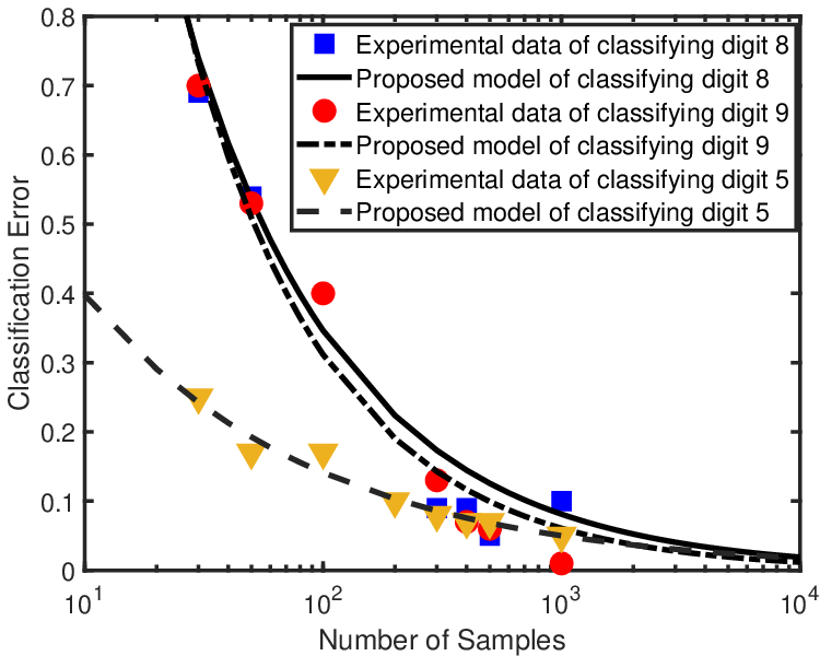
2) Approximation. This means that we can pre-train a large number of commonly-used models offline (not at the edge) and store their corresponding parameters of in a look-up table at the edge. Then by choosing a set of parameters from the table, the unknown error model at the edge can be approximated. This is because the error functions can share the same trend for two similar tasks, e.g., classifying digit ‘’ and ‘’ with SVM as shown in Fig. 3c. Notice that there may be a mismatch between the pre-training task and the real task at the edge. This is the case between classifying digit ‘’ and ‘’ in Fig. 3c. As a result, it is necessary to carefully measure the similarity between two tasks when choosing the parameters.
III-D Parameter Fitting of ResNet and PointNet
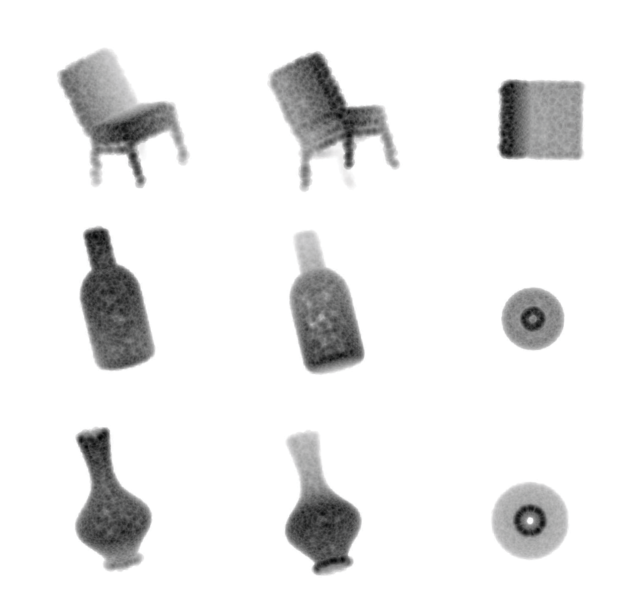
To verify the nonlinear model in (7) under deeper learning models and larger datasets, we train the -layer deep residual network (ResNet- with M parameters) [35] using the CIFAR-10 dataset as the input images, with training sample size ranging from to . The image in the CIFAR-10 dataset has pixels (each pixel has Bytes representing RGB), and each image sample has a size of . The training procedure is implemented with a diminishing learning rate and a mini-batch size of . After training for iterations ( hours), we test the trained model on a dataset with unseen samples, and obtain the corresponding classification error. It can be seen from Fig. 4a that the proposed model with matches the experimental data of ResNet- very well. Moreover, we also consider the PointNet (M parameters), which applies feature transformations and aggregates point features by max pooling [36, Fig. 2] to classify D point clouds dataset ModelNet40 (see examples in Fig. 4b). In ModelNet40, there are CAD models from object categories, split into for training and for testing. Each sample has points with three single-precision floating-point coordinates (Bytes), and the data size per sample is . After training for epochs ( hours) with a mini-batch of , the classification error versus the number of samples is obtained in Fig. 4a, and the proposed classification error model with matches the experimental data of PointNet very well.


IV MM-Based LCPA Algorithm
Based on the results in Section III, we can directly approximate the true error function by . However, to account for the approximation error between and (e.g., due to noise in samples or slight mismatch between data used for fitting and data observed in MTC devices), a weighting factor can be applied to , where a higher value of accounts for a larger approximation error.22 2 Since the real classification error is scattered around the fitted one, introducing means that we need to elevate the fitted curves to account for the possibilities that worse classification results may happen compared to our prediction. In other words, we should be more conservative (pessimistic) about our prediction. Then by replacing with and putting (4b) into to eliminate , problem becomes:
| (10a) | ||||
| (10b) | ||||
| (10c) | ||||
where constraints (10b)–(10c) come from equation (II) in the non-IID case and
| (11) |
It can be seen that is a nonlinear optimization problem due to the nonlinear classification error model (7). Moreover, the operator introduces non-smoothness to the problem, and the objective function is not differentiable. Thus the existing method based on gradient descent [18] is not applicable.
To solve , we propose to use the framework of MM [37, 38, 39, 40], which constructs a sequence of upper bounds on and replaces in with to obtain the surrogate problems. More specifically, given any feasible solution to , we define surrogate functions
| (12) |
and the following proposition can be established.
Proposition 1.
The functions satisfy the following conditions:
(i) Upper bound condition: .
(ii) Convexity: is convex in .
(iii) Local equality condition: and .
Proof.
See Appendix A. ∎
With part (i) of Proposition 1, an upper bound can be directly obtained if we replace the functions by around a feasible point. However, a tighter upper bound can be achieved if we treat the obtained solution as another feasible point and continue to construct the next-round surrogate function. In particular, assuming that the solution at the iteration is given by , the following problem is considered at the iteration:
| (13) |
Based on part (ii) of Proposition 1, the problem is convex and can be solved by off-the-shelf software packages (e.g., CVX Mosek [41]) for convex programming. Denoting its optimal solution as , we can set , and the process repeats with solving the problem . According to part (iii) of Proposition 1 and [37, Theorem 1], every limit point of the sequence is a KKT solution to as long as the starting point is feasible to (e.g., ). The entire procedure of the MM-based LCPA is summarized in the left hand branch of Fig. 4c.
In terms of computational complexity, involves primal variables and dual variables. The dual variables correspond to constraints in , where constraints come from the operator, constraints come from nonnegative power constraints, constraints come from the data-rate bounds, and one constraint comes from the power budget. Therefore, the worst-case complexity for solving is [42]. Consequently, the total complexity for solving is , where is the number of iterations needed for the algorithm to converge.
V Asymptotic Analysis and Insights to LCPA
To understand how LCPA works, this section investigates the asymptotic case when the number of antennas at the edge approaches infinity (i.e., ). Moreover, we consider the special case of and (i.e., each user group has only one unique user). For notational simplicity, we denote the unique user in group as user . As each task only involves one user, non-IID data distribution among users in a single task does not exist, and therefore constraints (10b)–(10c) can be removed. On the other hand, as , the channels from different users to the edge would be asymptotically orthogonal [43, 44, 45] and we have
| (14) |
Based on such orthogonality feature, and putting for into in , problem under and is rewritten as
| (15) |
where is a slack variable and has the interpretation of classification error level. The following proposition gives the optimal solution to .
Proposition 2.
The optimal to is
| (16) |
where satisfies .
Proof.
See Appendix B. ∎
To efficiently compute the classification error level , it is observed that the function is a decreasing function of . Therefore, the classification error level can be obtained from solving using bisection method within interval . More specifically, given and (initially and ), we set . If , we update ; otherwise, we update . This procedure is repeated until with . Since bisection method has a linear convergence rate [46], and in each iteration we need to compute scalar functions , the bisection method has a complexity of .
Scaling Law of Learning Centric Communication. According to Proposition 2, the user transmit power is inversely proportional to the wireless channel gain . On the other hand, it is exponentially dependent on the classification error level and the learning parameters . Moreover, among all parameters, is the most important factor, since is involved in both the power and exponential functions. The above observations disclose that in edge machine learning systems, the learning parameters will have more significant impacts on the radio resource allocation than those of the wireless channels.
Learning Centric versus Communication Centric Power Allocation. Notice that the result in (2) is fundamentally different from the most well-known resource allocation schemes (e.g., iterative water-filling [15] and max-min fairness [16]). For example, the water-filling solution for maximizing the system throughput under is given by
| (17) |
where is a constant chosen such that . On the other hand, the max-min fairness solution under is given by
| (18) |
It can be seen from (17) and (18) that the water-filling scheme would allocate more power resources to better channels, and the max-min fairness scheme would allocate more power resources to worse channels. But no matter which scheme we adopt, the only impact factor is the channel condition .
VI Large-scale Optimization under IID Datasets
Although a KKT solution to has been derived in Section IV, it can be seen that MM-based LCPA requires a cubic complexity with respect to . This leads to time-consuming computations if is in the range of hundreds or more. As a result, low-complexity large-scale optimization algorithms are indispensable. To this end, in this section we consider the case of under IID datasets, and develop an algorithm based on the FOM.
As , we put for into in , and the function is asymptotically equal to
| (19) |
Therefore, the problem in the case of IID datasets and is equivalent to
| (20) |
The major challenge for solving comes from the nonsmooth operator in the objective function, which hinders us from computing the gradients. To deal with the non-smoothness, we reformulate into a smooth bilevel optimization problem with -norm (simplex) constraints. Observing that the projection onto a simplex in Euclidean space requires high computational complexities, a mirror-prox LCPA method working on non-Euclidean manifold is proposed. In this way, the distance is measured by Kullback-Leibler (KL) divergence, and the non-Euclidean projection would have analytical expressions. Lastly, with an extragradient step, the proposed mirror-prox LCPA converges to the global optimal solution to with an iteration complexity of [47, 48, 49], where is the target solution accuracy.
More specifically, we first equivalently transform into a smooth bilevel optimization problem. By defining set and introducing variables such that , is rewritten as
| (21) |
It can be seen from that is differentiable with respect to either or , and the corresponding gradients are
| (22a) | ||||
| (22b) | ||||
where
| (23) |
with its element being
| (24) |
However, is a bilevel problem, with both the upper layer variable and the lower layer variable involved in the simplex constraints. In order to facilitate the projection onto simplex constraints, below we consider a non-Euclidean (Banach) space induced by -norm. In such a space, the Bregman distance between two vectors and is the KL divergence
| (25) |
and the following proposition can be established.
Proposition 3.
If the classification error is upper bounded by , then is –smooth in Banach space induced by -norm, where
| (26a) | ||||
| (26b) | ||||
with .
Proof.
See Appendix C. ∎
The smoothness result in Proposition 3 enables us to apply mirror descent (i.e., generalized gradient descent in non-Euclidean space) to and mirror ascent to in the -space [48]. This leads to the proposed mirror-prox LCPA, which is an iterative algorithm that involves i) a proximal step and ii) an extragradient step. In particular, the mirror-prox LCPA initially chooses a feasible and (e.g., and ). Denoting the solution at the iteration as , the following equations are used to update the next-round solution [48]:
| (27a) | ||||
| (27b) | ||||
| (27c) | ||||
| (27d) | ||||
where is the step-size, and the terms inside in (27a)–(27d) are obtained from (22a)–(22b). Notice that a small would lead to slow convergence of the algorithm while a large would cause the algorithm to diverge. According to [48], should be chosen inversely proportional to Lipschitz constant or derived in Proposition 3. In this paper, we set with , which empirically provides fast convergence of the algorithm.
How Mirror-prox LCPA Works. The formulas (27a)–(27b) update the variables along their gradient direction, while keeping the updated point close to the current point . This is achieved via the proximal operator that minimizes the distance (or ) plus a first-order linear function. Since the KL divergence is the Bregman distance, the update (27a)–(27b) is a Bregman proximal step. On the other hand, the gradients in (27c) and (27d) are computed using and , respectively. By doing so, we can obtain the look-ahead gradient at the intermediate point and for updating and . This “look-ahead” feature is called extragradient.
Lastly, we put the Bregman distance in (25), the function in (19), the gradient in (23), and a proper into (27a)–(27d). Based on the KKT conditions, the equations (27a)–(27b) are shown to be equivalent to
| (28a) | ||||
| (28b) | ||||
The equations (27c)–(27d) can be similarly reduced to closed-form expressions.
According to Proposition 3 and [47], the mirror-prox LCPA algorithm is guaranteed to converge to the optimal solution to . But in practice, we can terminate the iterative procedure when the norm is small enough, e.g., . The entire procedure for computing the solution to using the mirror-prox LCPA is summarized in the right hand branch of Fig. 4c. In terms of computational complexity, computing (28a) requires a complexity of . Since the number of iterations for the mirror-prox LCPA to converge is with being the target solution accuracy, the total complexity of mirror-prox LCPA would be .
VII Simulation Results and Discussions
This section provides simulation results to evaluate the performance of the proposed algorithms. It is assumed that the noise power (corresponding to power spectral density with bandwidth [27]), which includes thermal noise and receiver noise. The total transmit power at users is set to (i.e., ), with the communication bandwidth . The path loss of the user is adopted [40], and is generated according to [44]. Without otherwise specified, it is assumed that . We set and for all in Sections VII-A to VII-C. Simulations with upper and lower bounds on data amount will be presented in Section VII-D. Each point in the figures is obtained by averaging over simulation runs, with independent channels in each run. All optimization problems are solved by Matlab R2015b on a desktop with Intel Core i5-4570 CPU at 3.2 GHz and 8 GB RAM. All the classifiers are trained by Python 3.6 on a GPU server with Intel Core i7-6800 CPU at 3.4 GHz and GeForce GTX 1080 GPU.
VII-A CNN and SVM
We consider the aforementioned CNN and SVM classifiers with the number of learning models at the edge: i) Classification of MNIST dataset [30] via CNN; ii) Classification of digits dataset in Scikit-learn [34] via SVM. The data size of each sample is for the MNIST dataset and for the digits dataset in Scikit-learn. It is assumed that there are CNN samples and SVM samples in the historical dataset. The parameters in the two classification error models are assumed to be perfectly known and they are given by for CNN and for SVM as in Fig. 3b. Finally, it is assumed that since the approximation error of SVM in Fig. 3b is larger than that of CNN.
To begin with, the case of and with and is simulated. Under the above settings, we compute the collected sample sizes by executing the proposed MM-based LCPA, and the maximum error of classifiers (i.e., the worse classification result of CNN and SVM, where the classification error for each task is obtained from the machine learning experiment using the sample sizes from the power allocation algorithms) versus the total transmission time is shown in Fig. 5a. Besides the proposed MM-based LCPA, we also simulate two benchmark schemes: 1) Max-min fairness scheme [16, Sec. II-C]; 2) Sum-rate maximization scheme [17, Sec. IV]. It can be seen from Fig. 5a that the proposed MM-based LCPA algorithm with has a significantly smaller classification error compared to other schemes, and the gap concisely quantifies the benefit brought by more training images for CNN under joint communication and learning design. For example, at in Fig. 5a, the proposed MM-based LCPA collects MNIST images on average, while the sum-rate maximization and the max-min fairness schemes collect images and images, respectively. Furthermore, if we target at the same learning error, the proposed algorithm saves the transmission time by at least compared to benchmark schemes. This can be seen from Fig. 5a at the target error , where the proposed algorithm takes seconds for transmission, but other methods require about seconds. The saved time enables the edge to collect data for other edge computing tasks [50].


To get more insight into the edge learning system, the case of with and at is simulated, and the classification error versus the number of antennas is shown in Fig. 5b. It can be seen from Fig. 5b that the classification error decreases as the number of antennas increases, which demonstrates the advantage of employing massive MIMO in edge machine learning. More importantly, the proposed analytical solution in Proposition 2 outperforms the water-filling33 3 In the case of large , sum-rate maximization scheme [17, Sec. IV] would reduce to the iterative water-filling scheme [15], which allocates power according to (17). and max-min fairness schemes even at a relatively small number of antennas . This is achieved by allocating much more power resources to the first user (i.e., user uploading datasets for CNN), because training CNN is more difficult than training SVM. In particular, the transmit powers in are given by: 1) for the analytical LCPA scheme; 2) for the water-filling scheme; and 3) for the max-min fairness scheme. Notice that the performance gain brought by LCPA in Fig. 5b is slightly smaller than that in Fig. 5a, since the ratio is increased. But no matter what value and take, the proposed LCPA always outperforms existing algorithms due to its learning centric feature.
To verify the performance and the low complexity nature of the mirror-prox LCPA in Section VI when the number of antennas is large, the case of and at is simulated, with containing the first users and containing the rest users. The maximum error of classifiers versus the number of users is shown in Fig. 5c. It can be seen that the proposed mirror-prox LCPA algorithm significantly reduces the classification error compared to the water-filling and max-min fairness schemes, and it achieves performance close to that of the MM-based LCPA. On the other hand, the average execution time at is given by: 1) for the MM-based LCPA; 2) for the mirror-prox LCPA; 3) for the water-filling scheme; and 4) for the max-min fairness scheme. Compared with MM-based LCPA, the mirror-prox LCPA saves at least of the computation time, which corroborates the linear complexity derived in Section VI.
VII-B Deep Neural Networks
Next, we consider the ResNet- as task and the CNN in Section III as task at the edge, with and . The error rate parameters are given by and . In addition, it is assumed that , , and there is no historical sample at the edge (i.e., ). We simulate the case of and with and . For ResNet-, we assume that the datasets are formed by dividing the CIFAR-10 dataset into two parts, each with different samples. For CNN, we assume that the datasets are formed by dividing the MNIST dataset into two parts, each also with different samples. The worse classification error between the two tasks (obtained from the machine learning experiment using the sample sizes from the power allocation algorithms) is: 1) for MM-based LCPA; 2) for the sum-rate maximization scheme; and 3) for the max-min fairness scheme. It can be seen that the proposed LCPA achieves the smallest classification error, which demonstrates the effectiveness of learning centric resource allocation under deep neural networks and large datasets.


VII-C Practical Considerations
In Sections VII-A and VII-B, we have assumed that the parameters are perfectly known. In practice, we need to estimate them from the historical data. More specifically, denote the historical data as . We take of the historical data in as the training dataset , and the remaining as the validation dataset for all . Therefore, the number of training samples for estimating is . Based on the above dataset partitioning, the parameters are estimated in two stages:
- •
In the training stage, we can vary the sample size as within . For each , we train the learning model for epochs and test the trained model on the validation dataset . The classification errors corresponding to the different sample sizes are given by .
- •
In the fitting stage, with the classification error versus sample size, the parameters in are found via the nonlinear least squares fitting in (9).
Assuming that the complexity of processing each image (e.g., for CNN, each processing stage includes a backward pass and a forward pass) is where is the number of parameters in the learning model, the complexity in the training stage is . If is smaller than the total number of samples after data collection, then would be smaller than the actual model training complexity. On the other hand, the complexity in the fitting stage is negligible, since the problem (9) only has two variables. Even using a naive brute-force search with a step size of for each dimension, the running time for solving (9) is only seconds on a desktop with Intel Core i5-4570 CPU at 3.2 GHz and 8 GB RAM.
To illustrate the above procedure, we consider the case of and with , where the first task is to train the CNN with user and the second task is to train the SVM with users . For CNN, we assume that the dataset contains different samples from the MINST dataset. For SVM, we assume that the datasets are formed by dividing the scikit-learn digit dataset into four parts, each with different samples. To conform with the size of , the datasets are augmented by appending samples (generated via random rotations of the original samples) to the original samples. The test dataset for CNN contains another samples from the MNIST dataset and the test dataset for SVM contains another samples from the scikit-learn digits dataset. It is assumed that and . According to the “-training and -validation” partitioning of , we have and , meaning that there are and historical samples for training CNN and SVM, respectively. For CNN, we vary the sample size as and perform training for epochs. The classification errors on the validation dataset are given by , and after model fitting we have . On the other hand, for SVM, we vary the sample size as . The classification errors on the validation dataset are given by , and after model fitting we have .
Based on the above estimation results for , the classification errors at for different schemes are compared in Fig. 6a. It can be seen from Fig. 6a that the proposed LCPA reduces the minimum classification error by at least compared with other simulated schemes. To demonstrate the performance of the proposed LCPA under various values of , the classification error versus at is shown in Fig. 6b. It can be seen from Fig. 6b that the classification error increases as decreases, which is due to the loss of samples during wireless transmission. However, no matter what value takes, the proposed LCPA achieves the minimum classification error among all the simulated schemes.
VII-D Non-IID Dataset
In the non-IID case, we add one more user (denoted as user 6) to the system considered in Section VII-C, with the first task training the CNN with users and the second task training the SVM with users . The dataset repeats the first sample in the MINST dataset for times and . Out of this , we use as the training dataset and as the validation dataset . We train the CNN in Fig. 1 using the training dataset for epochs, and obtain the parameter in the CNN. We then compute the prediction confidence for all the data based on equation (6) with the probability function being the softmax output of CNN. It turns out that the least confident samples in and have the following scores: and . For user , since the CNN model is not sure about its prediction, we set and . For user , since the CNN model can predict its validation data with very high confidence, we set and . Based on the ratio between and , we use samples from and samples from for estimating . Then we have . For the SVM model, since the data from users are assumed to be IID, is the same as that in Section VII-C, i.e., .
The comparison of classification error in the non-IID case is shown in Fig. 6c. It can be seen from Fig. 6c that the performance of MM-based LCPA (without uncertainty sampling) becomes worse than that in Fig. 6a, which is due to the additional resources allocated to user . However, the proposed MM-based LCPA still outperforms the sum-rate maximization and max-min fairness schemes. More importantly, by adopting the uncertainty sampling method to distinguish the users’ data quality, the classification error of LCPA can be further reduced (e.g., from the black bar to the yellow bar in Fig. 6c). This demonstrates the benefit brought by joint estimation of sample size and prediction confidence in edge machine learning systems.
VIII Conclusions
This paper has introduced the LCPA concept to edge machine learning. By adopting an empirical classification error model, learning efficient edge resource allocation has been obtained via the MM-based LCPA algorithm. In the large-scale settings, a fast FOM has been derived to tackle the curse of high-dimensionality. Simulation results have shown that the proposed LCPA algorithms achieve lower classification errors than existing power allocation schemes. Furthermore, the proposed fast algorithm significantly reduces the execution time compared with the MM-based LCPA while still achieving satisfactory performance.
Appendix A Proof of Proposition 1
To prove part (i), consider the following inequality:
| (29) |
which is obtained from for any due to the convexity of . Adding on both sides of (29), we obtain
| (30) |
Putting the result of (30) into in (12) and since is a decreasing function of , we immediately prove
| (31) |
To prove part (ii), we first notice that is a composition function of , where and
| (32) |
Since and , the function is convex and nonincreasing. Adding to the fact that is a concave function of , we immediately prove the convexity of using the composition rule [41, Ch. 3, pp. 84].
Finally, to prove and , we put into the functions , and we immediately obtain part (iii).
Appendix B Proof of Proposition 2
To prove this proposition, the Lagrangian of is
| (33) |
where are non-negative Lagrange multipliers. According to the KKT conditions and [41], the optimal must together satisfy
| (34) |
where
| (35) |
with ( if ). Notice that holds for any . Based on the result of (34), it is clear that . Adding to the fact that and , we must have . Now we will consider two cases.
- •
. In this case, must hold.
- •
. In such a case, based on the complementary slackness condition, we must have . Putting into (34) and using , holds. Using and the complementary slackness condition, for all .
Combining the above two cases gives (2) and the proposition is proved.
Appendix C Proof of Proposition 3
To prove this proposition, we need the following lemma for .
Lemma 1.
If , the gradient function satisfies the following:
(i) ;
(ii) .
Proof.
To begin with, the assumption gives
| (36) |
Based on (36) and the expression of in (24), we have
| (37) |
where the second inequality is due to . Putting the above result into (23), and based on the definition of in (26b), part (i) is immediately proved.
Next, to prove part (ii), we notice that the derivative in (24) can be rewritten as , with the auxiliary functions
| (38a) | ||||
| (38b) | ||||
Using the result in (36) and due to , we have
| (39) |
Furthermore, according to Lipschitz conditions [48] of and , they satisfy
| (40a) | ||||
| (40b) | ||||
As a result, the following inequality is obtained:
| (41) |
where the first inequality is due to , and the second inequality is obtained from (39) and (40a)–(40b). By taking the maximum of (41) for all , part (ii) is proved. ∎
Based on Lemma 1, we are now ready to prove the proposition. In particular, according to [47, 48, 49], the function is –smooth if and only if
| (42a) | ||||
| (42b) | ||||
| (42c) | ||||
| (42d) | ||||
for any and . To prove the above inequalities, we need to upper bound the left hand sides of (42a)–(42d) and compare the bounds with the right hand sides of (42a)–(42d). To this end, the left hand side of (42a) is bounded as
| (43) |
where the last inequality is from Lemma 1. Further due to , the equation (42a) is proved. On the other hand, the left hand side of (42b) is upper bounded as
| (44) |
where the last inequality is from Lemma 1. In addition, the left hand side of (42c) can be upper bounded as
| (45) |
Finally, since the left hand side of (42d) is zero, we immediately have that (42d) holds.
References
- [1] V. Vapnik, The Nature of Statistical Learning Theory, Springer, New York, 1998.
- [2] Y. LeCun, Y. Bengio, and G. Hinton, “Deep learning,” Nature, vol. 521, pp. 436–444, May 2015.
- [3] M. Stolpe, “The Internet of Things: Opportunities and challenges for distributed data analysis,” ACM SIGKDD Explorations Newsletter, vol. 18, no. 1, pp. 15–34, Jun. 2016.
- [4] H. Li, K. Ota, and M. Dong, “Learning IoT in edge: Deep learning for the Internet of Things with edge computing,” IEEE Netw., vol. 32, no. 1, pp. 96–101, Feb. 2018.
- [5] G. Zhu, D. Liu, Y. Du, C. You, J. Zhang, and K. Huang, “Toward an Intelligent Edge: Wireless Communication Meets Machine Learning,” IEEE Commun. Mag., vol. 58, no. 1, pp. 19–25, Jan. 2020.
- [6] J. Park, S. Samarakoon, M. Bennis, and M. Debbah, “Wireless network intelligence at the edge,” Proc. IEEE, vol. 107, no. 11, pp. 2204–2239, Nov. 2019.
- [7] Z. Zhou, X. Chen, E. Li, L. Zeng, K. Luo, and J. Zhang, “Edge intelligence: Paving the last mile of artificial intelligence with edge computing,” Proc. IEEE, vol. 107, no. 8, pp. 1738–1762, Aug. 2019.
- [8] H. B. McMahan, E. Moore, D. Ramage, S. Hampson, and B. Arcas, “Communication-efficient learning of deep networks from decentralized data,” in Proc. AISTATS, Fort Lauderdale, FL, Apr. 2017.
- [9] S. Wang, T. Tuor, T. Salonidis, K. K. Leung, C. Makaya, T. He, and K. Chan, “Adaptive federated learning in resource constrained edge computing systems,” IEEE J. Sel. Areas Commun., vol. 37, no. 6, pp. 1205–1221, Jun. 2019.
- [10] D. Gündüz, P. de Kerret, N. D. Sidiropoulos, D. Gesbert, C. Murthy, and M. van der Schaar, “Machine learning in the air,” IEEE J. Sel. Areas Commun., vol. 37, no. 10, pp. 2184–2199, Oct. 2019.
- [11] C. Zhang, P. Patras, and H. Haddadi, “Deep learning in mobile and wireless networking: A survey,” IEEE Commun. Surveys Tuts., vol. 21, no. 3, pp. 2224–2287, Thirdquarter, 2019.
- [12] F. Tariq, M. R. A. Khandaker, K.-K. Wong, M. Imran, M. Bennis, and M. Debbah, “A speculative study on 6G,” 2019. [Online]. Available: https://arxiv.org/abs/1902.06700
- [13] W. Saad, M. Bennis, and M. Chen, “A vision of 6G wireless systems: Applications, trends, technologies, and open research problems,” IEEE Netw., vol. 34, no. 3, pp. 134–142, May/Jun. 2020.
- [14] K. B. Letaief, W. Chen, Y. Shi, J. Zhang, and Y.-J. A. Zhang, “The roadmap to 6G–AI empowered wireless networks,” IEEE Commun. Mag., vol. 57, no. 8, pp. 84–90, Aug. 2019.
- [15] W. Yu, W. Rhee, S. Boyd, and J. M. Cioffi, “Iterative water-filling for Gaussian vector multiple-access channels,” IEEE Trans. Inf. Theory, vol. 50, no. 1, pp. 145–152, Jan. 2004.
- [16] M. Schubert and H. Boche, “Solution of the multiuser downlink beamforming problem with individual SINR constraints,” IEEE Trans. Veh. Technol., vol. 53, no. 1, pp. 18–28, Jan. 2004.
- [17] H. Al-Shatri and T. Weber, “Achieving the maximum sum rate using D.C. programming in cellular networks,” IEEE Trans. Signal Process., vol. 60, no. 3, pp. 1331–1341, Mar. 2012.
- [18] A. Beck, A. Nedić, A. Ozdaglar, and M. Teboulle, “An gradient method for network resource allocation problems,” IEEE Trans. Control Netw. Syst., vol. 1, no. 1, pp. 64–73, Mar. 2014.
- [19] S. Geman, E. Bienenstock, and R. Doursat, “Neural networks and the bias/variance dilemma,” Neural Comput., vol. 4, no. 1, pp. 1–58, 1992.
- [20] P. Domingos, “A unified bias-variance decomposition and its applications,” in Proc. ICML, Stanford, CA, USA, 2000, pp. 231–238.
- [21] M. Johnson, P. Anderson, M. Dras, and M. Steedman, “Predicting classification error on large datasets from smaller pilot data,” in Proc. ACL, Melbourne, Australia, Jul. 2018, pp. 450–455.
- [22] P. Kolachina, N. Cancedda, M. Dymetman, and S. Venkatapathy, “Prediction of learning curves in machine translation,” in Proc. ACL, Jeju Island, Korea, 2012, pp. 22–30.
- [23] I. Y. Chen, F. D. Johansson, and D. Sontag, “Why is my classifier discriminatory?” in Proc. NIPS, Montréal, Canada, 2018, pp. 3543–3554.
- [24] H. S. Seung, H. Sompolinsky, and N. Tishby, “Statistical mechanics of learning from examples,” Phys. Rev. A, vol. 45, pp. 6056–6091, Apr. 1992.
- [25] D. Yarowsky, “Unsupervised word sense disambiguation rivaling supervised methods,” in Proc. ACL, Stroudsburg, PA, 1995, pp. 189–196.
- [26] I. Radosavovic, P. Dollaŕ, R. Girshick, G. Gkioxari, and K. He, “Data distillation: Towards omni-supervised learning,” in Proc. CVPR, 2018, pp. 4119–4128.
- [27] 3GPP, “Performance requirements for narrowband IoT,” LTE; Evolved Universal Terrestrial Radio Access (E-UTRA); Base Station (BS) Radio Transmission and Reception, TS 36.104 version 15.3.0 Release 15, Jul. 2018.
- [28] Y. Xiao, Y. Jia, C. Liu, X. Cheng, J. Yu, and W. Lv, “Edge computing security: State of the art and challenges,” Proc. IEEE, vol. 107, no. 8, pp. 1608–1631, Aug. 2019.
- [29] K. Zheng, H. Meng, P. Chatzimisios, L. Lei, and X. Shen, “An SMDP-based resource allocation in vehicular cloud computing systems,” IEEE Trans. Ind. Electron., vol. 62, no. 12, pp. 7920–7928, Dec. 2015.
- [30] L. Deng, “The MNIST database of handwritten digit images for machine learning research,” IEEE Signal Process. Mag., vol. 29, no. 6, pp. 141–142, Nov. 2012.
- [31] 3GPP, 5G; NR; Physical Layer Procedures for Control, TS 38.213 version 15.5.0 Release 15, May 2019.
- [32] M. Chen, Z. Yang, W. Saad, C. Yin, H. V. Poor, and S. Cui, “A joint learning and communications framework for federated learning over wireless networks,” 2019. [Online]. Available: https://arxiv.org/pdf/1909.07972.pdf
- [33] B. Settles, “Active Learning Literature Survey,” Computer Sciences Technical Report 1648, University of Wisconsin-Madison, Jan. 2009.
- [34] F. Pedregosa, G. Varoquaux, A. Gramfort, et al., “Scikit-learn: Machine learning in Python,” J. Mach. Learn. Res., vol. 12, pp. 2825–2830, Oct. 2011.
- [35] K. He, X. Zhang, S. Ren, and J. Sun, “Deep residual learning for image recognition,” in Proc. CVPR, Las Vegas, Nevada, 2016, pp. 770–778.
- [36] C. R. Qi, H. Su, K. Mo, and L. J. Guibas, “Pointnet: Deep learning on point sets for 3D classification and segmentation,” in Proc. CVPR, Honolulu, Hawaii, 2017, pp. 652–660.
- [37] B. R. Marks and G. P. Wright, “A general inner approximation algorithm for nonconvex mathematical programs,” Oper. Res., vol. 26, no. 4, Jul. 1978.
- [38] T. Lipp and S. Boyd, “Variations and extensions of the convex-concave procedure,” Optim. Eng., vol. 17, no. 2, pp. 263-287, Jun. 2016.
- [39] Y. Sun, P. Babu, and D. P. Palomar, “Majorization-minimization algorithms in signal processing, communications, and machine learning,” IEEE Trans. Signal Process., vol. 65, no. 3, pp. 794–816, Feb. 2017.
- [40] S. Wang, M. Xia, K. Huang, and Y.-C. Wu, “Wirelessly powered two-way communication with nonlinear energy harvesting model: Rate regions under fixed and mobile relay,” IEEE Trans. Wireless Commun., vol. 16, no. 12, pp. 8190–8204, Dec. 2017.
- [41] S. Boyd and L. Vandenberghe, Convex Optimization. Cambridge, U.K.: Cambridge Univ. Press, 2004.
- [42] A. Ben-Tal and A. Nemirovski, Lectures on Modern Convex Optimization (MPS/SIAM Series on Optimizations), Philadelphia, PA, USA: SIAM, 2013.
- [43] L. Lu, G. Y. Li, A. L. Swindlehurst, A. Ashikhmin, and R. Zhang, “An overview of massive MIMO: Benefits and challenges,” IEEE J. Sel. Topics Signal Process., vol. 8, no. 5, pp. 742–758, Oct. 2014.
- [44] H. Q. Ngo, E. G. Larsson, and T. L. Marzetta, “Energy and spectral efficiency of very large multiuser MIMO systems,” IEEE Trans. Commun., vol. 61, no. 4, pp. 1436–1449, Apr. 2013.
- [45] L. Liu and W. Yu, “Massive connectivity with massive MIMO Part I: Device activity detection and channel estimation,” IEEE Trans. Signal Process., vol. 66, no. 11, pp. 2933–2946, Jun. 2018.
- [46] K. E. Atkinson, An Introduction to Numerical Analysis (2nd edition), New York: John Wiley and Sons, 1989.
- [47] A. Nemirovski, “Prox-method with rate of convergence for variational inequalities with Lipschitz continuous monotone operators and smooth convex-concave saddle point problems,” SIAM J. Optimiz., vol. 15, no. 1, pp. 229–251, 2004.
- [48] S. Bubeck, “Convex optimization: Algorithms and complexity,” Found. Trends Mach. Learn., vol. 8, no. 3-4, pp. 231–357, Nov. 2015.
- [49] A. Konar and N. D. Sidiropoulos, “Fast approximation algorithms for a class of non-convex QCQP problems using first-order methods,” IEEE Trans. Signal Process., vol. 65, no. 13, pp. 3494–3509, Jul. 2017.
- [50] S. Yu, B. Dab, Z. Movahedi, R. Langar, and L. Wang, “A socially-aware hybrid computation offloading framework for multi-access edge computing,” IEEE Trans. Mobile Comput., vol. 19, no. 6, pp. 1247–1259, Jun. 2020.