跳到论文正文
W Papers独立论文阅读器 arXiv:1911.04906 论文正文 计算阅读时间 · 0%
引用这篇论文根据当前论文元数据生成,正式投稿前建议核对。


License: arXiv.org perpetual non-exclusive license
arXiv:1911.04906v2 [quant-ph] 27 Feb 2020

Coding closed and open quantum systems in MATLAB: applications in quantum optics and condensed matter

Ariel Norambuena    Diego Tancara Affiliation:  Faculty of Physics, Pontificia Universidad Católica de Chile, Avda. Vicuña Mackenna 4860, Santiago, Chile       Raúl Coto Email: ariel.norambuena@umayor.cl
Abstract

We develop a package of numerical simulations implemented in MATLAB to solve complex many-body quantum systems. We focus on widely used examples that include the calculation of the magnetization dynamics for the closed and open Ising model, dynamical quantum phase transition in cavity QED arrays, Markovian dynamics for interacting two-level systems, and the non-Markovian dynamics of the pure-dephasing spin-boson model. These examples will be useful for undergraduate and graduate students with a medium or high background in MATLAB, and also for researches interested in numerical studies applied to quantum optics and condensed matter systems.

1 Introduction

Myriad current research fields in quantum optics and condensed matter demand numerical analysis of complex many-body systems (MBS). Interesting effects like dynamical quantum phase transition (DQPT), meta-stability, steady states, among others, can naturally emerge in MBS. These effects are observed in closed decoherence-free dynamics such as the Jaynes-Cummings [1], Jaynes-Cummings-Hubbard [2], trapped ions [3], cavity opto-mechanics [4] or Ising models [5]. Furthermore, for open quantum systems, the environment may cause memory effects in the reservoir time scale, which is known as non-Markovianity (NM) [6, 7]. From the theory of open quantum systems, NM can be described either by a time-local convolutionless or a convolution master equation [8]. In most of these cases, it is highly demanding to handle these kinds of problems with analytical tools, and a numerical approach can appear as the only solution. For instance, this is the case for systems with non-trivial system-environment interactions [9] and quantum systems with many degrees of freedom.

Nowadays, numerical toolboxes or open-source packages allow saving time when dealing with analytically untreatable problems, without the requirement of a vast knowledge in computational physics. Toward this end, we found the Wave Packet open-source package of MATLAB [10, 11, 12], the tutorial Doing Physics with MATLAB [13], the introductory book Quantum Mechanics with MATLAB [14], and the Quantum Optics Toolbox of MATLAB [15]. However, most of them does not have examples illustrating many-body effects in both closed and open quantum systems. In this work, we provide several examples implemented in MATLAB to code both closed and open dynamics in many-body systems. This material will be useful for undergraduate and graduate students, either master or even doctoral courses. More importantly, the advantage of using the matrix operations in MATLAB can be crucial to work with Fock states, spin systems, or atoms coupled to light.

MATLAB is a multi-paradigm computational language that provides a robust framework for numerical computing based on matrix operations [16], along with a friendly coding and high performance calculations. Hence, the solutions that we provide have a pedagogical impact on the way that Quantum Mechanical problems can be efficiently tackle down. This paper is organized as follows. In section 2 we introduce the calculation of observables for a decoherence-free closed quantum many-body systems. We discuss the transverse Ising and the Jaynes-Cumming-Hubbard models with a particular interest in dynamical quantum phase transitions. In Section 3, we model the Markovian and non-Markovian dynamics of open quantum systems using the density matrix. The dissipative dynamics of interacting two-level systems is calculated using a fast algorithm based on eigenvalues and eigenmatrices. Finally, the non-Markovian dynamics of the pure-dephasing spin-boson model is discussed and modelled for different spectral density functions, in terms of a convolutionless master equation.

2 Closed quantum systems

In the framework of closed quantum many-body systems the dynamics is ruled by time-dependent Shcrödinger equation [17]

i​ℏ​d​|Ψ⁡(t)⟩d​t=H^​|Ψ⁡(t)⟩,i\hbar{d|\Psi(t)\rangle\over dt}=\hat{H}|\Psi(t)\rangle, (1)

where |Ψ⁡(t)⟩|\Psi(t)\rangle and H^\hat{H} are the many-body wavefunction and Hamiltonian of the system, respectively. For a time-independent Hamiltonian, the formal solution for the wavefunction reads

|Ψ(t)⟩=U^(t)|Ψ(0)⟩=e−iH^t/ℏ|Ψ(0)⟩,|\Psi(t)\rangle=\hat{U}(t)|\Psi(0)\rangle=e^{-i\hat{H}t/\hbar}|\Psi(0)\rangle, (2)

where U^(t)=exp(−iH^t/ℏ)\hat{U}(t)=\mbox{exp}(-i\hat{H}t/\hbar) is the time propagator operator. The numerical implementation of this type of dynamics relies on the construction of the initial state |Ψ⁡(0)⟩|\Psi(0)\rangle (vector), the time propagator U^​(t)\hat{U}(t) (matrix), and the system Hamiltonian H^\hat{H} (matrix). For illustration, we introduce first two spin-1/21/2 particles described by the following Hamiltonian

H^spins=−J​S1x​S2x−B⁡(S1x+S2x).\hat{H}_{\rm spins}=-JS_{1}^{x}S_{2}^{x}-B(S_{1}^{x}+S_{2}^{x}). (3)

In MATLAB, the above Hamiltonian can be coded as follow (using J=1J=1 and B=0.1​JB=0.1J)

1 J = 1; % Value of the coupling J
2 B = 0.1*J; % Value of the magnetic field
3 Sx = [0 1;1 0]; % S_x operator
4 Sz = [1 0; 0 -1]; % S_z operator
5 I = eye(2); % Identity matrix
6 Hspins = -J*kron(Sx,Sx)-B*(kron(Sx,I)+kron(I,Sx)); % Hamiltonian

where eye(2) generates the 2×22\times 2 identity matrix and kron(XX,YY) = X⊗YX\otimes Y gives the tensor product of matrices XX and YY. Now, we illustrate how to solve the spin dynamics for the initial condition |Ψ⁡(0)⟩=|↓⟩1⊗|↓⟩2|\Psi(0)\rangle=\ket{\downarrow}_{1}\otimes\ket{\downarrow}_{2} from the initial time ti=0t_{i}=0 to the final time tf=2​Tt_{f}=2T with T=2​π/(2​B)T=2\pi/(2B). We must point out that the method we will use next is not valid for time-dependent Hamiltonians. For completeness, we compute the average magnetization along the α\alpha direction, which is defined as

⟨Mα⟩=1N∑i=1N⟨Ψ(t)|Siα|Ψ(t)⟩,α=x,y,z,\langle M_{\alpha}\rangle={1\over N}\sum_{i=1}^{N}\langle\Psi(t)|S_{i}^{\alpha}|\Psi(t)\rangle,\quad\alpha=x,y,z, (4)

where NN is the number of spins and |Ψ⁡(t)⟩|\Psi(t)\rangle is the many-body wavefunction given in equation (2). In our particular case, N=2N=2, and thus we can write the following code to compute ⟨Mz⟩\langle M_{z}\rangle
1 down = [0 1]'; % Quantum state down = [0 1]^T
2 Psi_0 = kron(down,down); % Initial wavefunction
3 T = 2*pi/(2*B); % Period of time
4 Nt = 1000; % Number of steps to construct time vector
5 ti = 0; % Initial time
6 tf = 2*T; % Final time
7 dt = (tf-ti)/(Nt-1); % Step time dt
8 t = ti:dt:tf; % Time vector
9 U = expm(-1i*Hspins*dt); % Time propagator operator U(dt)
10 SSz = (kron(Sz,I)+kron(I,Sz))/2; % Operator S1^z + S2^z
11 Mz = zeros(size(t)); % Average magnetization
12 for n=1:length(t) % Iteration to find Psi(t) and Mz(t)
13 if n==1
14 Psi = Psi_0; % Initial wavefunction
15 else
16 Psi = U*Psi; % Wavefuntion at time t_n
17 end
18 Mz(n) = Psi'*SSz*Psi; % Average magnetization at time t_n
19 end
20 plot(t/T,real(Mz),'r-','LineWidth',3)
21 xlabel('$t/T$','Interpreter','LaTex','Fontsize', 30)
22 ylabel('$\langle M_z \rangle$','Interpreter','LaTex','Fontsize', 30)
23 set(gca,'fontsize',21)

Refer to caption

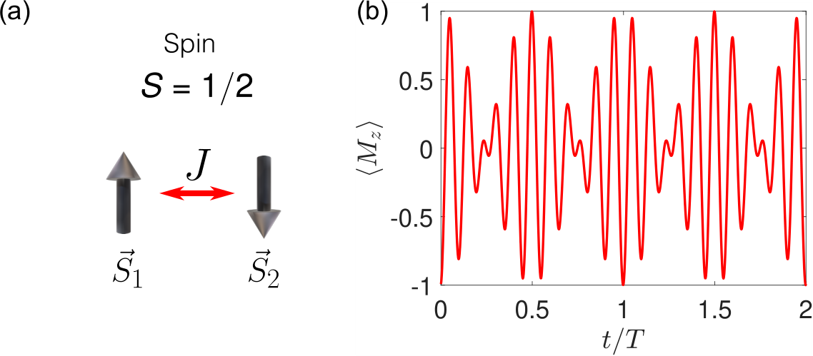
Figure 1: (a) Schematic representation of the two-spin system. (b) Average magnetization along the zz direction for J=1J=1 and B=J/10B=J/10 and considering the initial condition|Ψ⁡(0)⟩=|↓⟩1⊗|↓⟩2|\Psi(0)\rangle=\ket{\downarrow}_{1}\otimes\ket{\downarrow}_{2}. The time is divided by the natural period T=2​π/(2​B).T=2\pi/(2B).

By carefully looking at our code, we observed that MATLAB provides an intuitive platform to simulate quantum dynamics. First, the Hamiltonian defined in equation (3) can be easily implemented if operators (matrices SixS_{i}^{x}) are defined, and the two-body interaction is written using the kron() function. The tensor product defined as kron() reconstructs the Hilbert space of the system (two spin-1/2 particles). Second, the time evolution only depends on the initial state (vector Psi_0) and the time propagator U = expm(-1i*H*dt), where dt is the time step. We remark that it is convenient to use the expm() function of MATLAB to calculate the exponential of a matrix. Finally, the for loop allows us to actualize the wavefunction |Ψ⁡(t)⟩|\Psi(t)\rangle at every time using the recursive relation Psi = U*Psi (Ψn+1=U​Ψn\Psi_{n+1}=U\Psi_{n}), where the term of the left hand is the wavefunction at time tn+1=tn+d​tt_{n+1}=t_{n}+dt. To have numerical stability is necessary to satisfy the condition d​t≪ℏ/max⁡(|H^|)dt\ll\hbar/\max(|\hat{H}|). Hence, using the wavefunction we can calculate the average magnetization ⟨Mz⟩=⟨Ψ⁡(t)|Mz|Ψ⁡(t)⟩\langle M_{z}\rangle=\langle\Psi(t)|M_{z}|\Psi(t)\rangle employing the command Mz(n) = Psi’*SSz*Psi.

In figure 1 we plotted the expected average magnetization ⟨Mz⟩\langle M_{z}\rangle for the two-spin system. Initially, the system has a magnetization ⟨Mz⟩=−1\langle M_{z}\rangle=-1 due to the condition |Ψ⁡(0)⟩=|↓⟩1⊗|↓⟩2|\Psi(0)\rangle=\ket{\downarrow}_{1}\otimes\ket{\downarrow}_{2}, and then two characteristic oscillations are observed. The slow and fast oscillations in the signal correspond to the influence of BB and JJ, respectively.

We remark that this example does not require any additional package to efficiently run the codes. In the following, all codes may be executed using the available MATLAB library and the functions introduced in each example. In the next subsection, we introduce three relevant many-body problems, namely the transverse Ising, the Rabi-Hubbard and the Jaynes-Cummings-Hubbard models. For each case we write down an algorithm to solve the many-body dynamics.

2.1 Ising model

Let us consider the following transverse Ising Hamiltonian [3]

H^Ising=H1+H0=−∑i≠jNJi​jS^ixS^jx−B∑i=1NS^iz,\hat{H}_{\rm Ising}=H_{1}+H_{0}=-\sum_{i\neq j}^{N}J_{ij}\hat{S}_{i}^{x}\hat{S}_{j}^{x}-B\sum_{i=1}^{N}\hat{S}_{i}^{z}, (5)

where Ji​jJ_{ij} is the coupling matrix, BB is the external magnetic field, and NN is the number of spins. The spin operators S^iα\hat{S}_{i}^{\alpha} with α=x,y,z\alpha=x,y,z and i=1,…,Ni=1,...,N are the Pauli matrices for S=1/2S=1/2.

It is important to analyse the required memory to simulate the dynamics of the Ising model. The dimension of the Hilbert space for NN spin-1/2 particles is dimH=2N\mbox{dim}_{H}=2^{N}, and considering that a double variable requires 8 bytes we found that the memory required (in GB) is given by the expression dimH2×8×10−9\mbox{dim}_{H}^{2}\times 8\times 10^{-9}. The scaling ∝dimH2\propto\mbox{dim}_{H}^{2} is due to the Hermitian matrix structure of the Hamiltonian. For instance, to simulate 14 spins, we need at least 2.2 GB of memory. In what follows, the reader must check the computational cost of each example.

The interaction between adjacent spins is modelled using Ji​j=|i−j|−α/JJ_{ij}=|i-j|^{-\alpha}/J, where α≥0\alpha\geq 0 and J=(N−1)−1​∑i>jJi​jJ=(N-1)^{-1}\sum_{i>j}J_{ij} [18, 19]. We set B=J/0.42B=J/0.42 as it was recently used in Ref [20] to study dynamical phase transition in trapped ions. The ground state of the Hamiltonian H1H_{1} has a double degeneracy given by H1​|Ψη⟩=Eη​|Ψη⟩H_{1}|\Psi_{\eta}\rangle=E_{\eta}|\Psi_{\eta}\rangle, where |Ψ→⟩|\Psi_{\rightarrow}\rangle and |Ψ←⟩|\Psi_{\leftarrow}\rangle are the degenerate ground states and E←=E→E_{\leftarrow}=E_{\rightarrow} the corresponding energies. To study the dynamical quantum phase transition of this system we introduce the following rate function Λ⁡(t)\Lambda(t) [20]

Λ⁡(t)=minη=→,←⁡[−N−1​ln⁡(Pη​(t))],\Lambda(t)=\min_{\eta=\rightarrow,\leftarrow}\left[-N^{-1}\ln(P_{\eta}(t))\right], (6)

where Pη​(t)=|⟨Ψη|Ψ⁡(t)⟩|2P_{\eta}(t)=|\langle\Psi_{\eta}|\Psi(t)\rangle|^{2} is the probability to return to the ground state being |Ψ⁡(t)⟩=exp​(−i​H^Ising​t)​|Ψ⁡(0)⟩|\Psi(t)\rangle=\mbox{exp}(-i\hat{H}_{\rm Ising}t)|\Psi(0)\rangle (ℏ=1\hbar=1). To compute the magnetization vector along the xx direction we use equation (4) with α=x\alpha=x. The explicit code in MATLAB is showed below

1 Nspins = 6; % Number of spins
2 H0 = zeros(2^Nspins,2^Nspins);
3 H1 = zeros(2^Nspins,2^Nspins);
4 J = 0;
5 alpha = 0.2; % Parameter \alpha
6 for j=1:Nspins
7 for i=j+1:Nspins
8 Jij = abs(i-j)^(-alpha);
9 J = J + (Nspins-1)^(-1)*Jij;
10 end
11 end
12 B = J/0.42; % Magnetic field
13 Sx = [0 1;1 0];
14 Sz = [1 0;0 -1];
15 for i=1:Nspins
16 Szi = getSci(Sz,i,Nspins);
17 H0 = H0 - B*Szi; % Hamiltonian for the magnetic field
18 for j=1:Nspins
19 if i~=j
20 Sxi = getSci(Sx,i,Nspins);
21 Sxj = getSci(Sx,j,Nspins);
22 Vij = abs(i-j)^(-alpha)/J;
23 H1 = H1 - Vij*Sxi*Sxj; % Interaction Hamiltonian
24 end
25 end
26 end
27 H = H0 + H1; % Total hamiltonian
28 xr = [1 1]'/sqrt(2); % Single-particle state |Psi_{-->}>
29 xl = [-1 1]'/sqrt(2); % Single-particle state |Psi_{<--}>
30 Xr = xr;
31 Xl = xl;
32 for n=1:Nspins-1
33 Xr = kron(Xr,xr); % Many-body state |Psi_{-->}>
34 Xl = kron(Xl,xl); % Many-body state |Psi_{<--}>
35 end
36 PSI_0 = Xr; % Initial condition
37 ti = 0; % Initial time
38 tf = 22; % Final time
39 Nt = 10000; % Number of steps
40 dt = (tf-ti)/(Nt-1); % Step time dt
41 t = ti:dt:tf; % Time vector
42 U = expm(-1i*H*dt); % Time propagator operator U(dt)
43 Mx = zeros(size(t)); % Average Magnetization <M_x(t)>
44 Lambda = zeros(size(t)); % Rate function \Lambda(t)
45 SSx = 0;
46 for i=1:Nspins
47 Sxi = getSci(Sx,i,Nspins);
48 SSx = SSx + Sxi/Nspins; % Magnetization operator
49 end
50 for n=1:length(t)
51 if n==1
52 PSI = PSI_0; % Initial wavefunction
53 else
54 PSI = U*PSI; % Wavefunction at time t_n
55 end
56 Pr = abs(Xr'*PSI)^2; % Probability state |Psi_{-->}>
57 Pl = abs(Xl'*PSI)^2; % Probability state |Psi_{<--}>
58 Lambda(n) = min(-Nspins^(-1)*log(Pr),-Nspins^(-1)*log(Pl));
59 Mx(n) = PSI'*SSx*PSI; % Average magnetization along x-axis
60 end
61
62 figure()
63 plot(B*t,Lambda,'b-','Linewidth',3)
64 xlabel('$B t$','Interpreter','LaTex','Fontsize', 30)
65 ylabel('$\Lambda(t)$','Interpreter','LaTex','Fontsize', 30)
66 set(gca,'fontsize',21)
67 xlim([0 5])
68
69 figure()
70 box on
71 plot(t*B,real(Mx),'r-','Linewidth',2)
72 xlabel('$B t$','Interpreter','LaTex','Fontsize', 30)
73 ylabel('$\langle M_x\rangle$','Interpreter','LaTex','Fontsize', 30)
74 set(gca,'fontsize',21)
75 xlim([0 100])'

In the above code, we have introduced the many-body operators Szi, Sxi, and Sxj (see lines 16, 20 and 21). These operators are mathematically given by

S^iα=𝟙⊗𝟙⊗…𝟙⊗⏟i−1​termsS^α⊗𝟙⊗..⊗𝟙,α=x,y,z,\hat{S}_{i}^{\alpha}=\underbrace{\mathds{1}\otimes\mathds{1}\otimes...\mathds{1}\otimes}_{i-1\;\mbox{terms}}\hat{S}^{\alpha}\otimes\mathds{1}\otimes..\otimes\mathds{1},\quad\quad\alpha=x,y,z, (7)

where 𝟙\mathds{1} is the single-particle identity matrix and S^iα\hat{S}_{i}^{\alpha} are the Pauli matrices introduced in Hamiltonian (5). The numerical implementation of the operators S^iα\hat{S}_{i}^{\alpha} is performed using the function getSci(), which is defined as

1 function Sci = getSci(sc,i,Nspins)
2 Is = eye(2);
3 Op_total = cell(1,Nspins);
4 for site = 1:Nspins
5 Op_total{site} = Is+double(eq(i,site))*(sc-Is);
6 end
7 Sci = Op_total{1};
8 for site = 2:Nspins
9 Sci = kron(Sci,Op_total{site});
10 end
11 end

Figure 2: (a) Average magnetization component ⟨Mx⟩\langle M_{x}\rangle for J/B=0.42J/B=0.42. (b) Order parameter Λ⁡(t)\Lambda(t) given in equation (6) as function of time. The critical times tcit_{\rm c}^{i} (i=1,2,3i=1,2,3) are showed in the regions where a non-analytic signature of Λ⁡(t)\Lambda(t) is observed.

In the full code used to study dynamical phase transition in the Ising model we have used the function expm() to calculate the time propagator, similarly to the example previously discussed in Section 2. We remark that the function expm() is calculated using the scaling and squaring algorithm with a Pade approximation (read example 11 of Ref. [21] for further details). As a consequence, running the code for high-dimensional matrices, i.e., high-dimensional Hilbert space, increases the consuming time. Therefore, for any many-body Hamiltonian presented in this work, part of the time will depend on the size of the Hilbert space. For instance, for a simulation with N=5N=5 and N=10N=10 spins the presented code requires approximately 0.4 and 120 seconds, respectively, using a computer with 8GB RAM and an Intel core i7 8th gen processor. To profile a MATLAB code we strongly recommend to click on the Run and Time bottom to improve the performance of each line in the main code.

In figure 2 we plotted the average magnetization ⟨Mx⟩\langle M_{x}\rangle and rate parameter Λ⁡(t)\Lambda(t) for the transverse Ising model. Interestingly, the non-analytic shape of Λ⁡(t)\Lambda(t) is recovered as pointed out in Ref. [20]. This non-analytic behaviour prevails at different critical times tcit_{\rm c}^{i} for which d​Λ/d​t|t=tci\left.d\Lambda/dt\right|_{t=t_{\rm c}^{i}} is not well defined. In this example, when B=0B=0, the minimum energy is described by the degenerate states |Ψ⟩η\ket{\Psi}_{\eta}. After applying the magnetic field B=0.42​JB=0.42J, the system tries to find these minimum energy states. In particular, the sharp peaks in the rate parameter Λ⁡(t)\Lambda(t) show that system switches from the many-body state |Ψ⟩→\ket{\Psi}_{\rightarrow} to |Ψ⟩←\ket{\Psi}_{\leftarrow}.

2.2 Quantum phase transition in cavity QED arrays

Now, we consider the calculation of a quantum phase transition (QPT) in cavity QED arrays. The dynamics of a system composed by LL interacting cavities is described by the Rabi-Hubbard (RH) Hamiltonian [22]

Refer to caption

Figure 3: Representation of a cavity QED array with a linear system of three interacting cavities. Inside each cavity we have a two-level system (atom) interacting with a cavity mode. The coupling between adjacent cavities is given by JJ. In the above array, the non-zero elements of the adjacent matrix are A⁡(1,2)=1A(1,2)=1 and A⁡(2,3)=1A(2,3)=1.
H^RH=∑i=1L[ωc​a^i†​a^i+ωa​σ^i+​σ^i−+g​σ^ix​(a^i+a^i†)]−J​∑i,jAi​j​(a^i​a^j†+a^i†​a^j),\hat{H}_{\rm RH}=\sum_{i=1}^{L}\left[\omega_{\rm c}\hat{a}_{i}^{\dagger}\hat{a}_{i}+\omega_{\rm a}\hat{\sigma}_{i}^{+}\hat{\sigma}_{i}^{-}+g\hat{\sigma}_{i}^{x}\left(\hat{a}_{i}+\hat{a}_{i}^{\dagger}\right)\right]-J\sum_{i,j}A_{ij}\left(\hat{a}_{i}\hat{a}_{j}^{\dagger}+\hat{a}_{i}^{\dagger}\hat{a}_{j}\right), (8)

where we have considered all cavities to be equal, ωc\omega_{\rm c} is the cavity frequency, ωa\omega_{\rm a} is the atom frequency, gg is the light-atom coupling constant, JJ is the photon hopping between neighbouring cavities, and Ai​jA_{ij} is the adjacency matrix which takes the values Ai​j=1A_{ij}=1 if the cavities are connected, and Ai​j=0A_{ij}=0 otherwise. In figure 3 we show a representation of the system for a linear array of three cavities.

The operators acting on the two-level systems are defined as σix=σi++σi−\sigma_{i}^{x}=\sigma_{i}^{+}+\sigma_{i}^{-}, where σi+=|e⟩i​⟨g|i\sigma_{i}^{+}=|e\rangle_{i}\langle g|_{i} and σi−=|g⟩i​⟨e|i\sigma_{i}^{-}=|g\rangle_{i}\langle e|_{i}, being |e⟩i\ket{e}_{i} and |g⟩i\ket{g}_{i} the excited and ground states at site ii. Note that we are not assuming the first rotating wave approximation (RWA) that leads to σ^ix​(a^i+a^i†)≈a^i​σ^i++a^i†​σ^i−\hat{\sigma}_{i}^{x}(\hat{a}_{i}+\hat{a}_{i}^{\dagger})\approx\hat{a}_{i}\hat{\sigma}_{i}^{+}+\hat{a}_{i}^{\dagger}\hat{\sigma}_{i}^{-}. In the RWA the fast oscillating terms a^i​σ^i−\hat{a}_{i}\hat{\sigma}_{i}^{-} and a^i†​σ^i+\hat{a}_{i}^{\dagger}\hat{\sigma}_{i}^{+} are neglected when the light-atom coupling is small, i.e. g≪ωcg\ll\omega_{\rm c}. To study the problem we introduce two relevant Hamiltonians, namely

H^R\displaystyle\hat{H}_{\rm R} =\displaystyle= ∑i=1L[ωc​a^i†​a^i+ωa​σ^i+​σ^i−+g​σ^ix​(a^i+a^i†)],\displaystyle\sum_{i=1}^{L}\left[\omega_{\rm c}\hat{a}_{i}^{\dagger}\hat{a}_{i}+\omega_{\rm a}\hat{\sigma}_{i}^{+}\hat{\sigma}_{i}^{-}+g\hat{\sigma}_{i}^{x}\left(\hat{a}_{i}+\hat{a}_{i}^{\dagger}\right)\right], (9)
H^JC\displaystyle\hat{H}_{\rm JC} =\displaystyle= ∑i=1L[ωc​a^i†​a^i+ωa​σ^i+​σ^i−+g⁡(a^i​σ^i++a^i†​σ^i−)],\displaystyle\sum_{i=1}^{L}\left[\omega_{\rm c}\hat{a}_{i}^{\dagger}\hat{a}_{i}+\omega_{\rm a}\hat{\sigma}_{i}^{+}\hat{\sigma}_{i}^{-}+g\left(\hat{a}_{i}\hat{\sigma}_{i}^{+}+\hat{a}_{i}^{\dagger}\hat{\sigma}_{i}^{-}\right)\right], (10)

where equations (9) and (10) are the Rabi and Jaynes-Cummings Hamiltonians, respectively. The photon operators acts as follow

a^i​|ni⟩=ni​|ni−1⟩,a^i†​|ni⟩=ni+1​|ni+1⟩,\displaystyle\hat{a}_{i}\ket{n_{i}}=\sqrt{n_{i}}\ket{n_{i}-1},\quad\hat{a}_{i}^{\dagger}\ket{n_{i}}=\sqrt{n_{i}+1}\ket{n_{i}+1}, (11)

where |ni⟩\ket{n_{i}} is the Fock basis of the ii-th cavity with ni=0,1,2,…,Nin_{i}=0,1,2,...,N_{i}, being NiN_{i} a cut-off parameter for the Hilbert space of the cavity mode. The many-body wave function at time tt can be obtained by propagating the initial condition |Ψ⁡(0)⟩\ket{\Psi(0)} with the evolution operator U^=exp​(−i​H^RH​t)\hat{U}=\mbox{exp}\left(-i\hat{H}_{\rm RH}t\right) as follow (ℏ=1\hbar=1)

|Ψ⁡(t)⟩=exp​(−i​H^RH​t)​|Ψ⁡(0)⟩,\ket{\Psi(t)}=\mbox{exp}\left(-i\hat{H}_{\rm RH}t\right)\ket{\Psi(0)}, (12)

where |Ψ⁡(0)⟩\ket{\Psi(0)} is the many-body initial state of the system. In this particular case, we choose the Mott-insulator initial condition |Ψ⁡(0)⟩=|1,−⟩1⊗…⊗|1,−⟩L\ket{\Psi(0)}=|1,-\rangle_{1}\otimes...\otimes|1,-\rangle_{L}, where |1,−⟩i=cos(θ1)|e⟩i⊗|1⟩i−sin(θ1)|g⟩i⊗|0⟩i|1,-\rangle_{i}=\cos(\theta_{1})\ket{e}_{i}\otimes\ket{1}_{i}-\sin(\theta_{1})\ket{g}_{i}\otimes\ket{0}_{i} with tan⁡(θn)=2​g​n/Δ\tan(\theta_{n})=2g\sqrt{n}/\Delta being Δ=ωa−ωc\Delta=\omega_{\rm a}-\omega_{\rm c} the detuning. The quantum phase transition from Mott-insulator to Superfluid can be studied in terms of the following order parameter [22]

OP=1T​∑i=1L∫0T(⟨n^i2⟩−⟨n^i⟩2)​𝑑τ,\mbox{OP}={1\over T}\sum_{i=1}^{L}\int_{0}^{T}\left(\langle\hat{n}_{i}^{2}\rangle-\langle\hat{n}_{i}\rangle^{2}\right)\,d\tau, (13)

where T=J−1T=J^{-1} is an appropriated large time scale to study the dynamics when J<g<ωcJ<g<\omega_{c}, n^i=a^i†​a^i+σ^e​e\hat{n}_{i}=\hat{a}_{i}^{\dagger}\hat{a}_{i}+\hat{\sigma}_{ee} is the number of polaritonic excitations at site ii, and the expectation values are calculated as ⟨n^ik⟩=⟨Ψ⁡(τ)|​n^ik​|Ψ⁡(τ)⟩\langle\hat{n}_{i}^{k}\rangle=\bra{\Psi(\tau)}\hat{n}_{i}^{k}\ket{\Psi(\tau)}. For comparison we include the rate parameter recently introduced in the Ising model [20]

Λ⁡(t)=−1L​log2​(P1−​(t)).\Lambda(t)=-{1\over L}\mbox{log}_{2}(P_{1-}(t)). (14)

In the context of cavity QED arrays LL is the number of cavities and P1−​(t)=|⟨Ψ⁡(0)|Ψ⁡(t)⟩|2P_{1-}(t)=|\langle\Psi(0)|\Psi(t)\rangle|^{2} is the probability to return to the mott-insulator state |Ψ⁡(0)⟩=|1,−⟩1⊗…⊗|1,−⟩L\ket{\Psi(0)}=|1,-\rangle_{1}\otimes...\otimes|1,-\rangle_{L}. The following code shows the MATLAB implementation to study this QPT.

1 Nsim = 25; % Number of simulations
2 L = 2; % Number of cavities
3 wc = 1; % Cavity frequency
4 g = 1e-2*wc; % Atom-light coupling
5 J = 1e-4*wc; % Coupling between cavities
6 Nph = 2; % Number of photons per cavity
7 dimFock = Nph+1; % Dimension Fock space for photons
8 dimT = 2*dimFock; % Dimension atom+cavity system
9 Deltai = 10^(-2)*g; % Initial detuning
10 Deltaf = 10^(+2)*g; % Final detuning
11 xi = log10(Deltai/g); % Initial detuning in log scale
12 xf = log10(Deltaf/g); % Final detuning in log scale
13 dx = (xf-xi)/(Nsim-1); % Step dx
14 x = xi:dx:xf; % Vector x to plot transition phase
15 OP_JC = zeros(size(x)); % Order parameter Jaynes-Cummings model
16 OP_R = zeros(size(x)); % Order parameter Rabi model
17 A = cell(1,L); % Cell array to storage \hat{a}_i operators
18 Sp = cell(1,L); % Cell array to storage \hat{\sigma}_i^+ operators
19 N_ex = cell(1,L); % Cell array to storage N_i operators
20 Iatom = eye(2); % Identity matrix atom system
21 Icav = eye(dimFock ); % Identity matrix cavity system
22 Is = eye(2*dimFock); % Identity matrix atom+cavity system
23 for i=1:L
24 A{i} = acav(i,L,Nph,Is,Iatom); % Photon operator \hat{a}_i
25 Sp{i} = sigmap(i,L,Is,Icav); % Atom operator \hat{\sigma}_i
26 N_ex{i} = A{i}'*A{i}+Sp{i}*Sp{i}'; % number of excitations per cavity
27 end
28 Ad = ones(L); % Adyacent matrix
29 Ad = triu(Ad)-eye(L); % A(i,j)=1 for j>i
30 Hhopp = zeros(dimT^L,dimT^L); % Interaction Hamiltonian
31 for i=1:L
32 for j=1:L
33 Hhopp = Hhopp - J*Ad(i,j)*A{i}'*A{j} - J*Ad(i,j)*A{i}*A{j}';
34 end
35 end
36 Nt = 10000; % Length time vector
37 ti = 0.01/J; % Initial time
38 tf = 1/J; % Final time
39 dt = (tf-ti)/(Nt-1); % Step time dt
40 t = ti:dt:tf; % Time vector
41 Lambda_R = zeros(Nsim,Nt);
42 Lambda_JC = zeros(Nsim,Nt);
43 parfor n=1:Nsim
44 D = g*10^(x(n)); % Detuning in each simulation
45 Model = 'Rabi';
46 [OP_R(n), P1m_R] = QuantumSimulationCavityArray(wc,D,g,Nph,L,A,Sp,N_ex,Hhopp,t,Model);
47 Model = 'Jaynes-Cummings';
48 [OP_JC(n),P1m_JC] = QuantumSimulationCavityArray(wc,D,g,Nph,L,A,Sp,N_ex,Hhopp,t,Model);
49 Lambda_R(n,:) = -1/L*log2(P1m_R); % Rate function for the Rabi model
50 Lambda_JC(n,:) = -1/L*log2(P1m_JC); % Rate function for the Jaynes-Cummings model
51 end
52 figure()
53 box on
54 hold on
55 plot(J*t,Lambda_R(end,:),'b-','Linewidth',3)
56 plot(J*t,Lambda_JC(end,:),'r-','Linewidth',3)
57 hold off
58 xlabel('$Jt$','Interpreter','LaTex','Fontsize', 30)
59 ylabel('$\Lambda(t)$','Interpreter','LaTex','Fontsize', 30)
60 set(gca,'fontsize',21)
61 legend({'$\mbox{RH}$','$\mbox{JCH}$'},'Interpreter','latex','Fontsize', 21,'Location','best')
62
63 figure()
64 box on
65 hold on
66 plot(x,real(OP_R),'.b','Markersize',30)
67 plot(x,real(OP_JC),'.r','Markersize',30)
68 hold off
69 xlabel('$\mbox{Log}_{10}(\Delta/g)$','Interpreter','LaTex','Fontsize', 30)
70 ylabel('$\mbox{OP}$','Interpreter','LaTex','Fontsize', 30)
71 set(gca,'fontsize',21)
72 legend({'$\mbox{RH}$','$\mbox{JCH}$'},'Interpreter','latex','Fontsize', 21,'Location','best')

In the above code we are running Nsim=25N_{\rm sim}=25 simulations of the Rabi-Hubbard and Jaynes-Cummings-Hubbard models, one for each value of detuning Δ=ωa−ωc\Delta=\omega_{\rm a}-\omega_{\rm c}, and the initial condition |Ψ⁡(0)⟩\ket{\Psi(0)} corresponds to each Δ\Delta. In line 43 of the main code we introduced a parallel calculation of a cycle for using the MATLAB function parfor. In the first iteration the starting parallel pool takes a larger time, but in a second execution of the main code the time is greatly reduced.

For simplicity, we are only considering two interacting cavities but the main code can be changed in line 3 to introduce more cavities. Furthermore, the topology of the cavity network can be modified by changing the adjacency matrix Ai​jA_{ij} in lines 28 and 29. In addition, in lines 24 and 25 we have introduced the functions acav() and sigmap() to construct the many-body operators a^i\hat{a}_{i} and σ^i+\hat{\sigma}_{i}^{+} for a system of LL cavities. These operators are mathematically defined as

a^i=𝟙⊗𝟙⊗…𝟙⊗⏟i−1​termsa^⊗𝟙⊗..⊗𝟙,σ^i+=𝟙⊗𝟙⊗…𝟙⊗⏟i−1​termsσ^+⊗𝟙⊗..⊗𝟙,\hat{a}_{i}=\underbrace{\mathds{1}\otimes\mathds{1}\otimes...\mathds{1}\otimes}_{i-1\;\mbox{terms}}\hat{a}\otimes\mathds{1}\otimes..\otimes\mathds{1},\quad\hat{\sigma}_{i}^{+}=\underbrace{\mathds{1}\otimes\mathds{1}\otimes...\mathds{1}\otimes}_{i-1\;\mbox{terms}}\hat{\sigma}^{+}\otimes\mathds{1}\otimes..\otimes\mathds{1}, (15)

In each cavity we can use the Fock basis |0⟩=[1,0,0,…,0]|0\rangle=[1,0,0,...,0], |1⟩=[0,1,0,…,0]|1\rangle=[0,1,0,...,0], |2⟩=[0,0,1,…,0]|2\rangle=[0,0,1,...,0], and so on. In this basis, we have

a^=(0100…0020…0003…0000…⋮⋮⋮⋮⋱).\hat{a}=\left(\begin{array}[]{ccccc}0&\sqrt{1}&0&0&\ldots\\ 0&0&\sqrt{2}&0&\ldots\\ 0&0&0&\sqrt{3}&\ldots\\ 0&0&0&0&\ldots\\ \vdots&\vdots&\vdots&\vdots&\ddots\\ \end{array}\right). (16)

To construct a boson operator a^\hat{a} in MATLAB we can write a = diag(sqrt(1:N)’,1), where N is the maximum number of bosons and diag(X,1) returns a square upper diagonal matrix as show in equation (16). The function acav() represent the operator a^i\hat{a}_{i} which is numerically defined as in Ref. [16], and is explicitly given by

1 function x = acav(i,L,Nphoton,Is,Iatom)
2 a = diag(sqrt(1:Nphoton)',1);
3 a = kron(Iatom,a);
4 Op_total = cell(1,L);
5 for site = 1:L
6 Op_total{site} = Is+double(eq(i,site))*(a-Is);
7 end
8 x = Op_total{1};
9 for site = 2:L
10 x = kron(x,Op_total{site});
11 end
12 end'

Similarly, the function sigmap() represent the operator σ^i+\hat{\sigma}_{i}^{+} and is given by

1 function x = sigmap(i,L,Is,Icav)
2 up = [1 0]';
3 down = [0 1]';
4 sigma_p = up*down';
5 sigma_p = kron(sigma_p,Icav);
6 Op_total = cell(1,L);
7 for site = 1:L
8 Op_total{site} = Is+double(eq(i,site))*(sigma_p-Is);
9 end
10 x = Op_total{1};
11 for site = 2:L
12 x = kron(x,Op_total{site});
13 end
14 end'

In the main code, particularly lines 46 and 48 we introduce the function QuantumSimulationCavityArray() which describes the construction of the Jaynes-Cummings-Hubbard and Rabi-Hubbard models for different detunings. Also, this functions introduce the many-body wave function, the time evolution, and the numerical calculation of the parameters given in equations (13) and (14). The code for this function reads

1 function [OP,P1m]= QuantumSimulationCavityArray(wc,D,g,Nphoton,L,A,Sp,N_ex,Hhopp,t,Model)
2 HJC = zeros((Nphoton+1)^L*2^L,(Nphoton+1)^L*2^L);
3 for i=1:L
4 switch Model
5 case 'Jaynes-Cummings'
6 HJC = HJC + wc*A{i}'*A{i} + (D+wc)*Sp{i}*Sp{i}' + g*(Sp{i}*A{i}+Sp{i}'*A{i}');
7 case 'Rabi'
8 HJC = HJC + wc*A{i}'*A{i} + (D+wc)*Sp{i}*Sp{i}' + g*(Sp{i}+Sp{i}')*(A{i}+A{i}');
9 end
10 end
11 H = HJC + Hhopp; % Total Hamiltonian
12 dt = t(2)-t(1); % Step time dt
13 U = expm(-1i*H*dt); % Time propagator with step dt
14 up = [1 0]'; % Excited state for the two-level system
15 down = [0 1]'; % Ground state for the two-level system
16 Fock = eye(Nphoton+1); % Fock states
17 theta1 = 0.5*atan(2*g*sqrt(1)/D);
18 phi_1m = cos(theta1)*kron(down,Fock(:,2))...
19 -sin(theta1)*kron(up,Fock(:,1)); % Initial state |1,->
20 PSI_0 = phi_1m;
21 for k=1:L-1
22 PSI_0 = kron(PSI_0,phi_1m); % Many body wavefunction |1,->...|1,-> (L terms)
23 end
24 dn_T = zeros(size(t)); % Standard deviation dn_i = <n_i^2>-<n_i>^2
25 P1m = zeros(size(t)); % Population |1,-> at time t
26 for n=1:length(t)
27 if n==1
28 PSI = PSI_0; % Initial wavefunction
29 else
30 PSI = U*PSI; % Wavefunction at time t_n
31 end
32 dn = 0;
33 for i=1:L
34 dn = dn + PSI'*N_ex{i}^2*PSI-(PSI'*N_ex{i}*PSI)^2;
35 end
36 P1m(n) = abs(PSI_0'*PSI)^2; % Ground state probability
37 dn_T(n) = dn; % Standard deviation of the number of excitations
38 end
39 OP = mean(dn_T); % Order parameter
40 end'

Figure 4: (a) Order parameter given in equation (13) as function of log10​(Δ/g)\mbox{log}_{10}(\Delta/g) for two interacting cavities using the Rabi-Hubbard (RH) and Jaynes-Cummings-Hubbard (JCH) models. We consider the values g=10−2​ωcg=10^{-2}\omega_{c}, J=10−4​ωcJ=10^{-4}\omega_{c}, and Ncut−off=2N_{\rm cut-off}=2 as the cut-off parameter for the Hilbert space of each cavity. (b) Rate function Λ⁡(t)\Lambda(t) as a function of the dimensionless time J​tJt. This function exhibit non-analytic points at different times.

The resulting order parameter (13) and rate function (14) are plotted in figure 4 for two interacting cavities using the Jaynes-Cummings-Hubbard and Rabi-Hubbard models, respectively. From the numerical simulation we observe different curves for the order parameter in the region log​(Δ/g)>0\mbox{log}(\Delta/g)>0. This is because the counter rotating terms a^i​σ^i−\hat{a}_{i}\hat{\sigma}_{i}^{-} and a^i†​σ^i+\hat{a}_{i}^{\dagger}\hat{\sigma}_{i}^{+} (neglected in the RWA) are not negligible for g=10−2​ωcg=10^{-2}\omega_{c}. Furthermore, the rate function Λ⁡(t)\Lambda(t) has a remarkable non-analytic peak at J​t≈0.8Jt\approx 0.8, which is a characteristic signature of a dynamical quantum phase transition [20, 23]. The dynamical phase transition observed in the Jaynes-Cummings-Hubbard model (red lines in figure 4-(b)) shows that the the probability to return to the Mott-insulator states, P1−​(t)=|⟨Ψ⁡(0)|Ψ⁡(t)⟩|2P_{1-}(t)=|\langle\Psi(0)|\Psi(t)\rangle|^{2}, is identically zero at the critical time J​t≈0.8Jt\approx 0.8. When P1−​(t)=0P_{1-}(t)=0, and only for two cavities, the system is in the superfluid state, i.e., photons can freely move between cavities.

In the next section we will introduce a basic technique to address the numerical modelling of open quantum systems in the Markovian and non-Markovian regimes.

3 Open quantum dynamics

In this section, we introduce the Markovian and non-Markovian dynamics of open quantum systems. For the Markovian case, we will focus on the dynamical properties of the Lindblad master equation. We develop a fast and precise numerical method to solve the dynamics using the density matrix formalism. In the non-Markovian regime, we will examine the pure dephasing dynamics arising from the spin-boson model. We will explore memory effects by considering two different spectral density functions, say a super-ohmic and a Lorentzian models, and its effects on the time-dependent rate.

3.1 Markovian quantum master equation

Many open quantum systems can be modelled with a Markovian master equation in the weak coupling approximation [6]

d​ρd​t=ℒM​ρ​(t)=−i⁡[H^s,ρ⁡(t)]+∑i=1Ncγi​[L^i​ρ​(t)​L^i†−12​{L^i†​L^i,ρ⁡(t)}],{d\rho\over dt}=\mathcal{L}_{\rm M}\rho(t)=-i[\hat{H}_{\rm s},\rho(t)]+\sum_{i=1}^{N_{\rm c}}\gamma_{i}\left[\hat{L}_{i}\rho(t)\hat{L}_{i}^{\dagger}-{1\over 2}\{\hat{L}_{i}^{\dagger}\hat{L}_{i},\rho(t)\}\right], (17)

where the first term in equation (17) is the conservative dynamics induced by the system Hamiltonian H^s\hat{H}_{\rm s}. In contrast, the second term describes NcN_{\rm c} dissipative channels through operators L^i\hat{L}_{i}, that in the Markovian approximation can be associated with decay rates γi>0\gamma_{i}>0 for i=1,…,Nci=1,...,N_{\rm c}. The general solution of the presented master equation can be written as [5, 24]

ρ⁡(t)=∑k=1Nck​eλk​t​Rk,\rho(t)=\sum_{k=1}^{N}c_{k}e^{\lambda_{k}t}R_{k}, (18)

where ck=Tr​(ρ⁡(0)​Lk)c_{k}=\mbox{Tr}(\rho(0)L_{k}), λk\lambda_{k} are the eigenvalues of the equation ℒM​(Rk)=λk​Rk\mathcal{L}_{\rm M}(R_{k})=\lambda_{k}R_{k} and ℒM†​(Lk)=λk​Lk\mathcal{L}_{\rm M}^{\dagger}(L_{k})=\lambda_{k}L_{k}, with RkR_{k} and LkL_{k} satisfying the orthonormality condition Tr​(Rk​Lk′)=δk​k′\mbox{Tr}(R_{k}L_{k^{\prime}})=\delta_{kk^{\prime}}. The general solution given in equation (18) does not apply for time-dependent master equations. Therefore, the next method must be applied to systems described by a similar Lindblad structure as we showed in equation (17). To numerically solve the eigenmatrix equation ℒM​(Rk)=λk​Rk\mathcal{L}_{\rm M}(R_{k})=\lambda_{k}R_{k} we adopt the formalism presented in Ref. [25] to rewrite the Lindblad super-operator ℒM​ρ​(t)\mathcal{L}_{\rm M}\rho(t). As an introductory example, we consider the open version of the transverse Ising model presented in Section 2

d​ρd​t\displaystyle{d\rho\over dt} =\displaystyle= −i⁡[−J​S1x​S2x−B⁡(S1x+S2x),ρ⁡(t)]\displaystyle-i[-JS_{1}^{x}S_{2}^{x}-B(S_{1}^{x}+S_{2}^{x}),\rho(t)] (19)
+γ1​[S^1−​ρ​(t)​S^1−,†−12​{S^1−,†​S^1−,ρ⁡(t)}],\displaystyle+\gamma_{1}\left[\hat{S}_{1}^{-}\rho(t)\hat{S}_{1}^{-,\dagger}-{1\over 2}\{\hat{S}_{1}^{-,\dagger}\hat{S}_{1}^{-},\rho(t)\}\right],
+γ2​[S^2−​ρ​(t)​S^2−,†−12​{S^2−,†​S^2−,ρ⁡(t)}],\displaystyle+\gamma_{2}\left[\hat{S}_{2}^{-}\rho(t)\hat{S}_{2}^{-,\dagger}-{1\over 2}\{\hat{S}_{2}^{-,\dagger}\hat{S}_{2}^{-},\rho(t)\}\right],

where Sα−=(S^αx−i​S^αy)/2S_{\alpha}^{-}=(\hat{S}_{\alpha}^{x}-i\hat{S}_{\alpha}^{y})/2 for α=1,2\alpha=1,2 is the lowering spin operator. In the above equation γi\gamma_{i} are associated with emission processes |↑⟩i→|↓⟩i\ket{\uparrow}_{i}\rightarrow\ket{\downarrow}_{i}, where S^iz​|↑⟩i=|↑⟩i\hat{S}_{i}^{z}\ket{\uparrow}_{i}=\ket{\uparrow}_{i} and S^iz​|↓⟩i=−|↓⟩i\hat{S}_{i}^{z}\ket{\downarrow}_{i}=-\ket{\downarrow}_{i}. We proceed as follow, first we rewrite the density matrix of the NN-dimensional system as a column vector [25]

ρ→​(t)=(ρ11,ρ21,…,ρN​1,ρ12,…,ρN​2,…,ρ1​N,ρ2​N​…,ρN​N)T,\vec{\rho}(t)=(\rho_{11},\rho_{21},...,\rho_{N1},\rho_{12},...,\rho_{N2},...,\rho_{1N},\rho_{2N}...,\rho_{NN})^{T}, (20)

In this vector representation, the master equation (17) takes the vector form ρ→˙=𝕃​ρ→\dot{\vec{\rho}}=\mathds{L}\vec{\rho}. The full matrix associated with the open evolution can be decomposed as 𝕃=𝕃H+𝕃diss\mathds{L}=\mathds{L}_{H}+\mathds{L}_{\rm diss}, where 𝕃H\mathds{L}_{H} and 𝕃diss\mathds{L}_{\rm diss} account for the Hamiltonian and dissipative dynamics, respectively. First, 𝕃H\mathds{L}_{H} can be coded as follow

1 dim = 4; % Dimension of the total Hilbert space
2 Is = eye(dim); % Identity matrix for the total Hilbert space
3 J = 1; % Value of the coupling term J
4 B = 0.1*J; % Value of the magnetic field B
5 Sx = [0 1;1 0]; % S_x operator for one spin
6 Sz = [1 0;0 -1]; % S_z operator for one spin
7 I = eye(2); % Identity matrix for one spin 1/2
8 H = -J*kron(Sx,Sx)-B*(kron(Sx,I)+kron(I,Sx)); % Hamiltonian of the system
9 L_H = -1i*kron(Is,H)+1i*kron(H.',Is); % Lindblad operator L_H'

By including the dissipative term 𝕃diss=∑i𝕃i\mathds{L}_{\rm diss}=\sum_{i}\mathds{L}_{i}, the total Lindblad operator can be written as
1 gamma_1 = 0.1*B; % Decay rate gamma_1
2 gamma_2 = 0.5*B; % Decay rate gamma_2
3 S_minus =[0 0; 1 0]; % Lowering operator of the particle 1
4 L1 = kron(S_minus,I); % Lowering operator of the particle 1 in the total Hilbert space
5 DL_1 = gamma_1*(kron(conj(L1),L1)-0.5*kron(Is,L1'*L1)-0.5*kron(L1.'*conj(L1),Is));
6 L2 = kron(I,S_minus); % Lowering operator of the particle 2 in the total Hilbert space
7 DL_2 = gamma_2*(kron(conj(L2),L2)-0.5*kron(Is,L2'*L2)-0.5*kron(L2.'*conj(L2),Is));
8 L_diss = DL_1 + DL_2; % Lindbladian L_diss
9 L = L_H + L_diss; % Total Lindblad operator

Refer to caption

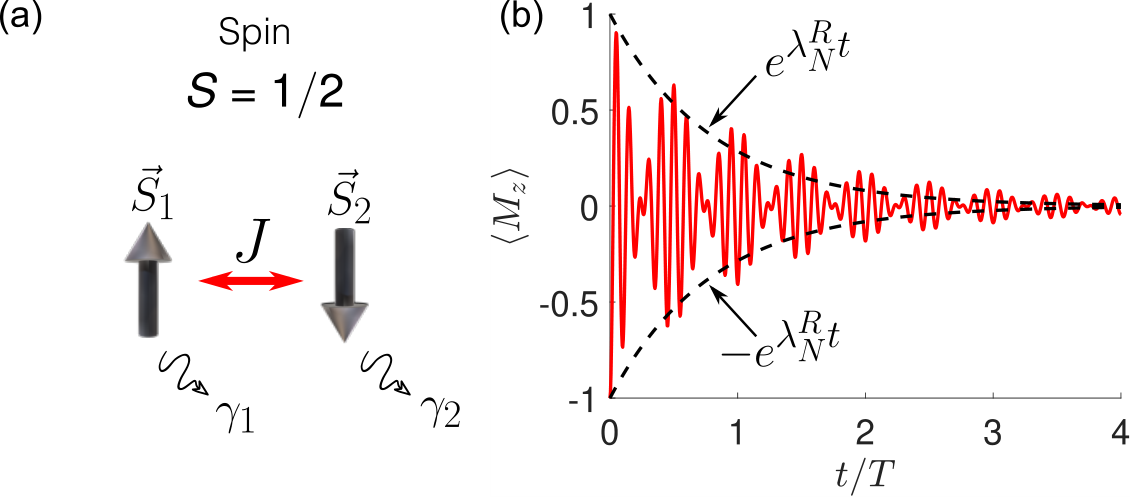
Figure 5: (a) Schematic representation of the dissipative Ising model. (b) Average magnetization along the zz direction for J=1J=1 and B=J/10B=J/10 and considering the initial condition ρ⁡(0)=|Ψ⁡(0)⟩​⟨Ψ⁡(0)|\rho(0)=|\Psi(0)\rangle\langle\Psi(0)|, with |Ψ⁡(0)⟩=|↓⟩1⊗|↓⟩2|\Psi(0)\rangle=\ket{\downarrow}_{1}\otimes\ket{\downarrow}_{2}. The time is divided by the natural period T=2​π/(2​B)T=2\pi/(2B). The envelope (dashed line) is calculated using the eigenvalue with the largest negative part λNR=−0.04\lambda_{N}^{R}=-0.04.

As the system consist in two interacting qubits, the density matrix ρ⁡(t)\rho(t) has a 4×44\times 4 size. As a consequence, ρ→​(t)\vec{\rho}(t) has exactly 1616 elements. This implies that we have 1616 eigenvalues associated with RkR_{k} and LkL_{k} matrices. However, the eigenvalues and eigenmatrices must be sorted with the same criteria. To do this, we introduce the function sortingEigenvalues()

1 function [R_sort,L_sort,lambda_sort] = sortingEigenvalues(dim,TOL,L)
2
3 [R,DR] = eig(L); % Right eigenvectors and eigenvalues
4 [L,DL] = eig(L'); % Left eigenvectors and eigenvalues
5 eig_R = diag(DR); % Right eigenvalues written as a vector
6 eig_L = diag(DL); % Left eigenvalues written as a vector
7 ind_RL = zeros(dim*dim,2);
8 count = 1;
9 for n=1:dim*dim % Sorting of eigenvalues
10 an = eig_R(n);
11 for m=1:dim*dim
12 bm = eig_L(m);
13 if(abs(real(an)-real(bm))<TOL && abs(imag(an)-imag(bm))<TOL && count<=dim*dim)
14 ind_RL(count,1) = n;
15 ind_RL(count,2) = m;
16 count = count + 1;
17 end
18 end
19 end
20 eig_L = eig_L(ind_RL(:,2)'); % Final sorting
21 eig_R = eig_R(ind_RL(:,1)');
22 L = L(:,ind_RL(:,2)');
23 R = R(:,ind_RL(:,1)');
24 lambda = eig_R;
25 [~,ind] = sort(lambda); % Sorting of eigenvalues
26 lambda_sort = lambda(ind); % \lambda_k eigenvalues
27 L = L(:,ind);
28 R = R(:,ind);
29
30 % Final R_sort and L_sort matrices
31 R_sort = cell(1,length(lambda_sort));
32 L_sort = cell(1,length(lambda_sort));
33 for k=1:length(lambda_sort)
34 R_sort{k} = reshape(R(:,k),dim,dim);
35 L_sort{k} = reshape(L(:,k),dim,dim);
36 Rk = R_sort{k};
37 Lk = L_sort{k};
38 Ck = trace(Lk*Rk);
39 Lk = Lk/sqrt(Ck); % Normalized left eigenmatrices
40 Rk = Rk/sqrt(Ck); % Normalized right eigenmatrices
41 R_sort{k} = Rk;
42 L_sort{k} = Lk;
43 end
44 end'

The above function returns the sorted eigenmatrices RkR_{k}, LkL_{k} and eigenvalues λk\lambda_{k} following a descending order for the real part of the eigenvalues: 0=λ1R≥λ2R≥…≥λN−1R≥λNR0=\lambda_{1}^{R}\geq\lambda_{2}^{R}\geq...\geq\lambda_{N-1}^{R}\geq\lambda_{N}^{R}, where the NN eigenvalues are decomposed as λk=λkR+i​λkI\lambda_{k}=\lambda^{R}_{k}+i\lambda_{k}^{I}. The first eigenvalue λ1=0\lambda_{1}=0 correspond to the steady state of the system, where L1=𝟙L_{1}=\mathds{1} [5, 24]. Also, the eigenvalues with k>1k>1 satisfy the condition λkR<0\lambda_{k}^{R}<0 leading to dissipation terms ∝eλkR​t\propto e^{\lambda_{k}^{R}t} in the general solution defined in equation (18). The eigenvalue with the largest negative real part (λNR\lambda_{N}^{R}) defines the envelope eλNR​te^{\lambda_{N}^{R}t} of the experimental observables (see figure 1-(b)). The normalized right (RkR_{k}) and left (LkL_{k}) eigenmatrices are calculated using the relations Rk = Rk/sqrt(Ck) and Lk = Lk/sqrt(Ck), where Ck = trace(Lk*Rk) is the normalization factor. Using the normalized matrices RkR_{k} and LkL_{k} we can compute any physical observable. By choosing the initial condition ρ⁡(0)=|Ψ⁡(0)⟩​⟨Ψ⁡(0)|\rho(0)=|\Psi(0)\rangle\langle\Psi(0)|, with |Ψ⁡(0)⟩=|↓⟩1⊗|↓⟩2|\Psi(0)\rangle=\ket{\downarrow}_{1}\otimes\ket{\downarrow}_{2}, we calculate the average magnetization ⟨Mz⟩=Tr​(Mz​ρ​(t))\langle M_{z}\rangle=\mbox{Tr}(M_{z}\rho(t)). The last part of the code read as

1 TOL = 1e-10;
2 [R_sort,L_sort,lambda_sort] = sortingEigenvalues(dim,TOL,L);
3
4 down = [0 1]'; % Quantum state down = [0 1]
5 Psi_0 = kron(down,down); % Initial wavefunction
6 rho_0 = Psi_0*Psi_0'; % Initial density matrix
7 Nt = 3000; % Number of steps for time
8 T = 2*pi/(2*B) ; % Period of time
9 ti = 0; % Intial time
10 tf = 4*T; % Final time
11 dt = (tf-ti)/(Nt-1); % Step for time
12 t = ti:dt:tf; % Time vector
13 Mz = zeros(size(t)); % Initial average magnetization
14 SSz = (kron(Sz,I)+kron(I,Sz))/2; % Operator S1^z+S2^z
15 for n=1:length(t) % Iteration to find general sulution of rho(t)
16 rho = zeros(dim,dim);
17 for k=1:length(lambda_sort)
18 Lk = L_sort{k};
19 Rk = R_sort{k};
20 ck = trace(rho_0*Lk);
21 rho = rho + ck*exp(lambda_sort(k)*t(n))*Rk; % General sulution for rho(t)
22 end
23 Mz(n) = trace(SSz*rho); % General sulution for Mz(t)
24 end
25 figure()
26 hold on
27 plot(t/T,real(Mz),'r-','LineWidth',3)
28 plot(t/T, exp(real(lambda_sort(end))*t),'k--','LineWidth',2)
29 plot(t/T,-exp(real(lambda_sort(end))*t),'k--','LineWidth',2)
30 hold off
31 xlabel('$Bt$','Interpreter','LaTex','Fontsize', 30)
32 ylabel('$\langle M_z \rangle$','Interpreter','LaTex','Fontsize', 30)
33 set(gca,'fontsize',21)

The numerical stability of the presented method crucially depends on the value of the step size d​tdt. The condition to have numerical stability is given by d​t≪1/maxk⁡(|λk|)dt\ll 1/\max_{k}(|\lambda_{k}|), where λk\lambda_{k} are the eigenvalues associated to the equation ℒ⁡(Rk)=λk​Rk\mathcal{L}(R_{k})=\lambda_{k}R_{k}. In the above example we have chosen d​t=0.0419dt=0.0419 since maxk⁡(|λk|)=2.2003\max_{k}(|\lambda_{k}|)=2.2003. For the rest of the examples we must ensure this condition.

In figure 5 we plotted the expected average magnetization ⟨Mz⟩\langle M_{z}\rangle for the dissipative two-spin system. In comparison with the non-dissipative case (see figure 1) the open Ising model shows a dissipative signal for ⟨Mz⟩\langle M_{z}\rangle. The envelope of this signal can be recognized as the exponential factor exp​(λNR​t)\mbox{exp}(\lambda_{N}^{R}t) with N=16N=16 in our case. This dissipative behaviour is a consequence of the losses introduced in the Markovian master equation.

3.2 Two-level system coupled to a photon reservoir

In this subsection, we applied the previous algorithm to a different system, say, a two-level system interacting with thermal photons. We consider the following Markovian master equation for the atom-field interaction [6]

d​ρd​t\displaystyle{d\rho\over dt} =\displaystyle= i​Ω2​[σ^++σ^−,ρ⁡(t)]+γ0​(Nph+1)​[σ^−​ρ​(t)​σ^−†−12​{σ^−†​σ^−,ρ⁡(t)}]\displaystyle{i\Omega\over 2}[\hat{\sigma}_{+}+\hat{\sigma}_{-},\rho(t)]+\gamma_{0}(N_{\rm ph}+1)\left[\hat{\sigma}_{-}\rho(t)\hat{\sigma}_{-}^{\dagger}-{1\over 2}\{\hat{\sigma}_{-}^{\dagger}\hat{\sigma}_{-},\rho(t)\}\right] (21)
+γ0​Nph​[σ^+​ρ​(t)​σ^+†−12​{σ^+†​σ^+,ρ⁡(t)}],\displaystyle+\gamma_{0}N_{\rm ph}\left[\hat{\sigma}_{+}\rho(t)\hat{\sigma}_{+}^{\dagger}-{1\over 2}\{\hat{\sigma}_{+}^{\dagger}\hat{\sigma}_{+},\rho(t)\}\right],

where Ω\Omega is the optical Rabi frequency, NphN_{\rm ph} is the mean number of photons at thermal equilibrium, and σ^+=|e⟩​⟨g|=σ−†\hat{\sigma}_{+}=|e\rangle\langle g|=\sigma_{-}^{\dagger}. To solve the open dynamics of the reduced two-level system we implement the following code:

1 Omega = 1; % Raby frequency from |1> to |2>
2 gamma0 = 0.2*Omega; % Decay rate
3 dim = 2; % Dimension Hilbert space two-level system
4 Is = eye(dim); % Identity matrix Hilbert space
5 v1 = Is(:,1); % Excited state for the atom
6 v2 = Is(:,2); % Ground state fro the atom
7 s11 = v1*v1'; % Atom operator sigma_{11}
8 s22 = v2*v2'; % Atom operator sigma_{22}
9 sp = v1*v2'; % Atom operator sigma_{+}
10 sm = v2*v1'; % Atom operator sigma_{-}
11 HL = -0.5*Omega*(sp+sm); % Hamiltonian of the two-level system
12 N = 0; % Mean number of photons at zero temperature
13 Lrad = gamma0*(N+1)*(kron(conj(sm),sm)-0.5*kron(Is,sm'*sm)-0.5*kron(sm.'*conj(sm),Is)) + ...
14 gamma0*N*(kron(conj(sp),sp)-0.5*kron(Is,sp'*sp)-0.5*kron(sp.'*conj(sp),Is));
15 L = -1i*kron(Is,HL)+1i*kron(HL.',Is)+Lrad; % Lindblad operator
16 TOL = 1e-6;
17 [R_sort,L_sort,lambda_sort] = sortingEigenvalues(dim,TOL,L);
18 psi_0 = v2; % Ground state
19 rho_0 = psi_0*psi_0'; % Initial density matrix
20 Nt = 100000; % Number of steps for time
21 ti = 0; % Initial time
22 tf = 50/Omega; % Final time
23 dt = (tf-ti)/(Nt-1); % Step time dt
24 t = ti:dt:tf; % Time vector
25 rho11 = zeros(size(t)); % Matrix elements \rho_{ij} = <i|\rho|j>
26 sigmap = zeros(size(t));
27 for n=1:Nt % General solution
28 rho = zeros(dim,dim);
29 for k=1:length(lambda_sort)
30 Lk = L_sort{k};
31 Rk = R_sort{k};
32 ck = trace(rho_0*Lk);
33 rho = rho + ck*exp(lambda_sort(k)*t(n))*Rk;
34 end
35 rho11(n) = rho(1,1);
36 sigmap(n) = trace(rho*sp);
37 end
38 % Exact Solution at zero temperature
39 % p_e: population excited state, sp = <\sigma_x>
40 mu = 1i*sqrt((gamma0/4)^2-Omega^2);
41 pe_exact = Omega^2/(gamma0^2+2*Omega^2)*(1-exp(-3*gamma0*t/4).*(cos(mu*t)+3*gamma0/4/mu*sin(mu*t)));
42 if gamma0~=0
43 sp_exact = -1i*Omega*gamma0/(gamma0^2+2*Omega^2)*(1-exp(-3*gamma0*t/4).*(cos(mu*t)+(gamma0/4/mu)-Omega^2/gamma0/mu*sin(mu*t)));
44 else
45 sp_exact = -1i/2*sin(Omega*t);
46 end
47 figure
48 box on
49 hold on
50 plot(t*Omega,real(rho11),'r-','Linewidth',2)
51 plot(t*Omega,pe_exact,'b--','Linewidth',2)
52 hold off
53 xlabel('$\Omega t$','Interpreter','LaTex','Fontsize', 30)
54 ylabel('$p_e(t)$','Interpreter','LaTex','Fontsize', 30)
55 legend({'$\mbox{Numerical}$','$\mbox{Exact}$'},'Interpreter','latex','Fontsize', 21,'Location','northeast')
56 set(gca,'fontsize',21)
57 xlim([0 50])
58
59 figure
60 box on
61 hold on
62 plot(t*Omega,imag(sigmap),'r-','Linewidth',2)
63 plot(t*Omega,imag(sp_exact),'b--','Linewidth',2)
64 hold off
65 xlabel('$\Omega t$','Interpreter','LaTex','Fontsize', 30)
66 ylabel('$\mbox{Im}\langle \hat{\sigma}_+ \rangle$','Interpreter','LaTex','Fontsize', 30)
67 legend({'$\mbox{Numerical}$','$\mbox{Exact}$'},'Interpreter','latex','Fontsize', 21,'Location','northeast')
68 set(gca,'fontsize',21)
69 xlim([0 50])

The numerical method used to solve the Markovian dynamics of the two-level system coupled to photons is based on the general solution presented in equation (18). After define the Lindblad operator in line 15 (see source code), we find the eigenmatrices and eigenvalues using the same function sortingEigenvalues() presented in the previous section. The value of the tolerance parameter TOL (line 16 of the code) is chosen in order to have a sufficient numerical precision to discriminate the real and imaginary parts of the most similar eigenvalues λk\lambda_{k}.

Figure 6: (a) Population of the excited state pe​(t)=⟨e|ρ⁡(t)|e⟩p_{e}(t)=\langle e|\rho(t)|e\rangle for a two-level system interacting with a photon reservoir at zero temperature. In both curves we use N=0N=0, γ0=0.2​Ω\gamma_{0}=0.2\Omega and Ω=1\Omega=1. (b) Imaginary part of the observable ⟨σ^+​(t)⟩\langle\hat{\sigma}_{+}(t)\rangle as a function of time. In both plots the red (solid) and blue (dashed) lines correspond to the numerical and exact calculations, respectively.

Following this procedure, in lines 30-33 of the source code, we calculated the density operator using the command rho = rho + ck*exp(lambda(k)*t(n))*Rk, where ck = trace(rho_0*Lk), lambda(k) are the eigenvalues, Rk are the right eigenmatrices, and rho_0 is the initial density matrix.

At zero temperature (Nph=0N_{\rm ph}=0) we have the following exact solutions

pe​(t)\displaystyle p_{e}(t) =\displaystyle= Ω2γ02+2​Ω2[1−e−3γ0t/4(cosμt+3​γ04​μsinμt)],\displaystyle{\Omega^{2}\over\gamma_{0}^{2}+2\Omega^{2}}\left[1-e^{-3\gamma_{0}t/4}\left(\cos\mu t+{3\gamma_{0}\over 4\mu}\sin\mu t\right)\right], (22)
⟨σ^+​(t)⟩\displaystyle\langle\hat{\sigma}_{+}(t)\rangle =\displaystyle= −i​Ω​γ0γ02+2​Ω2[1−e−3γ0t/4(cosμt+{γ04​μ−Ω2γ0​μ}sinμt)],\displaystyle{-i\Omega\gamma_{0}\over\gamma_{0}^{2}+2\Omega^{2}}\left[1-e^{-3\gamma_{0}t/4}\left(\cos\mu t+\left\{{\gamma_{0}\over 4\mu}-{\Omega^{2}\over\gamma_{0}\mu}\right\}\sin\mu t\right)\right], (23)

where μ=Ω2−(γ/4)2\mu=\sqrt{\Omega^{2}-(\gamma/4)^{2}}. In figure 6 we plotted the population pe​(t)=⟨e|ρ⁡(t)|e⟩p_{e}(t)=\langle e|\rho(t)|e\rangle and the imaginary part of ⟨σ^+⟩\langle\hat{\sigma}_{+}\rangle for Nph=0N_{\rm ph}=0. We observed a good agreement between the numerical and the exact solutions. Beyond the time evolution, the steady state of the system is a very useful information. For example, when the system reaches the steady state (t≫γ0−1t\gg\gamma_{0}^{-1}), the excited state and coherence can be found, ρe​ess=Ω2/(γ02+2​Ω2)\rho_{ee}^{\rm ss}=\Omega^{2}/(\gamma_{0}^{2}+2\Omega^{2}) and ρe​gss=i​Ω​γ0/(γ02+2​Ω2)\rho_{eg}^{\rm ss}=i\Omega\gamma_{0}/(\gamma_{0}^{2}+2\Omega^{2}). In our case, Ω=1\Omega=1 and γ0=0.2​Γ\gamma_{0}=0.2\Gamma resulting in ρe​ess=0.4902\rho_{ee}^{\rm ss}=0.4902 and ρe​gss=0.0980​i\rho_{eg}^{\rm ss}=0.0980i.

The numerical approach to obtain the density matrix in the steady state reads

ρssnum=c1​R1,\rho_{\rm ss}^{\rm num}=c_{1}R_{1}, (24)

This solution correspond to the particular case in which ρ˙=0\dot{\rho}=0. By looking our numerical simulations we obtain

ρssnum=(0.49020.0980​i−0.0980​i0.5098),\rho_{\rm ss}^{\rm num}=\left(\begin{array}[]{rr}0.4902&0.0980i\\ -0.0980i&0.5098\end{array}\right), (25)

Which exactly matches the theoretical predictions. Further extensions of this code to multiple level systems can be realized by changing the Hamiltonian and the dissipative contributions.

3.3 Time-local quantum master equation

In literature, the time-local quantum master equation in the secular approximation is presented as [7]

d​ρd​t=ℒNM​ρ​(t)=−i⁡[H^s,ρ⁡(t)]+∑i=1Ncγi​(t)​[L^i​ρ​(t)​L^i†−12​{L^i†​L^i,ρ⁡(t)}],{d\rho\over dt}=\mathcal{L}_{\rm NM}\rho(t)=-i[\hat{H}_{\rm s},\rho(t)]+\sum_{i=1}^{N_{\rm c}}\gamma_{i}(t)\left[\hat{L}_{i}\rho(t)\hat{L}_{i}^{\dagger}-{1\over 2}\{\hat{L}_{i}^{\dagger}\hat{L}_{i},\rho(t)\}\right], (26)

where γi​(t)\gamma_{i}(t) are the time-dependent rates associated with operators L^i\hat{L}_{i}. These rates can be obtained using a microscopic derivation ruled by the Hamiltonian describing the system-reservoir interaction [6]. In order to numerically solve this type of equations we adopt a different approach with respect to the Markovian case. To solve the non-Markovian dynamics we employed a predictor corrector integrator method [27, 16]. In the next section, we illustrate the main ideas by solving the pure-dephasing dynamics of the spin-boson model.

3.4 Pure-dephasing model and non-Markovianity

We consider the Hamiltonian for the pure dephasing spin-boson model (ℏ=1\hbar=1)

H=ωe​g2​σ^z+∑kωk​b^k†​b^k+σ^z2​∑k(gk​b^k+gk∗​b^k†),H={\omega_{eg}\over 2}\hat{\sigma}_{z}+\sum_{k}\omega_{k}\hat{b}_{k}^{\dagger}\hat{b}_{k}+\frac{\hat{\sigma}_{z}}{2}\sum_{k}\left(g_{k}\hat{b}_{k}+g_{k}^{\ast}\hat{b}^{\dagger}_{k}\right), (27)

where ωe​g\omega_{eg} is the bare frequency of the two-level system and ωk\omega_{k} are the boson frequencies. The exact time-local master equation in the interaction picture is [26]

d​ρd​t=γ⁡(t)2​[σ^z​ρs​(t)​σ^z†−{σ^z†​σ^z,ρ⁡(t)}]=γ⁡(t)2​[σ^z​ρs​(t)​σ^z−ρ⁡(t)].{d\rho\over dt}=\frac{\gamma(t)}{2}\left[\hat{\sigma}_{z}\rho_{s}(t)\hat{\sigma}_{z}^{\dagger}-\{\hat{\sigma}_{z}^{\dagger}\hat{\sigma}_{z},\rho(t)\}\right]=\frac{\gamma(t)}{2}\left[\hat{\sigma}_{z}\rho_{s}(t)\hat{\sigma}_{z}-\rho(t)\right]. (28)

The system-environment interaction is fully determined by the time-dependent dephasing rate (ℏ=1\hbar=1)

γ⁡(t)=∫0∞J⁡(ω)ω​coth⁡(ω2​kB​T)​sin⁡(ω​t)​𝑑ω,\gamma(t)=\int_{0}^{\infty}{J(\omega)\over\omega}\coth\left({\omega\over 2k_{B}T}\right)\sin(\omega t)\,d\omega, (29)

where J⁡(ω)=∑k|gk|2​δ​(ω−ωk)J(\omega)=\sum_{k}|g_{k}|^{2}\delta(\omega-\omega_{k}) is the spectral density function (SDF), kBk_{B} is the Boltzmann constant and TT is the reservoir temperature. We solve the dynamics for the following spectral density functions

J1​(ω)\displaystyle J_{1}(\omega) =\displaystyle= αωc1−sωse−ω/ωc,\displaystyle\alpha\omega_{\rm c}^{1-s}\omega^{s}e^{-\omega/\omega_{\rm c}}, (30)
J2​(ω)\displaystyle J_{2}(\omega) =\displaystyle= J0​ωs(ωω0+1)2​Γ/2(ω−ω0)2+(Γ/2)2,\displaystyle{J_{0}\omega^{s}\over\left({\omega\over\omega_{0}}+1\right)^{2}}\frac{\Gamma/2}{(\omega-\omega_{0})^{2}+(\Gamma/2)^{2}}, (31)

where J1​(ω)J_{1}(\omega) was originally introduced in the context of dissipative two-level systems [28]. Physically, α\alpha is the system-environment coupling strength, s≥0s\geq 0 is a parameter, and ωc\omega_{c} is the cut-off frequency. Usually, three cases are defined: i) 0<s<10<s<1 (sub-Ohmic), s=1s=1 (Ohmic), and s>1s>1 (super-Ohmic). The spectral density function J2​(ω)J_{2}(\omega) comes from the dynamics of quantum dots [29] but also can describe localized-phonons in color centers in diamond [Ariel2019]. In order to quantify the degree of non-Markovianity (NM) we use the following measure [30, 31]

𝒩γ​(t)=12​∫0t(|γc​(τ)|−γc​(τ))​𝑑τ,\mathcal{N}_{\gamma}(t)={1\over 2}\int_{0}^{t}(|\gamma^{\rm c}(\tau)|-\gamma^{\rm c}(\tau))\,d\tau, (32)

where γc​(t)\gamma^{\rm c}(t) is the canonical rate when the master equation is written in the form ρ˙=γc​(t)​[L^z​ρs​(t)​L^z†−(1/2)​{L^z†​L^z,ρ⁡(t)}]\dot{\rho}=\gamma^{\rm c}(t)\left[\hat{L}_{z}\rho_{s}(t)\hat{L}_{z}^{\dagger}-(1/2)\{\hat{L}_{z}^{\dagger}\hat{L}_{z},\rho(t)\}\right] with Tr​(Lz†​Lz)=1\mbox{Tr}(L_{z}^{\dagger}L_{z})=1 [33]. From equation (28) we recognize Lz=σz/2L_{z}=\sigma_{z}/\sqrt{2} and therefore we have γc​(t)=γ​(t)\gamma^{\rm c}(t)=\gamma(t). In what follows, we implement a code to numerically solve the time-dependent rate, the coherence, and the NM measure introduced in equation (32).

1 sz = [1 0; % Pauli matrix s_z
2 0 -1];
3 Nw = 5000; % Number of points for \omega
4 wi = 0.01; % Initial frequency
5 wf = 5; % Final frequency
6 dw = (wf-wi)/(Nw-1); % Step frequency d\omega
7 w = wi:dw:wf; % Frequency vector
8 alpha = 5; % Strength spectral density function J1(w)
9 s = 2.5; % Ohmic-parameter s
10 wc = 0.1; % Cut-off frequency
11 J1 = alpha*wc^(1-s)*w.^s.*exp(-w/wc); % Spectral density funcion J1(w)
12 J0 = 0.2; % Strength spectral density function J2(w)
13 w0 = 2; % Resonant frequency
14 Gamma = 0.1; % Width of the spectral density function J2(w)
15 J2 = J0*(Gamma/2)./((w-w0).^2+(Gamma/2)^2).*w.^s./(w/w0+1).^2; % Spectral density funcion J2(w)
16 figure
17 box on
18 hold on
19 plot(w,J1,'r-','Linewidth',2)
20 plot(w,J2,'b-','Linewidth',2)
21 hold off
22 xlabel('$\omega$','Interpreter','LaTex','Fontsize', 30)
23 ylabel('$J(\omega)$','Interpreter','LaTex','Fontsize', 30)
24 legend({'$J_1(\omega)$','$J_2(\omega)$'},'Interpreter','latex','Fontsize', 21,'Location','northeast')
25 set(gca,'fontsize',21)
26 xlim([0 5])
27 Nt = 5000; % Number of points for time
28 ti = 0; % Initial time
29 tf = 100; % Final time
30 dt = (tf-ti)/(Nt-1); % Step time dt
31 t = ti:dt:tf; t= t'; % Time vector
32 Psi_0 = [1 1]'/sqrt(2); % Initial wavefunction
33 rho1 = Psi_0*Psi_0'; % Initial density matrix
34 rho2 = rho1;
35 p11 = zeros(size(t));
36 p22 = zeros(size(t));
37 p12 = zeros(size(t));
38 p21 = zeros(size(t));
39 wa = ones(size(t))*w; % Auxiliar frecuency vector
40 J1a = ones(size(t))*J1; % Auxiliar J1 vector
41 J2a = ones(size(t))*J2; % Auxiliar J2 vector
42 ta = t*ones(size(w)); % Auxiliar time vector
43 T = 0.001*w0; % Temperature
44 gamma1 = sum(J1a./wa.*sin(wa.*ta).*coth(wa/T/2),2)*dw; % Rate gamma_1(t)
45 gamma_1_teo = alpha*wc*gamma(s)*sin(s*atan(wc*t))./(1+(wc*t).^2).^(s/2);
46 gamma2 = sum(J2a./wa.*sin(wa.*ta).*coth(wa/T/2),2)*dw; % Rate gamma_2(t)
47 figure()
48 box on
49 hold on
50 plot(t,gamma1,'r-','Linewidth',2)
51 plot(t,gamma_1_teo,'k--','Linewidth',2)
52 plot(t,gamma2,'b-','Linewidth',2)
53 hold off
54 xlabel('$t$','Interpreter','LaTex','Fontsize', 30)
55 ylabel('$\gamma(t)$','Interpreter','LaTex','Fontsize', 30)
56 legend({'$\gamma_1(t)$','$\gamma_1^{\rm teo}(t)$','$\gamma_2(t)$'},'Interpreter','latex','Fontsize', 21,'Location','northeast')
57 set(gca,'fontsize',21)
58 xlim([0 100])
59 nk = 15; % nk steps per interval dt
60 C1 = zeros(size(t));
61 C2 = zeros(size(t));
62 N1 = zeros(size(t));
63 N2 = zeros(size(t));
64 for n = 1:length(t)
65 for k = 1:nk
66 L1 = gamma1(n)*(sz*rho1*sz -rho1); % Lindbladian for gamma_1
67 L2 = gamma2(n)*(sz*rho2*sz -rho2); % Lindbladian for gamma_2
68 rho1_pred = rho1 + L1*dt/nk; % Predictor \rho_1
69 rho2_pred = rho2 + L2*dt/nk; % Predictor \rho_2
70 rho1_m = 0.5*(rho1+rho1_pred); % Mean \rho_1
71 rho2_m = 0.5*(rho1+rho2_pred); % Mean \rho_1
72 L1 = gamma1(n)*(sz*rho1_m*sz -rho1_m); % Lindbladian using mean \rho_1
73 L2 = gamma2(n)*(sz*rho2_m*sz -rho2_m); % Lindbladian using mean \rho_2
74 rho1 = rho1 + L1*dt/nk; % Density matrix \rho_1
75 rho2 = rho2 + L2*dt/nk; % Density matrix \rho_2
76 end
77 C1(n) = 2*abs(rho1(1,2)); % Coherence C1(t)
78 C2(n) = 2*abs(rho2(1,2)); % Coherence C2(t)
79 f1 = (abs(gamma1(1:n))-gamma1(1:n));
80 N1(n) = sum(f1)*dt; % Degree of non-Markovianity for gamma_1
81 f2 = (abs(gamma2(1:n))-gamma2(1:n));
82 N2(n) = sum(f2)*dt; % Degree of non-Markovianity for gamma_2
83 end
84 figure()
85 box on
86 hold on
87 plot(t,C1,'r-','Linewidth',2)
88 plot(t,C2,'b-','Linewidth',2)
89 hold off
90 xlabel('$t$','Interpreter','LaTex','Fontsize', 30)
91 ylabel('$C(t)$','Interpreter','LaTex','Fontsize', 30)
92 legend({'$C_1(t)$','$C_2(\omega)$'},'Interpreter','latex','Fontsize', 21,'Location','northeast')
93 set(gca,'fontsize',21)
94 xlim([0 50])
95
96 figure()
97 box on
98 hold on
99 plot(t,N1,'r-','Linewidth',2)
100 plot(t,N2,'b-','Linewidth',2)
101 hold off
102 xlabel('$t$','Interpreter','LaTex','Fontsize', 30)
103 ylabel('$\mathcal{N}_{\gamma}(t)$','Interpreter','LaTex','Fontsize', 30)
104 legend({'$\mathcal{N}_{\gamma_1}(t)$','$\mathcal{N}_{\gamma_2}(t)$'},'Interpreter','latex','Fontsize', 21,'Location','best')
105 set(gca,'fontsize',21)
106 xlim([0 100])'

Figure 7: (a) Spectral density functions J1​(ω)J_{1}(\omega) and J2​(ω)J_{2}(\omega). For the spectral density functions we set the values α=0.5\alpha=0.5, s=2.5s=2.5, ωc=0.1\omega_{\rm c}=0.1, J0=0.2J_{0}=0.2, ω0=2\omega_{0}=2, and Γ=0.1\Gamma=0.1. (b) Time-dependent rates γ1​(t)\gamma_{1}(t) and γ2​(t)\gamma_{2}(t) associated with J1​(ω)J_{1}(\omega) and J2​(ω)J_{2}(\omega), respectively. The rates are calculated at T=10−3​ω0T=10^{-3}\omega_{0} (low-temperature). (c) Coherence function C1​(t)C_{1}(t) and C2​(t)C_{2}(t) associated with γ1​(t)\gamma_{1}(t) and γ2​(t)\gamma_{2}(t), respectively. (d) Degree of non-Markovianity 𝒩γ​(t)=(1/2)​∫0t(|γ⁡(τ)|−γ⁡(τ))​𝑑τ\mathcal{N}_{\gamma}(t)=(1/2)\int_{0}^{t}(|\gamma(\tau)|-\gamma(\tau))\,d\tau.

In figure 7-(a) we plotted the spectral density functions J1​(ω)J_{1}(\omega) (red) and J2​(ω)J_{2}(\omega) (blue) given in equation (30) and (31) for s=2.5s=2.5 and ωc=0.1\omega_{\rm c}=0.1. The super-Ohmic function J1​(ω)J_{1}(\omega) reaches a maximum around ω≈0.25\omega\approx 0.25 and quickly decreases due to the cut-off frequency term exp(−ω/ωc)\mbox{exp}(-\omega/\omega_{\rm c}). On the contrary, the spectral density function J2​(ω)J_{2}(\omega) is strongly localized at the frequency ω0=2\omega_{0}=2 with a full with at half maximum equal to Γ=0.1\Gamma=0.1. The associated rates γ1​(t)\gamma_{1}(t) and γ2​(t)\gamma_{2}(t) are illustrated in figure 7-(b). These time-dependent rates are calculated at low temperature T=10−3​ω0T=10^{-3}\omega_{0}. The damped oscillations of γ2​(t)\gamma_{2}(t) are a consequence of the strong interaction with the localized mode ω0\omega_{0}. In fact, the periods of the signal are approximately given by T≈2​π/ω0≈3.14T\approx 2\pi/\omega_{0}\approx 3.14. On the other hand, the rate γ1​(t)\gamma_{1}(t) is positive in the time region 0≤t≤30.80\leq t\leq 30.8, while for t>30.8t>30.8 the curve asymptotically reaches a constant negative value. In the low-temperature regime one theoretically obtains γ1teo​(t)=α​ωc​Γ​(s)​sin⁡[s​tan−1⁡(ωc​t)]/[1+(ωc​t)2]s/2\gamma_{1}^{\rm teo}(t)=\alpha\omega_{\rm c}\Gamma(s)\sin[s\tan^{-1}(\omega_{\rm c}t)]/[1+(\omega_{\rm c}t)^{2}]^{s/2} [32] with Γ⁡(s)\Gamma(s) being the gamma function (see dashed curve in figure 7-(a)). Thus, the negative region of γ1​(t)\gamma_{1}(t) is stablished by the condition 3​tan−1⁡(ωc​t)>π3\tan^{-1}(\omega_{\rm c}t)>\pi leading to the critical time tcrit=tan⁡(π/s)/ωc≈30.8t_{\rm crit}=\tan(\pi/s)/\omega_{\rm c}\approx 30.8, in good agreement with the numerical calculations.

The coherence functions C⁡(t)=∑i≠j|ρi​j​(t)|=2​|ρe​g​(t)|C(t)=\sum_{i\neq j}|\rho_{ij}(t)|=2|\rho_{eg}(t)| [34] are shown in figure 7-(c) for the initial condition ρ⁡(0)=|Ψ⁡(0)⟩​⟨Ψ⁡(0)|\rho(0)=|\Psi(0)\rangle\langle\Psi(0)| with Ψ(0)⟩=(|e⟩+|g⟩)/2\Psi(0)\rangle=(|e\rangle+|g\rangle)/\sqrt{2}. The super-Ohmic spectral density function J1​(ω)J_{1}(\omega) induces a monotonic decreasing behaviour in the coherence while the localized model introduces oscillations. These oscillations can be understood as a back-flow of quantum information between the system and the environment. Finally, the degree of NM 𝒩γ​(t)\mathcal{N}_{\gamma}(t) is calculated and shown in figure 7-(d). As expected, the localized model evidences a high degree of NM at any time in comparison with the super-Ohmic model. This can be explained in terms of the fast oscillations observed in the rate γ2​(t)\gamma_{2}(t) and the coherence C2​(t)C_{2}(t). Further extensions of this code can be easily done by assuming different terms in the Lindbladian and modifying the model for the environment.

4 Concluding remarks

In summary, we have developed selected examples to show how to code many-body dynamics in relevant quantum systems using the high-level matrix calculations in MATLAB. We oriented our discussion and examples to the fields of quantum optics and condensed matter, and we expect that the codes shown here will be valuable for graduate students and researchers that begin in these fields. Moreover, the simplicity of the codes will allow the reader to extend it to other similar problems. We consider that these codes can be used as a starting toolbox for research projects involving closed and open quantum systems.

5 Acknowledgments

The authors would like to thank Fernando Crespo for the valuable codes in Python for comparison. AN acknowledges financial support from Universidad Mayor through the Postdoctoral fellowship. RC and DT acknowledge financial support from Fondecyt Iniciación No. 11180143.

References

References

  • [1] Jaynes E T and Cummings F W 1963 Comparison of Quantum and Semiclassical Radiation Theories with Applications to the Beam Maser Proc. IEEE. 51 89.
  • [2] Schmidt S and Blatter G 2009 Strong Coupling Theory for the Jaynes-Cummings-Hubbard Model, Phys. Rev. Lett. 103 086403.
  • [3] Porras D and Cirac J I 2004 Effective Quantum Spin Systems with Trapped Ions Phys. Rev. Lett. 92 207901.
  • [4] Aspelmeyer M, Kippenberg T J, and Marquardt F 2014 Cavity optomechanics Rev. Mod. Phys. 86 1391.
  • [5] Rose D C, Macieszczak K, Lesanovsky I, and Garrahan J P 2016 Metastability in an open quantum Ising model Phys. Rev. E 94 052132.
  • [6] Breuer H and Petruccione F 2002 The Theory of Open Quantum Systems (Oxford University Press, Oxford).
  • [7] Vega I and Alonso D 2017 Dynamics of non-Markovian open quantum systems Rev. Mod. Phys. 89, 015001.
  • [8] Filippov S N and Chruściński D, 2018 Time deformations of master equations Phys. Rev. A 98 022123.
  • [9] Norambuena A, Maze J R, Rabl P, and Coto R 2020 Quantifying phonon-induced non-Markovianity in color centers Phys. Rev. A 101 022110.
  • [10] Schmidt B and Lorenz U 2017 WavePacket: A Matlab package for numerical quantum dynamics. I: Closed quantum systems and discrete variable representations Computer Physics Communications 213 223.
  • [11] Schmidt B and Hartmann C 2018 WavePacket: A Matlab package for numerical quantum dynamics. II: Open quantum systems, optimal control, and model reduction Computer Physics Communications 228 229.
  • [12] Schmidt B, Klein R and Araujo L C 2019 WavePacket: A Matlab package for numerical quantum dynamics. III: Quantum-classical simulations and surface hopping trajectories J. Comput. Chem. 40 2677.
  • [13] Cooper I, Doing Physics with Matlab: Quantum Mechanics, Schrodinger Equation, Time independent bound states, http://www.physics.usyd.edu.au/teach_res/mp/quantum/doc/schrodinger.pdf.
  • [14] Chelikowsky R, Introductory Quantum Mechanics with MATLAB: For atoms, Molecules, Clusters and Nanocrystals, Wiley-VCH, Weinheim, Germany, 2019.
  • [15] Tan S M, Quantum Optics Toolbox for MATLAB, https://github.com/jevonlongdell/qotoolbox.
  • [16] Korsch H J and Rapedius K 2016 Computations in Quantum Mechanics Made Easy Europ. J. Phys. 37 055410.
  • [17] Shcrödinger E 1926 An Undulatory Theory of the Mechanics of Atoms and Molecules Phys. Rev. 28 1049.
  • [18] Zunkovic B, Heyl M, Knap M and Silva A 2016 Dynamical Quantum Phase Transitions in Spin Chains with Long-Range Interactions: Merging different concepts of non-equilibrium criticality Phys. Rev. Lett. 120 130601.
  • [19] Halimeh J C and Zauner-Stauber V 2017 Dynamical phase diagram of spin chains with long-range interactions Phys. Rev. B 96 134427.
  • [20] Jurcevic P, Shen H, Hauke P, Maier C, Brydges T, Hempel C, Lanyon B P, Heyl M, Blatt R and Roos F 2017 Direct Observation of Dynamical Quantum Phase Transitions in an Interacting Many-Body System Phys. Rev. Lett. 119 080501.
  • [21] Moler C and Van Loan C 2003 Nineteen Dubious Ways to Compute the Exponential of a Matrix, Twenty-Five Years Later SIAM Rev. 45 3–49.
  • [22] Figueroa J, Rogan J, Valdivia J A, Kiwi M, Romero G and Torres F 2018 Nucleation of superfluid-light domains in a quenched dynamics Scientific Reports 8 15603.
  • [23] Wang Q and Bernal F P 2019 Excited-state quantum phase transition and the quantum-speed-limit time Phys. Rev. A 100 022118.
  • [24] Macieszczak K, Guţă M, Lesanovsky I and Garrahan J P 2016 Towards a Theory of Metastability in Open Quantum Dynamics Phys. Rev. Lett. 116 240404.
  • [25] Navarrete-Benlloch C 2015 Open systems dynamics: Simulating master equations in the computer arXiv:1504.05266.
  • [26] Luczka J 1990 Spin in Contact With Thermostat: Exact Rreduced Dynamics Physica A 167 919.
  • [27] Press W H, Teukolsky S A, Vetterling W T and Flannery B P 2007 Numerical Recipes (Cambridge University Press, London, 3. edition).
  • [28] Leggett A J, Chakravarty S, Dorsey A T, Fisher M P, Garg A and Zwerger W 1987 Dynamics of the dissipative two-state system Rev. Mod. Phys. 59 1.
  • [29] Wilson-Rae I and Imamoğlu A 2002 Quantum dot cavity-QED in the presence of strong electron-phonon interactions Phys. Rev. B 65 235311.
  • [30] Rivas A, Huelga S F and Plenio M B 2010 Entanglement and Non-Markovianity of Quantum Evolutions Phys. Rev. Lett. 105 050403.
  • [31] Rivas A, Huelga S F and Plenio M B 2014 Quantum non-Markovianity: Characterization, Quantification and Detection Rep. Prog. Phys. 77 094001.
  • [32] Haikka P, Johnson T H and Maniscalco 2013 S Non-Markovianity of local dephasing channels and time-invariant discord Phys. Rev. A 87 010103(R).
  • [33] Hall M J, Cresser J D, Li L and Andersson E 2014 Canonical form of master equations and characterization of non-Markovianity Phys. Rev. A 89 042120.
  • [34] Baumgratz T, Cramer M and Plenio M B 2014 Quantifying Coherence Phys. Rev. Lett. 113 140401.