A Homotopy Method Based on Theory of Functional ConnectionsJournal: J COMPUT APPL MATH

Consider the zero-finding problem

where $\boldsymbol{x}\in\mathbb{R}^{n}$ and $\boldsymbol{F}:\mathbb{R}^{n}\to\mathbb{R}^{n}$ is a $\mathcal{C}^{2}$ function. Newton’s method is widely used to solve problem (1). However, it fails if the initial guess solution lies beyond its convergence domain, or singular points are encountered during iterations. These issues are likely in high-sensitive, nonlinear systems.

Homotopy is an effective strategy to solve difficult zero-finding problems, which lacks a priori knowledge on good initial guesses Allgower and Georg 2003. To solve Eq. (1), one may define a homotopy or deformation function ${\boldsymbol{\Gamma}}({\kappa,\boldsymbol{x}}):\mathbb{R}\times\mathbb{R}^{n}\to\mathbb{R}^{n}$ such that

where $\kappa\in[0,1]$ is the homotopy parameter and $\boldsymbol{G}(\boldsymbol{x}):\mathbb{R}^{n}\to\mathbb{R}^{n}$ is a user-defined, auxiliary function. Typically, solving $\boldsymbol{G}(\boldsymbol{x})=\boldsymbol{0}$ is easier than solving Eq. (1). The convex homotopy function is the commonly used form for $\boldsymbol{\Gamma}$:

Three types of homotopy are commonly used Rahimian et al. 2011, depending on $\boldsymbol{G}$:

1. 1.

   Newton homotopy, $\boldsymbol{G}(\boldsymbol{x})\coloneqq\boldsymbol{F}(\boldsymbol{x})-\boldsymbol{F}(\boldsymbol{x}_{0})$

2. 2.

   Fixed-point homotopy, $\boldsymbol{G}(\boldsymbol{x})\coloneqq\boldsymbol{x}-\boldsymbol{x}_{0}$

3. 3.

   Affine homotopy, $\boldsymbol{G}(\boldsymbol{x})\coloneqq A\left(\boldsymbol{x}-\boldsymbol{x}_{0}\right)$

where $\boldsymbol{x}_{0}$ is the solution to $\boldsymbol{G}(\boldsymbol{x})=\boldsymbol{0}$ and $A$ is a $n\times n$ matrix.

Under regularity assumptions Allgower and Georg 2003, Bhaya and Pazos 2013, defining the homotopy function inherently generates a unique curve $\boldsymbol{c}(\theta)\coloneqq\boldsymbol{\Gamma}^{-1}(\boldsymbol{0}):J\to\mathbb{R}^{n}$ for some open interval $J\subset\mathbb{R}$ starting from the initial solution $\boldsymbol{x}_{0}$, which contains points satisfying the consistency condition $\boldsymbol{\Gamma}(\kappa,\boldsymbol{x})=\boldsymbol{0}$. The tracked solution curve in $\mathbb{R}^{n+1}$ is called homotopy path or zero curve. With reference to Fig. 1, the homotopy paths can be mainly classified in five Types Watson 2002:

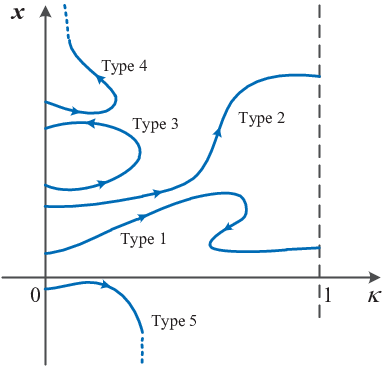
1. 1)

   The homotopy path ends in $\{1\}\times\mathbb{R}^{n}$, with non-monotonic $\kappa$;

2. 2)

   The homotopy path ends in $\{1\}\times\mathbb{R}^{n}$, with monotonic $\kappa$;

3. 3)

   The homotopy path returns to a solution of $\boldsymbol{\Gamma}(0,\boldsymbol{x})$ in $\{0\}\times\mathbb{R}^{n}$;

4. 4)

   The homotopy path is unbounded, with non-monotonic $\kappa\in[0,1)$;

5. 5)

   The homotopy path is unbounded, with monotonic $\kappa\in[0,1)$.

Homotopy methods attempt to track the homotopy path starting from $(0,\boldsymbol{x}^{*}(0))$ to $(1,\boldsymbol{x}^{*}(1))$. When this happens, one zero of Eq. (1) is found. The sufficient conditions for the existence of the homotopy path are given by probability-one homotopy theory Watson 2002, Chow et al. 1978, based on differential geometry concepts.

The parametrized Sard’s theorem indicates that for almost all $\boldsymbol{a}\in U$, the zero set of $\boldsymbol{\rho}_{a}$ consists of smooth, nonintersecting curves Watson 2002. In the following, we take $U\equiv\mathbb{R}^{n}$ and $V\equiv\mathbb{R}^{p}$.

Transversality is hard to verify for arbitrary $\boldsymbol{a}\in\mathbb{R}^{p}$, and a proper $\boldsymbol{a}$ is required to construct the homotopy function. For example, fixed-point homotopy methods require selecting a proper $\boldsymbol{x}_{0}$. However, in current homotopy methods Allgower and Georg 2003, $\boldsymbol{a}$ is manually selected and it cannot vary during iterations. Thus, the success of the entire procedure relies heavily on the initial point chosen, and thus once again on the empirical knowledge of the problem.

Once the homotopy function is defined, the focus is on tracking its implicitly defined path. Two predictor-corrector methods are reviewed: discrete continuation method (DCM) and pseudo-arclength method (PAM).

The Theory of Functional Connections (TFC) is the extension of the Theory of Connections (TOC) Mortari 2017a. The latter investigates the arbitrary connections between points by constructing a constrained function expressed in terms of an auxiliary function Mortari 2017a, Mortari 2018. It has the property that no matter what the auxiliary function is, the constrained function always satisfies a prescribed set of constraints.

Suppose we define the scalar function

where $y(\eta)$ and $g(\eta)$ are the constrained function and auxiliary function, respectively, whereas $\eta\in\left[\eta_{0},\eta_{f}\right]$ is the independent variable. It is easy to verify that Eq. (5) inherently satisfies $y(\eta_{0})=y_{0}$ and $y(\eta_{f})=y_{f}$ regardless of the specific choice of $g(\eta)$ (note that $g_{0}=g(\eta_{0})$ and $g_{f}=g(\eta_{f})$). Therefore, the line $y(\eta)$ will always connect the points $P_{0}=(\eta_{0},y_{0})$ and $P_{f}=(\eta_{f},y_{f})$. Eq. (5) is the generalization of interpolation formulae: it is not the interpolating expression for a class of functions but for all functions Mortari 2017a.

In the multi-dimensional case, the two-point condition is

where $\boldsymbol{y}\in\mathbb{R}^{n}$. The general expression of the constrained function $\boldsymbol{y}(\eta)$ is

where $P_{1,2}:\mathbb{R}\to\mathbb{R}^{n\times n}$ are matrices whose elements are scalar-valued functions of $\eta$, while $\boldsymbol{c}_{1,2}\in\mathbb{R}^{n}$ are constant vectors of weights Mortari 2017a. Substituting Eq. (6) into Eq. (7) and solving for $\boldsymbol{c}_{1,2}$ yields

where again $\boldsymbol{g}_{0}=\boldsymbol{g}(\eta_{0})$ and $\boldsymbol{g}_{f}=\boldsymbol{g}(\eta_{f})$. Moreover

The selection of $P_{1,2}(\eta)$ in Eq. (7) must ensure the existence of $Q_{ij}$ in Eq. (9). Substituting Eqs. (8) and (9) into Eq. (7) gives the general form of constrained function

The constrained function $\boldsymbol{y}(\eta)$ in Eq. (10) defines arbitrary connection paths between $\boldsymbol{y}_{0}$ and $\boldsymbol{y}_{f}$ produced by the infinitely possible choices of $\boldsymbol{g}(\eta)$. The constrained function for arbitrary boundary conditions can also be established Mortari 2017a. The Theory of Functional Connections (TFC) extends the idea above to construct the constrained function on a functional domain Mortari 2018.

From a geometrical point of view, the homotopy function defines the solution curve connecting the two zero-finding problems defined at the boundaries of $\kappa$, which satisfy Eq. (2). Analogously, the constrained function in the TFC connects points at the boundaries of $\eta$. Interpreting the constrained function as describing an homotopy path is therefore natural.

In Eq. (10), replacing the constrained function $\boldsymbol{y}(\eta)$ by the homotopy function $\boldsymbol{\Gamma}(\eta,\boldsymbol{x})$, and $\boldsymbol{y}_{0}$, $\boldsymbol{y}_{f}$ by $\boldsymbol{G}(\boldsymbol{x})$, $\boldsymbol{F}(\boldsymbol{x})$, respectively, we have

The auxiliary function $\boldsymbol{g}(\eta)$ can be expressed as a linear combination of basis functions with corresponding weights, that is

where $\boldsymbol{h}(\eta):\mathbb{R}\to\mathbb{R}^{m}$ is the vector of basis functions, whereas $\Omega\in\mathbb{R}^{n\times m}$ is the matrix of weights. Note that $\boldsymbol{g}_{0}=\Omega\boldsymbol{h}_{0}$ and $\boldsymbol{g}_{f}=\Omega\boldsymbol{h}_{f}$, where $\boldsymbol{h}_{0}=\boldsymbol{h}(\eta_{0})$ and $\boldsymbol{h}_{f}=\boldsymbol{h}(\eta_{f})$. A linear map between $\kappa\in\left[0,1\right]$ and $\eta\in[\eta_{0},\eta_{f}]$ is also used:

Substituting Eqs. (12) and (13) into Eq. (11) yields

Notice that $\boldsymbol{\Gamma}$ in Eq. (14), beside the natural dependence on $\kappa$ and $\boldsymbol{x}$, is also a function of the free parameter $\Omega$, which can be varied to steer the solution curve from $\boldsymbol{G}^{-1}(\boldsymbol{0})$ to $\boldsymbol{F}^{-1}(\boldsymbol{0})$.

It is convenient to isolate in Eq. (14) the part depending on $\kappa$ and $\boldsymbol{x}$ only

where

By taking the partial derivative of Eq. (15) w.r.t. $\boldsymbol{x}$, we find that

indicating that when a limit point is encountered both Jacobian matrices are singular, regardless of the selection of $\Omega$. In order to regularize $\partial\boldsymbol{\Gamma}/\partial\boldsymbol{x}$ by varying $\Omega$, we let the basis functions $\boldsymbol{h}$ to depend on the present solution $\boldsymbol{x}$ as well; that is, $\boldsymbol{h}=\boldsymbol{h}(\kappa,\boldsymbol{x})$. Thus, Eq. (15) becomes

where

Inspired by Eq. (17), the formal definition of TFC-based homotopy is given.

In traditional homotopy methods (e.g., Newton homotopy), the term $\boldsymbol{a}$ in the homotopy function $\boldsymbol{\rho}_{a}(\kappa,\boldsymbol{x})$ in Theorem 1 is set at the beginning of the continuation procedure (e.g., by providing the solution $\boldsymbol{x}(0)$ to the initial problem $\boldsymbol{G}(\boldsymbol{x})=\boldsymbol{0}$) and so is the homotopy path. The TFC-based homotopy function $\hat{\boldsymbol{\rho}}_{a}(\kappa,\boldsymbol{x},\boldsymbol{\varepsilon})$ is the generalization of $\boldsymbol{\rho}_{a}(\kappa,\boldsymbol{x})$. Here, although $\boldsymbol{a}$ is fixed, $\boldsymbol{\epsilon}$ brings in flexibility in the homotopy path while not affecting the boundary conditions, Eq. (2). The TFC-based homotopy function implicitly defines infinite homotopy paths because of the infinite possible selections of $\boldsymbol{\epsilon}$. Moreover, condition ii) in Definition 2 enables regularizing the path by varying $\boldsymbol{\epsilon}$. Therefore, it is a tool to recover improperly defined paths, by detecting them and switching to different, yet feasible, homotopy paths.

Equation (17) provides a general form of TFC-based homotopy function. Here, $\boldsymbol{\Gamma}_{0}(\kappa,\boldsymbol{x})$ is equivalent to $\boldsymbol{\rho}_{a}(\kappa,\boldsymbol{x})$ and $\Omega$ can be seen as $\boldsymbol{\epsilon}$ (see Appendix). Let $\tau=e^{\eta_{0}-\eta_{f}}$, the following three examples are given based on different choice of $P_{1,2}(\eta)$

1. 1.

   For $P_{1}=I$ and $P_{2}={\eta}I$

   $$\boldsymbol{\Gamma}(\kappa,\boldsymbol{x},\Omega)=\Omega\left(\boldsymbol{h}(\kappa,\boldsymbol{x})+(\kappa-1)\boldsymbol{h}_{0}(\boldsymbol{x})-\kappa\boldsymbol{h}_{f}(\boldsymbol{x})\right)+\boldsymbol{\Gamma}_{0}(\kappa,\boldsymbol{x})$$

   (19)

2. 2.

   For $P_{1}=I$ and $P_{2}=e^{\eta}I$

   $\displaystyle\boldsymbol{\Gamma}(\kappa,\boldsymbol{x},\Omega)=\Omega\left(\boldsymbol{h}(\kappa,\boldsymbol{x})-\dfrac{1-\tau^{(1-\kappa)}}{1-\tau}\boldsymbol{h}_{0}(\boldsymbol{x})-\dfrac{-\tau+\tau^{(1-\kappa)}}{1-\tau}\boldsymbol{h}_{f}(\boldsymbol{x})\right)+\boldsymbol{\Gamma}_{0}(\kappa,\boldsymbol{x})$

   (20)

3. 3.

   For $P_{1}=I$ and $P_{2}=e^{-\eta}I$

   $$\boldsymbol{\Gamma}(\kappa,\boldsymbol{x},\Omega)=\Omega\left(\boldsymbol{h}(\kappa,\boldsymbol{x})-\dfrac{\tau-\tau^{\kappa}}{\tau-1}{\boldsymbol{h}_{0}}(\boldsymbol{x})-\dfrac{-1+\tau^{\kappa}}{\tau-1}\boldsymbol{h}_{f}(\boldsymbol{x})\right)+\boldsymbol{\Gamma}_{0}(\kappa,\boldsymbol{x})$$

   (21)

This section shows the sufficient conditions for point ii) in Definition 2.

According to Theorem 3, the following criteria are provided. Firstly, $m=n$. Secondly, the selection of $\boldsymbol{h}(\kappa,\boldsymbol{x})$ should avoid zero elements for any possible values of $\boldsymbol{x}$. Non-zero functions such as exponential functions are preferred to construct each element of $\boldsymbol{h}(\kappa,\boldsymbol{x})$. Thirdly, the selection of $\boldsymbol{h}(\kappa,\boldsymbol{x})$ should consider the concrete form of TFC homotopy function. In Eqs. (19)–(21), $\boldsymbol{h}(\kappa,\boldsymbol{x})$ should be nonlinear in $\kappa$ to ensure the explicit dependence of $\boldsymbol{\Gamma}_{\Omega}(\kappa,\boldsymbol{x})$ on $\kappa$.

Following the definition of the TFC-based homotopy function in Eq. (17), a two-layer DCM method is proposed.

The zero of the following two-dimensional function is sought Branin 1972

where $a=4,b=2,c=1$. The initial auxiliary function is set as

while the state-dependent basis function $\boldsymbol{h}(\kappa,\boldsymbol{x})$ is

and $\Delta\kappa=0.01$.

In Branin 1972, it is stated that if the initial condition is located inside the circle $(x_{1}-2)^{2}+x_{2}^{2}=1$, like in the present case, the fixed-point homotopy function implementing PAM will fail to find the solution. This property is independently confirmed by our numerical experiment. With reference to Fig. 7, dashed blue line, the PAM effectively passes a singular point, after which $x_{2}$ goes off to infinity ($x_{1}$ returns to the initial point).

When the TFC-based DCM method is used (Fig. 7, solid red line), the limit point $\boldsymbol{x}_{L,0}=[1.3879,-0.9221]^{\top}$ is detected at $\kappa_{L,0}=0.3738$. Here, the second-layer of the algorithm is triggered, and a new homotopy path is followed, starting from $\boldsymbol{x}_{0,1}=[-0.0726,-0.4492]^{\top}$ with

The new homotopy path leads smoothly to $\kappa=1$ where $\boldsymbol{x}^{*}=[0,0]^{\top}$. In this example, the TFC-based DCM method is able to detect a singular point and to successfully switch to another feasible homotopy path, which eventually converges to the solution of the objective problem.

Solving a nonlinear optimal control problem means find the zero of a shooting function, which solves the associated two-point boundary value problem Bryson and Ho 1975. Consider the dynamical system

along with the performance index

where the terminal time is $t_{f}=1$, and the boundary conditions are set to $\boldsymbol{x}_{0}=[-1,-1]^{\top}$ and $\boldsymbol{x}_{f}=[0,0]^{\top}$. An homotopy from linear to nonlinear dynamics is constructed by embedding $\kappa$ into Eq. (25), i.e.,

Based on the optimal control theory Bryson and Ho 1975, the Euler–Lagrange equations are

For a given $\kappa$, the flow $\boldsymbol{x}(t,\boldsymbol{x}_{0},\boldsymbol{\lambda}_{0})$ can be obtained by integrating Eq. (26) with initial conditions $\boldsymbol{x}_{0}$ and $\boldsymbol{\lambda}_{0}$, where $\boldsymbol{\lambda}_{0}=[\lambda_{1}(t_{0}),\lambda_{2}(t_{0})]^{\top}$ is the initial costate vector. The zero-finding problem is to find $\boldsymbol{\lambda}_{0}$ such that $\boldsymbol{F}(\boldsymbol{\lambda}_{0})=\boldsymbol{0}$, where

When $\kappa=0$, the system is linear, and the corresponding initial costate is $\boldsymbol{\lambda}_{0}=[-2.9411,-2.0820]^{\top}$. In this example, the state-dependent function $\boldsymbol{h}(\kappa,\boldsymbol{x})$ is selected as

and $\Delta\kappa=0.005$.

The simulation results are shown in Fig. 8, where the comparison of the homotopy paths for PAM (blue dashed line) and TFC-based DCM (red solid line) is shown in Fig. 8a, whereas the optimal trajectory is shown in Fig. 8b. Notice that in Fig. 8a the solution curve tracked by PAM successfully passes a limit point but returns back to $\kappa\simeq 0$. PAM fails to reach the solution to the objective problem at $\kappa=1$.

When the TFC-based DCM method is used, the limit point $\boldsymbol{\lambda}_{L,0}=[-1.2252,-1.5880]^{\top}$ is detected at $\kappa_{L,0}=0.5375$. The second layer switches to a new homotopy path starting from $\boldsymbol{\lambda}_{0,1}=[-1.0894,-0.7100]^{\top}$ with

The new homotopy path leads smoothly to the solution of the objective problem, where $\boldsymbol{\lambda}^{*}(t_{0})=[0.4728,-0.0739]^{\top}$.

References

- Easterling et al. [2018] D. R. Easterling, L. T. Watson, N. Ramakrishnan, Probability-one homotopy methods for constrained clustering, Journal of Computational and Applied Mathematics 343 (2018) 602–618. doi:10.1016/j.cam.2018.04.035.
- Haberkorn et al. [2004] T. Haberkorn, P. Martinon, J. Gergaud, Low-thrust minimum-fuel orbital transfer: a homotopic approach, Journal of Guidance, Control, and Dynamics 27 (2004) 1046–1060. doi:10.2514/1.4022.
- Bulirsch et al. [1991] R. Bulirsch, F. Montrone, H. J. Pesch, Abort landing in the presence of windshear as a minimax optimal control problem, part 2: multiple shooting and homotopy, Journal of Optimization Theory and Applications 70 (1991) 223–254. doi:10.1007/BF00940625.
- Hermant [2011] A. Hermant, Optimal control of the atmospheric reentry of a space shuttle by an homotopy method, Optimal Control Applications and Methods 32 (2011) 627–646. doi:10.1002/oca.961.
- Ji et al. [2009] S. Ji, L. T. Watson, L. Carin, Semisupervised learning of hidden markov models via a homotopy method, IEEE Transactions on Pattern Analysis and Machine Intelligence 31 (2009) 275–287. doi:10.1109/TPAMI.2008.71.
- Allgower and Georg [2003] E. L. Allgower, K. Georg, Introduction to numerical continuation methods, Society for Industrial and Applied Mathematics, 2003. doi:10.1137/1.9780898719154.
- Rahimian et al. [2011] S. K. Rahimian, F. Jalali, J. D. Seader, R. E. White, A new homotopy for seeking all real roots of a nonlinear equation, Computers and Chemical Engineering 35 (2011) 403–411. doi:10.1016/j.compchemeng.2010.04.007.
- Dai et al. [2003] Y. Dai, S. Kim, M. Kojima, Computing all nonsingular solutions of cyclic-n polynomial using polyhedral homotopy continuation methods, Journal of Computational and Applied Mathematics 152 (2003) 83–97. doi:10.1016/S0377-0427(02)00698-2.
- Wu [2006] T.-M. Wu, Solving the nonlinear equations by the Newton-homotopy continuation method with adjustable auxiliary homotopy function, Applied Mathematics and Computation 173 (2006) 383–388. doi:10.1016/j.amc.2005.04.095.
- Pan et al. [2016] B. Pan, P. Lu, X. Pan, Y. Ma, Double-homotopy method for solving optimal control problems, Journal of Guidance, Control, and Dynamics 39 (2016) 1706 – 1720. doi:10.2514/1.G001553.
- Pan et al. [2018] B. Pan, X. Pan, S. Zhang, A new probability-one homotopy method for solving minimum-time low-thrust orbital transfer problems, Astrophysics and Space Science 363 (2018) 198. doi:10.1007/s10509-018-3420-0.
- Ohtsuka and Fujii [1994] T. Ohtsuka, H. Fujii, Stabilized continuation method for solving optimal control problems, Journal of Guidance, Control, and Dynamics 17 (1994) 950–957. doi:10.2514/3.21295.
- Kotamraju and Akella [2000] G. R. Kotamraju, M. R. Akella, Stabilized continuation methods for boundary value problems, Applied Mathematics and Computation 112 (2000) 317–332. doi:10.1016/S0096-3003(99)00061-2.
- Bates et al. [2011] D. J. Bates, J. D. Hauenstein, A. J. Sommese, Efficient path tracking methods, Numerical Algorithms 58 (2011) 451–459. doi:10.1007/s11075-011-9463-8.
- Brown and Zingg [2016] D. A. Brown, D. W. Zingg, A monolithic homotopy continuation algorithm with application to computational fluid dynamics, Journal of Computational Physics 321 (2016) 55–75. doi:10.1016/j.jcp.2016.05.031.
- Brown and Zingg [2019] D. A. Brown, D. W. Zingg, Monolithic homotopy continuation with predictor based on higher derivatives, Journal of Computational and Applied Mathematics 346 (2019) 26–41. doi:10.1016/j.cam.2018.06.036.
- Yamamura [1993] K. Yamamura, Simple algorithms for tracing solution curves, IEEE Transactions on Circuits and Systems I: Fundamental Theory and Applications 40 (1993) 537–541. doi:10.1109/81.242328.
- Wayburn and Seader [1987] T. Wayburn, J. Seader, Homotopy continuation methods for computer-aided process design, Computers and Chemical Engineering 11 (1987) 7–25. doi:10.1016/0098-1354(87)80002-9.
- Mortari [2017a] D. Mortari, The Theory of Connections: connecting points, Mathematics 5 (2017a) 57. doi:10.3390/math5040057.
- Mortari [2017b] D. Mortari, Least-squares solution of linear differential equations, Mathematics 5 (2017b) 48. doi:10.3390/math5040048.
- Mortari [2018] D. Mortari, The theory of connections: connecting functions, arXiv preprint arXiv:1812.10626 (2018).
- Mortari and Leake [2019] D. Mortari, C. Leake, The multivariate Theory of Connections, Mathematics 7 (2019) 296. doi:10.3390/math7030296.
- Leake et al. [2019] C. Leake, H. Johnston, L. Smith, D. Mortari, Analytically embedding differential equation constraints into least squares support vector machines using the theory of functional connections, Machine Learning and Knowledge Extraction 1 (2019) 1058–1083. doi:10.3390/make1040060.
- Mai and Mortari [2019] T. Mai, D. Mortari, Theory of Functional Connections applied to nonlinear programming under equality constraints, arXiv:1910.04917 (2019).
- Bhaya and Pazos [2013] A. Bhaya, F. A. Pazos, Homotopy methods for zero finding from a learning/control Liapunov function viewpoint, 2013 International Conference on Control, Decision and Information Technologies, CoDIT 2013 (2013) 881–886. doi:10.1109/CoDIT.2013.6689659.
- Watson [2002] L. T. Watson, Probability-one homotopies in computational science, Journal of Computational and Applied Mathematics 140 (2002) 785–807. doi:10.1016/S0377-0427(01)00473-3.
- Chow et al. [1978] S. N. Chow, J. Mallet-Paret, J. A. Yorke, Finding zeroes of maps: homotopy methods that are constructive with probability one, Mathematics of Computation 32 (1978) 887–899. doi:10.1090/S0025-5718-1978-0492046-9.
- Moore and Spence [1991] G. Moore, A. Spence, The calculation of turning points of nonlinear equations, SIAM Journal on Numerical Analysis 28 (1991) 1446–1462. doi:10.1137/0717048.
- Branin [1972] F. H. Branin, Widely convergent method for finding multiple solutions of simultaneous nonlinear equations, IBM Journal of Research and Development 16 (1972) 504–522. doi:10.1147/rd.165.0504.
- Bryson and Ho [1975] A. E. Bryson, Y.-C. Ho, Applied optimal control: optimization, estimation and control, Taylor and Francis Group, 1975. doi:10.1201/9781315137667.
- Watson [1989] L. T. Watson, Globally convergent homotopy methods: a tutorial, Applied Mathematics and Computation 31 (1989) 369–396. doi:10.1016/0096-3003(89)90129-X.
- Watson and Wang [1981] L. T. Watson, C. Y. Wang, A homotopy method applied to elastica problems, International Journal of Solids and Structures 17 (1981) 29–37. doi:10.1016/0020-7683(81)90044-5.