跳到论文正文
W Papers独立论文阅读器 arXiv:1911.04887 论文正文 计算阅读时间 · 0%
引用这篇论文根据当前论文元数据生成,正式投稿前建议核对。


License: CC BY 4.0
arXiv:1911.04887v2 [hep-ph] 20 Feb 2020

A new anomaly free flipped 341 model

Meriem Djouala Email: djouala.meriem@umc.edu.dz    Noureddine Mebarki and Habib Aissaoui Affiliation: Laboratoire de physique mathématique et subatomique.
Frères Mentouri university,
Costantine 1, Algeria
Email: nnmebarki@yahoo.fr
Abstract

A new flipped S​U​(3)C⊗S​U​(4)L⊗U​(1)XSU(3)_{C}\otimes SU(4)_{L}\otimes U(1)_{X} model without exotic electric charges is proposed. All the quarks families are arranged in the same representation while leptons generations are in different representations leading to a tree level FCNC. Moreover, It is shown that the cancellation of the triangle chiral anomalies requires new additional leptons 10-plet and quadruplet. All fermions masses have been also discussed. Furthermore, using the most recent experimental data of the branching ratios of μ⟶e​e​e¯\mu\longrightarrow ee\overline{e} and μ⟶e​γ\mu\longrightarrow e\gamma rare decay modes, stringent bounds on the heavy neutral bosons masses and the muon-electron mixing matrix element are obtained.

Keywords
The flipped 341 model, fermions masses, FCNC

1 Introduction

Neutrinos oscillation phenomenon, dark matter, replication of quarks families, charge quantization and many other fundamental questions reveal that the Standard Model is an effective gauge field theory. Thus, going beyond the Standard Model (BSM) becomes mandatory to explain these outstanding unsolved problems. In this paper, we are interested in a specific BSM model based on the Lie gauge group S​U​(3)C⊗S​U​(4)L⊗U​(1)XSU(3)_{C}\otimes SU(4)_{L}\otimes U(1)_{X} (denoted by 341 for short) ref1. Many interest has been devoted to this kind of models especially those related to the LHC physics ref1; ref7. The most attractive feature of those models is the explanation of the family replication coming from the triangle gauge anomaly cancellation which together with QCD asymptotic freedom, requires that only three fermion families might be present in the spectrum, as in the 331 models. Moreover, it reproduces all the SM success including the global fit to electroweak precision data. In general, requiring the gauge anomaly cancellation and avoiding the existence of fractional leptons charges and since S​U​(2)L⊗U​(1)YSU(2)_{L}\otimes U(1)_{Y} of the Standard Model (SM) can be embedded into S​U​(4)L⊗U​(1)XSU(4)_{L}\otimes U(1)_{X} in more than one way, these models have to depend on two parameters β\beta and γ\gamma ref5. In fact, in order to assign the fermionic content of the model, it is useful to recall that the electric charge operator is written as a linear combination of the diagonal generators T3T_{3}, T8T_{8}, T15T_{15} and X of the gauge group S​U​(4)L⊗U​(1)XSU(4)_{L}\otimes U(1)_{X}. This allows us to write the electric charge assignment for the fields in the fundamental representation of S​U​(4)LSU(4)_{L} as:

Qe=T3+β​T8+γ​T15+X\dfrac{Q}{e}=T_{3}+\beta T_{8}+\gamma T_{15}+X (1)

It is worth to mention that the 341 models were also classified according to the scalars sectors ref5; ref7. Moreover, the self consistency of any BSM model is to be free from gauge anomalies. For the case of our interest and as it was pointed out before, the cancellation of the [S​U​(4)L]3[SU(4)_{L}]^{3} gauge anomaly in all versions of the 341 models is fulfilled if the three quarks generations belong to different S​U​(4)LSU(4)_{L} representations: two with a left handed chirality Qi​LQ_{iL} (i=1,2) lie in the fundamental representation 4, whereas , the third one Q3​LQ_{3L} together with the three leptons generations ψl​L​(l=e,μ,τ)\psi_{lL}(l=e,\mu,\tau) have to transform under the conjugate fundamental representation 4¯\bar{4} (or vice versa). The right handed quarks transform as singlets. For the scalar content with desirable properties concerning the symmetry breakdown and fermion masses including neutrinos, one can take four quartets ϕk\phi_{k} (k=1,4) which are in the conjugate representation 4¯\bar{4}. Table 1 shows particles content in all possible 341 models parameterized by β\beta and γ\gamma, and the corresponding 331 sub-representations. The 321 sub-representations embedded in the fundamental and its conjugate representations of SU(3) are given by:

ψl\displaystyle\psi_{l} ⊃\displaystyle\supset (1,2,−12)⊕(1,1,−12−3​β2)⊕(1,1,−2​γ6−β2​3−12),\displaystyle(1,2,\frac{-1}{2})\oplus(1,1,\frac{-1}{2}-\frac{\sqrt{3}\beta}{2})\oplus(1,1,\frac{-2\gamma}{\sqrt{6}}-\frac{\beta}{2\sqrt{3}}-\frac{1}{2}), (2)
Qi\displaystyle Q_{i} ⊃\displaystyle\supset (3,2,16)⊕(3,1,16+3​β2)⊕(3,1,16+β2​3+2​γ6),\displaystyle(3,2,\frac{1}{6})\oplus(3,1,\frac{1}{6}+\frac{\sqrt{3}\beta}{2})\oplus(3,1,\frac{1}{6}+\frac{\beta}{2\sqrt{3}}+\frac{2\gamma}{\sqrt{6}}), (3)
Q3\displaystyle Q_{3} ⊃\displaystyle\supset (3,2,16)⊕(3,1,16−3​β2)⊕(3,1,16−β2​3−2​γ6),\displaystyle(3,2,\frac{1}{6})\oplus(3,1,\frac{1}{6}-\frac{\sqrt{3}\beta}{2})\oplus(3,1,\frac{1}{6}-\frac{\beta}{2\sqrt{3}}-\frac{2\gamma}{\sqrt{6}}), (4)
ϕ1\displaystyle\phi_{1} ⊃\displaystyle\supset (1,2,−12)⊕(1,1,−12+3​β2)⊕(1,1,−β3+2​γ6)\displaystyle(1,2,\frac{-1}{2})\oplus(1,1,\frac{-1}{2}+\frac{\sqrt{3}\beta}{2})\oplus(1,1,\frac{-\beta}{\sqrt{3}}+\frac{2\gamma}{\sqrt{6}}) (5)
ϕ2\displaystyle\phi_{2} ⊃\displaystyle\supset (1,2,−3​β2)⊕(1,1,0)⊕(1,1,−12+β2​3+2​γ6)\displaystyle(1,2,\frac{-\sqrt{3}\beta}{2})\oplus(1,1,0)\oplus(1,1,\frac{-1}{2}+\frac{\beta}{2\sqrt{3}}+\frac{2\gamma}{\sqrt{6}}) (6)
ϕ3\displaystyle\phi_{3} ⊃\displaystyle\supset (1,2,12)⊕(1,1,12+3​β2)⊕(1,1,12+β2​3+2​γ6)\displaystyle(1,2,\frac{1}{2})\oplus(1,1,\frac{1}{2}+\frac{\sqrt{3}\beta}{2})\oplus(1,1,\frac{1}{2}+\frac{\beta}{2\sqrt{3}}+\frac{2\gamma}{\sqrt{6}}) (7)
ϕ4\displaystyle\phi_{4} ⊃\displaystyle\supset (1,2,12)⊕(1,1,12+3​β2)⊕(1,1,0).\displaystyle(1,2,\frac{1}{2})\oplus(1,1,\frac{1}{2}+\frac{\sqrt{3}\beta}{2})\oplus(1,1,0). (8)
Name 341 representation 331 representation Components F
ψl\psi_{l} (1,4,OPEN−12−β2​3−γ2​6)\frac{-1}{2}-\frac{\beta}{2\sqrt{3}}-\frac{\gamma}{2\sqrt{6}}) (1,3,−12−β2​3\frac{-1}{2}-\frac{\beta}{2\sqrt{3}})⊕\oplus(1,1,−2​γ6−β2​3−12\frac{-2\gamma}{\sqrt{6}}-\frac{\beta}{2\sqrt{3}}-\frac{1}{2}) (νl,l,Elq1,Nlq2\nu_{l},l,E_{l}^{q_{1}},N_{l}^{q_{2}}) 3
lcl^{c} (1,1,1) (1,1,1) lcl^{c} 3
lXcl_{X}^{c} (1,1,12+32​β\frac{1}{2}+\frac{\sqrt{3}}{2}\beta) (1,1,12+32​β\frac{1}{2}+\frac{\sqrt{3}}{2}\beta) lXcl_{X}^{c} 3
Qi​(i=1,2)Q_{i}(i=1,2) (3,4¯\bar{4},OPEN16+β2​3+γ2​6)\frac{1}{6}+\frac{\beta}{2\sqrt{3}}+\frac{\gamma}{2\sqrt{6}}) (3,3¯\bar{3},16+β2​3\frac{1}{6}+\frac{\beta}{2\sqrt{3}})⊕\oplus(1,1,16+β2​3+2​γ6\frac{1}{6}+\frac{\beta}{2\sqrt{3}}+\frac{2\gamma}{\sqrt{6}}) (u,d,Diq1,Uiq2)(u,d,D_{i}^{q_{1}},U_{i}^{q_{2}}) 2
Q3Q_{3} (3,4,OPEN16−β2​3−γ2​6)\frac{1}{6}-\frac{\beta}{2\sqrt{3}}-\frac{\gamma}{2\sqrt{6}}) (3,3,16−β2​3\frac{1}{6}-\frac{\beta}{2\sqrt{3}})⊕\oplus(1,1,16−β2​3−2​γ6\frac{1}{6}-\frac{\beta}{2\sqrt{3}}-\frac{2\gamma}{\sqrt{6}}) (d,u,U3q1,D3q2)(d,u,U_{3}^{q_{1}},D_{3}^{q_{2}}) 1
ucu^{c} (3¯\bar{3},1,−23\frac{-2}{3}) (3¯\bar{3},1,−23\frac{-2}{3}) ucu^{c} 3
dcd^{c} (3¯\bar{3},1,13\frac{1}{3}) (3¯\bar{3},1,13\frac{1}{3}) dcd^{c} 3
U1,2cU^{c}_{1,2} (3¯\bar{3},1,−16−3​β2\frac{-1}{6}-\frac{\sqrt{3}\beta}{2}) (3¯\overline{3},1,−16−3​β2\frac{-1}{6}-\frac{\sqrt{3}\beta}{2}) U1,2cU^{c}_{1,2} 2
U3cU^{c}_{3} (3¯\bar{3},1,−16+3​β2\frac{-1}{6}+\frac{\sqrt{3}\beta}{2}) (3¯\overline{3},1,−16+3​β2\frac{-1}{6}+\frac{\sqrt{3}\beta}{2}) U3cU^{c}_{3} 1
D1,2cD^{c}_{1,2} (3¯\bar{3},1,−16−β2​3−2​γ6\frac{-1}{6}-\frac{\beta}{2\sqrt{3}}-\frac{2\gamma}{\sqrt{6}}) (3¯\bar{3},1,−16−β2​3−2​γ6\frac{-1}{6}-\frac{\beta}{2\sqrt{3}}-\frac{2\gamma}{\sqrt{6}}) D1,2cD^{c}_{1,2} 2
D3cD^{c}_{3} (3¯\bar{3},1,−16+β2​3+2​γ6\frac{-1}{6}+\frac{\beta}{2\sqrt{3}}+\frac{2\gamma}{\sqrt{6}}) (3¯\bar{3},1,−16+β2​3+2​γ6\frac{-1}{6}+\frac{\beta}{2\sqrt{3}}+\frac{2\gamma}{\sqrt{6}}) D1,2cD^{c}_{1,2} 1
ϕ1\phi_{1} (1,4¯\bar{4},OPEN−β3+γ2​6)\frac{-\beta}{\sqrt{3}}+\frac{\gamma}{2\sqrt{6}}) (1,3¯\bar{3},-12+β2​3\frac{1}{2}+\frac{\beta}{2\sqrt{3}})⊕\oplus(1,1,−β3+2​γ6-\frac{\beta}{\sqrt{3}}+\frac{2\gamma}{\sqrt{6}}) (ϕ1q1\phi_{1}^{q_{1}},ϕ1q2\phi_{1}^{q_{2}},ϕ1q3\phi_{1}^{q_{3}},OPENϕ1q4)\phi_{1}^{q_{4}}) 1
ϕ2\phi_{2} (1,4¯\bar{4},OPEN−12+β2​3+γ2​6)\frac{-1}{2}+\frac{\beta}{2\sqrt{3}}+\frac{\gamma}{2\sqrt{6}}) (1,3¯\bar{3},−β3-\frac{\beta}{\sqrt{3}})⊕\oplus(1,1,−12+β2​3+2​γ6-\frac{1}{2}+\frac{\beta}{2\sqrt{3}}+\frac{2\gamma}{\sqrt{6}}) (ϕ2q1\phi_{2}^{q_{1}},ϕ2q2\phi_{2}^{q_{2}},ϕ2q3\phi_{2}^{q_{3}},OPENϕ2q4)\phi_{2}^{q_{4}}) 1
ϕ3\phi_{3} (1,4¯\bar{4},OPEN12+β2​3+γ2​6)\frac{1}{2}+\frac{\beta}{2\sqrt{3}}+\frac{\gamma}{2\sqrt{6}}) (1,3¯\bar{3},12+β2​3\frac{1}{2}+\frac{\beta}{2\sqrt{3}})⊕\oplus(1,1,12+β2​3+2​γ6\frac{1}{2}+\frac{\beta}{2\sqrt{3}}+\frac{2\gamma}{\sqrt{6}}) (ϕ3q1\phi_{3}^{q_{1}},ϕ3q2\phi_{3}^{q_{2}},ϕ3q3\phi_{3}^{q_{3}},OPENϕ3q4)\phi_{3}^{q_{4}}) 1
ϕ4\phi_{4} (1,4¯\bar{4},OPEN−3​γ2​6)\frac{-3\gamma}{2\sqrt{6}}) (1,3¯\bar{3},12\frac{1}{2}+β2​3\frac{\beta}{2\sqrt{3}})⊕\oplus(1,1,0) (ϕ4q1\phi_{4}^{q_{1}},ϕ4q2\phi_{4}^{q_{2}},ϕ4q3\phi_{4}^{q_{3}},OPENϕ4q4)\phi_{4}^{q_{4}}) 1
Table 1: Particles content of the 341 models for generic β\beta and γ\gamma parameters where F represents the number of flavors.

It turns out that this quarks and leptons replication is not the only way to have a model free from the S​U​(4)L⊗U​(1)XSU(4)_{L}\otimes U(1)_{X} gauge anomalies. In this work and following ref ref8, we build a new unique gauge anomaly free model without exotic electric charges baptized flipped 341 as an extension of where the previous scheme of construction is reversed that is all the quarks generations transform under the same representation while leptons are not. Thus, a flavor changing neutral current (FCNC)is expected at the tree level in the lepton sector through the exchange of new neutral gauge bosons Z′Z^{\prime} and Z′′Z^{\prime\prime} of the model like in the rare leptonic decays of the form li⟶li​lk​l¯kl_{i}\longrightarrow l_{i}l_{k}\overline{l}_{k} and li⟶lk​γl_{i}\longrightarrow l_{k}\gamma (i≠k)(i\neq k).
This paper is organized as follows: in section 2, we present the basic ingredients of the construction and features of the new flipped 341 model. In section 3, the anomaly cancellation is discussed. In section 4, fermions masses are emphasized at the tree level. In section 5, the FCNC and mixing in the leptonic sector are explored via the study of the rare processes μ⟶e​e​e¯\mu\longrightarrow ee\overline{e} and μ⟶e​γ\mu\longrightarrow e\gamma and stringent inequalities and bounds on the Z′Z^{\prime} and Z′′Z^{\prime\prime} masses are obtained. Finally, in section 6, we draw our conclusions.

2 A flipped 341 model

In this model, the three quarks generations transform under the same conjugate fundamental representations while the leptons generations lie in different representations. It is important to mention that contrary to the ordinary 341 models, a fourth lepton generation is required in order to cancel the gauge anomaly [S​U​(4)]L3[SU(4)]^{3}_{L} where the number of fermions quadruplets must be equal to the number of fermions anti quadruplets. Table 2 summarizes the particles content in this model where there are no fractionally electric charged different from ∓23\mp\frac{2}{3} and ∓13\mp\frac{1}{3} for exotic quarks and there are no integer electric charges different from 0 and ∓1\mp 1 for leptons and gauge bosons (model without exotic electric charges). Moreover, this model is unique, in the sense that the decomposition of the lepton 10-plet ψe\psi_{e} contains as subgroups (1,6,X)⊕\oplus(1,3,X’)⊕\oplus(1,1,Q). To get a real (1,6,X) representation, the value of β\beta should be equal to 13\frac{1}{\sqrt{3}} ref8. The restriction to non exotic electric charges only allows for eight different anomaly free 341 models ref12 and for a giving value of β\beta one has tow models with γ=16\gamma=\frac{1}{\sqrt{6}} and γ=−26\gamma=\frac{-2}{\sqrt{6}}. In the flipped version of the first model one has fractionally charged leptons which are forbidden.11 1 Fractionally charged leptons, produced abundantly in the early universe, would lead to an unacceptable cosmology, because there are no decay modes for the lightest of these exotic states ref8.. Therefore, the only acceptable flipped 341 is the one with β=13\beta=\frac{1}{\sqrt{3}}, γ=−26\gamma=\frac{-2}{\sqrt{6}}.
The 10-plet ψe\psi_{e} and 15-plet S contain Σ∓\Sigma^{\mp}, Σ0\Sigma^{0}, △∓\triangle^{\mp} and △0\triangle^{0} which stands for triplets sub-representations, (νe,e)(\nu_{e},e), (HS+,HS0′)(H^{+}_{S},H^{{}^{\prime}0}_{S}) and (HS0′′,H2​S−)(H^{{}^{\prime\prime}0}_{S},H^{-}_{2S}) form S​U​(2)LSU(2)_{L} doublets, (β+\beta^{+}, β0\beta^{0}, Ne0N_{e}^{0}, (HS0CLOSE(H^{0}_{S},H1​S+H^{+}_{1S},H1​S′+)H_{1S}^{{}^{\prime}+}) and (H1​S0′CLOSE(H^{{}^{\prime}0}_{1S},H′−2​SH^{{}^{\prime}-}_{2S},HS′−)H_{S}^{{}^{\prime}-}) compose the triplet denoted by (1,3,13\frac{1}{3}), (1,3¯\overline{3},23\frac{2}{3}) and (1,3,−23\frac{-2}{3}) respectively, while, Ee−E_{e}^{-}, σ+\sigma^{+}, σS0\sigma_{S}^{0} and H1​S0H^{0}_{1S} are singlets.
In our flipped 341 model and in order to generate masses for particles one has to have four scalar fields ϕ1\phi_{1}, ϕ2\phi_{2}, ϕ3\phi_{3}, ϕ4\phi_{4} and a new scalar 15-plet S which transforms under the adjoint representation 15 of the group SU(4).

Name 341 representation 331 representation components F
ψe\psi_{e} (1,10,0) (1,6,−13\frac{-1}{3})+(1,3,13\frac{1}{3})+(1,1,1) (Σ+Σ02νe2β+2Σ02Σ−e−2β02νe2e−2Ee−Ne02β+2β02Ne02σ+)\left(\begin{array}[]{cccc}\Sigma^{+}&\frac{\Sigma^{0}}{\sqrt{2}}&\frac{\nu_{e}}{\sqrt{2}}&\frac{\beta^{+}}{\sqrt{2}}\\ \frac{\Sigma^{0}}{\sqrt{2}}&\Sigma^{-}&\frac{e^{-}}{\sqrt{2}}&\frac{\beta^{0}}{\sqrt{2}}\\ \frac{\nu_{e}}{\sqrt{2}}&\frac{e^{-}}{\sqrt{2}}&E_{e}^{-}&\frac{N_{e}^{0}}{\sqrt{2}}\\ \frac{\beta^{+}}{\sqrt{2}}&\frac{\beta^{0}}{\sqrt{2}}&\frac{N_{e}^{0}}{\sqrt{2}}&\sigma^{+}\\ \end{array}\right) 1
ψα​(α=μ,τ)\psi_{\alpha}(\alpha=\mu,\tau) (1,4,−12\frac{-1}{2}) (1,3,−23\frac{-2}{3})+(1,1,0) (να,lα,Eα−,Nα0\nu_{\alpha},l_{\alpha},E^{-}_{\alpha},N_{\alpha}^{0}) 2
ψ~\widetilde{\psi} (1,4¯\overline{4},−12\frac{-1}{2}) (1,3,−13\frac{-1}{3})+(1,1,-1) (e~−,ν~,N~0,E~−\widetilde{e}^{-},\widetilde{\nu},\widetilde{N}^{0},\widetilde{E}^{-}) 1
lαcl_{\alpha}^{c} (1,1,1) (1,1,1) lαcl^{c}_{\alpha} 6
QαQ_{\alpha} (3,4¯\overline{4},OPEN16)\frac{1}{6}) (3,3¯\bar{3},13\frac{1}{3})+(3,1,−13\frac{-1}{3}) (dα,uα,Uα,Dα)(d_{\alpha},u_{\alpha},U_{\alpha},D_{\alpha}) 3
ucu^{c} (3¯\overline{3},1,−23\frac{-2}{3}) (3¯\overline{3},1,−23\frac{-2}{3}) ucu^{c} 6
dcd^{c} (3¯\overline{3},1,13\frac{1}{3}) (3¯\overline{3},1,13\frac{1}{3}) dcd^{c} 6
ϕ1\phi_{1} (1,4¯\overline{4},OPEN−12)\frac{-1}{2}) (1,3¯\bar{3}, −13\frac{-1}{3})+(1,1,-1) (ϕ1−\phi_{1}^{-},ϕ10\phi_{1}^{0},ϕ10′\phi_{1}^{{}^{\prime}0},ϕ1′−)\phi_{1}^{{}^{\prime}-}) 1
ϕ2\phi_{2} (1,4¯\overline{4},OPEN−12)\frac{-1}{2}) (1,3¯\bar{3},−13\frac{-1}{3})+(1,1,-1) (ϕ2−\phi_{2}^{-},ϕ20\phi_{2}^{0},ϕ20′\phi_{2}^{{}^{\prime}0},ϕ2′−)\phi_{2}^{{}^{\prime}-}) 1
ϕ3\phi_{3} (1,4¯\overline{4},OPEN12)\frac{1}{2}) (1,3¯\bar{3},23\frac{2}{3})+(1,1,0) (ϕ30\phi_{3}^{0},ϕ3+\phi_{3}^{+},ϕ3′+\phi_{3}^{{}^{\prime}+},OPENϕ30′)\phi_{3}^{{}^{\prime}0}) 1
ϕ4\phi_{4} (1,4¯\overline{4},OPEN12)\frac{1}{2}) (1,3¯\bar{3},23\frac{2}{3})+(1,1,0) (ϕ40\phi_{4}^{0},ϕ4+\phi_{4}^{+},ϕ4′+\phi_{4}^{{}^{\prime}+},OPENϕ40′)\phi_{4}^{{}^{\prime}0}) 1
S (1,15,0) (1,8,0)+(1,3,−23\frac{-2}{3})+(1,3¯\bar{3},23\frac{2}{3})+(1,1,0) (△+△02HS+2HS02△02△−HS′02H1​S+2HS0′′2H2​S−2H1​S0H1​S′+2H1​S0′2H2​S′−2H′−S2σS0)\left(\begin{array}[]{cccc}\triangle^{+}&\frac{\triangle^{0}}{\sqrt{2}}&\frac{H^{+}_{S}}{\sqrt{2}}&\frac{H^{0}_{S}}{\sqrt{2}}\\ \frac{\triangle^{0}}{\sqrt{2}}&\triangle^{-}&\frac{H^{\prime 0}_{S}}{\sqrt{2}}&\frac{H^{+}_{1S}}{\sqrt{2}}\\ \frac{H^{{}^{\prime\prime}0}_{S}}{\sqrt{2}}&\frac{H^{-}_{2S}}{\sqrt{2}}&H_{1S}^{0}&\frac{H_{1S}^{{}^{\prime}+}}{\sqrt{2}}\\ \frac{H^{{}^{\prime}0}_{1S}}{\sqrt{2}}&\frac{H_{2S}^{{}^{\prime}-}}{\sqrt{2}}&\frac{H^{{}^{\prime}-}_{S}}{\sqrt{2}}&\sigma_{S}^{0}\\ \end{array}\right) 1
Table 2: The complete anomaly free fermions content and scalar sectors in the flipped 341 model with their flavors (F), both (1,3,0)+(1,2,−12)+(1,1,−1)(1,3,0)+(1,2,\frac{-1}{2})+(1,1,-1) and (1,3,0)+(1,2,−12)+(1,2,12)+(1,1,0)(1,3,0)+(1,2,\frac{-1}{2})+(1,2,\frac{1}{2})+(1,1,0) are the decomposition of (1,6,−13)(1,6,\frac{-1}{3}) ref8 and (1,8,0)(1,8,0) respectively.

3 Anomalies cancellation

Based on to the fact that Tr⁡[Ta]=0\mathrm{Tr}[T^{a}]=0 and Tr⁡[τa]=0\mathrm{Tr}[\tau^{a}]=0 where TaT^{a} and τa\tau^{a} are the generators of the Lie gauge groups SU(3) and SU(4) respectively, all the triangle gauge anomalies are automatically canceled expect those of the non-trivial ones: [S​U​(4)L]3[SU(4)_{L}]^{3}, [S​U​(3)C]2⊗U​(1)X[SU(3)_{C}]^{2}\otimes U(1)_{X}, [S​U​(4)L]2⊗U​(1)X[SU(4)_{L}]^{2}\otimes U(1)_{X}, [S​U​(3)C]3[SU(3)_{C}]^{3}, [U​(1)X]3[U(1)_{X}]^{3} and [G​r​a​v]2⊗U​(1)X[Grav]^{2}\otimes U(1)_{X}. From the particles content shown in table 2, we notice that our flipped 341 model is free from all the gauge triangle anomalies. In fact, the total contribution of the [S​U​(4)L]3[SU(4)_{L}]^{3} anomaly comes from ref99:

𝒜a​b​c​(4L)​(∑Qm​L,fi​L4L−∑Qn​L4¯L)=𝒜a​b​c​(4L)​(n4​L−n4¯L)\mathcal{A}^{abc}(4_{L})\bigg(\sum_{Q_{mL},f_{iL}}4_{L}-\sum_{Q_{nL}}\bar{4}_{L}\bigg)=\mathcal{A}^{abc}(4_{L})(n_{4L}-n_{\bar{4}_{L}}) (9)

where the anomaly coefficient 𝒜a​b​c​(4L)=Tr⁡(TLa,{TLb,TLc})\mathcal{A}^{abc}(4_{L})=\mathrm{Tr}(T^{a}_{L},\{T^{b}_{L},T^{c}_{L}\}) with 𝒜a​b​c​(4L)=−𝒜a​b​c​(4¯L)\mathcal{A}^{abc}(4_{L})=-\mathcal{A}^{abc}(\bar{4}_{L}) and 4L4_{L} respectively 4¯L\bar{4}_{L} are SU(4) quadruplet and anti-quadruplets fundamental representations. Here n4​Ln_{4L} and n4¯Ln_{\bar{4}_{L}} are the number of left-handed fermions quadruplets and anti-quadruplets respectively. This anomaly cancels only if the number of the quadruplets in the fundamental representation 4L4_{L} equals to the number of the quadruplets in the conjugate fundamental representation 4¯L\bar{4}_{L} as it is the case in our model (see Table 2). We remind that the 10-plet ψe\psi_{e} contributes as much as eight quadruplets in the group SU(4) ref9 (𝒜⁡(10)=8​𝒜​(4))(\mathcal{A}(10)=8\mathcal{A}(4)), together with the remaining lepton generations ψμ\psi_{\mu} and ψτ\psi_{\tau}, the contribution of all lepton generations equals to 10​𝒜​(4)10\mathcal{A}(4). While, the arrangement of the three quarks families in the fundamental conjugate representation 4¯\overline{4} makes their contribution equal to 9​𝒜​(4)9\mathcal{A}(4). Thus, to ensure the cancellation of the [S​U​(4)L]3[SU(4)_{L}]^{3} anomaly, a new exotic lepton ψ~\widetilde{\psi} lies in the conjugate representation 4¯\overline{4} must be introduced.
The cancellation of the (S​U​(3)C)3(SU(3)_{C})^{3} anomaly requires the introduction of the charge conjugate of each quark field as an S​U​(4)L⊗U​(1)XSU(4)_{L}\otimes U(1)_{X} singlet for which the quantum number X coincides with the electric charge Q ref12.
The flipped 341 model is free from the S​U​(4)L⊗U​(1)XSU(4)_{L}\otimes U(1)_{X}, S​U​(3)C⊗U​(1)XSU(3)_{C}\otimes U(1)_{X}, (G​r​a​v)2⊗U​(1)X(Grav)^{2}\otimes U(1)_{X} and (U​(1)X)3(U(1)_{X})^{3} anomalies only if its particles content satisfied the following conditions respectively:

12​(∑XlLCLOSE\displaystyle\frac{1}{2}\bigg(\sum X_{l}^{L} +\displaystyle+ OPEN3​∑XqL)=0,\displaystyle 3\sum X_{q}^{L}\bigg)=0, (10)
12​(4​∑XqLCLOSE\displaystyle\frac{1}{2}\bigg(4\sum X_{q}^{L} −\displaystyle- OPEN∑S​i​n​gXqR)=0,\displaystyle\sum_{Sing}X_{q}^{R}\bigg)=0, (11)
4​∑XlL+12​∑XqL\displaystyle 4\sum X_{l}^{L}+12\sum X_{q}^{L} −\displaystyle- 3​∑XqR−∑XlR=0,\displaystyle 3\sum X_{q}^{R}-\sum X^{R}_{l}=0, (12)
4​∑(XlL)3+12​∑(XqL)3\displaystyle 4\sum(X_{l}^{L})^{3}+12\sum(X_{q}^{L})^{3} −\displaystyle- 3​∑S​i​n​g(XqR)3−∑S​i​n​g(XlR)3=0.\displaystyle 3\sum_{Sing}(X^{R}_{q})^{3}-\sum_{Sing}(X^{R}_{l})^{3}=0. (13)

where Xl⁡(q)LX_{l(q)}^{L} and Xl⁡(q)RX_{l(q)}^{R} are the quantum numbers associated to the U​(1)XU(1)_{X} group of the left (L)(L) and right (R)(R) handed leptons (l)(l) and quarks (q)(q). The factors 4 appear to take into account all the components of the quadruplets and anti-quadruplets ref99, the factors 3 appear because the quarks are in S​U​(3)CSU(3)_{C} triplets ref99 and the factors 12 represent the multiplication of 3×43\times 4, the quark generations are quadruplets and triplets under the group SU(4) and SU(3) respectively.
The special content of the flipped 341 model ensures the cancellation of the (G​r​a​v)2⊗U​(1)X(Grav)^{2}\otimes U(1)_{X} anomaly which requires that the sum of all the U​(1)XU(1)_{X} charges yields to zero as it mentioned in equation (13). Table 3 shows the cancellation of the gauge anomalies in the flipped 341 model. Notice that the sum of all rows of each column in the table 3 multiplied by the number of flavors (F) vanishes. Therefore, the model is gauge anomalies free.

Field [S​U​(3)C]3[SU(3)_{C}]^{3} [S​U​(4)L]3[SU(4)_{L}]^{3} [S​U​(4)L]2​U​(1)X[SU(4)_{L}]^{2}U(1)_{X} [S​U​(3)C]2​U​(1)X[SU(3)_{C}]^{2}U(1)_{X} [U​(1)X]3[U(1)_{X}]^{3} (G​r​a​v)2​U​(1)X(Grav)^{2}U(1)_{X} F
ψe\psi_{e} 0 4 0 0 0 0 1
ψα\psi_{\alpha} 0 12\frac{1}{2} −14\frac{-1}{4} 0 −12\frac{-1}{2} -2 2
ψ~\widetilde{\psi} 0 −12\frac{-1}{2} −14\frac{-1}{4} 0 −12\frac{-1}{2} -2 1
lαcl_{\alpha}^{c} 0 0 0 0 1 1 6
QαQ_{\alpha} 2 −32\frac{-3}{2} 14\frac{1}{4} 13\frac{1}{3} 118\frac{1}{18} 2 3
uαcu^{c}_{\alpha} −12\frac{-1}{2} 0 0 −13\frac{-1}{3} −89\frac{-8}{9} -2 6
dαcd^{c}_{\alpha} −12\frac{-1}{2} 0 0 16\frac{1}{6} 19\frac{1}{9} 1 6
Table 3: Gauge anomalies fields contributions in the flipped 341 model.

4 Fermions masses

Following ref ref8, we assume that there exists a stable, charge-preserving vacuum state. In this spirit, we allow all neutral scalar quadruplets components in Table 2 to have a non-zero vacuum expectation value (VEV) ref8:

⟨ϕ1⟩=(0k1n10)​⟨ϕ2⟩=(0k2n20)​⟨ϕ3⟩=(k300n3)​⟨ϕ4⟩=(k400n4)\langle\phi_{1}\rangle=\left(\begin{array}[]{ccc}0\\ k_{1}\\ n_{1}\\ 0\end{array}\right)\langle\phi_{2}\rangle=\left(\begin{array}[]{ccc}0\\ k_{2}\\ n_{2}\\ 0\end{array}\right)\langle\phi_{3}\rangle=\left(\begin{array}[]{ccc}k_{3}\\ 0\\ 0\\ n_{3}\end{array}\right)\langle\phi_{4}\rangle=\left(\begin{array}[]{ccc}k_{4}\\ 0\\ 0\\ n_{4}\end{array}\right)

Note that in order to eliminate the unwanted Yukawa Lagrangian interactions (nonphysical terms) such as terms like νe​e\nu_{e}e, Σ0​e\Sigma^{0}e and many others, only the elements S33S_{33} and S44S_{44} develop vacuum expectation values (VEVs). Therefore, the VEV of the scalar 15-plet S is:

⟨S⟩=(0000000000n1​S0000n2​S)\langle S\rangle=\left(\begin{array}[]{cccc}0&0&0&0\\ 0&0&0&0\\ 0&0&n_{1S}&0\\ 0&0&0&n_{2S}\end{array}\right)

The gauge symmetry in the flipped 341 model is broken to the Standard Model one via the following steps:

S​U​(3)c⊗S\displaystyle SU(3)_{c}\otimes S U​(4)L⊗U​(1)X\displaystyle U(4)_{L}\otimes U(1)_{X} (14)
⇓n3,n4,n1​S,n2​S\displaystyle\Downarrow n_{3},n_{4},n_{1S},n_{2S}
S​U​(3)c⊗S\displaystyle SU(3)_{c}\otimes S U​(3)L⊗U​(1)X′\displaystyle U(3)_{L}\otimes U(1)_{X^{\prime}}
⇓n1,n2\displaystyle\Downarrow n_{1},n_{2}
S​U​(3)c⊗S\displaystyle SU(3)_{c}\otimes S U​(2)L⊗U​(1)Y\displaystyle U(2)_{L}\otimes U(1)_{Y}
⇓k1,k2,k3,k4\displaystyle\Downarrow k_{1},k_{2},k_{3},k_{4}
S​U​(3)c\displaystyle SU(3)_{c} ⊗Ue​m\displaystyle\otimes U_{em}

Where ki​(i=1,2,3,4)≪n1,n2≪ni​(i=3,4,1​S,2​S)k_{i}(i=1,2,3,4)\ll n_{1},n_{2}\ll n_{i}(i=3,4,1S,2S). Regarding the Yukawa Lagrangian ℒY\mathcal{L}_{Y} it has the form:

ℒY=ℒL​e​p​t​o​n​s+ℒQ​u​a​r​k​s\mathcal{L}_{Y}=\mathcal{L}_{Leptons}+\mathcal{L}_{Quarks} (15)

The lepton sector allows the combination of S​U​(4)LSU(4)_{L} quadruples and anti quadruplets as:

ℒL​e​p​t​o​n​s\displaystyle\mathcal{L}_{Leptons} =\displaystyle= ∑i=12yα​βl⁡(i)​ψα​lβc​ϕi+h.c\displaystyle\sum_{i=1}^{2}y_{\alpha\beta}^{l(i)}\psi_{\alpha}l^{c}_{\beta}\phi_{i}+h.c (16)

and for quarks:

ℒQ​u​a​r​k​s=∑i=12yα​βu⁡(i)​Qα​uβc​ϕi∗+∑i=34yα​βd⁡(i)​Qα​dβc​ϕi∗+h.c\mathcal{L}_{Quarks}=\sum_{i=1}^{2}y_{\alpha\beta}^{u(i)}Q_{\alpha}u^{c}_{\beta}\phi^{*}_{i}+\sum_{i=3}^{4}y^{d(i)}_{\alpha\beta}Q_{\alpha}d^{c}_{\beta}\phi^{*}_{i}+h.c (17)

where β\beta and α\alpha stand for the flavors of the fermions fields. Notice that an additional term in the Lagrangian (16) is introduced in order to generate a mass to the exotic leptons Σ\Sigma:

ℒL​e​p​t​o​n​s=y′Λ​ψea​a′​(ψe)b​b′​(S)c​c′​Sd​d′​ϵa​b​c​d​ϵa′​b′​c′​d′,\mathcal{L}_{Leptons}=\frac{y^{\prime}}{\Lambda}\psi_{e}^{aa^{\prime}}(\psi_{e})^{bb^{\prime}}(S)^{cc^{\prime}}S^{dd^{\prime}}\epsilon_{abcd}\epsilon_{a^{\prime}b^{\prime}c^{\prime}d^{\prime}}, (18)

Where y′{y^{\prime}} is the Yukawa coupling, Λ\Lambda represents the cutoff scale where new physics is expected and ϵa​b​c​d\epsilon_{abcd} is the Levi Civita tensor.
Regarding the masses of quarks, substituting the VEVs into the Yukawa Lagrangian (17), we extract the tree level masses of the up and down quarks respectively:

mu=(yα​βu⁡(1)​k1+yα​βu⁡(2)​k2yα​βu⁡(1)​n1+yα​βu⁡(2)​n2)m^{u}=\left(\begin{array}[]{cccc}y_{\alpha\beta}^{u(1)}k_{1}+y_{\alpha\beta}^{u(2)}k_{2}\\ y_{\alpha\beta}^{u(1)}n_{1}+y_{\alpha\beta}^{u(2)}n_{2}\\ \end{array}\right)
md=(yα​βd⁡(3)​k3+yα​βd⁡(4)​k4yα​βd⁡(3)​n3+yα​βd⁡(4)​n4)m^{d}=\left(\begin{array}[]{cccc}y_{\alpha\beta}^{d(3)}k_{3}+y_{\alpha\beta}^{d(4)}k_{4}\\ y_{\alpha\beta}^{d(3)}n_{3}+y_{\alpha\beta}^{d(4)}n_{4}\\ \end{array}\right)

where we have written mum^{u} (resp. mdm^{d}) in the basis (uα,Uαu_{\alpha},U_{\alpha}) and (uβcu_{\beta}^{c}) (resp.(dα,Dαd_{\alpha},D_{\alpha}) and (dβcd_{\beta}^{c})), yα​βu⁡(i)y_{\alpha\beta}^{u(i)}(i=1,2), yα​βd⁡(j)y_{\alpha\beta}^{d(j)} (j=2,3) represent the Yukawa couplings.
At the tree level, the light charged lepton mass matrix mlm^{l} has been extracted from the Yukawa Lagrangian (16) and it is written in the basis (lα,Eαl_{\alpha},E_{\alpha}) and (lβcl^{c}_{\beta}))

ml=(yα​βl⁡(1)​k1+yα​βl⁡(2)​k2yα​βl⁡(1)​n1+yα​βl⁡(2)​n2)m^{l}=\left(\begin{array}[]{ccccccccccc}y_{\alpha\beta}^{l(1)}k_{1}+y_{\alpha\beta}^{l(2)}k_{2}\\ y_{\alpha\beta}^{l(1)}n_{1}+y_{\alpha\beta}^{l(2)}n_{2}\\ \end{array}\right)

The mass matrix mlm^{l} shows that the charged leptons μ\mu and τ\tau acquire their masses at the tree level except the electron, it remains massless. Moreover, notice also that in contrast with the flipped 331 model ref8, the following Lagrangian:

ℒ=yαl​ψe​lαc​S\mathcal{L}=y_{\alpha}^{l}\psi_{e}l^{c}_{\alpha}S (19)

is not allowed since it is not gauge invariant under both U​(1)XU(1)_{X} and S​U​(4)LSU(4)_{L} symmetries. Therefore, the exotic lepton EeE_{e} and the electron e remain massless. Thus, in order to generate masses to both EeE_{e} and e, one has to introduce the following effective dimension-5 operator:

ℒe​f​f=λα​l(i​j)Λ​(ψe)a​a′​lαc​(ϕi)b​(ϕj)b′​δa​b​δa′​b′.\mathcal{L}_{eff}=\frac{\lambda^{(ij)}_{\alpha l}}{\Lambda}(\psi_{e})^{aa^{\prime}}l^{c}_{\alpha}(\phi_{i})_{b}(\phi_{j})_{b^{\prime}}\delta_{ab}\delta_{a^{\prime}b^{\prime}}. (20)

In this case:

mEe\displaystyle m_{E_{e}} =\displaystyle= λEe(i​j)Λ​ni​nj,\displaystyle\frac{\lambda^{(ij)}_{E_{e}}}{\Lambda}n_{i}n_{j}, (21)
me\displaystyle m_{e} =\displaystyle= λe(i​j)2​Λ​(ki​nj+ni​kj).\displaystyle\frac{\lambda^{(ij)}_{e}}{\sqrt{2}\Lambda}(k_{i}n_{j}+n_{i}k_{j}). (22)

The VEVs ni,njn_{i},n_{j} (i,j= 1,2), Λ\Lambda and kik_{i} are of 𝒪\mathcal{O} (TeV) and 𝒪\mathcal{O} (GeV) respectively. Taking njn_{j}=Λ\Lambda, then the electron and EeE_{e} masses are proportional to the SM symmetry breaking kik_{i} and heavy scales respectively.
Concerning the exotic leptons Σ∓\Sigma^{\mp} and Σ0\Sigma^{0}, their masses can be obtained from the Lagrangian (18) to get:

mΣ∓\displaystyle m_{\Sigma^{\mp}} =\displaystyle= 4​y′Λ​n1​S​n2​S,\displaystyle\frac{4y^{\prime}}{\Lambda}n_{1S}n_{2S},
mΣ0\displaystyle m_{\Sigma^{0}} =\displaystyle= −2​y′Λ​n1​S​n2​S\displaystyle\frac{-2y^{\prime}}{\Lambda}n_{1S}n_{2S} (23)

Where the VEVs ni​Sn_{iS} (i=1,2) are of 𝒪\mathcal{O} (TeV). In the case of our interest the exotic leptons β+\beta^{+}, β0\beta^{0}, Ne0N_{e}^{0} and σ+\sigma^{+} receive their masses from the following Lagrangian:

ℒe​f​f=YL​(ψe)a​a′​(ψ~)b​(ϕj)c​δa​b​δa′​c.\mathcal{L}_{eff}=Y^{L}(\psi_{e})^{aa^{\prime}}(\widetilde{\psi})_{b}(\phi_{j})_{c}\delta_{ab}\delta_{a^{\prime}c}. (24)

where j=3,4. Notice that we have identified the charged and neutral elements of ψ~\widetilde{\psi} namely, e~\widetilde{e}, ν~\widetilde{\nu}, N~0\widetilde{N}^{0} and E~−\widetilde{E}^{-} with the charge conjugated right-handed components of leptons already introduced in the electron generation ψe\psi_{e} which are β+\beta^{+}, β0\beta^{0}, Ne0N_{e}^{0} and σ+\sigma^{+} respectively.

ψ~L=(e~L−ν~LN~L0E~L−)≡((βR+)c(βR0)c(Ne​R0)c(σR+)c)\widetilde{\psi}_{L}=\left(\begin{array}[]{ccc}\widetilde{e}_{L}^{-}\\ \widetilde{\nu}_{L}\\ \widetilde{N}^{0}_{L}\\ \widetilde{E}^{-}_{L}\\ \end{array}\right)\equiv\left(\begin{array}[]{ccc}(\beta^{+}_{R})^{c}\\ (\beta^{0}_{R})^{c}\\ (N^{0}_{eR})^{c}\\ (\sigma^{+}_{R})^{c}\\ \end{array}\right)

We have used this identification to avoid the presence of charged exotic lepton with masses of the order of the electroweak scale ref99. Therefore, the exotic leptons β+\beta^{+}, β0\beta^{0}, Ne0N_{e}^{0} and σ+\sigma^{+} receive their masses denoted by mLm_{L} and mσ+m_{\sigma^{+}} respectively from the Lagrangian (24) to get:

mL\displaystyle m_{L} =\displaystyle= YL​nj2,\displaystyle Y^{L}\frac{n_{j}}{\sqrt{2}},
mσ+\displaystyle m_{\sigma^{+}} =\displaystyle= Yσ+​nj.\displaystyle Y^{\sigma^{+}}n_{j}. (25)

With YLY^{L} and Yσ+Y^{\sigma^{+}} are the Yukawa coupling and L stands for the exotic leptons β+\beta^{+}, β0\beta^{0} and Ne0N_{e}^{0}.

5 FCNC

The ordinary versions of the 341 models predict the existence of new heavy neutral gauge bosons Z′Z^{\prime} and Z′′Z^{\prime\prime} which have universal couplings with leptons, while, the quarks couplings with the new gauge bosons are non-universal. The existence of a non diagonal matrix when we rotate the flavor basis into the mass eigenstates leading to the occurrence of FCNC in the quark sector. We suppose that the major sources contributing to the lepton flavor violating processes come from the direct gauge interactions between the charged leptons and new massive gauge bosons Z′Z^{{}^{\prime}} and Z′′Z^{{}^{\prime\prime}}, while the others such as scalar contributions are considered to be small and neglected ref13.
This scheme is reversed in the flipped 341 model, since two of leptons families are arranged differently from the remaining generations whereas the quarks families lie in the same representation. Therefore, the FCNC occurs only in the lepton sector at the tree level through the exchange of the gauge bosons Z′Z^{\prime} and Z′′Z^{\prime\prime}. In the context of our model, we study the lepton flavor violation processes namely μ⟶e​e​e¯\mu\longrightarrow ee\overline{e} and μ⟶e​γ\mu\longrightarrow e\gamma. In fact, the lepton neutral currents of Z′Z^{\prime} and Z′′Z^{\prime\prime} are described by the following Lagrangian:

ℒN​C⊃−g​F¯​γμ​(T3​μ​A3+T8​A8​μ+T15​A15​μ+X​gX​Bμ)​F\displaystyle\mathcal{L}_{NC}\supset-g\overline{F}\gamma^{\mu}\bigg(T_{3\mu}A_{3}+T_{8}A_{8\mu}+T_{15}A_{15\mu}+Xg_{X}B_{\mu}\bigg)F (26)

where Ti=λi/2T_{i}=\lambda_{i}/2 and λi\lambda_{i} (i=3, 8, 15) are the diagonal Gell-Mann matrices in the group SU(4), g and gXg_{X} represent the gauge couplings of the S​U​(4)LSU(4)_{L} and U​(1)XU(1)_{X} respectively, X is the charge associated to the group U​(1)XU(1)_{X} and F runs over all fermions multiplets. Here Ti​ψα=12​λi​ψαT_{i}\psi_{\alpha}=\frac{1}{2}\lambda_{i}\psi_{\alpha} (i=3, 8, 15) and Ti​ψe=12​(λi​ψe+ψe​λi)T_{i}\psi_{e}=\frac{1}{2}(\lambda_{i}\psi_{e}+\psi_{e}\lambda_{i})(i=3, 8, 15) ref13, the right-handed leptons ea​Re_{aR} and Ea​RE_{aR} do not participate in FCNC ref13. Then we obtain:

ℒN​C\displaystyle\mathcal{L}_{NC} ⊃\displaystyle\supset g2​(1−tW23−tW2)​(ν¯L​γμ​Tν​νL+l¯L​γμ​Tl​lL+E¯L​γμ​TE​EL+N¯L​γμ​Tν​NL)​Zμ′\displaystyle\frac{g}{2}\bigg(\frac{1-t_{W}^{2}}{\sqrt{3-t_{W}^{2}}}\bigg)\bigg(\overline{\nu}_{L}\gamma^{\mu}T_{\nu}\nu_{L}+\overline{l}_{L}\gamma^{\mu}T_{l}l_{L}+\overline{E}_{L}\gamma^{\mu}T_{E}E_{L}+\overline{N}_{L}\gamma^{\mu}T_{\nu}N_{L}\bigg)Z^{\prime}_{\mu} (27)
+\displaystyle+ g2​(−26+4​tX2)​(ν¯L​γμ​Tν′​νL+l¯L​γμ​Tl​lL′+E¯L​γμ​TE′​EL+N¯L​γμ​Tν′​NL)​Zμ′′.\displaystyle\frac{g}{2}\bigg(\frac{-2}{\sqrt{6+4t^{2}_{X}}}\bigg)\bigg(\overline{\nu}_{L}\gamma^{\mu}T^{\prime}_{\nu}\nu_{L}+\overline{l}_{L}\gamma^{\mu}T_{l}l^{\prime}_{L}+\overline{E}_{L}\gamma^{\mu}T^{\prime}_{E}E_{L}+\overline{N}_{L}\gamma^{\mu}T^{\prime}_{\nu}N_{L}\bigg)Z^{\prime\prime}_{\mu}.

Where tX2=sW2/(1−2​sW2)t_{X}^{2}=s_{W}^{2}/(1-2s_{W}^{2}) ref133, sWs_{W}, cWc_{W} and tWt_{W} are the sine, cosine and tangent of the electroweak mixing angle. Whereas TiT_{i} and Ti′T^{\prime}_{i} are:

Tν=Tl\displaystyle T_{\nu}=T_{l} =\displaystyle= diag​(1,(−1−tW2)/(1−tW2),(−1−tW2)/(1−tW2)),\displaystyle\text{diag}\bigg(1,(-1-t_{W}^{2})/(1-t_{W}^{2}),(-1-t_{W}^{2})/(1-t_{W}^{2})\bigg), (28)
TE\displaystyle T_{E} =\displaystyle= diag​((4−2​tW2)/(1−tW2),(2−2​tW2)/(1−tW2),(2−2​tW2)/(1−tW2)),\displaystyle\text{ diag}\bigg((4-2t_{W}^{2})/(1-t_{W}^{2}),(2-2t_{W}^{2})/(1-t_{W}^{2}),(2-2t_{W}^{2})/(1-t_{W}^{2})\bigg), (29)
TN\displaystyle T_{N} =\displaystyle= diag​(2/(1−tW2),0,0),\displaystyle\text{diag}\bigg(2/(1-t_{W}^{2}),0,0\bigg), (30)
Tν′\displaystyle T^{\prime}_{\nu} =\displaystyle= OPENTl′=TE′=diag​(1,(1−2​tX2)/2,(1−2​tX2)/2))\displaystyle T^{\prime}_{l}=T^{\prime}_{E}=\text{diag}\bigg(1,(1-2t_{X}^{2})/2,(1-2t_{X}^{2})/2)\bigg) (31)
and (32)
TN′\displaystyle T^{\prime}_{N} =\displaystyle= diag(−1,−(3+2tX2)/2,−(3+2tX2)/2).\displaystyle\text{diag}\bigg(-1,-(3+2t_{X}^{2})/2,-(3+2t_{X}^{2})/2\bigg). (33)

Changing from the flavor basis into the mass basis lL=Vl​L​lL′l_{L}=V_{lL}l^{\prime}_{L}, we get the following Lagrangian:

ℒN​C⊃g2​(1−tW23−tW2)​l′¯L​γμ​(Vl​L†​Tl​Vl​L)​lL′​Zμ′−g2​(−26+4​tX2)​l′¯L​γμ​(Vl​L†​Tl′​Vl​L)​lL′​Zμ′′.\mathcal{L}_{NC}\supset\frac{g}{2}\bigg(\frac{1-t_{W}^{2}}{\sqrt{3-t_{W}^{2}}}\bigg)\overline{l^{\prime}}_{L}\gamma^{\mu}\bigg(V^{\dagger}_{lL}T_{l}V_{lL}\bigg)l^{\prime}_{L}Z^{\prime}_{\mu}-\frac{g}{2}\bigg(\frac{-2}{\sqrt{6+4t^{2}_{X}}}\bigg)\overline{l^{\prime}}_{L}\gamma^{\mu}\bigg(V^{\dagger}_{lL}T^{\prime}_{l}V_{lL}\bigg)l^{\prime}_{L}Z^{\prime\prime}_{\mu}. (34)

Thus,

ℒN​C⊃g2​(1−tW23−tW2)​l′¯L​γμ​(Vl​L∗)α​i​(Vl​L)β​j​lL′​Zμ′+g2​(−26+4​tX2)​l′¯L​γμ​(Vl​L∗)α​i​(Vl​L)β​j​lL′​Zμ′′.\mathcal{L}_{NC}\supset\frac{g}{2}\bigg(\frac{1-t_{W}^{2}}{\sqrt{3-t_{W}^{2}}}\bigg)\overline{l^{\prime}}_{L}\gamma^{\mu}(V^{*}_{lL})_{\alpha i}(V_{lL})_{\beta j}l^{\prime}_{L}Z^{\prime}_{\mu}+\frac{g}{2}\bigg(\frac{-2}{\sqrt{6+4t^{2}_{X}}}\bigg)\overline{l^{\prime}}_{L}\gamma^{\mu}(V^{*}_{lL})_{\alpha i}(V_{lL})_{\beta j}l^{\prime}_{L}Z^{\prime\prime}_{\mu}. (35)

Here l′l^{\prime} can be e,ν,E,Ne,\nu,E,N and i≠ji\neq j for flavor changing.
Regarding the decays μ⟶e​e​e¯\mu\longrightarrow ee\overline{e} and μ⟶e​γ\mu\longrightarrow e\gamma are among the rare decay processes which are used to search for the charged lepton flavor violation . The corresponding Feynman diagrams are shown in Figure 1. The first vertex in the left diagram shows the tree level FCNC coupling of Z′Z^{\prime}(Z′′Z^{\prime\prime}) boson (cLF changing), whereas the right diagram represents the one loop level process where lil_{i} can be any lepton. Here we will consider the internal fermions line to be either μ\mu or e, so that we will have only one FCNC Z′​μ​eZ^{\prime}\mu e (Z′′​μ​eZ^{\prime\prime}\mu e) vertex.

Refer to caption
Refer to caption
Figure 1: The decays μ⟶e​e​e¯\mu\longrightarrow ee\overline{e} and μ⟶e​γ\mu\longrightarrow e\gamma via the neutral gauge bosons Z′Z^{\prime}(Z′′Z^{\prime\prime}).

The transferred momentum, whose maximal value is about the muon mass, is much smaller than MZ′​(Z′′)M_{Z^{\prime}(Z^{\prime\prime})} ref13, therefore, the Branching ratio of the processes μ⟶e​e​e¯\mu\longrightarrow ee\overline{e} and μ⟶e​γ\mu\longrightarrow e\gamma through the exchange of Z′Z^{\prime} and Z′′Z^{\prime\prime} are found to be respectively:

B​r​(μ⟶e​e​e¯)\displaystyle Br(\mu\longrightarrow ee\overline{e}) =\displaystyle= MW4​|Ue​μ|2​((1−tW2)22​MZ′2​(3−tW2)+2MZ′′2​(6+4​tX2))2,\displaystyle M^{4}_{W}|U_{e\mu}|^{2}\bigg(\frac{(1-t_{W}^{2})^{2}}{2M_{Z^{\prime}}^{2}(3-t_{W}^{2})}+\frac{2}{M_{Z^{\prime\prime}}^{2}(6+4t^{2}_{X})}\bigg)^{2}, (36)
B​r​(μ⟶e​γ)\displaystyle Br(\mu\longrightarrow e\gamma) =\displaystyle= 24​α16​π​MW4​|Ue​μ|2​((1−tW2)2MZ′2​(3−tW2)+4MZ′′2​(6+4​tX2))2\displaystyle\frac{24\alpha}{16\pi}M^{4}_{W}|U_{e\mu}|^{2}\bigg(\frac{(1-t_{W}^{2})^{2}}{M_{Z^{\prime}}^{2}(3-t_{W}^{2})}+\frac{4}{M^{2}_{Z^{\prime\prime}}(6+4t^{2}_{X})}\bigg)^{2} (37)

where Ue​μU_{e\mu} is the mixing matrix for the lepton. We have neglected the contribution coming from the electron internal line as it is proportional to me/mμm_{e}/m_{\mu} ref16 and considered the electrons as massless particles.
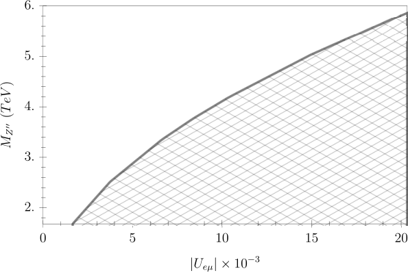
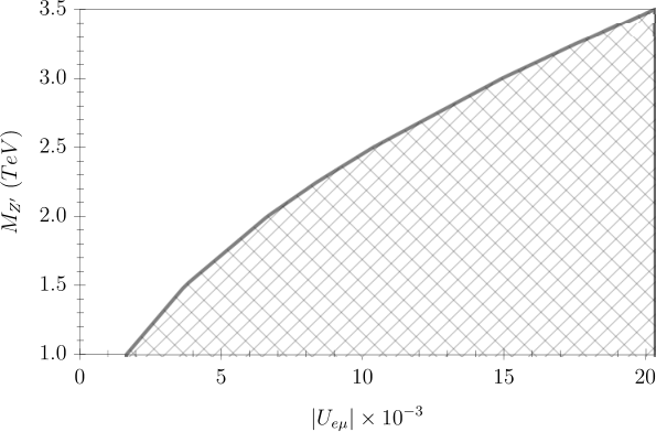
Using the experimental upper limit of the branching ratio Br​(μ⟶e​e​e¯)≤10−12\text{Br}(\mu\longrightarrow ee\overline{e})\leq 10^{-12} ref15 together with the current experimental limit Br​(μ⟶e​γ)≤10−13\text{Br}(\mu\longrightarrow e\gamma)\leq 10^{-13} ref14, we obtain, an upper limit on the lepton flavor violating matrix element |Uμ​e|≤1.66×10⁻³​MZ′2T​e​V2|U_{\mu e}|\leq 1.66\times 10^{-3}\frac{M^{2}_{Z^{\prime}}}{TeV^{2}} and a stringent bound on the gauge bosons masses MZ′≤0.597​MZ′′M_{Z^{\prime}}\leq 0.597M_{Z^{\prime\prime}}. Now if MZ′M_{Z^{\prime}}≈\approx 𝒪\mathcal{O}(1 TeV), one has |Uμ​e||U_{\mu e}|≈\approx1.66×10−31.66\times 10^{-3} and MZ′′M_{Z^{\prime\prime}}≈\approx𝒪\mathcal{O}(1.68 TeV). Figure 2 shows the variation of MZ′M_{Z^{\prime}} and MZ′′M_{Z^{\prime\prime}} as a function of |Uμ​e||U_{\mu e}| and the dashed areas represent the allowed region where the constraints are verified.
Refer to caption
Refer to caption
Figure 2: The variation of MZ′M_{Z^{\prime}} and MZ′′M_{Z^{\prime\prime}} as a function of |Ue​μ||U_{e\mu}|.

6 Conclusion

In this work, we have constructed a new unique model based on the gauge group S​U​(3)⊗S​U​(4)⊗U⁡(1)SU(3)\otimes SU(4)\otimes U(1) called the flipped 341 model where all the three quarks families arrange in the same representation whereas leptons generations are not. The anomalies cancellation requires the introduction of new extra exotic leptons a 10 plet ψe\psi_{e} and a quadruplet ψ~\widetilde{\psi}.
In the flipped 341 model, a dangerous flavor changing neutral current can appear in the lepton sector through the interactions with the neutral gauge bosons Z′Z^{\prime} and Z′′Z^{\prime\prime}, whereas, it is absent in the quark sector which makes this model unable to explain the anomalies of both kaon and B decays ref8 in contrast to the ordinary versions of the 341 models. The comparison of our results with the experimental data concerning the branching ratios of the two processes μ⟶e​e​e¯\mu\longrightarrow ee\overline{e} and μ⟶e​γ\mu\longrightarrow e\gamma lead to a stringent constraint on the matrix element and on the masses of the gauge bosons.

Acknowledgments

We would like to thank Prof. Renato M. Fonseca for fruitful discussions. We also thank Uladzimir Khasianevich for useful and clarifying comments. We are very grateful to the Algerian ministry of higher education and scientific research and DGRSDT for the financial support.

References

  • (1) A. G. Dis, P. R. D. Pinheirob, C. A. de S. Pires and P. S. Rodrigues da Silva, A compact 341 model at TeV scale, Ann.Phys.349, 232 (2014), arXiv:1309.6644 [hep-ph].
  • (2) N.Mebarki, M.Djouala, J.Mimouni and H.Aissaoui, A New Compact 341 Model: Higgs Decay Modes, FISICPAC-2018 - University of Sharjah - UAE,11-13 November 2018.
  • (3) M.Djouala and N. Mebarki, Diphton Higgs decays in the compact 341 model, 2n​d2^{nd} JIPC conference, 14-15 December 2016, Constantine, Algeria.
  • (4) M.Djouala and N. Mebarki, Exploring the Higgs Bosons in the Compact 341 Model, 1s​t1^{st} Mediterranean Conference on Higgs Physics, 23-26 September 2019, Tangier-Morocco.
  • (5) J.M.Cabarcas and J.A.Rodriguez, Electric charge quantization in models, Mod. Phys. Lett. A29, 1450032 (2014), arXiv:1303.5332 [hep-ph].
  • (6) William A. Ponce and Luis A. Sanchez, Systematic study of the S​U​(3)c⊗S​U​(4)L⊗U​(1)XSU(3)_{c}\otimes SU(4)_{L}\otimes U(1)_{X} gauge symmetry, Int. J. Mod. Phys. A,, Issue 06, pp. 435-447 (2007), arxiv:0607175 [hep-ph].
  • (7) F.Pisano and V.Pleitez, model for the electroweak interactions, Phys.Rev.D51 , 3865, (1995), arXiv:9401272 [hep-ph].
  • (8) A.Jaramiloo and L.A.Sanchez, FCNC, CP violation and implications for some rare decays in an extension of the standard model, Phys.Rev.D84.115001, (2011) arXiv:1110.3363 [hep-ph].
  • (9) R. M.Fonseca and M. Hirsch, A flipped 331 model, JHEP08, 003 (2016), arxiv:1606.01109 [hep-ph].
  • (10) N.Yamatsu, Finite dimensional Lie algebras and their representations for unified model building, arXiv:1511.08771 [hep-ph].
  • (11) S. Descotes-Genon, M. Moscati and G. Ricciardi, Non-minimal 331 model for Lepton Flavour Universality Violation in b⟶s​l​lb\longrightarrow sll decays, PhysRevD.98.115030, arXiv:1711.03101 [hep-ph]
  • (12) H.N.Long, L.T.Hue and D.V.Loi, Electroweak theory based on S​U​(4)L×U​(1)XSU(4)_{L}\times U(1)_{X} gauge group, Phys.Rev. D94 (2016) no.1, 015007, arXiv:1605.07835[hep-ph].
  • (13) W.A.Ponce and L.A.Sanchez, Systematic study of the gauge symmetry, Mod.Phys.Lett.A22, 435 (2007), arXiv:0607175 [hep-ph].
  • (14) D.T.Huong, D.N.Dinh, L.D.Thien, and P.Van Dong, Dark matter and flavor changing in the flipped 3-3-1 model, JHEP08, 051 (2019), arXiv:1906.05240 [hep-ph].
  • (15) Duong Van Loi and Phung Van Dong, Kinetic mixing effect in noncommutative B−LB-L gauge theory, JHEP09, 054 (2019), arXiv:1906.10577 [hep-ph].
  • (16) M. Tanabashi et al. (Particle Data Group), Phys. Rev. D98, 030001 (2018).
  • (17) S. Descotes-Genon, M. Moscati and G. Ricciardi, Non minimal 331 model for lepton flavor universality violation in decays, Phys.Rev.D98, 115030 (2018).
  • (18) R.Mohanta, Effect of FCNC mediated Z boson on lepton flavor violating decays, Eur.Phys. J. C71, 1625 (2011), arXiv:1011.4184[hep-ph] .