-Plane Zeros of the Potts Partition Function
on Diamond
Hierarchical Graphs
Abstract.
We report exact results concerning the zeros of the partition function of the Potts model in the complex plane, as a function of a temperature-like Boltzmann variable , for the ’th iterate graphs of the Diamond Hierarchical Lattice (DHL), including the limit . In this limit we denote the continuous accumulation locus of zeros in the planes at fixed as . We apply theorems from complex dynamics to establish properties of . For (the zero-temperature Potts antiferromagnet, or equivalently, chromatic polynomial), we prove that crosses the real- axis at (i) a minimal point , (ii) a maximal point (iii) , (iv) a cubic root that we give, with the value , and (v) an infinite number of points smaller than , converging to from above. Similar results hold for for any (Potts antiferromagnet at nonzero temperature). The locus crosses the real- axis at only two points for any (Potts ferromagnet). We also provide computer-generated plots of at various values of in both the antiferromagnetic and ferromagnetic regimes and compare them to numerically computed zeros of .
PACS numbers: 02.10.Ox,05.45.Df,64.60.De,64.60.al
1. Introduction
We derive some exact results concerning the zeros in the complex plane of the partition function, , for the -state Potts model on Diamond Hierarchical Graphs at various fixed values of a temperature-like Boltzmann variable . We also derive exact results concerning the continuous accumulation set of these zeros on the limiting Diamond Hierarchical Lattice , again at various fixed values of , and we present computer-generated images of these loci.
The Diamond Hierarchical Graphs are defined by starting with a graph consisting of two vertices (sites) and an edge (bond) joining them. The iterative graphical transformation replaces this single edge by four edges and two additional vertices, as shown in Fig. 1, yielding the next iterate, (which has the appearance of a diamond, whence the name). Fig. 1 also shows the next iterate, . We shall use the term Diamond Hierarchical Lattice (DHL) to refer to the (formal) limit . It is a self-similar, fractal object.
We recall the procedure for calculating the Hausdorff dimension of a hierarchical lattice . If the renormalization-group (RG) transformation reduces the length of each edge by a blocking factor of and gives rise to copies of the original graph, then , so [1, 2] . In the case of the iteration procedure for DHL, one has and , yielding the well-known result that
| (1) |
For this reason, we interpret the Diamond Hierarchical Lattice as being two-dimensional. (See also [3, Appendix E.3] for an interpretation of the Diamond Hierarchical Lattice as an anisotropic version of the lattice.)
The -state Potts model has been of longstanding interest in the area of phase transitions and critical phenomena. On a graph , the partition function of this model, denoted , is a polynomial in two variables, and
| (2) |
In the original statistical physics formulation, is a positive integer specifying the number of possible values of a classical spin defined at a given site of a lattice, , and is a non-negative temperature-like Boltzmann variable. (Throughout this paper we will primarily use the variable because certain expressions are simpler in rather than .) As is evident from the expression (7) given below for this partition function, it is a polynomial in both and , and one can generalize both of these variables to complex values. Indeed, this generalization is necessary when analyzing the zeros of the partition function in the plane for a given value of and in the plane for a given value of .
Part of the interest in the Potts model partition function stems from the fact that it is equivalent to a function of central importance in mathematical graph theory, namely the Tutte polynomial, (see Eq. (15) below). For some basic background on graph theory and the Tutte and chromatic polynomials, see, e.g., [4]-[9].
On a family of -vertex lattice graphs, as , an infinite subset of the zeros of merge to form certain continuous loci. In this limit, we denote the continuous accumulation locus of zeros of
- (i)
in the complex plane, for a given , as , and
- (ii)
in the complex plane, for a given , as .
In this paper we will primarily be interested in the -plane loci , however it will occasionally useful to relate them to the -plane loci and to discuss similarities and differences between these loci.
Although no exact closed-form expression for with general and , or for the corresponding dimensionless reduced free energy has been obtained on (the thermodynamic limit of) any regular lattice graph of spatial dimension , it has been possible to characterize the renormalization group (RG) action for the model exactly on certain hierarchical lattice graphs, including the Diamond Hierarchical Graphs. By performing a sum over spins at each iterative step, one can construct an exact RG transformation relating to , where is related to according to a function or equivalently, , (see Eqs. (20) and (21) below). This result follows because of the self-similarity of the Diamond Hierarchical Lattice. The properties of this model in the limit are then determined by the properties of the iterated function or equivalently . The properties of iterated analytic functions have been of considerable importance in mathematics (e.g., [10]-[11] and physics [12]-[13]). As will be clear, there are also interesting connections with complex analysis (see, e.g., [15]).
There have been many studies of spin models on hierarchical lattices, including [14]-[39], which primarily analyze the zeros of in the complex plane of the temperature-like Boltzmann variable . (A notable exception is [3] where the Lee-Yang (complex magnetic field) and Lee-Yang-Fisher (complex magnetic field and complex simultaneously) zeros are studied for the Diamond Hierarchical Lattice.) It was natural for these previous works to focus on the -plane zeros and their continuous accumulation set as , , for a given , because it is directly related to the iteration of the RG transformation at fixed value of the parameter . Indeed, (in most settings) is the Julia set in the plane for the mapping .
Considerably less attention has been paid to the zeros of in the plane and their continuous accumulation set as , , at fixed values of . Rather than being the Julia set of a rational mapping, is related to the parameter dependence of the iterates of for the fixed choice of initial condition . (This will be elaborated in Section 5.) We have noted above the study of the zeros in the plane for the Sierpinski gasket [38]. In the case of the Diamond Hierarchical Lattice the locus has been recently studied in [34], [39], and [40]. Wang, Qui, Yin, Qiao, and Gao [34] and Yang and Zeng [39] proved that the bifurcation locus for the renormalization mapping given in Eqn. (19) is connected. In Ref. [40], Chio and Roeder use techniques from complex dynamics to show that for the DHL and, in particular to prove for the DHL that the Hausdorff dimension of is 2. The paper [40] also provides a quantitative description of the limiting behavior of the chromatic zeros in terms of measure theory.
In this paper we will study properties of the loci at various choices of , beyond the case of the chromatic zeros . Using techniques from complex dynamics similar to those in [40], we will make computer images (see Figures 3 - 12) of these loci, which we relate to numerical computations of the 172 zeros of . We will also rigorously determine properties of the intersection between and the real -axis. The latter results are new even in the case of the chromatic zeros . We will also make use of results from statistical mechanics to gain further insight into the properties of .
This paper is organized as follows. In Sections 2-4 we review some relevant background on the Potts model, the family of Diamond Hierarchical Graphs, , and the iterative RG transformation that relates to . In Section 5 we present some necessary background in complex dynamics and use it to relate the locus to the “active parameters” for the RG transformation. In Sections 6 and 7 we present our results on zeros of the partition function in the plane for the Potts antiferromagnet at zero and finite temperature, respectively. We also state Theorem 7.1 describing the intersections of with the real -axis in this regime (). In Section 8 presents results on the zeros in the plane for the Potts ferromagnet, including the statement of Theorem 8.1 describing the intersections of with the real -axis in this regime (). Section 9 is devoted to proofs of Theorems 7.1 and 8.1. Section 10 contains our results on partition function zeros in the plane for various values of . Our conclusions are summarized in Section 11, and some auxiliary information is given in Appendix A.
2. Background from Graph Theory and Statistical Physics
In this section we discuss some relevant background from graph theory and statistical physics. A graph is defined by its set of vertices (= sites) and its set of edges (= bonds). We denote and as the number of vertices and edges of . At temperature , the partition function of the -state Potts model is given by
| (3) |
with the Hamiltonian
| (4) |
Here, the sum is taken over all edges of , with and labeling vertices of ; is an assignment of classical spins to the vertices; ; is the spin-spin interaction constant; and is the Boltzmann constant [41]. Further, is the Kronecker delta function. We define the notation
| (5) |
The signs of favoring ferromagnetic (FM) and antiferromagnetic (AFM) spin configurations are and , respectively. Hence, the physical ranges of are for the Potts ferromagnet (FM) and for the Potts antiferromagnet (AFM). The partition function for the -state Potts model can equivalently be written as
| (6) |
Thus is invariant under a global symmetry that acts on the spins, namely for any permutation of we can apply the mapping to the spin at each site , leaving unchanged. At high temperatures, this symmetry is realized explicitly in the physical states, while in the (thermodynamic) limit on a lattice graph with dimensionality greater than a lower critical dimensionality, it can be broken spontaneously with the presence of a nonzero long-range ordering of the spins. This ordering is ferromagnetic or antiferromagnetic, depending on the sign of .
A spanning subgraph of is with . The number of connected components of is denoted . The partition function of the Potts model can equivalently be expressed in a purely graph-theoretic manner as the sum over spanning subgraphs [42]
| (7) |
Eq. (7) shows that the partition function is a polynomial in and with positive integer coefficients for each nonzero term. As is evident from Eq. (7), has degree in and in , or equivalently, in . Furthermore, Eq. (7) allows one to generalize the parameter beyond the positive integers, . In particular, for the ferromagnetic case , Eq. (7) allows one to generalize from the positive integers to the positive real numbers while keeping a Gibbs measure, i.e., keeping . (This is not, in general, possible for the antiferromagnetic case, except when is an integer, so one can revert to the Hamiltonian formulation in Eq. (4) and (6), since is negative, so contains terms of both signs.) More generally, Eq. (7) allows one to generalize both and from their physical ranges to complex values, as is necessary in order to analyze the zeros of in for fixed and the zeros of in for fixed . Since the coefficients in are real (actually in , but all we use here is the reality), it follows that for real , the zeros of in the plane are invariant under complex conjugation and for real , the zeros of in the plane plane are invariant under complex conjugation. Since for all , it follows that always contains an overall factor of . We can thus define a reduced partition function
| (8) |
which is also a polynomial in and
Let us denote as the formal limit, as on a family of graphs (here, ). In this limit, the dimensionless, reduced free energy, per vertex, is defined as
| (9) |
(The actual free energy is equal to .) For the Potts antiferromagnet, means and thus . As is clear from Eq. (6), the only spin configurations that contribute to in this limit are those for which the spins on adjacent vertices are different. Hence,
| (10) |
where is the chromatic polynomial, which, for , counts the number of ways of assigning colors to the vertices of subject to the condition that no two adjacent vertices have the same color (called proper -colorings of ). The minimum integer that allows a proper -coloring of is the chromatic number, . Since is bipartite, . Since always contains a factor of , we also define
| (11) |
Besides its intrinsic interest in mathematical graph theory, the chromatic polynomial is important for physics because of its connection with ground-state entropy. For a family , in the limit (and hence ), the configurational degeneracy per site (vertex) of the Potts antiferromagnet is
| (12) |
For real , can be negative; in this case, since there is no obvious choice for which of the roots of to pick, one can only determine [43]. For a set of special values, , the limits and do not, in general, commute for , so one must specify the order of limits in defining [43, 44]. The set depends on the family but usually includes and . Here we define the order of limits as first and then . For a wide class of families, if is sufficiently large, then the number of proper -colorings of grows exponentially with and , so that and hence the Potts AFM has nonzero ground-state entropy per vertex on , .
The Tutte polynomial, denoted , of a graph is defined by
| (13) |
where, as above, denotes the number of connected components of the spanning subgraph , and denotes the number of linearly independent circuits on , given by . With , as defined in Eq. (5) and
| (14) |
it follows that
| (15) |
Thus, the partition function of the Potts model is equivalent, up to the indicated prefactor, to the Tutte polynomial on a given graph .
Zeros of in for a given and in for a given are of interest partly because for many families of graphs, such as strips of regular lattices, in the limit, an infinite subset of these respective zeros typically merge to form certain continuous loci. As stated above, for a one-parameter family of graphs , we define the locus as the continuous accumulation set of zeros of in the complex plane as for a fixed complex value . (There may also be discrete zeros that do not lie on this locus.) Similarly, we define the locus , or equivalently, , as the continuous accumulation set of zeros of in the complex plane of the temperature-dependent variable , or equivalently, , as for a fixed complex value [44].
For infinite-length, finite-width strips of regular lattices, and also chain graphs, is generically comprised of real algebraic curves, including possible line segments [43]-[61] (for a review and further references, see [62]). The underlying reason for this is that , and more generally, , for these classes of graphs consist of a sum of ’th powers of certain algebraic functions, denoted generically as , where is the length of the strip, and the continuous loci occur at values of where there are two or more functions that are largest in magnitude and degenerate in magnitude. An early mathematical analysis of this sort of behavior was given in [46, 45]. The Tutte polynomials for such strip graphs satisfy certain recursion relations [63]. The loci may be connected, as, e.g., for the limit of the circuit graph and strips of the square, triangular, and honeycomb lattices with periodic or twisted periodic (Möbius) longitudinal boundary conditions, and corresponding strips with toroidal or Klein-bottle boundary conditions [47],[43]-[57]. These generically separate the plane into different regions. For infinite-length limits of strip graphs and chain graphs with periodic longitudinal boundary conditions, crosses the real axis at a maximal point denoted , as well as at one or more other points [43]. If , this corresponds to the property that for this value of , passes through , signifying that the Potts antiferromagnet with has a critical point on . For a wide class of families of graphs, also crosses the real axis on the left at , but there are self-dual families where this left crossing is shifted to [57]. In contrast, for infinite-length limits of lattice strip graphs with free longitudinal and transverse boundary conditions, consists generically as (complex-conjugate pairs of) arcs and possible real line segments that do not separate the plane into different regions [64]. In all of these cases, the Hausdorff dimension of is 1. The result proved in [40] that the Hausdorff dimension of is 2 for the Diamond Hierarchical Lattice, thus provides an interesting contrast with the behavior of for these other infinite- limits of families of graphs.
The locus is commonly also comprised of curves and possible line segments in the plane. Although this is common behavior, it is not always true; a counterexample to this was found for the Archimedean lattice, where these zeros form areas rather than curves even in the case of isotropic spin-spin interaction constants considered here [65]. These areas reduce to points where crosses the real axis.
Note that the property that crosses the real axis at a point does not imply that vanishes at the point , and similarly, the property that crosses the real axis at a point does not imply that vanishes at that point . Indeed, from Eq. (7), it is evident that is a polynomial in and with positive coefficients, and hence for fixed positive , has no zeros for any real positive , and for fixed positive , has no zeros for any real positive . The property that the continuous accumulation locus of the chromatic zeros crosses the real axis at a point also does not imply that , although here the argument is more subtle, since has terms that alternate in sign with descending powers of . The precise meaning of the statement that, for a given , the continuous locus crosses the real axis at a point is that in the limit , the zeros of approach arbitrarily close to . This type of behavior is familiar from statistical physics. For example, for the -state Potts model on the square lattice with integral one has that crosses the real axis at . This critical point separates the paramagnetic phase with with explicit symmetry from the ferromagnetically ordered phase with , in which the symmetry is spontaneously broken (e.g., [41]).
3. Diamond Hierarchical Graphs and Diamond Hierarchical Lattice
In this section we discuss further details of Diamond Hierarchical Lattice graphs and the limit . We have discussed above how one defines iteratively, starting with , the tree graph with two vertices. The numbers of vertices and edges on are
| (16) |
The degree, , of a vertex on a graph is defined as the number of edges that connect to it. (The word “degree” is thus used in two different ways, here, but this should not cause any confusion.) A -regular graph is a graph all of whose vertices have the same degree. Although and are -regular graphs with and , respectively, the graphs with are not -regular, but instead have vertices with degrees ranging from 2 to . For an arbitrary graph , the average (effective) vertex degree is
| (17) |
For the Diamond Hierarchical Graphs
| (18) |
This limit is approached exponentially rapidly as gets large.
4. RG Transformations and and their fixed points
4.1. RG Transformations
By carrying out the summation over the spins at intermediate vertices at each stage, one finds the following iterative transformation for the partition function of the Potts model on the Diamond Hierarchical Graphs [1, 16]
| (19) |
where
| (20) |
or equivalently, in terms of ,
| (21) |
The two mappings are conjugate under the change of variables . The iterative transformation (20) (or equivalently, (21)), embodies the action of the real-space renormalization group action here. Although we do not append a subscript to or , it is understood that these quantities are transformed at each iteration. We denote and as the functional composition, i.e., and , respectively, and similarly for and . Note that the transformation (20) is singular at (and equivalently, (21) is singular at ), which is a physical antiferromagnetic value of if .
For illustrative purposes, we record the expressions for for the first two values of . Note that , the circuit graph with four vertices. Elementary calculations yield
| (22) |
and
| (23) |
In passing, it may be remarked that many expressions are simpler when written in terms of instead of . This is the case for the basic Eq. (7), and, for example, consists of 5 terms when written as a polynomial in and , but 10 terms when written in terms of and . For this reason, we shall generally express our results in terms of and . However, some formulas show an interesting structure when written in terms of ; for example, is a perfect square. To keep matters simple, we will focus on the variable throughout this paper and mention the variable only when it is helpful in an explanation. In the special case , Eq. (22) and (23) yield the chromatic polynomials
| (24) |
The chromatic polynomial of any graph has a zero at , and the chromatic polynomial of any graph with at least one edge has a zero at . As we shall show, for and the limit , the zero at is isolated, while the zero at occurs at one of the points where the continuous locus crosses the real axis.
The explicit expressions for become cumbersome to work with by hand for , but computer algebra systems can work with them and solve for the zeros of (fixed ) and of (fixed ) for , at which point they become polynomials of degree and , respectively. (Plots of such zeros are shown on the right-hand sides of Figures 3-16).
4.2. Preservation or reversal of the sign of
It will be convenient to write as the product of one factor, , that is positive-semidefinite for real values of and , times another, that can have either sign:
| (25) |
where
| (26) |
A basic question that one can ask about the RG transformation is whether it keeps the sign of invariant or reverses it. Recall that the physical ranges of are for the ferromagnetic sign, , and for the antiferromagnetic sign, , with corresponding to or infinite temperature, . Clearly, this transformation maps to . For nonzero , as is evident from Eq. (20), the sign of is determined by the sign of the factor . Now, with and real,
| (27) |
For physical values, the inequality (27) holds for all ferromagnetic couplings, i.e. for all . However, the situation is different for antiferromagnetic couplings, i.e., . As decreases from 0 to , the right-hand side of the inequality in (27) increases from 0 to 3/2. So for , which includes the usual integer values , is positive, so the RG transformation maps an antiferromagnetic to a ferromagnetic . Further iterations of this RG transformation keep the coupling ferromagnetic. It should also be noted that if one considers values down to, and including, , then one must take account of the fact that as decreases through AFM values to , diverges. This divergence occurs in the physical AFM interval if , which includes the integer values 1 and 2. In particular, for the (Ising) case, maps the limit for the AFM (i.e., ) to the FM (). For , a small real positive value of is mapped by to a value that is smaller than (and positive). Thus, for small positive , each iteration yields a smaller and hence a higher temperature, so that the fixed point is .
4.3. RG Fixed Points
A particularly important set of values of is the set left invariant by the transformation, i.e., the values that are RG fixed points. Here we will focus on those fixed points occurring for real values of and . They are obtained by solving
| (28) |
for the variable in terms of the parameter . Two fixed points, namely
exist for every choice of . The fixed point at corresponds to infinite-temperature (equivalently, zero-coupling), where the spin-spin interaction has no effect. The fixed point can be interpreted as meaning , and it corresponds to zero temperature (equivalently infinite-coupling) in the ferromagnetic case.
Besides the fixed points at and , solutions to the fixed point equation (28) correspond to values of satisfying the following cubic equation
| (29) |
The nature of the real roots of a cubic equation depend on the sign (or vanishing) of its discriminant (see, e.g., [67]): (i) if , then all of the roots of Eq. (29) are real; (ii) if , then Eq. (29) has one real root and a complex-conjugate pair of roots; (iii) if , then at least two of the roots of Eq. (29) coincide. For Eq. (29), the discriminant is
| (30) |
Let us consider the possibilities as increases from negative to positive values:
- (i)
For we have and (29) has one real root and a complex-conjugate pair of non-real roots. In particular, for these values of , the RG transformation has only one additional fixed point (other than ).
- (ii)
For , Eq. (29) has a triple root at , which therefore coincides with the fixed point of already discussed at the beginning of this subsection. (Note that the degree of drops from to at this parameter value, producing a dramatic change in the mapping.)
- (iii)
For , we have , and (29) has three real solutions, corresponding to three additional real fixed points of .
- (iv)
For , Eq. (29) factorizes as and thus has as solutions. Hence, has these values as fixed points.
- (v)
For we again have , and so the same description as Case (i) applies.
We summarize this discussion with Figure 2.
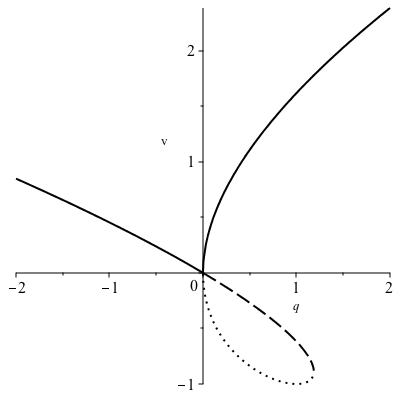
The additional fixed points of have a special interpretation when . The fixed point at is the critical value of for a Potts ferromagnet with this value of , and the double root at corresponds formally to a finite-temperature antiferromagnet. We use the word “formally” here, because for non-integral the partition function of the Potts antiferromagnet does not, in general, define a Gibbs measure and hence a normal statistical physics system.
Let us first discuss the case where and focus on the real root of Eq. (29). This root occurs as a positive value that we denote as . If is an integer , then, in the limit, there is a phase transition at , i.e., at the temperature
| (31) |
from a paramagnetic (PM) phase with manifest symmetry at high-temperatures , i.e., , to a low-temperature phase with ferromagnetic (FM) long-range order (magnetization) and associated spontaneous symmetry breaking of the symmetry to for , i.e., . We can generalize this to a phase transition from a paramagnetic to ferromagnetic phase for not restricted to integers but instead taking on any real value , since, as discussed above, defines a Gibbs measure for real positive and .
We recall that, on a regular lattice (in the thermodynamic limit), a standard Peierls argument can be used to prove that a discrete spin model without frustration, competing interactions, disorder, or dilution has a finite-temperature phase transition if the spatial dimension of the lattice is greater than the lower critical dimensionality, . Although a fractal lattice is not a regular lattice in the conventional sense, arguments have been given [1, 2] that if the Hausdorff dimensionality of the fractal lattice (in the limit) is greater than , then a discrete model (without frustration, competing interactions, disorder, or dilution) will also have a finite-temperature phase transition on the fractal lattice. This conclusion applies to our present case, since the Hausdorff dimension given in Eq. (1) is greater than 1. On a regular lattice, the PM-FM phase transition in the -state Potts model is second order, with a divergent correlation length, if and first-order, with a nonzero latent heat, if (e.g., [41] and references therein). As discussed above, in this FM case, one can generalize here from positive integers to positive real numbers for the ferromagnetic case while retaining a Gibbs measure, and one may assume this generalization here. In the limit , one must take account of a relevant noncommutativity [44]; one can define a nonvanishing free energy if one takes first, and then , and with this order of limits, there is again a second-order phase transition. An alternate approach to the case is to deal with the reduced partition function, .
For , the physical root of Eq. (29) is given by (the real, positive number)
| (32) |
with
| (33) |
where the discriminant was given in Eq. (30). The corresponding physical temperature is given by Eq. (31). The expression for in Eq. (32) is a monotonically increasing function of for . This is understandable physically, since the larger is, the more statistical fluctuations there are, so one must cool the system to a lower temperature, i.e., a larger value of and hence , for it to undergo the phase transition to a phase with ferromagnetic order. In addition to the special values and for which Eq. (29) factorizes into three linear factors, there are also values of for which it factorizes into a linear factor times a quadratic factor in , so that the expressions for all of the roots simplify considerably. For example, for , Eq. (29) factorizes as , with solutions ; for , Eq. (29) factorizes as , with solutions ; and so forth for certain larger values of . We list some illustrative values of in Table 1.
| 1 | |
|---|---|
| 32/27 | 16/9 = 1.7777… |
| 2 | 2.3830 |
| 3 | 3 |
| 4 | 3.5386 |
| 5 | 4.0261 |
| 16 | 8 |
For our analysis, we also display the other two solutions in of the cubic equation (29),
| (34) | |||||
| (36) |
where the subscripts correspond to the signs in front of the factor of . Although we initially chose to be the unique root of Eq. (29) for , the formula (32) uniquely determines a fixed point of for all , which we will continue to refer to as . We remark that, extending to complex values, as .
We refer the reader to Figure 2 where the three fixed points and are labeled for varying . Remark that they are ordered by
for those where all three exist and are distinct, i.e. for .
The effect of the RG transformation Eq. (20) on can thus be explained physically. For the high-temperature region of the ferromagnet, , i.e., the interval range , the RG transformation Eq. (20) maps the initial value of to a smaller value of , with the RG fixed point being at , i.e., . This is the standard attractive infinite-temperature fixed point of the real-space renormalization group in statistical physics and reflects the fact that a critical point is a repulsive fixed point of the RG in the temperature direction. In turn, this is a consequence of the fact that the real-space RG blocking transformation with a blocking factor of reduces the correlation length as , which is reduced finally to at . If, in contrast, the initial (real) value of the temperature is less than , i.e., is greater than , then the RG transformation Eq. (20) maps to a larger value of , with the RG fixed point in this phase being the zero-temperature fixed point where again the correlation length (defined by the connected spin-spin correlation function) vanishes.
We remark that since is bipartite, the PM-AFM critical point is given by , i.e., . As increases above 32/27, the other two roots of Eq. (29), which formed a double root at , bifurcate into a complex-conjugate pair of roots, which move to the upper and lower left away from the real axis. Asymptotically,
| (37) |
As noted above, for values of in the interval , Eq. (29) has three real roots. As decreases below the value 32/27, the real root decreases below 16/9, and the double root at bifurcates into two real roots, with decreasing and increasing as decreases toward . When reaches 1, Eq. (29) factorizes as with solutions and . Of these solutions, the first, , corresponds formally to the Potts antiferromagnet; the second, , corresponds to a finite-temperature Potts antiferromagnet, and the third, , corresponds to a finite-temperature Potts ferromagnet.
5. Rigorous Results from Complex Dynamics
In order to prove rigorous results about the continuous accumulation loci for various values of the temperature-like Boltzmann variable and to make computer pictures of it, we will need some results from complex dynamics. We will first describe them in a general context and then specialize to the case of the renormalization mapping .
5.1. Generalities on marked points and the passive/active dichotomy.
Let denote a family of rational mappings of the Riemann Sphere depending holomorphically on a complex parameter . For our purposes, is an open subset of the complex plane . Let be a choice of initial condition for the iterates of that depends holomorphically on the parameter . It is called a “marked point”, and historically [72, 73] this theory was used for marked points that are critical points of the rational mapping, in order to understand bifurcations of the mapping itself. We remark that none of the results presented in this subsection are new, and the proofs presented below are adaptations of those from the classical papers to our current context and notations.
Following the terminology of McMullen [74], the marked point is “passive” at parameter if there is an open neighborhood of on which the the sequence of functions forms a normal family, in the sense of Montel’s Theorem (see, e.g., [15] and references therein). As before, the notation denotes functional composition, , and so forth for higher .
The set of all passive parameters is open and is called the passive locus for the marked point . If the marked point is passive at the parameter , then the behavior of the initial condition does not change much as varies in a small neighborhood of . A parameter value is defined as “active” if it is not passive. At these active parameter values, the initial condition undergoes quite different dynamical behavior as is varied. Roughly speaking, this is analogous to the notion of bifurcation in the theory of dynamical systems, but the global behavior of the mapping need not change at , even if the marked point is active at . One can also think of the passive locus as a “parameter space analog of the Fatou set” that is associated to the marked point and the active locus as a “parameter space analog of the Julia set” that is associated to the marked point [76].
Let us describe a simple way for a parameter to be active. Suppose that is a repelling fixed point for . Then can be holomorphically continued to be a repelling fixed point of for all in some neighborhood of . One says that “ maps the marked point non-persistently onto the repelling fixed point at parameter ” if
In this case, it is easy to show that is an active parameter for the marked point under . (The same holds if maps the marked point “non-persistently” onto a point from a repelling periodic cycle at parameter .)
Lemma 5.1.
The set of active parameters of the marked point under the mapping contains no isolated points.
Proof.
Suppose that is an active parameter and is any neighborhood of . Since repelling periodic points are dense in the Julia set we can choose a repelling periodic cycle of period for that is disjoint from . Restricting to a smaller neighborhood of , if necessary, we can suppose that this periodic cycle varies holomorphically as
| (38) |
forming a repelling cycle of period of for all . Since is active, Montel’s Theorem implies that there is some parameter and some iterate such that for some . Since for all we see that maps the marked point non-persistently onto the repelling periodic cycle from Eq. (38) at parameter . Therefore, is another active parameter. ∎
Recall that a point is “exceptional” for a rational map if the cardinality of the set is one or two. A marked point is “persistently exceptional” for a holomorphic family of rational maps if for every parameter the point is exceptional for .
The key statement we need from holomorphic dynamics is the following simple lemma:
Lemma 5.2.
Suppose is a holomorphically varying family of rational maps, that and are marked points, and that is not persistently exceptional for .
Then, if is an active parameter for under we have
The proof is classical, but we include it here for the convenience of the reader, closely following [75, Proposition 3.5].
Proof.
Suppose for contradiction that is active under at parameter and that there is some neighborhood of such that
| (39) |
Since is not persistently exceptional, there is some such that contains points for all but finitely many possible values of , for which it has fewer than points. If is not one of those values, we can work in sufficiently small neighborhood of over which consists of disjoint graphs of holomorphic functions of . Together with Assumption (39) and Montel’s Theorem, this implies that forms a normal family on , contrary to the hypothesis that is active.
If it happened that is one of the finitely many parameters for which has fewer than points, then we use the fact that active parameters are not isolated (Lemma 5.1) to replace with another active parameter for which has the maximal number of preimages . We then apply the reasoning from the previous paragraph to the new active parameter . ∎
The following general classification of the types of behavior of a marked point for the case in which is in the passive locus will be helpful for our discussion:
Dujardin-Favre Classification of Passivity Locus [71, Theorem 4].
Let be a holomorphic family and let be a marked point. Assume is a connected open subset where is passive. Then exactly one of the following cases holds:
- (i)
is never preperiodic in . In this case the closure of the orbit of can be followed by a holomorphic motion.
- (ii)
is persistently preperiodic in .
- (iii)
There exists a persistently attracting (possibly superattracting) cycle attracting throughout and there is a closed subvariety such that the set of parameters for which is preperiodic is a proper closed subvariety in .
- (iv)
There exists a persistently irrationally neutral periodic point such that lies in the interior of its linearization domain throughout and the set of parameters for which is preperiodic is a proper closed subvariety in .
We do not include a proof of this rather difficult theorem.
5.2. Application to and the -plane zeros .
We will now explain how to use the techniques from the previous subsection to study the -plane zeros for the DHL. (The reader may wish to compare this discussion with that from [40], but note that in that paper the variable is used instead of the equivalent variable .)
Recall that is always a zero for . The renormalization procedure from Eqs. (19) and (20) implies that for any and any we have
where
is the renormalization mapping (20). Therefore, for our purposes, the marked point will correspond to the desired choice of -plane and will be constant: . (For example will correspond to the case of chromatic zeros.) Meanwhile, the other marked point will be .
We remark that the degree of drops from to when due to the appearance of a common factor of in the numerator and denominator. This is the only parameter where such a drop in degree occurs, and therefore, is a holomorphic family of rational maps with parameter space . In fact, the entire discussion in the remainder of this section will only pertain to .
For any let us denote the active locus of the marked point by .
Lemma 5.3.
Within we have .
Proof.
When we have (four different values), so that is not persistently exceptional for . Therefore, Lemma 5.2 implies that any point of is in the accumulation set of solutions to and hence the accumulation locus of zeros for , both considered as . By Lemma 5.1, contains no isolated points, so we conclude that . ∎
We will now make some observations that will help when drawing computer pictures of and that will also help us to further relate to .
For every complex parameter we have that:
- (i)
The point is a superattracting fixed point for (i.e., and ).
- (ii)
The point is a superattracting fixed point for (i.e., and , with the derivative computed in suitable local coordinates centered at .)
Therefore, for every there is an open neighborhood consisting of initial conditions whose orbit under converges to and similarly an open neighborhood consisting of initial conditions whose orbit under converges to . These neighborhoods depend continuously on the parameter .
Let
Each is a subset of the passive parameters for the marked point and each is an open set.
Lemma 5.4.
Within we have
(Here, denotes the topological boundary.)
Proof.
The proof is similar to that of Lemma 5.1. Suppose for contradiction that and suppose there were an such that the disc were disjoint from . Then, there exist values and close to such that for all . In this case the family of holomorphic functions
| (40) |
defined on would omit the three values and . Montel’s theorem would then imply that this is a normal family on , contradicting that is active. Therefore .
Now suppose that . If were a passive parameter, then there is an such that the sequence of functions given in Eq. (40) forms a normal family on . However, contains points of , so the identity theorem for holomorphic functions implies that the sequence of functions given in Eq. (40) converges to on all of . Therefore, is in the interior of contradicting the hypothesis that . We conclude that and hence that .
Proof that is the same, so we omit it. ∎
Lemma 5.5.
For any we have that
In particular and the marked point is not persistently preperiodic. (I.e. Case (ii) of the Dujardin-Favre criterion cannot hold on any connected component of the passive locus.)
Proof.
If then the point and it satisfies , implying that . If then and it satisfies , implying that . Since both and are non-empty open subsets of the connected space , their boundaries are non-empty, implying that .
If the marked point were to be preperiodic on some connected component of the passive locus, then it would be preperiodic to the same periodic cycle for all , by the identity theorem for holomorphic functions. However, there are parameters and for which maps onto the two different fixed points and , so this is impossible. ∎
The conditions that or that are easy to check numerically on the computer, so Lemma 5.4 makes visualization of the active locus easy. See, for example, Figures 3-12.
Lemma 5.6.
Within we have that
Proof.
Over any compact there is a uniform such that for all we have that is sufficiently close to that it is not equal to . (Here we used that .) This implies that is disjoint from . The same holds for using identical reasoning. ∎
Proposition 5.7.
Within the continuous accumulation locus of zeros for as contains all parameters in the boundary of and all parameters in the boundary of (these boundaries are equal). Moreover, is disjoint from .
5.3. On the possibility that
For a given choice of it may be possible to have as a result of there being components of the passive locus for other than those in . In our computer-generated pictures (Figures 3-12) for many values of one can see subsets of points colored black, corresponding to the condition that and . Any connected component of the interior of this black subset will be a passive component for the marked point . We will see that some of these components correspond to the marked point having orbit attracted to attracting periodic orbits for other than and . For such components, one can use similar reasoning to the proof of Proposition 5.7 to rule out points of . However, the other behaviors (i) and (iv) described in the Dujardin-Favre classification of the passive locus could lead to points of that are within these black regions. (Behavior (ii) is ruled out by Lemma 5.5.)
This is similar to the situation for the continuous accumulation locus of zeros in the -plane for a fixed . So long as is not an exceptional point of it follows from Montel’s theorem the Julia set of satisfies . However, it can be possible to have . For example, this will happen if:
- (i)
has a Siegel Disc in its Fatou set (i.e. a component of the Fatou set on which is conjugate to an irrational rotation),
- (ii)
, and
- (iii)
is not equal to the unique fixed point of that is in .
Then the closure of its forward orbit of will form a simple closed curve , because the dynamics of is conjugate to an irrational rotation on . This leads to some of the iterated preimages of under accumulating on every point of , implying that .
For the -plane zeros, this issue can be handled by considering only the locus where a positive proportion of the zeros of accumulate. So long as is not an exceptional point for it is a consequence of the Lyubich and Friere-Lopes-Mañe Theorems [77, 78, 79] that . In other words, any possible zeros of occurring in the Fatou set of do so with arbitrarily small proportion, in the limit .
This quantitative approach can also be taken in the -planes. Consider the locus where a positive proportion of the zeros from accumulate. For rational (and even any algebraic number ) it is a consequence of Theorem C’ from [40] that . In other words, any possible zeros of occurring in the passive locus of for do so with arbitrarily small proportion, in the limit .
5.4. On thinking in
It is very helpful to think about the continuous accumulation loci of zeros for , , as being a single object in , with the loci being horizontal slices and being vertical slices of the same object. This allows one to gain insight about by looking at near and vice-versa.
While this is very good intuition, additional care must be taken to ensure the results are rigorous, as the following delicate example shows. It is very natural to expect that
| (41) |
However, there are some delicate situations where this potentially might not hold. Suppose that there is a component of the passive locus for the marked point under for which (Julia set for ) for all . (This would correspond to Case (i) of the Dujardin-Favre classification, since we’ve ruled out Case (ii) by Lemma 5.5.) Then, for all because .
If there are some parameters for which is in the basin of attraction of an attracting cycle of , then such parameters would form an open subset of . For any we cannot have because the Julia set and Fatou set are complementary and invariant under . We would therefore have on the open set for all . In particular, such are not in and Eq. (41) would fail.
6. Zeros in the Plane for : Chromatic Zeros
In this section we study the chromatic polynomial and its zeros in the complex plane, i.e., the chromatic zeros of and their continuous accumulation set for . The left side of Figure 3 shows a computer-generated image of the regions
Any point that is not in one of these two sets is colored black. Because the sets and are open, the set of points colored black is closed. According to Proposition 5.7, contains any point of the boundary between the white, blue, and black sets. It may contain additional points, but they are necessarily in the interior of the black set. The right side of Figure 3 shows a plot of the 171 zeros of computed numerically in Mathematica. (We have omitted the zero at , hence the subscript indicating that we consider the reduced partition function.)
According to Lemma 5.4 the interior of the black set is contained in the passive locus for the marked point under . Let us consider what happens on the connected components and of the interior of the black set that are labeled on Figures 3 and 4.
We begin with the component labeled , containing the point . It intersects the real axis in the interval . For , the fixed point given in Eq. (36) is an attracting fixed point for that differs from and . Furthermore, this fixed point can be analytically continued for all and it remains an attracting fixed point of at these values. For all the orbit of initial condition converges to , which is an example of passive behavior for this marked point.
Now consider component . We have performed numerical computer studies that indicate that for every , the RG mapping has a periodic orbit of period 3 that is attracting. For values of , the orbit of under converges to this attracting cycle.
Finally, consider component , which is the cardioid of the “baby Mandelbrot set” in the upper right corner of the left half of Fig. 3 that is also shown in a magnified view in Fig. 4. Numerical experiments show that for all , the RG mapping has an attracting periodic cycle of period 2, and that the marked point has orbit converging to it.
The complexity of this region diagram is evident, even with the finite resolution of Fig. 3. One reason for the complexity is the appearance of baby Mandelbrot sets. We show one of them in Fig. 4, corresponding to a magnified view of the region enclosed by a red box in Fig. 3. However, there are infinitely many baby Mandelbrot sets in Fig. 3. Their existence can be explained using complex dynamics renormalization theory:
Theorem 6.1 (McMullen 1997 [74]).
Suppose is a holomorphic family of rational maps and is a marked critical point for . If there is at least one parameter so that the marked critical point is active under , then the active locus for the marked critical point contains quasiconformal copies of the the Mandelbrot set (or possibly of the degree generalization thereof).
In particular, it follows from the work of Shishikura [80] that the active locus of has Haudorff dimension equal to 2.
With regard to the application of McMullen’s Theorem to our in Eq. (20) with marked point , one must note that is not a critical point for . However, is a marked critical point for , and one can check that
| (42) |
so that and have the same orbit under , which, in turn, implies that their active and passive loci are the same. Therefore, McMullen’s theorem implies that the limiting locus of chromatic zeros for the DHL has Hausdorff dimension equal to 2 and that it contains small copies of the Mandelbrot set (as seen in the figures). (This was first observed by Chio and Roeder [40, Theorem B].)
An important remark here is that it is essential that the marked point be a critical point for . So, the McMullen theorem does not apply to any of the other slices with constant that we are considering. In particular, it does not imply that the limiting locus of zeros, , for these other slices have Hausdorff dimension 2. This also explains the absence of small Mandelbrot sets in Figures 5 - 12 for .
In fact, one can prove that the activity locus for the marked point under coincides with the bifurcation locus of the mapping. This is done in Proposition 7.2 from [40] for the mapping and marked point , which correspond under conjugacy to the situation here. Therefore, the work of Wang, Qui, Yin, Qiao, and Gao [34, Theorem 1.1] and Yang and Zeng [39, Theorem 1.2] implies that the boundary between the white, blue, and black regions shown in Figure 3 is connected (see Lemma 5.4). Furthermore, because , parameters where the dynamics of bifurcates will be in . Again, this is special to the case .
We comment on several general properties. For this and the other region diagrams studied here, with both (antiferromagnetic range) and (ferromagnetic range), the outer part of the diagram, extending infinitely far from the origin, is characterized by the property that , as indicated by the white color. For real , this can be understood as follows. In both the antiferromagnetic and ferromagnetic Potts model, an increase in introduces more fluctuations in the system, since the spin at each site can take on values in a larger set. Hence, for a given temperature and hence a given value of , the system will be in the disordered phase with no long-range spin-spin ordering. The RG transformation will thus move the system toward the infinite-temperature fixed point at .
The inner part of the diagram is comprised of blue, black, and also white regions (the white regions being separated from the outer white region by parts of . An outer boundary separates the outer white region from this complex inner set of regions.
Let us now discuss some properties of how intersects the real axis. We refer the reader to Figure 3 throughout the discussion. We claim that:
- (i)
The left-most real point where intersects the real axis is ,
- (ii)
The right-most real point where intersects the real axis is , and
- (iii)
There is an infinite sequence of points where intersects the real axis converging to .
We will first give a physical description and interpretation of these properties. They will later be proved as part of Theorem 7.1.
Let us denote by the right most place where intersects the real axis. It can be explained by the fact that there is a qualitative change in the locus at , namely the appearance of an antiferromagnetic transition at [21]. Therefore, the intuitive approach that if and only if indicates that this should lead to . This expresses the property that the Potts antiferromagnet has a zero-temperature critical point on .
Note that although crosses the real axis at this point, the chromatic polynomial has the nonzero value (48) at . We remark that is equal to the value that was inferred in a similar manner for the Sierpinski gasket fractal in [38] and is also the same as the value for the (infinite) square lattice [68]. Interestingly, it is also the same as the value of that was derived for infinite-length self-dual strips of the square lattice [57].
The nature of the Julia set and hence of changes qualitatively depending on whether the discriminant (30) is positive, negative or zero, and the demarcation point between positive and negative values occurs at the special value . Connected with this, we infer that crosses the real axis at and, furthermore, that this is the minimal positive value of where such a crossing occurs. Note that the point itself is not a chromatic zero of for any . More generally, it has been proved that for an arbitrary graph, the real interval is free of chromatic zeros [69] (see also [70]).
Let us now start at the right-most crossing at and move to the left through the adjacent inner blue region. This blue region extends down to a point that is the unique real root of the cubic equation
| (43) |
namely,
| (44) | |||||
| (46) |
where crosses the real axis. Indeed, one finds that
The former implies that the marked point is active for and for so that Lemma 5.3 gives that they are in . The latter implies that (blue region); see Lemma 9.4(ii). Eqn. (46) was obtained by solving
| (47) |
whose solutions correspond to all values of for which is either a fixed point or mapped to a fixed point. Eqn. (47) has four real solutions and . (The first two solutions correspond to passive behaviors for the marked point , with it being a superattracting fixed point when and it being mapped by to the superattracting fixed point at when .)
Fig. 3 also shows a succession of regions and associated crossings of with the real axis, extending to the left of and converging on from above. Between these crossings are an infinite set of regions, alternating between blue and white, also decreasing to from above. However, the figure, calculated and presented to finite resolution, can only show a finite subset of these.
We have numerically computed the ten largest crossing points of with the real axis and we present them in Table 2. They were computed using a method similar to the computation of , described above. More specifically, for we numerically solved the equation
for within suitably chosen intervals that were deduced from Figure 3.
It is of interest to compare the exact results discussed above and depicted on the left hand side of in Fig. 3 with the chromatic zeros of calculated for finite shown on the right hand side of Fig. 3. Extensive experience with chromatic zeros of sections of regular lattices has shown that a subset of these approach the locus as the number of vertices gets large (e.g., [43], [49]-[56]). Here we observe a similar behavior, although for the diamond hierarchical lattice is obviously much more complicated than the real algebraic curves and possible line segments comprising the loci for the limits of sections of regular lattices and related chain graphs. In particular, one can see (complex-conjugate pairs of) zeros near and , as well as a clustering of chromatic zeros forming a wedge-shaped pattern, with the apex of the wedge facing left and located on the real axis at , close to . The zeros that we have calculated for graphs show considerable scatter, and in this respect they differ from the chromatic zeros that were calculated in [38] for Sierpinski graphs. From a comparison of the zeros for , we find that the left-most complex-conjugate pair of zeros move toward the point as increases, in agreement with the property deduced from the analysis leading to Fig. 3, that is a crossing of . This is consistent with the fact that in other cases (e.g. [48, 54, 44, 59, 58] where this behavior (of complex-conjugate pairs of zeros in the vicinity of moving toward the latter point as increases) is observed, and one has exact results for , it is associated with the property that for , the locus passes through and separates the complex plane into different regions.
In analyzing these chromatic zeros and their limiting behavior for , it is useful to recall some rigorous results on zero-free regions on the real axis. Since the signs of descending powers of in alternate, an elementary property is that has no zeros in the interval . For an arbitrary graph , there are also no chromatic zeros in the interval (0,1) and, as mentioned above, in the interval ; see [69], [70], [9]. Thus, although crosses the real axis at the point , this point itself is not a chromatic zero. Since always has a factor of , it always vanishes at , and if, as is the case here, has at least one edge, then also vanishes at . For , we find that the only real zeros of are . It is interesting to note that although , this polynomial can be quite small for part of the interval . For example, as increases from 1 to 2, reaches a local maximum of 0.041 at , then decreases to a local minimum of 0.0080 at , and finally increases to 2 as . In the same interval, reaches a maximum of 0.0090 at , decreases to a minimum of approximately at , and then increases to 2 at .
Let us remark on another property of . Because is bipartite, . By explicit iterative calculation, we obtain
| (48) |
Consequently,
| (49) |
so that the 3-state Potts AFM has ground-state entropy on the fractal given by
| (50) |
Interestingly, these results are the same as for the infinite-length square-lattice ladder graph (with any longitudinal BC) [43]), for which
| (51) |
and hence . The cyclic and Möbius strips of the square lattice with width vertices are -regular graphs with vertex degree , and the free square-lattice strip also has in the limit. These values of and are the same as the value (18).
7. Zeros in the Plane for the Potts Antiferromagnet at Nonzero Temperature
We next consider the zeros of for the Potts antiferromagnet with temperature which corresponds to the range . On the left sides of Figures 5 - 7 we present computer-generated images of the regions
for , and . Any point that is not in or is colored black. According to Proposition 5.7, contains any point of the boundary between the white, blue, and black sets. It may contain additional points, but they are necessarily in the interior of the set of black points.
For comparison, on the right sides of Figures 5 - 7 we present the numerically computed zeros of the reduced partition function at these values of . (As usual, the zero at is omitted.)
First, we observe that in the case of infinite temperature, or equivalently, zero spin-spin coupling, we have that for any graph , so that all of the zeros of occur at . Previous studies (e.g., [44, 58]) showed that generically, as approaches 0, the zeros of in the plane progressively move in toward the origin, . We see that behavior here for the diamond hierarchical graphs , as evident from the decreasing scale of Figures 3 and Figures 5-7 as increases from to .
Note also that for and the zeros of show somewhat less scatter than at . Moreover, one sees that the wedge-like formation of zeros moves to the left as increases, intersecting the real real axis at for , for , and at for .
As increases in the interval , there is an evident simplification in the different regions on the left side of Figures 5-7, as compared with the case. As was found for regular lattice graphs (e.g., [44]), as increases in the interval , the maximal point, , at which crosses the real axis decreases. This behavior is expected, since as , all of the zeros move in toward . The crossing at remains present for all .
Although it is not completely evident from Figures 5 - 7, for any the locus continues to intersect the real axis in infinitely many points, just like in the case . One can observe this by using the computer to zoom in when investigating the region diagrams. However, we will prove it rigorously in the theorem below.
The following theorem summarizes the antiferromagnetic case:
Theorem 7.1.
For any the locus intersects the axis at and at
The locus does not intersect the real axis at any point outside of the interval .
Furthermore, there is an infinite sequence of points where intersects the real axis converging to
| (52) |
which is also in .
We refer the reader to Figure 8 for a plot of . The values of for these values of shown in Figures 3, 5, 6, and 7 are , and , respectively. Theorem 7.1 will be proved in Section 9.

8. Zeros in the Plane for the Ferromagnetic Potts Model
We now present some results on the zeros of and the locus in the complex plane for the Potts ferromagnet, corresponding to . On the left sides of Figures 9 - 12 we present computer-generated images of the regions
for , and . As in previous figures, any point that is not in or is colored black. According to Proposition 5.7, contains any point of the boundary between the white, blue, and black sets. It may contain additional points, but they are necessarily in the interior of the set of black points.
For comparison, on the right sides of Figures 9 - 12 we present the numerically computed zeros of the partition function at these values of . (As usual, the zero at is omitted.)
In general, for all four of these ferromagnetic values of , especially for the largest two values, the region diagram appears considerably simpler than for the antiferromagnetic values. As in the antiferromagnetic case, the region diagrams have an outer white area extending infinitely far from the origin, separated from an inner blue and black portion by part of . For and there are still some black regions, but they have become rather small, and for and , at the resolution of the figures, one sees only an inner blue region and an outer white region, separated by . Furthermore, they appears to become smoother, approaching a nearly circular form for large , as will be discussed further below. The computer images also indicate that the Hausdorff dimension of decreases as increases sufficiently.
Another difference from the antiferromagnetic values of is that for the ferromagnetic values the locus intersects the real axis in only two points:
Theorem 8.1.
For any the locus intersects the real -axis only at the two points given by
We refer the reader to Figure 13 for a plot of . The values of and for these values of shown in Figures 9 - 12 are , , , and , respectively. Theorem 8.1 will be proved in Section 9.

We can give a statistical physics explanation of the crossing of on the positive real axis; the Potts ferromagnet has a phase transition at this value of for the given value of the temperature variable , namely as given in Eq. (31). For larger , the system is more disordered; for integral , this can be understood from the fact that each spin on the lattice can take values in a larger set, . In this case, the infinite iteration of the RG transformation maps the temperature to , or equivalently, decreases to 0, hence the white color. For the system is more ordered, so the infinite iteration of the RG transformation maps the temperature variable to , i.e., , hence the blue color.
In contrast with the scattered pattern of zeros in the plane for the AFM case , the zeros in the plane for the FM case illustrated by these four values of tend to cluster along a curve. This curve encircles the origin. As gets large, this curve assumes an oval-like shape. In [82] (see also the related [81]), we showed that, in the limit of a recursive family of graphs, as increases to values , the accumulation set of zeros in the plane, , forms a closed oval curve that encircles the origin and crosses the positive axis at
| (53) |
where was defined in Eq. (17). In this limit, forms a closed oval curve approaching a circle, crossing the positive and negative real axes at a value of that behaves asymptotically as
| (54) |
9. Proofs of Theorems 7.1 and 8.1.
We will consider the dynamics of the RG mapping for and .
9.1. Lemmas and setup.
Let us briefly summarize some properties of that will be used throughout this section.
For any the mapping has a superattracting fixed point at and another fixed point . Moreover, is the unique positive fixed point of for any , a property that will play an important role in several of the proofs.
For the mapping has two additional fixed points and with
When these two fixed points collide: . Figure 2 shows a plot of how , , and depend on .
The mapping has a pole at
The critical points of are:
Note that
for any .
Lemma 9.1.
The extended real interval is invariant under .
Proof.
One can check that the expression for is a perfect square. ∎
Lemma 9.2.
For any real we have that is a repelling fixed point for satisfying .
Proof.
We remark that for the fixed point is a solution to the equation that occurs with multiplicity one so that we cannot have .
Case 1: . The pole and all of the critical points of lie in . A simple calculation shows that for . Since and is the unique fixed point of occurring at positive we conclude that for and that for . Since we must have , as desired.
Case 2: . The pole at and two of the critical points and occur at positive and they do so with the following order:
Since and the Intermediate Value Theorem implies that has a fixed point between and . Since is the unique positive fixed point of we conclude that
Moreover, one can check that is positive on .
Suppose for contradiction that . Then, for
with chosen sufficiently close to , one has . Since the Intermediate Value Theorem would imply that there is an additional fixed point of with . This contradicts that is the unique positive fixed point of . Since we must therefore have . ∎
Lemma 9.3.
We have:
- (i)
If then for any we have as .
- (ii)
If is sufficiently small then for any we have as .
Proof.
Claim (i): When the pole and the critical points and occur at positive . The critical point occurs for . The only real fixed points for are and . A calculation shows that and hence that for all . Another calculation shows that for all . Therefore, the sequence is increasing sequence that is bounded above by . It must converge to some limit, which will be a fixed point for . Therefore, .
Claim (ii): Suppose and that is sufficiently small that . In this case, we have
The critical point occurs at and the other two critical points and the pole of are ordered as
We have that
so we conclude that and hence that for all . In particular, we have
This implies that for any we have ∎
Lemma 9.4.
For any real we have
- (i)
If then as ,
- (ii)
If then as .
We remark that in Claim (i) when the orbit of may pass into the interval .
Proof.
We split the proof of Claim (i) into two cases:
Case 1: . As in the first paragraph of the proof of Lemma 9.2, we have
If then the orbit forms a decreasing sequence, which is bounded below by , and hence converges. The limit must be a fixed point of and, since is the only positive fixed point of , we see that .
Case 2: . As in the second paragraph of the proof of Lemma 9.2, the critical points, pole, and fixed points of occur with the following order:
| (56) |
We will show that is invariant under and that for any we have .
The zeros of are
Since and we have . Therefore, for any we have .
Now consider . On this interval, we have . The orbit cannot remain in because, if it did, the orbit would form a decreasing sequence that is bounded below by . It would therefore converge to some fixed point of satisfying , which is impossible because is the unique positive fixed point of . Therefore, for any there is some iterate for which , at which point the reasoning in the previous paragraph implies that .
We will now prove Claim (ii). Note that pole cannot occur on ; see Eqn. (56) for the case that . Therefore, since and , by Lemma 9.2, we have that for all . (When we allow for the possibility that is the pole of .) This implies that if the sequence of iterates is increasing. It must converge to infinity as there is no fixed point of that is larger than . ∎
9.2. Proof of Theorem 8.1.
Recall from Section 4.3 that the fixed points of other than and are roots of the equation
Solving for the values of for which has a fixed point at yields the two solutions
Since we consider , the resulting fixed point will necessarily be , as it is the only positive fixed point of .
If or then and by Lemma 9.4. Therefore,
and Proposition 5.7 implies that does not intersect such points. (Such points are colored white in Figures 9 - 12.)
9.3. Proof of Theorem 7.1.
Let . Lemma 9.3(i) gives for any that and hence . Proposition 5.7 implies that does not intersect such points.
We will now show that is in . This requires some care because the degree of drops from to at . (It is why we omitted from the parameter space in the discussion from Section 5.) For this reason, Lemma 5.3 does not immediately apply to . Instead, we will show for any that there is a parameter with that is active for under . Such a point is in by Lemma 5.3, and, since is arbitrary, this will prove that .
As seen in the previous paragraph, any real point is in . Note that as the fixed point increases to ; see Figure 2. Therefore, we can choose sufficiently small so that . It then follows from Lemma 9.3(ii) that . We conclude that on any arbitrarily small annulus there are two different passive behaviors for the marked point : (i) convergence to and (ii) convergence to . Therefore, there must be active parameters in this annulus.
We will now prove that is the largest point where hits the real -axis. One finds that
which is negative for . We have
Since is positive and increasing for the Intermediate Value Theorem gives that for any there is a unique for which
In particular, when the marked point lands non-persistently on the repelling fixed point when mapped by . This implies that is an active parameter for and hence that , by Lemma 5.3.
Moreover, for . Lemma 9.4(i) then implies that such are in and Proposition 5.6 then implies that they are not in .
The formula is obtained by solving for and selecting the branch of the solutions that is larger than the pole .
It remains to show that there is a sequence of real parameters that converge to ; See Eq. (52).
Case 1: :
When a direct calculation shows that for all and as . When we have
We claim that for any the function has at least one pole in the interval . To see this, note that if has a pole , then is also a pole of since for any . Otherwise, if has no pole in the interval then
so that the Intermediate Value Theorem implies that there is some with . Since is a pole of this implies that .
For any let be the smallest pole of in the interval . We have
with the fact that the limit is (not ) a consequence of Lemma 9.1. For any the repelling fixed point remains in . Therefore, the Intermediate Value Theorem implies that there exists with
As this does not hold identically for all , we conclude that the marked point is mapped by non-persistently at . It follows from Lemma 5.3 that .
For any there is a definite constant such that
Meanwhile, for any . Therefore, there is a definite such that for any we have . Since is invariant under for and the pole is negative, this implies that for any we have
Since was arbitrary, we conclude that as .
Case 2: :
A straightforward modification of the proof from Case 1 applies, after replacing with the unique value of for which .
∎
10. Zeros in the Plane
In addition to the zeros of in the plane for fixed and their accumulation locus in the limit , it is also of interest to investigate the zeros of in the plane for fixed and their accumulation locus in this limit . We present some new results on these in this section.
As was noted in [16], these zeros form the the Julia set of the transformation [76]. This can be understood as follows. Assume that, for a fixed , is a zero of , i.e., . Then from Eqs. (19)-(20), it follows that
| (57) |
Hence, if . This connects the set of points for which to the set of values of that are left invariant by the transformation . Since a deviation of a given from this invariant set will generically be multiplied by successive iterations of , this yields the identification of with the Julia set of . Previous studies have presented zeros in the plane for low values of .
Here we extend this study of zeros of in with new results for large positive and negative values of . Although negative values of do not have direct significance for the physical -state Potts model, they are of interest in investigating the mathematical properties of the full polynomial. In [82] we showed that crosses the positive axis at
| (58) |
Since, as noted above, is close to 3 for , it follows that the zeros to cross the positive axis at for . In agreement with this, we show our calculations of zeros of in the plane for the large positive values , , and the large negative value in Figs. 14-16. (The number of zeros displayed in each of these figures, namely 256, is sufficiently great that the plotting program yields what appears to be a curve, although it is really a discrete set of zeros.)
There is a striking change in the structure of the zeros as grows to values that are [16, 21, 39]. In particular, the Hausdorff dimensionality of the Julia set approaches 1 from above asymptotically as [21, 35]. Related to this, the global pattern of zeros becomes a single Jordan curve rather than the more complicated patterns observed for small . The fact that this Jordan curve is not too different from a circle is similar to the pattern of complex-temperature zeros for the Potts model on regular lattices in the limit of large [81, 82].
11. Conclusions
In this paper we have derived several exact results on the continuous accumulation sets of zeros of the Potts model on the Diamond Hierarchical Lattice, , in the complex -plane at various fixed values of a temperature-like Boltzmann variable . We have applied methods from complex dynamics to determine the region diagram in which the infinite iteration of the renormalization group transformation exhibits different behavior in the various regions and related them to the locus . We have also used these techniques to prove rigorous results (Theorems 7.1 and 8.1) about the intersection of with the real -axis. For the chromatic zeros (i.e., partition function zeros of the zero-temperature Potts antiferromagnet), we have shown that the locus crosses the real axis at , , , and an infinite set of points between 32/27 and the value given analytically in Eq. (46). A similar behavior occurs for any finite-temperature Potts antiferromagnet on the DHL. For the finite-temperature Potts ferromagnet on the DHL, the locus crosses the real axis at only two points. We have also studied region diagrams and the structure of for the finite-temperature Potts antiferromagnet and for the Potts ferromagnet on the DHL and compared them with the patterns of zeros calculated for with . Another result of our present work is that as , approaches a circular form with . Finally, we determine properties of the locus for .
Acknowledgments: This research was partly supported by the Taiwan Ministry of Science and Technology grant MOST 103-2918-I-006-016 (S.-C.C.), by U.S. National Science Foundation grant No. NSF-DMS-1348589 (R.R.), and by the U.S. National Science Foundation grants No. NSF-PHY-1620628 and NSF-PHY-1915093 (R.S.).
Appendix A On the Case
Besides the very delicate potential issues about relating with that we discussed in Section 5.4, there is an additional problem that occurs when , which we explore it in this appendix. It is related to the more general fact that in defining the free energy from the partition function, it is necessary to take into account a noncommutativity in the limits and at special values (which may include , where denotes the chromatic number of ). This was discussed in [43] for the chromatic polynomial and in [44] for the full free energy. The noncommutativity is
| (59) |
As in the text, we denote as the formal limit of an iterative family of -vertex graphs as and hence . Because of this noncommutativity, the definitions of both the free energy in (9) and require that the order of limits be specified.
A simple example will illustrate this. Consider the Potts model on the -vertex circuit graph, . An elementary calculation yields, for the partition function, the result
| (60) |
As a special case of Eq. (7), has as a factor, so . As an explicit example of the noncommutativity (59) with ,
| (61) |
while, in contrast, if one takes the limit first, before taking , then
| (62) |
Then finally taking , one obtains
| (63) |
The loci and are given by the solution of the condition of equality of dominant terms in , namely
| (64) |
In the plane, the solution locus, , is a circle with radius . If is real, this circle is centered at and crosses the real axis at the two points and . Thus, the maximum (finite) point at which this locus crosses the real axis is
| (65) |
For example, in the case where is the chromatic polynomial and is the continuous accumulation set of the chromatic zeros, the locus is the unit circle , which crosses the real axis at and .
To show the connection with or equivalently, , with , we first note that the solution of Eq. (64) in the complex plane is the infinite vertical line crossing the real axis at , i.e.,
| (66) |
Equivalently, in the complex plane, is the infinite vertical line crossing the real axis at :
| (67) |
It is convenient to change variables to a variable in terms of which the locus is compact. We choose ; in the complex plane of the variable , if , then the locus is a circle:
| (68) |
As is evident from Eq. (68), this circle crosses the real axis at and . If , then is the line with , i.e., the imaginary axis. This locus is invariant under , so the locus is also the imaginary axis in the plane.
Here we observe that the point is in the locus for all , in particular, for , i.e., , but is not in the locus for . Explicitly, if , then is the vertical line in the plane crossing the real axis at ; equivalently, is the circle crossing the real axis at and .
References
- [1] M. Kaufman and R. B. Griffiths, Exactly soluble Ising models on hierarchal lattices, Phys. Rev. B 24 496-498 (1981); R. B. Griffiths and M. Kaufman, First-order transitions in defect structures at a second-order critical point for the Potts model on Hierarchical lattices, Phys. Rev. B 26 5022-5032 (1982); M. Kaufman and R. B. Griffiths, Spin systems on hierarchical lattices II. Some examples of soluble models, Phys. Rev. B 30 244-249 (1984).
- [2] Y. Gefen, B. B. Mandelbrot, and A. Aharony, Critical phenomena on fractal lattices, Phys. Rev. Lett. 45 855-858 (1979); Y. Gefen, A. Aharony, and B. B. Mandelbrot, Phase transitions on fractals: I. Quasi-linear lattices, J. Phys. A 16 1267-1278 (1983); Y. Gefen, A. Aharony, and B. B. Mandelbrot, Phase transitions on fractals: II. Sierpinski gaskets, J. Phys. A 17 (1984) 435-444; Y. Gefen, A. Aharony, and B. B. Mandelbrot, Phase transitions on fractals: III. Infinitely ramified lattices, J. Phys. A 17 1277-1289 (1984).
- [3] P. Bleher, M. Lyubich, and R. Roeder, Lee-Yang zeros for DHL and 2D rational dynamics: foliation of the physical cylinder, Journal de Mathematiqués Pure et Appliquée 107, 491-590 (2017) [arXiv:1009.4691]; P. Bleher, M. Lyubich, and R. Roeder, Lee-Yang-Fisher zeros for DHL and rational dynamics: global pluripotential interpretation, arXiv:1107.5764.
- [4] Biggs, N: Algebraic Graph Theory (Cambridge Univ. Press, Cambridge, 2nd ed., 1993).
- [5] Bollobás B, Modern Graph Theory (Springer, New York, 1998).
- [6] T. Brylawsky and J. Oxley, The Tutte polynomial and its applications, in N. White, ed., Matroid Applications, vol. 40 of Encyclopedia of Mathematics and its Applications (Cambridge Univ. Press, Cambridge, UK, 1992), pp. 123-225.
- [7] R. C. Read, Introduction to chromatic polynomials, J. Combin. Theory 4, 52-71 (1968).
- [8] R. C. Read and W. T. Tutte, “Chromatic polynomials”, in Selected Topics in Graph Theory, eds. L. W. Beinecke and R. J. Wilson (Academic Press, New York, 1988).
- [9] F. M. Dong, K. M. Koh, and K. L. Teo, Chromatic Polynomials and Chromaticity of Graphs (World Scientific, Singapore, 2005).
- [10] A. F. Beardon, Iteration of Rational Functions (Springer, Berlin, 1991).
- [11] J. Milnor, Dynamics in One Complex Variable, 2nd ed. (Vieweg, Berlin, 2000).
- [12] H. E. Stanley and E. Taylor, Fractals in Science (Springer, New York, 1994).
- [13] A. Bunde and S. Havlin, eds. , Fractal and Disordered Systems (Springer, Berlin, 1996);
- [14] A. N. Berker and S. Ostland, Renormalization-group calculations of finite systems: order parameter and specific heat for epitaxial ordering, J. Phys. C 12 4961-4975 (1979).
- [15] R. Remmert, Classical Topics in Complex Function Theory (Springer, New York, 2010).
- [16] B. Derrida, L. De Seze, and C. Itzykson, Fractal structure of zeros in hierarchical models, J. Stat. Phys. 33 559-569 (1983); B. Derrida, C. Itzykson, and J. M. Luck, Oscillatory critical amplitudes in hierarchical models, Commun. Math. Phys. 94, 115-132 (1984); C. Itzykson and J. M. Luck, in Progress in Physics (Birkhauser, Basel, 1985), vol. 11, pp. 45-82.
- [17] G. Bhanot, H. Neuberger, and J. A. Shapiro, Simulation of a critical Ising fractal, Phys. Rev. Lett. 53 2277-2280 (1984).
- [18] B. Hu, Problem of universality in phase transitions on hierarchical lattices, Phys. Rev. Lett. 55 2316-2319 (1985); Y.-K. Wu and B. Hu, Phase transitions on complex Sierpinski carpets, Phys. Rev. A 35 1404-1411 (1987).
- [19] B. W. Southern and M. Knežević, Zeroes of the partition function of Ising models on fractal lattices, Phys. Rev. B 35 5036-5042 (1987).
- [20] P. Bleher and E. Zalys, Asymptotics of the susceptibility for the Ising model on the hierarchical lattices, Commun. Math. Phys. 120 409-436 (1989); P. M. Bleher and M. Yu. Lyubich, Julia sets and complex singularities in hierarchical Ising models, Commun. Math. Phys. 141, 453-474 (1991).
- [21] B. Hu and B. Lin, Yang-Lee zeros, Julia sets and their singularity spectra, Phys. Rev. A 39, 4789-4796 (1989).
- [22] Y. Qin and Z. R. Yang, Diamond-type hierarchical lattices for the Potts antiferromagnet, Phys. Rev. B 43, 8576-8582 (1991).
- [23] Z. R. Yang, Solvable Ising model on Sierpinski carpets: the partition function, Phys. Rev. E 49 2457-2462 (1994).
- [24] L. de Silva et al., Criticality and multifractality of the Potts ferromagnetic model on fractal lattices, Phys. Rev. B 53, 6345-6354 (1996).
- [25] J. Qiao and Y. Li, On connectivity of Julia sets of Yang-Lee zeros, Commun. Math. Phys. 222, 319-326 (2001).
- [26] R. G. Ghulghazaryan, N. S. Ananikian, and P. M. A. Sloot, Yang-Lee zeros of the -state Potts model on recursive lattices, Phys. Rev. E 66, 046110 (2002).
- [27] Y.-L. Chou and M.-C. Huang, Distribution and density of partition function zeros for the diamond-decorated Ising model, Phys. Rev. E 67, 056109 (2003).
- [28] J. Qiao, On Julia sets concerning phase transitions, Science in China A 46, 415-431 (2003).
- [29] J. Gao and J. Qiao, Julia set concerning Yang-Lee theory, Phys. Lett. A 355, 167-171 (355).
- [30] J. Qiao, Julia sets and complex singularities in diamond-like hierarchical Potts models, Science in China A 48, 388-412 (2006).
- [31] J. Qiao and J. Gao, Jordon domain and Fatou set concerning diamond-like hierarchical models, Nonlinearity 40, 119-131 (2007).
- [32] J. De Simoi, Potts models on hierarchical lattices and renormalization group dynamics: II. Examples and numerical results, J. Phys. A 42, 095002 (2009).
- [33] J. Qiao, Y. Yin, and J. Gao, Feigenbaum Julia set of singularities of free energy, Ergodic Theory and Dynamical Systems 30, 1573-1591 (2010).
- [34] X. Wang, W. Qiu, Y. Yin, J. Qiao and J. Gao, Connectivity of the Mandelbrot set for the family of renormalization transformations. Science in China, 53, 849-862 (2010).
- [35] J. Gao, Julia sets, Hausdorff dimension and phase transition, Chaos, Solitons, and Fractals 44, 871-877 (2011).
- [36] J. Gao and J. Qiao, Continuity of Julia set and its Hausdorff dimension of Yang-Lee zeros, J. Math. Anal. Appl. 378, 541-548 (2011).
- [37] S.-C. Chang and L.-C. Chen, Spanning trees on the Sierpinski gasket, J. Stat. Phys. 126, 649-667 (2007); S.-C. Chang and L.-C. Chen, Spanning forests on the Sierpinski gasket, Discrete Math. Theor. Comput. Sci. 10, 55-76 (2008).
- [38] S.-C. Chang and R. Shrock, Zeros of the Potts model partition function on Sierpinski graphs, Phys. Lett. A 377, 671-675 (2013).
- [39] F. Yang and J. Zeng, J. Mathematical Analysis and Applications 413, 361-377 (2014).
- [40] I. Chio and R. K. W. Roeder, Chromatic zeros on hierarchical lattices, Preprint: https://arxiv.org/abs/1904.02195.
- [41] F. Y. Wu, The Potts model, Rev. Mod. Phys. 54, 235-268 (1982).
- [42] C. M. Fortuin and P. W. Kasteleyn, On the random cluster model, Physica 57, 536-564 (1972).
- [43] R. Shrock and S.-H. Tsai, Asymptotic limits and zeros of chromatic polynomials and ground state entropy of Potts antiferromagnets, Phys. Rev.E55, 5165-5179 (1997).
- [44] R. Shrock, Exact Potts model partition functions for ladder graphs, Physica A 283, 388-446 (2000).
- [45] S. Beraha, J. Kahane, and N. Weiss, Limits of zeros of recursively defined polynomials, Proc. Nat. Acad. Sci. 72, 4209 (1975).
- [46] S. Beraha, J. Kahane, and N. Weiss, Limits of chromatic zeros of some families of maps, J. Combin. Theory B 28, 52-65 (1980).
- [47] R. J. Baxter, Chromatic polynomials of large triangular lattices, J. Phys. A. 20, 5241-5261 (1987).
- [48] R. Shrock and S.-H. Tsai, Ground state degeneracy of Potts antiferromagnets on 2D lattices: approach using infinite cyclic strip graphs, Phys. Rev. E60, 3512-3515 (1999); R. Shrock and S.-H. Tsai, Exact partition functions for Potts antiferromagnets on cyclic lattice strips, Physica A 275, 429-449 (2000).
- [49] R. Shrock and S.-H. Tsai, Ground state entropy of the Potts antiferromagnet on cyclic strip graphs, J. Phys. A Letts. 32, L195-L200 (1999).
- [50] R. Shrock, partition functions for Potts antiferromagnets on Möbius strips and effects of graph topology, Phys. Lett. A 261, 57-62 (1999).
- [51] N. L. Biggs and R. Shrock, partition functions for Potts antiferromagnets on square lattice strips with (twisted) periodic boundary conditions, J. Phys. A (Letts) 32, L489-L493 (1999).
- [52] S.-C. Chang and R. Shrock, Ground state entropy of the Potts antiferromagnet on strips of the square lattice, Physica A 290, 402-430 (2001).
- [53] S.-C. Chang and R. Shrock, partition functions for Potts antiferromagnets on lattice strips with fully periodic boundary conditions, Physica A 292, 307-345 (2001).
- [54] R. Shrock and S.-H. Tsai, Ground state entropy of Potts antiferromagnets on cyclic polygon chain graphs, J. Phys. A 32, 5053-5070 (1999).
- [55] R. Shrock, Chromatic polynomials and their zeros and asymptotic limits for families of graphs, in Proc. of the 1999 British Combinatorial Conference, Discrete Math. 231, 421-446 (2001).
- [56] S.-C. Chang and R. Shrock, Ground state entropy of the Potts antiferromagnet with next-nearest-neighbor spin-spin couplings on strips of the square lattice, Phys. Rev. E 62, 4650-4664 (2000).
- [57] S.-C. Chang and R. Shrock, Potts model partition functions for self-dual families of graphs, Physica A 301, 301-329 (2001).
- [58] S.-C. Chang and R. Shrock, Exact Potts model partition functions on strips of the triangular lattice, Physica A 286, 189-238 (2000).
- [59] S.-C. Chang and R. Shrock, Exact Potts model partition functions on wider arbitrary-length strips of the square lattice, Physica A 296, 234-288 (2001).
- [60] Jesús Salas and Alan D. Sokal. Transfer matrices and partition-function zeros for antiferromagnetic Potts models. I. General theory and square-lattice chromatic polynomial, J. Statist. Phys., 104(3-4):609–699, 2001.
- [61] Jesper Lykke Jacobsen and Jesús Salas. Transfer matrices and partition-function zeros for antiferromagnetic Potts models. II. Extended results for square-lattice chromatic polynomial, J. Statist. Phys., 104(3-4):701–723, 2001.
- [62] L. Beaudin, J. Ellis-Monaghan, and G. Pangborn, and R. Shrock, A Little Statistical Mechanics for the Graph Theorist, Discrete Math. 310, 2037-2053 (2010).
- [63] N. L. Biggs, R. M. Damerell, and D. A. Sands, Recursive families of graphs, J. Combin. Theory B 12, 123-131 (1972).
- [64] M. Roček, R. Shrock, and S.-H. Tsai, Chromatic polynomials for families of strip graphs and their asymptotic limits, Physica A252, 505-546 (1998); Chromatic polynomials on strip graphs and their asymptotic limits, Physica A259, 367-387 (1998).
- [65] V. Matveev and R. Shrock, Complex-temperature properties of the 2D Ising model on heteropolygonal lattices, J. Phys. A 28 5235-5256 (1995).
- [66] C. N. Yang and T. D. Lee, Phys. Rev. 87, 404-409 (1952); T. D. Lee and C. N. Yang, Phys. Rev. 87, 410-419 (1952).
- [67] See, e.g., I. M. Gelfand, M. M. Kapranov, and A. V. Zelevinsky, Discriminants, Resultants, and Multidimensional Determinants (Birkhäuser, Boston, 1994).
- [68] Lenard, as cited in E. Lieb, Residual entropy of square ice, Phys. Rev. 162, 162-172 (1967).
- [69] B. Jackson, A zero-free interval for chromatic polynomials of graphs, Combin. Probab. Comput. 2, 325-336 (1993).
- [70] C. Thomassen, The zero-free intervals for chromatic polynomials of graphs, Combin. Probab. Comput. 6, 497-506 (1997).
- [71] R. Dujardin and C. Favre, Distribution of rational maps with a preperiodic critical point, Amer. J. Math. 130, 979-1032 (2008).
- [72] M. Yu. Lyubich. Some typical properties of the dynamics of rational mappings. Uspekhi Mat. Nauk, 38(5(233)):197–198, 1983.
- [73] R. Mañé, P. Sad, and D. Sullivan. On the dynamics of rational maps. Ann. Sci. École Norm. Sup. (4), 16(2):193–217, 1983.
- [74] C. T. McMullen, The Mandelbrot set is universal, in The Mandelbrot set, theme and variations, Harvard report (1997); London Math. Soc. Lecture Note Series 274 (Cambridge Univ. Press, Cambridge, UK, 2000).
- [75] M. Yu. Lyubich. Investigation of the stability of the dynamics of rational functions. Teor. Funktsiĭ Funktsional. Anal. i Prilozhen., (42):72–91, 1984. Translated in Selecta Math. Soviet. 9 (1990), no. 1, 69–90.
- [76] We recall some definitions [10, 11]. Let be an iterated transformation on depending on a parameter , i.e. . The Fatou set of is the maximal open set on which the family of iterates form a normal family in the sense of Montel’s Theorem. The Julia set of , denoted , is the complement of the Fatou set. Informally, the Fatou set is the set of points in the plane for which is “stable,” i.e. those values of for which the orbits of other initial conditions chosen sufficiently close to have similar behavior to the orbit of . For example, those initial conditions for which converges to an attracting periodic orbit are in the Fatou set. The Julia set is the set of points in the plane for which is “unstable”. Any repelling periodic point of is in and such points are actually dense in .
- [77] M. Ju. Lyubich. The measure of maximal entropy of a rational endomorphism of the Riemann sphere. Funct. Anal. and Appl., 16:78 - 79, 1982.
- [78] M. Ju. Lyubich. Entropy properties of rational endomorphisms of the Riemann sphere. Ergodic Theory Dynam. Systems, 3(3):351–385, 1983.
- [79] A. Freire, A. Lopes, and R. Mañé. An invariant measure for rational maps. Bol. Soc. Brasil. Mat. 14(1):45–62, 1983.
- [80] Mitsuhiro Shishikura. The boundary of the Mandelbrot set has Hausdorff dimension two. Astérisque, (222):7, 389–405, 1994. Complex analytic methods in dynamical systems (Rio de Janeiro, 1992).
- [81] H. Y. Huang and F. Y. Wu, The infinite-states Potts model and solid partitions of an integer, Int. J. Mod. Phys. B 11, 121-126 (1997).
- [82] S.-C. Chang and R. Shrock, Zeros of the Potts model partition function in the large- limit, Int. J. Mod. Phys. B 21, 979-994 (2007).