vdthoang.2016@smu.edu.sg, Julia.Lawall@lip6.fr, yuan.tian@cs.queensu.ca,
richard.oentaryo@mclaren.com, davidlo@smu.edu.sg
PatchNet: Hierarchical Deep Learning-Based Stable Patch Identification for the Linux Kernel
Abstract
Linux kernel stable versions serve the needs of users who value stability of the kernel over new features. The quality of such stable versions depends on the initiative of kernel developers and maintainers to propagate bug fixing patches to the stable versions. Thus, it is desirable to consider to what extent this process can be automated. A previous approach relies on words from commit messages and a small set of manually constructed code features. This approach, however, shows only moderate accuracy. In this paper, we investigate whether deep learning can provide a more accurate solution. We propose PatchNet, a hierarchical deep learning-based approach capable of automatically extracting features from commit messages and commit code and using them to identify stable patches. PatchNet contains a deep hierarchical structure that mirrors the hierarchical and sequential structure of commit code, making it distinctive from the existing deep learning models on source code. Experiments on 82,403 recent Linux patches confirm the superiority of PatchNet against various state-of-the-art baselines, including the one recently-adopted by Linux kernel maintainers.
I Introduction
The Linux kernel follows a two-tiered release model in which a mainline version, accepting bug fixes and feature enhancements, is paralleled by a series of older stable versions that accept only bug fixes [41]. The mainline serves the needs of users who want to take advantage of the latest features, while the stable versions serve the needs of users who value stability, or cannot upgrade their kernel due to hardware and software dependencies. To ensure that there is as much review as possible of the bug fixing patches and to ensure the highest quality of the mainline itself, the Linux kernel requires that all patches applied to the stable versions be submitted to and integrated in the mainline first. A mainline developer or maintainer may identify a patch as a bug fixing patch appropriate for stable kernels and add to the commit message a Cc: stable tag (stable@vger.kernel.org). Stable-kernel maintainers then extract such annotated commits from the mainline commit history and apply the resulting patches to the stable versions that are affected by the bug.
A patch consists of a commit message followed by the code changes, expressed as a unified diff [48]. The diff consists of a series of changes (removed and added lines of code), separated by lines beginning with @@ indicating the number of the line in the affected source file at which the subsequent change should be applied. Each block of code starting with an @@ line is referred to as a hunk. Fig. 1 shows three patches to the Linux kernel. The first patch changes various return values of the function csum_tree_block. The commit message is on lines 1-10 and the code changes are on lines 11-25. The code changes consist of multiple hunks, only the first of which is shown in detail (lines 15-23). In the shown hunk, the function called just previously to the return site, map_private_extent_buffer (line 16), can return either 1 or a negative value in case of an error. So that the user can correctly understand the reason for any failure, it is important to propagate such return values up the call chain. The patch thus changes the return value of csum_tree_block in this case from 1 to the value returned by the map_private_extent_buffer call. The remaining hunks contain similar changes. The Linux kernel documentation [14] stipulates that a patch should be applied to stable kernels if it fixes a real bug that can affect the user level and satisfies a number of criteria, such as containing fewer than 100 lines of code and being obviously correct. This patch fits those criteria. The patch was first included in the Linux mainline version v4.6, and was additionally applied to the stable version derived from the mainline release v4.5, first appearing in v4.5.5 (the fifth release based on Linux v4.5) as commit 342da5cefddb.
The remaining patches in Fig. 1 should not be propagated to stable kernels. The patch in Fig. 1(b) performs a refactoring, replacing some lines of code by a function call that has the same behavior. As the behavior is unchanged, there is no impact on the user level. The patch in Fig. 1(c) addresses a minor performance bug, in that it removes some code that performs a redundant operation. The performance improvement should not be noticeable at the user level, and thus this patch is not worth propagating to stable kernels. Note that none of the patches shown in Fig. 1 contains keywords such as “bug” or “fix”, or links to a bug tracking system. Instead, the stable kernel maintainer has to study the commit message and the code changes, to understand the impact of the changes on the kernel code.
As patches for stable kernels contain fixes for bugs that can impact the user level, the quality of the stable kernels critically relies on the effort that the developers and subsystem maintainers put into identifying and labeling such patches, which we refer to as stable patches. This manual effort represents a potential weak point in the Linux kernel development process, as the developers and maintainers may forget to label some relevant patches, and apply different criteria for selecting them. While the stable-kernel maintainers can themselves additionally pick up relevant patches from the mainline commits, there are hundreds of mainline commits per day, and many will likely slip past. This task can thus benefit from automated assistance.
One way to provide such automated assistance is to build a tool that learns from historical data how to differentiate stable from non-stable patches. However, building such a tool poses some challenges. First, a patch contains both a commit message (in natural language) and some code changes. While the commit message is a sequence of words, and is thus amenable to existing approaches on classifying text, the code changes have a more complex structure. Indeed, a single patch may include changes to multiple files; the changes in each file consist of a number of hunks, and each hunk contains zero or more removed and added code lines. As the structure of the commit message and code changes differs, there is a need to extract their features separately. Second, the historical information is noisy since stable kernels do not receive only bug fixing patches, but also patches adding new device identifiers and patches on which a subsequent bug fixing patches depends. Moreover, patches that should have been propagated to stable kernels may have been overlooked. Finally, as illustrated by Fig. 1(c), there are some patches that perform bug fixes but should not be propagated to stable kernels for various reasons (e.g., lack of impact on the user level or complexity of the patch).
A first step in the direction of automatically identifying patches that should be applied to stable Linux kernels was proposed by Tian et al. [63] who combine LPU (Learning from Positive and Unlabeled Examples) [42] and SVM (Support Vector Machine) [59] to learn from historical information how to identify bug-fixing patches. Their approach relies on thousands of word features extracted from commit messages and 52 features extracted from code changes. The word features are obtained automatically by representing each commit message as a bag of words, i.e., a multiset of the words found in the commit, whereas the code features are defined manually. The bag-of-words representation of the commit message implies that the temporal dependencies (ordering) of words in a commit message are ignored. The manual creation of code features might overlook features that are important to identify stable patches.
To address the limitations of the work of Tian et al. and to focus on stable patches, we propose a novel hierarchical representation learning architecture for patches, named PatchNet. Like the LPU+SVM work, PatchNet focuses on the commit message and code changes, as this information is easily available and stable-kernel maintainers have reported to us that they use one or both of these elements in assessing potential stable patches. Deviating from the previous LPU+SVM work, however, which requires human effort to construct code features, PatchNet aims to automatically learn two embedding vectors for representing the commit message and the set of code changes in a given patch, respectively. While the first embedding vector encodes the semantic information of the commit message to differentiate between similar commit messages and dissimilar ones, the latter embedding vector captures the sequential nature of the code changes in the given patch. The two embedding vectors are then used to compute a prediction score for a given patch, based on the similarity of the patch’s vector representation to the information learned from other stable or non-stable patches. The key challenge is to accurately represent the structure of code changes, which are not contiguous text like the commit message, but rather amount to scattered fragments of removed and added code across multiple files, within multiple hunks. Thus, different from existing deep learning techniques working on source code [68, 24, 66, 36], PatchNet constructs separate embedding vectors representing the removed code and the added code in each hunk of each affected file in the given patch. The information about a file’s hunks are then concatenated to build an embedding vector for the affected file. In turn, the embedding vectors of all the affected files are used to build the representation of the entire set of code changes in the given patch.
PatchNet has already attracted some industry attention. Inspired by the work of Tian et al. and by our work on PatchNet, the Linux kernel stable maintainer Sasha Levin has adopted a machine-learning based approach for identifying patches for stable kernels, which we use as a baseline for our evaluation (Section IV-C). Recently Wen et al. [67] of ZTE Corporation have also adapted PatchNet to the needs of their company. These works show the potential usefulness of PatchNet in an industrial setting.
The main contributions of this paper include:
- •
We study the manual process of identifying patches for Linux stable versions. We explore the potential benefit of automatically identifying stable patches and summarize the challenges in using machine learning for this purpose.
- •
We propose a novel framework, PatchNet, to automatically learn a representation of a patch by considering both its commit message and corresponding code changes. PatchNet contains a novel deep learning model to construct an embedding vector for the code changes made by a patch, based on their sequential content and hierarchical structure. The two embedding vectors, representing the commit message and the set of code changes, are combined to predict whether a patch should be propagated to stable kernels.
- •
We evaluate PatchNet on a new dataset that contains 82,403 recent Linux patches. The results show the superiority of PatchNet compared to state-of-the-art baselines. PatchNet also achieves good performance on the complete set of Linux kernel patches.
The rest of this paper is organized as follows. Section II introduces background information. Section III elaborates the proposed PatchNet approach. Section IV presents the experimental results. Section VI discusses potential threats to validity. Section VII highlights related work. Finally, Section VIII concludes and presents future work.
II Background
In this section, we present background information about the maintenance of Linux kernel stable versions, the potential benefits of introducing automation into the stable kernel maintenance process, and the challenges posed for automation via machine learning.
II-A Context
The Linux kernel, developed by Linus Torvalds in 1991, is a free and open-source, monolithic, and Unix-like operating system kernel [47]. It has been deployed on both traditional computer systems, i.e., personal computers and servers, and on many embedded devices such as routers, wireless access points, smart TVs, etc. Many devices, i.e., tablet computers, smartphones, smartwatches, etc. that have the Android operating system also use the Linux kernel.
The Linux kernel includes a two tiered release model comprising a mainline version and a set of stable versions. The mainline version, often released every two to three months, is the version where all new features are introduced. After the mainline version is released, we consider it as “stable”. Any bug fixing patches for a stable version are backported from the mainline version.
Linux kernel development is carried out according to a hierarchical model, with Linus Torvalds—who has ultimate authority about which patches are accepted into the kernel—at the root and patch authors at the leaves. A patch author is anyone who wishes to make a contribution to the kernel, fix a bug, add a new functionality, or improve the coding style. Authors submit their patches by email to maintainers, who commit the changes to their git trees and submit pull requests up the hierarchy. In this work, we are mostly concerned with the maintainers, who are responsible for assessing the correctness and usefulness of the patches that they receive. Part of this responsibility involves determining whether a patch is stable, and ensuring that it is annotated accordingly.
The Linux kernel provides a number of guidelines to help maintainers determine whether a patch should be annotated for propagation to stable kernels [14]. The main points are as follows:
- •
It cannot be bigger than 100 lines.
- •
It must fix a problem that causes a build error, an oops, a hang, data corruption, a real security issue, or some “oh, that’s not good” issue.
These criteria may be simple, but are open to interpretation. For example, even the criterion about patch size, which seems unambiguous, is only satisfied by 93% of the patches found in the stable versions based on Linux v3.0 to v4.13, as of September 2017.
II-B Potential Benefits of Automatically Identifying Stable Patches
To understand the potential benefit of automatically identifying stable patches, we examine the percentage of all mainline commits that are propagated to stable kernels across different kernel subsystems and the percentage of these that are annotated with the Cc: stable tag. We focus on the 12 directories for which more than 500 mainline commits were propagated to stable kernels between Linux v3.0 (July 2011) and Linux v4.12 (July 2017). Fig. 2 shows the percentage of all mainline commits that are propagated to stable kernels for these 12 directories. We observe that there is a large variation in these values. Comparing directories with similar purposes, 4% of arch/arm (ARM hardware support) commits are propagated, while 10% of arch/x86 (x86 hardware support) commits are propagated, and 6-8% of the scsi, gpu and net driver commits are propagated, while 17% of usb driver commits are propagated.11 1 The usb driver maintainer is also a stable kernel maintainer. If we make the assumption that the rate of bug introduction is roughly constant across similar kinds of code, the wide variation in the propagation rates for similar kinds of code suggests that relevant commits may be being missed.
Fig. 3 shows the percentage of mainline commits propagated to stable kernels that contain the Cc: stable tag, for the same set of kernel directories. The rate is very low for drivers/net and net, which are documented to have their own procedure [14]. The others mostly range from 60% to 85%. Commits in stable kernels that do not contain the tag are commits that the stable kernel maintainers have identified on their own or that they have received via other non-standard channels. This represents work that can be saved by an automatic labeling approach.
II-C Challenges for Machine Learning
Stable patch identification poses some unique challenges for machine learning. These include the kind of information available in a Linux kernel patch and the different reasons why patches are or are not selected for stable kernels.
First, patches contain a combination of text, represented by the commit message, and code, represented by the enumeration of the changed lines. Code is structured differently than text, and thus we need to construct a representation that enables machine learning algorithms to detect relevant properties.
Second, the available labeled data from which to learn is somewhat noisy. The only available source of labels is whether a given patch is already in a stable kernel. However, stable kernels in practice do not receive only bug-fixing patches, but also patches that add new device identifiers (structure field values that indicate some properties of a supported device) and patches on which a subsequent bug-fixing patch depends, as long as these patches are small and obviously correct. On the other hand, our results in the previous section suggest that not all patches that should be propagated to stable kernels actually get propagated. These sources of noise may introduce apparent inconsistencies into the machine learning process.
Finally, although some patches perform bug fixes, not propagating them to stable kernels is the correct choice. One reason is that some parts of the code change so rapidly that the patch does not apply cleanly to any stable version. Another reason is that the bug was introduced since the most recent mainline release, and thus does not appear in any stable version.
As the decision of whether to apply a patch to a stable kernel depends in part on factors external to the patch itself, we cannot hope to achieve a perfect solution based on applying machine learning to patches alone. Still, we believe that machine learning can effectively complement existing practice by orienting stable-kernel maintainers towards likely stable commits that they may have overlooked, even though the above issues introduce the risk of some false negatives and false positives.
II-D Convolutional Neural Networks
Convolutional Neural Networks (CNNs) [40] are a class of deep learning models originally inspired by the connectivity pattern among neurons within an animal’s visual cortex. Each cortical neuron responds to stimuli only in a restricted, local region of the visual field known as the receptive field. The receptive fields of different neurons partially overlap such that they cover the entire visual field. CNN has demonstrated successful applications in various problem domains, such as image/video recognition, natural language processing, recommender systems, etc. [30, 37, 35]. A CNN typically has an input layer, a convolutional layer, followed by a nonlinear activation function, a pooling layer, a fully-connected layer, and an output layer. We briefly explain these layers in turn below.
The input layer often takes as an input a 2-dimensional matrix. The input is passed through a series of convolutional layers. The convolutional layers take advantage of the use of learnable filters. These filters are then applied along the entirety of the depth of the input data to produce a feature map. The activation function is then applied to each value of the feature map. There are many types of activation function, i.e., sigmoid, hyperbolic tangent (tanh), rectified linear unit (ReLU), etc. In practice, most CNN architectures use ReLU as it achieves better performance compared to other activation functions [1, 13].
After the application of the activation function, the pooling layer is employed to reduce the dimensionality of the feature map and the number of parameters, which in turn helps mitigate data overfitting [64]. The pooling layer performs dimensionality reduction by applying an aggregation operation to the outputs of the feature map. There are three major types of pooling layer, i.e., max pooling layer, average pooling layer, and sum pooling layer, which use maximum, average and summation as aggregation operators, respectively. Among them, the max pooling is the most widely used in practice, as it typically demonstrates a better performance than the average or sum pooling [72].
The output of the pooling layer is often flattened and passed to a fully connected layer. The output of the fully connected layer then goes to an output layer, based upon which we can define a loss function to measure the quality of the outputs [38]. Accordingly, the goal of CNN training is to minimize this loss function, which is typically achieved using the stochastic gradient descent (SGD) algorithm [5] or its variants.
III Proposed Approach
In this section, we first formulate the problem and provide an overview of PatchNet. We then describe the details of each module inside PatchNet. Finally, we present an algorithm for learning effective values of PatchNet’s parameters.
III-A Framework Overview
The goal of PatchNet is to automatically label a patch as stable or non-stable in order to reduce the manual effort for the stable-kernel maintainers. We consider the identification of stable patches as a learning task to construct a prediction function , where . Then, is identified as a stable patch when .
As illustrated in Fig. 4, PatchNet consists of three main modules: (1) a commit message module, (2) a commit code module, and (3) a classification module. The first two are built upon a convolutional neural network (CNN) architecture [39, 35], and aim to learn a representation of the textual commit message (cf. Fig. 1, lines 5-12) and the set of diff code elements (cf. Fig. 1, lines 14-28) of a patch, respectively. The commit message module and the commit code module transform the commit message and the code changes into embedding vectors and , respectively. The two vectors are then passed to the classification Module, which computes a prediction score indicating the likelihood of a patch being a stable patch.

III-B Commit Message Module
Fig. 5 shows the architecture of the commit message module, which is the same as the one proposed by Kim [31] and Kalchbrenner et al. [29] for sentence classification. The module involves an input message, represented as a two-dimensional matrix, a set of filters for identifying features in the message, and a means of combining the results of the filters into an embedding vector that represents the most salient features of the message, to be used as a basis for classification.
Message representation. We encode a commit message as a two-dimensional matrix by viewing the message as a sequence of vectors where each vector represents one word appearing in the message. The embedding vectors of the individual words are maintained using a lookup table, the word embedding matrix, that is shared across all messages.
Given a message as a sequence of words and a word embedding matrix , where is the vocabulary containing all words in commit messages and is the dimension of the representation of a word, the matrix representation of the message is:
| (1) |
For parallelization, all messages are padded or truncated to the same length.
Convolutional layer. The role of the convolutional layer is to apply filters to the message, in order to identify the message’s salient features. A filter is a small matrix that is applied to a window of words to produce a new feature. A feature is generated from a window of words starting at word by:
| (2) |
where is a sum of element-wise products, is a bias value, and is a non-linear activation function. For , we choose the rectified linear unit (ReLU) activation function [52], as it has been shown to have better performance than its alternatives [1, 13]. The filter f is applied to all windows of size in the message resulting in a feature vector :
| (3) |
Max pooling. To characterize the commit message, we are interested in the degree to which it contains various features, but not where in the message those features occur. Accordingly, for each filter, we apply max pooling [11] over the feature vector t to obtain the highest value:
| (4) |
The results of applying max pooling to the feature vector resulting from applying each filter are then concatenated unchanged to form an embedding vector ( on the right side of Fig. 5) representing the meaning of the message.
III-C Commit Code Module
Like the commit message, the commit code can be viewed as a sequence of words. This view, however, overlooks the structure of code changes, as needed to distinguish between changes to different files, changes in different hunks, and changes of different kinds (removals or additions). To incorporate this structural information, PatchNet contains a commit code module that takes as input the code changes in a given patch and outputs an embedding vector that represents the most salient features of the code changes. The commit code module contains a commit file module that automatically builds an embedding vector representing the code changes made to a given file in the patch. The embedding vectors of code changes at file level are then concatenated unchanged into a single vector representing all the code changes made by the patch.
III-C1 Commit File Module
The commit file module builds an embedding vector for each file in the patch that represents the changes to the file.
As shown in Fig. 6, the commit file module takes as input two matrices (denoted by “–” and “+” in Fig. 6) representing the removed code and added code for the affected file in a patch, respectively. These two matrices are passed to the removed code module and the added code module, respectively, to construct corresponding embedding vectors. The two embedding vectors are then concatenated unchanged to represent the code changes in each affected file. We present the removed code module and the added code module below.
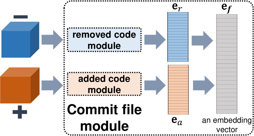
Removed code module. Fig. 7 shows the structure of the removed code module. The input of this module is a three-dimensional matrix, indicating the removed code in a file of a given patch, denoted by , where , , and are the number of hunks, the number of removed code lines for each hunk, and the number of words in each removed code line in the affected file, respectively. This module takes advantage of a commit line module and a 3D convolutional layer (3D-CNN) to construct an embedding vector (denoted by in Fig. 6) representing the removed code in the affected file. We describe the commit line module and the 3D-CNN in the following sections.

a) Commit line module. Each line of removed code in is processed by the commit line module to obtain a list of embedding vectors representing the removed code lines. This module has the same structure as the commit message module, but maintains a code-specific vocabulary and word embedding matrix, as a word may have different meanings in a textual message and in source code.
The obtained commit line vectors are used to construct a new three-dimensional matrix, . represents a sequence of hunks; each hunk has a sequence of removed lines, where each line is now represented as a -dimensional embedding vector () extracted by the commit line module. is then passed to the 3D convolutional neural network (3D-CNN), described below, to construct an embedding vector for the code removed from a file by a given patch.
b) 3D-CNN. The 3D convolutional layer is used to extract features from the code removed from the affected file, as represented by . This layer applies each filter to a window of hunks to build a new feature as follows:
| (5) |
is the sum of element-wise products, is constructed from the -th hunk through the -th hunk in the removed code of the affected file, is the bias value, and is the ReLU activation function. As for the commit message module (see Section III-B), we choose . Fig. 8 shows an example of a 3D convolutional layer that has one filter.
Applying the filter F to all windows of hunks in produces a feature vector:
| (6) |
As in Section III-B, we apply a max pooling operation to to obtain the most important feature. The features selected by max pooling with multiple filters are concatenated unchanged to construct an embedding vector representing information extracted from the removed code changes in the affected file.
Added code module. This module has the same architecture as the removed code module. The changes in the added and removed code are furthermore padded or truncated to have the same number of hunks (), number of lines for each hunk (), and the number of words of each line (), for parallelization. Moreover, both modules also share the same vocabulary and use the same word embedding matrix.
The added code module constructs an embedding vector (denoted by in Fig. 6) representing the added code in a file of a given patch. An embedding vector representing all of the changes made to a given file by a commit is constructed by concatenating the two embedding vectors representing the removed code and added code as follows:
| (7) |
III-C2 Embedding Vector for Commit Code
The embedding vector for all the changes performed by a given patch is constructed as follows:
| (8) |
where simply concatenates two vectors unchanged, denotes the -th file affected by the given commit, is the number of affected files, and denotes the vector constructed by applying the commit file module to the affected file .
III-D Classification Module
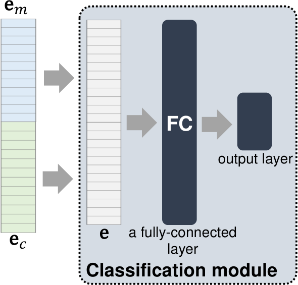
Fig. 9 shows the architecture of the classification module. It takes as input the commit message embedding vector and the commit code embedding vector discussed in Sections III-B and III-C, respectively. The patch is represented by their concatenation as follows:
| (9) |
We then feed the concatenated vector into a fully-connected (FC) layer, which outputs a vector as follows:
| (10) |
where is a dot product, is a weight matrix associated with the concatenated vector, is the bias value, and is a non-linear activation function. Again, we use ReLU to implement . Note that both and are learned during our model’s training process. Note that both and are learned during our model’s training process.
Finally, the vector is passed to an output layer, which computes a probability score for a given patch:
| (11) |
where is a weight matrix that is also learned during the training process.
III-E Parameter Learning
During the training process, PatchNet learns the following parameters: the word embedding matrices for commit messages and commit code, the filter matrices and bias of the convolutional layers, and the weights and bias of the fully connected layer and the output layer. The training aims to minimize the following regularized loss function [20]:
| (12) |
where is the probability score from the output layer and contains all the (learnable) parameters as mentioned before.
The term is used to mitigate data overfitting by penalizing large model parameters, thus reducing the model complexity. To further improve the robustness of our model, we also apply the dropout technique [58] on all the convolutional and fully-connected layers in PatchNet.
IV Experiments
We first describe our dataset and how we preprocess it. We then introduce the baselines and evaluation metrics. Finally, we present our research questions and results.
IV-A Dataset
We take our data from the patches that have been committed to mainline Linux kernel22 2 git://git.kernel.org/pub/scm/linux/kernel/git/torvalds/linux.git v3.0, released in July 2011, through v4.12, released in July 2017. We additionally collect information from the stable kernels33 3 git://git.kernel.org/pub/scm/linux/kernel/git/stable/linux.git that had been released as of October 2017 building on Linux kernels v3.0 through v4.13. We consider a mainline commit to be stable if it is duplicated in at least one stable version. To increase the set of commits that can be used for training, we furthermore include in the training set of stable patches other Linux kernel commits that are expected by convention to be bug-fixing patches. Indeed, a Linux kernel release is created by first collecting a set of commits for the coming release into a preliminary release called a “release candidate”, named rc1, that may include new features and bug fixes. This is followed by a succession of further release candidates, named rc2 onwards, that should include only bug fixes. We thus also include the commits added for release candidates rc2 onwards in our set of stable patches.
We refer to patches that are propagated to stable kernels or are found in later release candidates as stable patches and patches that are not propagated to stable kernels or found in later release candidates as non-stable patches. To avoid biasing the learning process towards either stable or non stable patches, we construct our training datasets such that the number of patches in each category is roughly balanced. While this situation does not reflect the number of stable and non-stable patches that confront a stable kernel maintainer each day, it allows effective training and interpretation of the experimental results.
IV-A1 Identifying Stable Patches
The main challenge in constructing the datasets is to determine which mainline patches have been propagated to stable kernels. Indeed, there is no required link information connecting the two. Many stable patches explicitly mention the corresponding mainline commit in the commit message, which we refer to as a back link. For others, we rely on the author name and the subject line. Subject lines typically contain information about both the change made and the name of the file or directory in which the change is made, and should be unique. We first collect from the patches in the stable kernels a list of back links and a list of pairs of author name and subject line. A commit from the mainline whose commit id is mentioned in a back link or whose author name and subject line are the same as one found in a patch to a stable kernel is considered to be a stable patch.
IV-A2 Collecting the Dataset
We collect our dataset from the mainline Linux kernel. In order to focus on patches that are challenging for stable maintainers to classify, we drop in advance all patches that do not meet the stable-kernel size guidelines,44 4 https://www.kernel.org/doc/html/v4.15/process/stable-kernel-rules.html i.e., those that exceed 100 code lines, including both changed lines and context as reported by diff. We subsequently keep all identified stable patches for our dataset and select an equal number of non-stable patches. Whenever possible, we select non-stable patches that have a similar number of changed lines as the stable patches, again to create a dataset that reflects the cases that cannot be excluded by size alone and thus are challenging for stable kernel maintainers. These patches are then subject to a preprocessing step that is detailed in the next section. We do not use the dataset studied by Tian et al. [63], because it is seven years old and unclean, including labeling as bug-fixing patches the results of tools that may report coding style issues or faults whose impact is not visible in practice.
Our dataset comes from Linux kernel mainline versions 3.0 (July 2011) through 4.12 (July 2017). There were 424,380 commits during that period. We consider only those commits that are not merge commits, that modify a file as opposed to only adding or removing files, and that affect at least one .c or .h file. This leaves 346,570 commits (82%). Of these 346,570 commits, 79,319 (23%) are not considered because they contain more than 100 changed lines, leaving 267,251 commits. Of these,to have a balanced training dataset, we pick the 42,408 stable patches for which the preprocessing step is successful (see below,) and 39,995 non-stable patches, i.e., 82,403 patches in all. In RQ4, we consider the full set of Linux kernel patches in versions v3.0-v4.12 that are accepted by our preprocessing step.
IV-B Patch Preprocessing
Our approach applies some preprocessing steps to the patches before they are given to PatchNet.
IV-B1 Preprocessing of Commit Messages
Our approach applies various standard natural language techniques to the commit messages, such as stop word elimination and stemming [65, 6], to reduce message length and eliminate irrelevant information. Subsequently, we pad or truncate all commit messages to the same size, specifically 512 words, covering the complete commit message for all patches, for parallelism. Because we are interested in cases that are challenging for the stable kernel maintainer, we drop tags such as Cc: stable and Fixes, whose goal is to indicate that a given patch is a stable or a bug fixing patch. We also drop tags indicating who has approved the patch, as the set of developers and their work profiles can change in the future.
IV-B2 Preprocessing of Code Changes
Diff code elements, as illustrated in Fig. 1(a), may have many shapes and sizes, from a single word to multiple lines spread out over multiple hunks. To describe changes in terms of meaningful syntactic units and to provide context for very small changes, we collect differences at the granularity of atomic statements. These may be, e.g., simple assignment statements, return statements, if headers, etc. For example, in the patch illustrated in Fig. 1(a), the only change is to replace 1 on line 22 by err on line 23. Nevertheless, we represent the change as a change in the complete return statement, i.e., return 1; that is transformed into return err;. We also distinguish changes in error checking code (code to detect whether an error has occurred, e.g., line 21 in Fig. 1(a)) and in error handling code (code to clean up after an error has occurred, e.g., lines 22 and 23 in Fig. 1(a)) from changes in other code, which we refer to as normal code. Error handling code is considered to be any code that is in a conditional with only one branch, where the conditional ends in a return with an argument other than 0 (0 is typically the success indicator) or a goto, as well as any code following a label that ends in a return with an argument other than 0 or a goto. Error checking code is considered to be the header of a conditional that matches the former pattern. These criteria are not completely reliable, as such code can sometimes represent the success case rather than a failure case, but they are typically followed and are actively promoted by Linux kernel developers. Error checking code and error handling code are very common in the Linux kernel, which must be robust, and they are disjoint in structure and purpose from the implementation of the main functionality.
For a given commit, the first step is to extract the names of the affected files and to extract the state of those files before and after the commit. Analogous to the stemming and stop word elimination performed at the commit message level, for each before and after file instance, we remove comments and the contents of strings, as changes in comments and within strings are not likely to be needed in stable kernels. For a given pair of before and after files, we then compute the difference using the command “git diff -U0 old new”, giving the changed lines with no lines of surrounding context. For each “–” or “+” line in the diff output, we then collect a record indicating the sign (“–” or “+”), the category (error-handling code, etc.), the hunk number, the line number in the old or new version, respectively, and the starting and ending columns of the non-space changes on the line. We furthermore keep the names of called functions, when these are not defined in the same file and are used at least 5 times, but drop other identifiers, i.e. field names and variable names, as these may be too diverse to allow effective learning and unnecessarily slow down the training time. Indeed, adding just the frequently used function names increases the code vocabulary size from 43 to 3,616 unique tokens, which increases the training time.
To extract changes at the level of atomic statements, rather than the individual lines obtained by diff, we parse each file as it exists before and after the change and keep the atomic statements that intersect with a changed line observed by diff. For this, we use the parser of the C program transformation system Coccinelle [55], which uses heuristics to parse around compiler directives and macros [54]. This makes it possible to reason about patches in terms of the way they appear to the user, without macro expansion, but comes with some cost, as some patches must be discarded because the parsing heuristics are not sufficient to parse all of the code affected by the changed lines.
By following the above-mentioned steps, we collect the files affected by a given patch. For each removed or added code line of an affected file, denoted by “–” and “+”, we collect the corresponding hunk number and line number. Each word in a line is a pair of the associated token and the annotation indicating whether the word occurs on a line of as error-checking code, error-handling code, or normal code. This information is used to build the two three-dimensional matrices representing the removed code and the added code for the affected file (see Fig. 6).
IV-C Baselines
We compare PatchNet with several baselines:
- •
Keyword: As a simple but frequently used heuristic [63], we select all commits in which the commit message includes “bug”, “fix”, or “bug-fix” after conversion of all words to lowercase and stemming. While not all bug fixes are relevant for stable kernels, as some bugs may have very low impact or the fix may be too large or complex to be considered clearly correct, the problem of identifying bug fixes is close enough to that of recognizing stable patches to make comparison with our model valuable.
- •
LPU+SVM: This method was proposed by Tian et al. [63] and combine Learning from Positive and Unlabeled Examples (LPU) [27, 42, 45] and Support Vector Machine (SVM) [10, 12], to build a classification model for automatically identifying bug fixing patches. The set of code features considered was manually selected. In Tian et al.’s work, stable kernels were considered as a source of bug-fixing patches in the training and testing data.
- •
LS-CNN: Huo et al. [24] combined LSTM [23] and CNN [39] to localize potential buggy source files based on bug report information. They used CNN to learn a representation of the bug report and a combination of LSTM and CNN to learn the structure of the code. To assess the ability of LS-CNN to classify patches as stable, for a given patch, we give the commit message and the code changes (i.e., the result of concatenating the lines changed in the various files and hunks) as input to LS-CNN in place of the bug report and the potential buggy source file, respectively. To make a fair comparison, the CNN used to learn the representation of the commit message in LS-CNN has the same architecture (i.e., number of convolutional layer, filter size, activation function, etc.) as the CNN used to learn the representation of the commit message in PatchNet.
- •
Feed-forward fully connected neural network (F-NN): Inspired by PatchNet and the work of Tian et al. on LPU+SVM, a Linux stable kernel maintainer, Sasha Levin, has developed an approach to identifying stable patches [43] based on a feed-forward fully connected neural network [4, 15] and a set of manually selected features, including frequent commit message words, author names, and some code metrics. Levin actively uses this approach in his work on the Linux kernel.
For LPU-SVM and LS-CNN, we used the same parameters and settings as described in the respective papers. For F-NN, we asked Levin to train the tool on our training data and test it with our testing data. We use 50% as the cut off for considering a patch as stable for PatchNet and all baselines.
IV-D Experimental Settings
PatchNet has several hyperparameters (i.e., the sizes of the filters, the number of convolutional filters, the size of the fully-connected layer, etc.) that we instantiate them in the following paragraph.
For the sizes of the filters described in Section III, we choose , making the associated windows analogous to a 1-gram or 2-gram as used in natural language processing [28, 7]. Using 2-grams allows our approach to take into account the temporal ordering of words, going beyond the bag of words used by Tian et al. [63]. The number of convolutional filters is set to 64. The size of the fully-connected layer described in Section III-D is set to 100. The dimensions of the word vectors in commit message and code changes are set to 50. PatchNet is trained using Adam [32] with shuffled mini-batches. The batch size is set to 32. We train PatchNet for 50 epochs and apply the early stopping strategy [56, 9], i.e., we stop the training if there has been no update to the loss value (see Equation 12) for the last 5 epochs. All these hyperparameter values are widely used in the deep learning community [57, 25, 24, 22]. For parallelization, the number of changed files, the number of hunks for each file, the number of lines for each hunk, the number of words of each removed or added code are set to 5, 8, 10, and 120, respectively.
In our experiments, we run PatchNet on Ubuntu 18.04.3 LTS, 64 bit, with a Tesla P100-SXM2-16GB5 GPU.55 5 https://www.nvidia.com/en-us/data-center/tesla-p100/ Training takes around 20 hours and testing less than 30 minutes to process 16,481 patches (one of the five folds presented in Section IV-F). Note that training only needs to be done periodically (e.g., weekly/monthly) and the trained model can be used to label many patches. In our experiments, on average, the trained PatchNet can assign a label to a single patch in 0.11 seconds.
IV-E Evaluation Metrics
To evaluate the effectiveness of a stable patch identification model, we employ the following metrics:
- •
Accuracy: Proportion of stable and non-stable patches that are correctly classified.
- •
Precision: Proportion of patches that are correctly classified as stable.
- •
Recall: Proportion of stable patches that are correctly classified.
- •
F1 score: Harmonic mean between precision and recall
- •
AUC: Area under the Receiver Operating Characteristic curve, measuring if the stable patches tend to have higher predicted probabilities (to be stable) than non-stable ones.
IV-F Research Questions and Results
Our study seeks to answer several research questions (RQs):
RQ1: Do the properties of stable and non-stable patches change over time? A common strategy for evaluating machine learning algorithms is -fold cross-validation [33], in which a dataset is randomly distributed among equal-sized buckets, each of which is considered as test data for a model trained on the remaining buckets. When data elements become available over time, as is the case of Linux kernel patches, this strategy results in testing a model on data that predates some of the data on which the model was trained. Respecting the order of patch submission, however, would limit the amount of testing that can be done, given the fairly small number of stable patches available.
To address this issue, we first assess whether training on future data helps or harms the accuracy of PatchNet. We first sort the patches collected in Section IV-A from earliest to latest based on the date when the patch author submitted the patch to maintainers. Then, we divide the dataset into five mutually exclusive sets by date. Note that the resulting five sets are not perfectly balanced, but they come close, with stable patches making up 45% to 55% of each set. Then, we repeat the following process five times: take one set as a testing set and use the remaining four sets for training. Testing on the first set shows the impact of training only on future data. Testing on the fifth set shows the impact of training only on past data. The other testing sets use models trained on a mixture of past and future data.
Table I shows the results of PatchNet on the different test sets. The standard deviations are quite small (i.e., at most 0.013), hence there is no difference between training on past or future data. Our dataset starts with Linux v3.0, which was released in 2011, twenty years after the start of work on the Linux kernel. The lack of impact due to training on past or future data suggests that in such a mature code base the properties that make a patch relevant for stable kernels are fairly constant over time. This property is indeed beneficial, because it means that our approach can be used to identify stable commits that have been missed in older versions. In the subsequent research questions, we thus retain the same five test and training sets.
| Accuracy | Precision | Recall | F1 | AUC | |
| Set=1 | 0.852 | 0.841 | 0.886 | 0.863 | 0.850 |
| Set=2 | 0.860 | 0.833 | 0.909 | 0.869 | 0.859 |
| Set=3 | 0.866 | 0.833 | 0.910 | 0.870 | 0.867 |
| Set=4 | 0.864 | 0.828 | 0.912 | 0.868 | 0.864 |
| Set=5 | 0.869 | 0.860 | 0.917 | 0.887 | 0.862 |
| Std. | 0.007 | 0.013 | 0.012 | 0.009 | 0.007 |
RQ2: How effective is PatchNet compared to other state-of-the-art stable patch identification models? To answer this RQ, we use the five test sets of the dataset described in RQ1. Of these, we take one test set as the testing data and regard the remaining patches as the training data. We repeat this five times, and then average the results to get the aggregated accuracy, precision, recall, F1, and AUC scores. Table II shows the results for PatchNet and the other baselines. PatchNet achieves average accuracy, precision, recall, F1 score, and AUC of 0.862, 0.839, 0.907, 0.871, and 0.860, respectively. Compared to the best performing baseline, F-NN, these constitute improvements of 6.55%, 0.12%, 16.13%, 7.80%, and 6.30%, respectively. PatchNet thus achieves about the same precision as F-NN, but a significant improvement in terms of recall. This is achieved without the feature engineering required for the F-NN approach, but rather by automatically learning the weight of the filters via our hierarchical deep learning-based architecture.
We also employ Scott-Knott ESD ranking [61] to statistically compare the performance of PatchNet and the four considered approaches (i.e., PatchNet, F-NN, LS-CNN, and LPU-SVM). The results show that PatchNet consistently appears in the top Scott-Knott ESD rank in terms of accuracy, precision, recall, F1 score, and AUC. The ranks of the four considered approaches are furthermore consistent (i.e., PatchNet F-NN LS-CNN LPU-SVM) except for recall (i.e., PatchNet LS-CNN F-NN LPU-SVM).
| Accuracy | Precision | Recall | F1 | AUC | |
|---|---|---|---|---|---|
| Keyword | 0.626 | 0.683 | 0.515 | 0.587 | 0.630 |
| LPU+SVM | 0.731 | 0.751 | 0.716 | 0.733 | 0.731 |
| LS-CNN | 0.765 | 0.766 | 0.785 | 0.775 | 0.765 |
| F-NN | 0.809 | 0.838 | 0.781 | 0.808 | 0.809 |
| PatchNet | 0.862 | 0.839 | 0.907 | 0.871 | 0.860 |
Fig. 10 compares the precision-recall curves for PatchNet and the baselines. For most values on the curve, PatchNet obtains the highest recall for a given precision and the highest precision for a given recall. For example, for a low false positive rate of 5 percent (precision of 0.95), PatchNet achieves a recall of 0.786 which is 14.9% higher than that of the best performing baseline. Likewise, for a low false negative rate of 5 percent (recall of 0.95), PatchNet achieves a precision of 0.603 which is 41.2% higher than that of the best performing baseline. In addition, considering the sweet spots where both precision and recall are high (larger than 0.8), PatchNet can achieve an F1 score of up to 0.886 which is 10.6% higher than that of the best performing baseline.
Fig. 11 shows Venn diagrams indicating the number of patches that PatchNet and each of the baselines correctly recognize as stable. The top diagram compares the Keyword approach to the two approaches, PatchNet and LS-CNN, that automatically learn the relevant features. While there are over 20K patches that all three approaches classify as stable, there are another 11K that are found by both learning-based approaches, showing the advantage of learning-based approach. As compared to Keyword and LS-CNN, there are almost 7,000 patches that are only recognized by PatchNet, while this is the case for fewer than 2,000 patches for LS-CNN, showing the value of an approach that takes the properties of code changes into account.
The bottom diagram then compares PatchNet to the two approaches, LPU+SVM and F-NN, in which the code features are handcrafted. While all three approaches correctly recognize over 27K patches as stable, there are again 3x more patches that only PatchNet correctly detects as stable than there are that only each of the other two approaches recognizes as stable. Examples of PatchNet true positives not found by the other baselines include 5567e989198b66 6 git://git.kernel.org/pub/scm/linux/kernel/git/torvalds/linux.git and 2e31b4cb895a. Examples of PatchNet false negatives found by at least one other baseline include 03f219041fdb and 56199016e867.
All of the above measures of precision and recall assume that the set of patches found in the tested Linux kernel versions is the correct one. Our motivation, however, is that bug fixing patches that should be propagated to the Linux kernel stable versions are being overlooked by the existing manual labeling process. Showing that PatchNet improves on the existing manual process requires collecting a dataset of patches that have not been propagated to stable kernels, but should have been. Collecting such a dataset, however, requires substantial Linux kernel expertise, which it is not feasible to harness at a large scale. We have nevertheless been able to carry out two experiments in this direction. First, we randomly selected 200 patches predicted as stable patches by PatchNet, but that were not marked as stable in our dataset. We sent the 200 patches to Sasha Levin (a Linux stable-kernel maintainer and the developer of F-NN) to label. Among the 200 patches, Levin labeled 61 patches (i.e., 30.5%) as stable, highlighting that our approach can find many additional stable patches that were not identified by the existing manual process. Note that these patches predated Levin’s used of F-NN on the Linux kernel. Second, we looked at commits that have no Cc stable tag that Sasha Levin selected with the aid of F-NN for the Linux 4.14 stable tree. These commits postdate all of the commits in our dataset. There are over 1,800 of them, showing the false negatives in the existing manual process and the need for automated support. PatchNet detects 91% of them as stable. The relationship between the results of F-NN and PatchNet is similar to that shown in Fig. 11 for patches in our original dataset and confirms that PatchNet can find stable patches that were not identified by the existing manual process.
RQ3: Does PatchNet benefit from considering both the commit message and the code changes, and do function names help identify stable patches? To answer this RQ, we conduct an ablation test [34, 46] by ignoring the commit message, the code changes, or the function names in the code changes in a given patch one-at-a-time and evaluating the performance. We create three variants of PatchNet: PatchNet-C, PatchNet-M, and PatchNet-NN. PatchNet-C uses only code change information while PatchNet-M uses only commit message information. PatchNet-NN uses both code change and commit message information, but ignores the function names in the code changes. We again use the five copies of the dataset described in RQ1 and compute the various evaluation metrics.
Table III shows that the performance of PatchNet degrades if we ignore any one of the considered types of information. Accuracy, precision, recall, F1 score, and AUC drop by 19.39%, 15.41%, 21.26%, 18.34%, and 16.06% respectively if we ignore commit messages. They drop by 16.96%, 14.62%, 16.58%, 14.76%, and 14.21% respectively if we ignore code changes. And they drop by 11.08%, 12.62%, 16.43%, 13.86%, and 11.98% respectively if we ignore function names. Thus, each kind of information contributes to PatchNet’s performance. Additionally, the drops are greatest if we ignore commit messages, indicating that they are slightly more important than the other two to PatchNet’s performance.
| Accuracy | Precision | Recall | F1 | AUC | |
|---|---|---|---|---|---|
| PatchNet-C | 0.722 | 0.727 | 0.748 | 0.736 | 0.741 |
| PatchNet-M | 0.737 | 0.732 | 0.778 | 0.759 | 0.753 |
| PatchNet-NN | 0.776 | 0.745 | 0.779 | 0.765 | 0.768 |
| PatchNet | 0.862 | 0.839 | 0.907 | 0.871 | 0.860 |
RQ4: What are the results of PatchNet on the complete set of Linux kernel patches? For RQ1, we use a dataset collected such that the number of stable and non-stable patches is roughly balanced. Among the 267,251 patches that meet the selection criteria, we picked 42,408 stable patches and 39,995 non-stable patches to build our dataset. To investigate the results of PatchNet on the complete set of patches from Linux v3.0-v4.12 having at most 100 lines (and accepted by our preprocessor), we randomly divide the remaining 184,481 non-stable patches into five sets and merge each of them with each of the five test sets described in RQ1. After this process, we have a new collection of five test sets. In each test set, there are around 8.4K stable patches and 44.8K non-stable patches. For each new test set, we use the corresponding model trained for RQ1. We repeat this five times, and then average the results to get the aggregated AUC score. PatchNet achieves an average AUC of 0.808. Since the new five test sets are highly imbalanced (only 15.79% patches are stable patches), we omit the other metrics (i.e., accuracy, precision, recall, and F1) [53, 60, 49]. We also trained PatchNet on a whole training dataset (i.e., 42,408 stable patches and 39,995 non-stable patches) and evaluated it on 184,481 non-stable patches. We find that PatchNet can correctly label them as non-stable 81.32% of the time.
We also check the effectiveness of PatchNet on patches that have more than 100 lines of code (i.e., long patches). As mentioned earlier, we omit those patches from our training dataset as they do not meet the selection criteria of Linux kernel. We collect 52,415 long patches from July 2011 to July 2017. Among them, there are 3,376 long stable patches and 49,039 long non-stable patches. 21.33% of these patches contain the “Cc: stable” tag. The others may have been manually selected for stable versions despite not having a tag or may come from the release candidates. We again train PatchNet on the whole training dataset and evaluate the effectiveness of PatchNet on the 52,415 long patches. PatchNet achieves an AUC score of 0.805. Again we only use AUC as this dataset is highly imbalanced [53, 60, 49].
Finally, we also check whether there is a difference of performance in classifying patches containing a “Cc: stable” tag and patches that do not containing a “Cc: stable” tag. Among the 42,408 stable patches, there are 15,410 stable patches with a stable tag and 26,998 stable patches with no stable tag. The latter may again have been manually selected for stable versions despite not having a tag or may come from the release candidates. For each test set described in RQ1, we split the stable patches into two groups: tagged stable patches and non-tagged stable patches. We run PatchNet on the stable patches of each test set to predict the stable patches and sum the results of predicting the stable patches. Among 15,410 tagged stable patches, PatchNet predicts 14,578 patches as stable patches (i.e., 94.60%). Among the 26,998 non-tagged stable patches, PatchNet predicts 23,466 patches as stable patches (i.e., 86.92%). We find that PatchNet is more successful at recognizing tagged patches, even when it does not have access to information about the “Cc: stable” tag.
V Qualitative Analysis and Discussion
In this section, we analyze some of the results obtained in Section IV-F, considering in detail a patch where PatchNet performs well and another where it performs poorly.
V-A Successful Case
We first present a patch that PatchNet can predict as a stable patch, intending to show an advantage of our model.
Figure 12 shows a patch propagated to stable kernels. The commit message is on line 5 and the code changes are on lines 16-59. The code changes include one changed file, five hunks, 12 removed lines, and 25 added lines. PatchNet is able to predict the patch in Figure 12 as stable patch. We see that the commit message of this patch is quite short and does not contain keywords such as “bug” or “fix”. To recognize the patch as a stable patch, the stable kernel maintainer has to study the code changes to understand the impact of the changes in the kernel code. In the code changes, the four variables (i.e, left, right, top, and bottom) are defined and used across the multiple hunks in the changed file (i.e., vmwgfx_kms.c). We also see the difference between removed lines and added lines when the author committed his code. By representing the removed code and the added code as two three-dimensional matrices (each dimension represents the number of hunks, the number of removed or added code lines, and the number of words in each removed or added code line), PatchNet uses the removed code module and the added code module to construct the embedding vector of the removed code and added code, respectively (see Section III-C). The two embedding vectors are then concatenated to represent the code change information. By doing this process, the distinction between removed lines and added lines is preserved. PatchNet automatically learns from this rich representation by updating its parameters during the training process (see Section IV-D) to build a model that can predict whether a patch is stable.
On the other hand, we find that none of the other baselines are able to classify the patch in Figure 12 as a stable patch. Keyword is a heuristic approach that only looks at whether the content of a commit message includes “bug” or “fix”. LS-CNN concatenates the removed lines and added lines in the multiple hunks without preserving the code changes information. LPU+SVM and F-NN define a set of features for the code changes (i.e., the number of removed code lines, the number of added code lines, the number of hunks in a commit, etc.). The manual creation of code changes features may overlook features that are important to identify stable patches, making LPU+SVM and F-NN unable to classify the patch in Figure 12 as a stable patch.
V-B Unsuccessful Case
Next, we present a patch that PatchNet fails to classify correctly as a stable patch. This example serves to provide an understanding of cases in which PatchNet may not perform well.
Figure 13 shows a stable patch that was not recognized by PatchNet. Its commit message does not contain any keywords (i.e., “bug” or “fix”) that suggest whether the patch is a stable patch. The code changes only include one removed line and the removed line contains only three words: vma, vm_flags, and VM_IO. As there is very little information in both the commit message and the code changes, PatchNet is unable to predict the patch in Figure 13 as a stable patch. We find that the other baselines (i.e, keywords, LS-CNN, and LPU+SVM), except F-NN, also fail to classify the patch as a stable patch. F-NN considers not only the commit message and the code changes of the given patch, but also information such as author name, reviewer information, file names, etc. This suggests that when the information of the commit message and the code changes is limited, an approach that takes advantage of other information in a given patch may perform better than PatchNet.
VI Threats to Validity
Internal validity. Threats to internal validity relate to errors in our experiments and experimenter bias. We have double checked our code and data, but errors may remain. In the baseline approach by Tian et al. [63], commits were labeled by an author with expertise in Linux kernel code, which may introduce author bias. In this work, none of the authors label the commits.
External validity. Threats to external validity relate to the generalizability of our approach. We have evaluated our approach on more than 80,000 patches. We believe this is a good number of patches. Still, the results may differ if we consider other sets of Linux kernel patches. Similar to the evaluation of Tian et al. [63], we only investigated Linux kernel patches, although PatchNet can be applied to patches of other systems, if labels are available. In the future, we would like to consider more projects. Still, we note that the Linux kernel represents one of the largest open source projects, with over 16 million lines of C code, and that different kernel subsystems have different developers and very different purposes, resulting in a wide variety of code.
Construct validity. Threats to construct validity relate to the suitability of our evaluation metrics. We use standard metrics commonly used to evaluate classifier performance. Thus, we believe there is little threat to construct validity.
VII Related Work
Researchers have applied deep learning techniques to solve software engineering problems, including code clone detection [68, 44, 8], software traceability link recovery [17], bug localization [25, 36], defect detection [70, 66], automated program repair [18], and API learning [16]. However, we did not find any research that applied deep learning techniques to learn semantic representations of patches for similar tasks such as stable patch identification, patch classification, etc. Here, we briefly describe the most closely related work besides the baselines described in Section IV-C.
Sequence-to-sequence learning. Gu et al. adopted a neural language model named a Recursive Neural Network (RNN) [19, 50] encoder-decoder to generate API usage sequences, i.e., a sequence of method names, for a given natural language query [16]. Gupta et al. proposed DeepFix to automatically fix syntax errors in C code [18]. DeepFix leverages a multi-layered sequence-to-sequence neural network with attention [51], to process the input code and a decoder RNN with attention that generates the output fixed code. The above studies focus on learning sequence-to-sequence mappings and thus consider a different task than the one considered in our work.
Learning code representation. CCLearner [44] learns a deep neural network classifier from clone pairs and non clone pairs to detect clones. To represent code, it extracts features based on different categories (reserved words, operators, etc.) of tokens in source code. White et al. presented another deep learning-based clone detector [68]. Their tool first uses RNN to map program tokens to continuous-valued vectors, and then uses RNN to combine the vectors with extracted syntactic features to train a classifier. Wang et al. used a deep belief network (DBN) [21] to predict defective code [66]. The DBN learns a semantic representation (in the form of a continuous-valued vector) of each source code file from token vectors extracted from programs’ ASTs. Lam et al. combined deep learning with information retrieval to localize buggy files based on bug reports [36]. Bui and Jiang proposed a deep learning based approach to automatically learn cross-language representations for various kinds of structural code elements (i.e., expressions, statements, and methods) for program translation [8]. Different from the above studies, we design a novel deep learning architecture that focuses on code changes, taking into account their hierarchical and structural properties.
Learning of both code and text representations. Huo and Li proposed a model, LS-CNN, for classifying if a source code file is related to a bug report (i.e., the source code file needs to be fixed to resolve the bug report) [24]. LS-CNN is the first code representation learning method that combines CNN and LSTM (a specific type of RNN) to extract semantic representations of both code (in their case: a source code file) and text (in their case: a bug report). Similar to LS-CNN, PatchNet also learns semantic representations of both code and text. However, different from LS-CNN, PatchNet includes a new representation learning architecture for commit code comprising the representations of removed code and added code of each affected file in a given patch. The representation of removed code and added code is able to capture the sequential nature of the source code inside a code change, and it is learned following a CNN-3D architecture [26] instead of LSTM. Our results in Section IV show that PatchNet can achieve an 11.24% improvement in terms of F1 over the LS-CNN model.
VIII Conclusion
In this paper, we propose PatchNet, a hierarchical deep learning-based model for identifying stable patches in the Linux kernel. For each patch, our model constructs embedding vectors from the commit message and the set of code changes. The embedding vectors are concatenated and then used to compute a prediction score for the patch. Different from existing deep learning techniques working on the source code [68, 66, 24, 44, 17, 36, 16], our hierarchical deep learning-based architecture takes into account the structure of code changes (i.e., files, hunks, lines) and the sequential nature of source code (by considering each line of code as a sequence of words) to predict stable patches in the Linux kernel.
We have extensively evaluated PatchNet on a new dataset containing 82,403 recent Linux kernel patches. On this dataset, PatchNet outperforms four baselines including two also based on deep-learning. In particular, for a wide range of values in the precision-recall curve, PatchNet obtains the highest recall for a given precision, as well as the highest precision for a given recall. For example, PatchNet achieves a 14.9% higher recall (0.786) at a high precision level (0.950) and a 41.2% higher precision (0.603) at a high recall level (0.950) compared to the best-performing baseline.
In future work, we want to investigate ways to improve our approach further, e.g., by incorporating additional data such as more kinds of names and type information. Another issue is to identify the stable versions to which a patch should be applied. We plan to investigate whether machine learning can help with this issue. It would also be interesting to apply our approach that learns patch embeddings to other related problems, e.g. identification of valid/invalid patches in automated program repair [69], assignment of patches to developers for code review [62, 71], etc.
Dataset and Code. The dataset and code for PatchNet are available at https://github.com/hvdthong/PatchNetTool. A video demonstration of PatchNet is available at https://goo.gl/CZjG6X.
Acknowledgement. This research was supported by the Singapore National Research Foundation (Award number: NRF2016-NRF-ANR003) and the ANR ITrans project.
References
- [1] G. A. Anastassiou, “Univariate hyperbolic tangent neural network approximation,” Mathematical and Computer Modelling, vol. 53, no. 5-6, pp. 1111–1132, 2011.
- [2] M. Anthimopoulos, S. Christodoulidis, L. Ebner, A. Christe, and S. Mougiakakou, “Lung pattern classification for interstitial lung diseases using a deep convolutional neural network,” IEEE transactions on medical imaging, vol. 35, no. 5, pp. 1207–1216, 2016.
- [3] S. Arora, N. Cohen, and E. Hazan, “On the optimization of deep networks: Implicit acceleration by overparameterization,” in 35th International Conference on Machine Learning (ICML), 2018, pp. 244–253.
- [4] C. M. Bishop et al., Neural networks for pattern recognition. Oxford university press, 1995.
- [5] L. Bottou, “Large-scale machine learning with stochastic gradient descent,” in Proceedings of the 19th International Conference on Computational Statistics (COMPSTAT). Springer, 2010, pp. 177–186.
- [6] T. Brants, “Natural language processing in information retrieval.” in CLIN, 2003.
- [7] P. F. Brown, P. V. Desouza, R. L. Mercer, V. J. D. Pietra, and J. C. Lai, “Class-based n-gram models of natural language,” Computational Linguistics, vol. 18, no. 4, pp. 467–479, 1992.
- [8] N. D. Bui and L. Jiang, “Hierarchical learning of cross-language mappings through distributed vector representations for code,” in Proceedings of the 40th International Conference on Software Engineering: New Ideas and Emerging Results. ACM, 2018, pp. 33–36.
- [9] R. Caruana, S. Lawrence, and C. L. Giles, “Overfitting in neural nets: Backpropagation, conjugate gradient, and early stopping,” in Advances in neural information processing systems, 2001, pp. 402–408.
- [10] G. Cauwenberghs and T. Poggio, “Incremental and decremental support vector machine learning,” in Advances in neural information processing systems, 2001, pp. 409–415.
- [11] R. Collobert, J. Weston, L. Bottou, M. Karlen, K. Kavukcuoglu, and P. Kuksa, “Natural language processing (almost) from scratch,” Journal of Machine Learning Research, vol. 12, no. Aug, pp. 2493–2537, 2011.
- [12] N. Cristianini, J. Shawe-Taylor et al., An introduction to support vector machines and other kernel-based learning methods. Cambridge university press, 2000.
- [13] G. E. Dahl, T. N. Sainath, and G. E. Hinton, “Improving deep neural networks for LVCSR using rectified linear units and dropout,” in Proceedings of IEEE International Conference on Acoustics, Speech and Signal Processing (ICASSP). IEEE, 2013, pp. 8609–8613.
- [14] “Everything you ever wanted to know about Linux-stable releases,” https://www.kernel.org/doc/html/v4.15/process/stable-kernel-rules.html.
- [15] I. Goodfellow, Y. Bengio, A. Courville, and Y. Bengio, Deep learning. MIT press Cambridge, 2016, vol. 1.
- [16] X. Gu, H. Zhang, D. Zhang, and S. Kim, “Deep API learning,” in FSE. ACM, 2016, pp. 631–642.
- [17] J. Guo, J. Cheng, and J. Cleland-Huang, “Semantically enhanced software traceability using deep learning techniques,” in ICSE. IEEE Press, 2017, pp. 3–14.
- [18] R. Gupta, S. Pal, A. Kanade, and S. Shevade, “Deepfix: Fixing common C language errors by deep learning.” in AAAI, 2017, pp. 1345–1351.
- [19] M. T. Hagan, H. B. Demuth, M. H. Beale, and O. De Jesús, Neural network design. Pws Pub. Boston, 1996, vol. 20.
- [20] S. S. Haykin, Kalman filtering and neural networks. Wiley Online Library, 2001.
- [21] G. E. Hinton, “Deep belief networks,” Scholarpedia, vol. 4, no. 5, p. 5947, 2009.
- [22] G. E. Hinton, N. Srivastava, A. Krizhevsky, I. Sutskever, and R. R. Salakhutdinov, “Improving neural networks by preventing co-adaptation of feature detectors,” arXiv preprint arXiv:1207.0580, 2012.
- [23] S. Hochreiter and J. Schmidhuber, “Long short-term memory,” Neural Computation, vol. 9, no. 8, pp. 1735–1780, 1997.
- [24] X. Huo and M. Li, “Enhancing the unified features to locate buggy files by exploiting the sequential nature of source code,” in IJCAI. AAAI Press, 2017, pp. 1909–1915.
- [25] X. Huo, M. Li, and Z.-H. Zhou, “Learning unified features from natural and programming languages for locating buggy source code.” in IJCAI, 2016, pp. 1606–1612.
- [26] S. Ji, W. Xu, M. Yang, and K. Yu, “3D convolutional neural networks for human action recognition,” IEEE Transactions on Pattern Analysis and Machine Intelligence, vol. 35, no. 1, pp. 221–231, 2013.
- [27] T. Joachims, “SVM-Light support vector machine,” SVM-Light Support Vector Machine http://svmlight. joachims. org/, University of Dortmund, vol. 19, no. 4, 1999.
- [28] D. Jurafsky and J. H. Martin, Speech and language processing. Pearson London, 2014, vol. 3.
- [29] N. Kalchbrenner, E. Grefenstette, and P. Blunsom, “A convolutional neural network for modelling sentences,” in Proceedings of the 52nd Annual Meeting of the Association for Computational Linguistics (ACL). Baltimore, Maryland: Association for Computational Linguistics, June 2014, pp. 655–665. [Online]. Available: http://www.aclweb.org/anthology/P14-1062
- [30] A. Karpathy, G. Toderici, S. Shetty, T. Leung, R. Sukthankar, and L. Fei-Fei, “Large-scale video classification with convolutional neural networks,” in Proceedings of the IEEE conference on Computer Vision and Pattern Recognition, 2014, pp. 1725–1732.
- [31] Y. Kim, “Convolutional neural networks for sentence classification,” in Proceedings of the 2014 Conference on Empirical Methods in Natural Language Processing (EMNLP), 2014, pp. 1746–1751. [Online]. Available: http://aclweb.org/anthology/D/D14/D14-1181.pdf
- [32] D. P. Kingma and J. Ba, “Adam: A method for stochastic optimization,” in Proceedings of 3rd International Conference on Learning Representations (ICLR), 2015.
- [33] R. Kohavi, “A study of cross-validation and bootstrap for accuracy estimation and model selection,” in IJCAI, vol. 14, no. 2. Montreal, Canada, 1995, pp. 1137–1145.
- [34] B. Korbar, A. M. Olofson, A. P. Miraflor, C. M. Nicka, M. A. Suriawinata, L. Torresani, A. A. Suriawinata, and S. Hassanpour, “Deep learning for classification of colorectal polyps on whole-slide images,” Journal of pathology informatics, vol. 8, 2017.
- [35] A. Krizhevsky, I. Sutskever, and G. E. Hinton, “Imagenet classification with deep convolutional neural networks,” in Advances in neural information processing systems, 2012, pp. 1097–1105.
- [36] A. N. Lam, A. T. Nguyen, H. A. Nguyen, and T. N. Nguyen, “Bug localization with combination of deep learning and information retrieval,” in Proceedings of the 25th International Conference on Program Comprehension (ICPC), Buenos Aires, Argentina, 2017, pp. 218–229.
- [37] S. Lawrence, C. L. Giles, A. C. Tsoi, and A. D. Back, “Face recognition: A convolutional neural-network approach,” IEEE transactions on neural networks, vol. 8, no. 1, pp. 98–113, 1997.
- [38] Y. LeCun, Y. Bengio, and G. Hinton, “Deep learning,” nature, vol. 521, no. 7553, p. 436, 2015.
- [39] Y. LeCun, L. Bottou, Y. Bengio, and P. Haffner, “Gradient-based learning applied to document recognition,” Proceedings of the IEEE, vol. 86, no. 11, pp. 2278–2324, 1998.
- [40] Y. LeCun, P. Haffner, L. Bottou, and Y. Bengio, “Object recognition with gradient-based learning,” in Shape, contour and grouping in computer vision. Springer, 1999, pp. 319–345.
- [41] G. K. Lee and R. E. Cole, “From a firm-based to a community-based model of knowledge creation: The case of the Linux kernel development,” Organization science, vol. 14, no. 6, pp. 633–649, 2003.
- [42] F. Letouzey, F. Denis, and R. Gilleron, “Learning from positive and unlabeled examples,” in International Conference on Algorithmic Learning Theory (ALT). Springer, 2000, pp. 71–85.
- [43] S. Levin, “Building stable trees with machine learning,” Jun. 2018.
- [44] L. Li, H. Feng, W. Zhuang, N. Meng, and B. Ryder, “CCLearner: A deep learning-based clone detection approach,” in Proceedings of 33rd Software Maintenance and Evolution (ICSME). IEEE, 2017, pp. 249–260.
- [45] B. Liu, Y. Dai, X. Li, W. S. Lee, and P. S. Yu, “Building text classifiers using positive and unlabeled examples,” in Data Mining (ICDM). Third IEEE International Conference on. IEEE, 2003, pp. 179–186.
- [46] J. Liu, W.-C. Chang, Y. Wu, and Y. Yang, “Deep learning for extreme multi-label text classification,” in Proceedings of the 40th International ACM SIGIR Conference on Research and Development in Information Retrieval. ACM, 2017, pp. 115–124.
- [47] R. Love, Linux kernel development. Pearson Education, 2010.
- [48] D. MacKenzie, P. Eggert, and R. Stallman, “Comparing and merging files with gnu diff and patch,” Network Theory Ltd, vol. 4, 2002.
- [49] S. McIntosh and Y. Kamei, “Are fix-inducing changes a moving target? a longitudinal case study of just-in-time defect prediction,” IEEE Transactions on Software Engineering, vol. 44, no. 5, pp. 412–428, 2017.
- [50] T. Mikolov, M. Karafiát, L. Burget, J. Černockỳ, and S. Khudanpur, “Recurrent neural network based language model,” in Eleventh Annual Conference of the International Speech Communication Association, 2010.
- [51] V. Mnih, N. Heess, A. Graves et al., “Recurrent models of visual attention,” in Advances in neural information processing systems, 2014, pp. 2204–2212.
- [52] V. Nair and G. E. Hinton, “Rectified linear units improve restricted boltzmann machines,” in Proceedings of the 27th International Conference on Machine Learning (ICML), 2010, pp. 807–814.
- [53] G. H. Nguyen, A. Bouzerdoum, and S. L. Phung, “Learning pattern classification tasks with imbalanced data sets,” in Pattern recognition. IntechOpen, 2009.
- [54] Y. Padioleau, “Parsing C/C++ code without pre-processing,” in Compiler Construction, 2009, pp. 109–125.
- [55] Y. Padioleau, J. Lawall, R. R. Hansen, and G. Muller, “Documenting and automating collateral evolutions in Linux device drivers,” in EuroSys, 2008, pp. 247–260.
- [56] L. Prechelt, “Automatic early stopping using cross validation: quantifying the criteria,” Neural Networks, vol. 11, no. 4, pp. 761–767, 1998.
- [57] A. Severyn and A. Moschitti, “Learning to rank short text pairs with convolutional deep neural networks,” in Proceedings of the 38th International Conference on Research and Development in Information Retrieval (SIGIR). ACM, 2015, pp. 373–382.
- [58] N. Srivastava, G. Hinton, A. Krizhevsky, I. Sutskever, and R. Salakhutdinov, “Dropout: A simple way to prevent neural networks from overfitting,” The Journal of Machine Learning Research, vol. 15, no. 1, pp. 1929–1958, 2014.
- [59] J. A. Suykens and J. Vandewalle, “Least squares support vector machine classifiers,” Neural Processing Letters, vol. 9, no. 3, pp. 293–300, 1999.
- [60] C. Tantithamthavorn, A. E. Hassan, and K. Matsumoto, “The impact of class rebalancing techniques on the performance and interpretation of defect prediction models,” IEEE Transactions on Software Engineering, 2018.
- [61] C. Tantithamthavorn, S. McIntosh, A. E. Hassan, and K. Matsumoto, “An empirical comparison of model validation techniques for defect prediction models,” IEEE Transactions on Software Engineering, vol. 43, no. 1, pp. 1–18, 2017.
- [62] P. Thongtanunam, C. Tantithamthavorn, R. G. Kula, N. Yoshida, H. Iida, and K.-i. Matsumoto, “Who should review my code? a file location-based code-reviewer recommendation approach for modern code review,” in SANER. IEEE, 2015, pp. 141–150.
- [63] Y. Tian, J. Lawall, and D. Lo, “Identifying Linux bug fixing patches,” in ICSE. IEEE Press, 2012, pp. 386–396.
- [64] G. Tolias, R. Sicre, and H. Jégou, “Particular object retrieval with integral max-pooling of cnn activations,” arXiv preprint arXiv:1511.05879, 2015.
- [65] S. Vijayarani, M. J. Ilamathi, and M. Nithya, “Preprocessing techniques for text mining-an overview,” International Journal of Computer Science & Communication Networks, vol. 5, no. 1, pp. 7–16, 2015.
- [66] S. Wang, T. Liu, and L. Tan, “Automatically learning semantic features for defect prediction,” in ICSE. ACM, 2016, pp. 297–308.
- [67] Y. Wen, J. Cao, and S. Cheng, “PTracer a Linux kernel patch trace bot,” arXiv preprint arXiv:1903.03610, 2019.
- [68] M. White, M. Tufano, C. Vendome, and D. Poshyvanyk, “Deep learning code fragments for code clone detection,” in ASE. ACM, 2016, pp. 87–98.
- [69] Y. Xiong, X. Liu, M. Zeng, L. Zhang, and G. Huang, “Identifying patch correctness in test-based program repair,” in ICSE. ACM, 2018, pp. 789–799.
- [70] X. Yang, D. Lo, X. Xia, Y. Zhang, and J. Sun, “Deep learning for just-in-time defect prediction.” in QRS, 2015, pp. 17–26.
- [71] M. B. Zanjani, H. Kagdi, and C. Bird, “Automatically recommending peer reviewers in modern code review,” IEEE Transactions on Software Engineering, vol. 42, no. 6, pp. 530–543, 2016.
- [72] M. D. Zeiler and R. Fergus, “Stochastic pooling for regularization of deep convolutional neural networks,” arXiv preprint arXiv:1301.3557, 2013.
![[Uncaptioned image]](1911.03576v1/bio/jameshoang.jpg) Thong Hoang is a Ph.D. candidate at the School of Information Systems, Singapore Management University (SMU), advised by Associate Professor David Lo. He received his B.Eng. and M.S. in Computer Science from the Ho Chi Minh University of Technology - Vietnam and Konkuk University - South Korea, respectively. He worked as a research engineer at Ghent University and the Living Analytics Research Centre, SMU. His research interests include software engineering and machine learning, with particular focus on software bug localization, defect prediction, and program representation.
Thong Hoang is a Ph.D. candidate at the School of Information Systems, Singapore Management University (SMU), advised by Associate Professor David Lo. He received his B.Eng. and M.S. in Computer Science from the Ho Chi Minh University of Technology - Vietnam and Konkuk University - South Korea, respectively. He worked as a research engineer at Ghent University and the Living Analytics Research Centre, SMU. His research interests include software engineering and machine learning, with particular focus on software bug localization, defect prediction, and program representation.
|
![[Uncaptioned image]](1911.03576v1/bio/julialawall.jpg) Julia Lawall received the Ph.D. degree in 1994 from the Indiana University. She has been a senior research scientist at INRIA since 2011. Previously, she was an Associate Professor at the University of Copenhagen. Her research interests are in the area of improving the quality of infrastructure software, using a variety of approaches including program analysis, program transformation, and the design of domain-specific languages. She develops the tool Coccinelle that is extensively used in the development of the Linux kernel and she has over 2000 patches in the Linux kernel based on this work.
Julia Lawall received the Ph.D. degree in 1994 from the Indiana University. She has been a senior research scientist at INRIA since 2011. Previously, she was an Associate Professor at the University of Copenhagen. Her research interests are in the area of improving the quality of infrastructure software, using a variety of approaches including program analysis, program transformation, and the design of domain-specific languages. She develops the tool Coccinelle that is extensively used in the development of the Linux kernel and she has over 2000 patches in the Linux kernel based on this work.
|
![[Uncaptioned image]](1911.03576v1/bio/tianyuan.jpg) Yuan Tian is an Assistant Professor at the School of Computing, Queen’s University, Canada. She received her Ph.D. in Information Systems from Singapore Management University (SMU) in 2017, with extended visits to Carnegie Mellon University and INRIA (French National Institute for Research in Computer Science and Control) Paris. Prior to joining Queen’s, Dr. Tian worked at the Living Analytics Research Centre (LARC) of SMU as a Data Scientist. Her research interests include software engineering and data mining, with particular focus on mining software repositories and automated software engineering. She currently holds an NSERC Research Grant (2019-2024) entitled Reliable and Explainable Recommender Systems for Efficient Software Development. Dr. Tian has published over 30 papers in software engineering journals and conference proceedings, including ICSE, ASE, TOSEM, and EMSE. More information can be found at http://sophiaytian.com.
Yuan Tian is an Assistant Professor at the School of Computing, Queen’s University, Canada. She received her Ph.D. in Information Systems from Singapore Management University (SMU) in 2017, with extended visits to Carnegie Mellon University and INRIA (French National Institute for Research in Computer Science and Control) Paris. Prior to joining Queen’s, Dr. Tian worked at the Living Analytics Research Centre (LARC) of SMU as a Data Scientist. Her research interests include software engineering and data mining, with particular focus on mining software repositories and automated software engineering. She currently holds an NSERC Research Grant (2019-2024) entitled Reliable and Explainable Recommender Systems for Efficient Software Development. Dr. Tian has published over 30 papers in software engineering journals and conference proceedings, including ICSE, ASE, TOSEM, and EMSE. More information can be found at http://sophiaytian.com.
|
![[Uncaptioned image]](1911.03576v1/bio/richard.jpg) Richard J. Oentaryo is a Senior Data Scientist at McLaren Applied Technologies, currently serving as Analytics Lead and Technical Pre-sales Support for Condition Insight projects in Asia Pacific. Previously, he was a Research Scientist at the Living Analytics Research Centre (LARC), Singapore Management University (SMU) in 2011-2016, and Research Fellow at the School of Electrical and Electronic Engineering, Nanyang Technological University (NTU) in 2010-2011. He received Ph.D. and B.Eng. (First Class Honors) from the School of Computer Engineering (SCE), NTU, in 2011 and 2004 respectively. Dr. Oentaryo has published 40 papers in international journal and conference venues, and his research interests span machine learning, information retrieval, optimisation, and nature-inspired computing. Further information is available at http://sites.google.com/site/oentaryo/.
Richard J. Oentaryo is a Senior Data Scientist at McLaren Applied Technologies, currently serving as Analytics Lead and Technical Pre-sales Support for Condition Insight projects in Asia Pacific. Previously, he was a Research Scientist at the Living Analytics Research Centre (LARC), Singapore Management University (SMU) in 2011-2016, and Research Fellow at the School of Electrical and Electronic Engineering, Nanyang Technological University (NTU) in 2010-2011. He received Ph.D. and B.Eng. (First Class Honors) from the School of Computer Engineering (SCE), NTU, in 2011 and 2004 respectively. Dr. Oentaryo has published 40 papers in international journal and conference venues, and his research interests span machine learning, information retrieval, optimisation, and nature-inspired computing. Further information is available at http://sites.google.com/site/oentaryo/.
|
![[Uncaptioned image]](1911.03576v1/bio/davidlo.jpg) David Lo obtained his PhD degree from the School of Computing, National University of Singapore in 2008. He is currently an Associate Professor in the School of Information Systems, Singapore Management University. He has more than 10 years of experience in software engineering and data mining research and has more than 100 publications in these areas. He received the Lee Foundation, Lee Kong Chian, and Lee Kuan Yew Fellowships from the Singapore Management University in 2009, 2018, and 2019 respectively. He has received a number of international research awards including five ACM SIGSOFT Distinguished Paper awards for his work on software analytics. He has served as general and program co-chair of several well-known international conferences (e.g., IEEE/ACM International Conference on Automated Software Engineering), and editorial board member of a number of high-quality journals (e.g., Empirical Software Engineering). He is a Distinguished Member of ACM and Senior Member of IEEE.
David Lo obtained his PhD degree from the School of Computing, National University of Singapore in 2008. He is currently an Associate Professor in the School of Information Systems, Singapore Management University. He has more than 10 years of experience in software engineering and data mining research and has more than 100 publications in these areas. He received the Lee Foundation, Lee Kong Chian, and Lee Kuan Yew Fellowships from the Singapore Management University in 2009, 2018, and 2019 respectively. He has received a number of international research awards including five ACM SIGSOFT Distinguished Paper awards for his work on software analytics. He has served as general and program co-chair of several well-known international conferences (e.g., IEEE/ACM International Conference on Automated Software Engineering), and editorial board member of a number of high-quality journals (e.g., Empirical Software Engineering). He is a Distinguished Member of ACM and Senior Member of IEEE.
|